Dark Energy Survey Year 1 Results:
Redshift distributions of the weak lensing source galaxies
Abstract
We describe the derivation and validation of redshift distribution estimates and their uncertainties for the populations of galaxies used as weak lensing sources in the Dark Energy Survey (DES) Year 1 cosmological analyses. The Bayesian Photometric Redshift (BPZ) code is used to assign galaxies to four redshift bins between and , and to produce initial estimates of the lensing-weighted redshift distributions for members of bin . Accurate determination of cosmological parameters depends critically on knowledge of but is insensitive to bin assignments or redshift errors for individual galaxies. The cosmological analyses allow for shifts to correct the mean redshift of for biases in . The are constrained by comparison of independently estimated 30-band photometric redshifts of galaxies in the COSMOS field to BPZ estimates made from the DES fluxes, for a sample matched in fluxes, pre-seeing size, and lensing weight to the DES weak-lensing sources. In companion papers, the of the three lowest redshift bins are further constrained by the angular clustering of the source galaxies around red galaxies with secure photometric redshifts at . This paper details the BPZ and COSMOS procedures, and demonstrates that the cosmological inference is insensitive to details of the beyond the choice of . The clustering and COSMOS validation methods produce consistent estimates of in the bins where both can be applied, with combined uncertainties of and in the four bins. Repeating the photo- proceedure instead using the Directional Neighborhood Fitting (DNF) algorithm, or using the estimated from the matched sample in COSMOS, yields no discernible difference in cosmological inferences.
keywords:
catalogues: Astronomical Data bases, surveys: Astronomical Data bases, methods: data analysis: Astronomical instrumentation, methods, and techniques1 Introduction
The Dark Energy Survey (DES) Year 1 (Y1) data places strong constraints on cosmological parameters (DES Collaboration et al., 2017) by comparing theoretical models to measurements of (1) the auto-correlation of the positions of luminous red galaxies at (Elvin-Poole et al., 2017) selected by the redMaGiC algorithm (Rozo et al., 2016); (2) the cross-correlations among weak lensing shear fields (Troxel et al., 2017) inferred from the measured shapes of “source” galaxies divided into four redshift bins (Zuntz et al., 2017); and (3) the cross-correlations of source galaxy shapes around the redMaGiC (“lens”) galaxy positions (Prat et al., 2017). There are 650,000 galaxies in the redMaGiC catalog covering the 1321 deg2 DES Y1 analysis area, and 26 million sources in the primary weak lensing catalog. For both the lens and the source populations, we rely on DES photometry in the bands111While there is band data available, due to its lower depth, strong wavelength overlap with , and incomplete coverage, we did not use it for photo- estimation. to assign galaxies to a redshift bin . Then we must determine the normalized distribution of galaxies in each bin. This paper describes how the binning and determination are done for the source galaxies. These redshift distributions are fundamental to the theoretical predictions of the observable lensing signals. Uncertainties in the must be propagated into the cosmological inferences, and should be small enough that induced uncertainties are subdominant to other experimental uncertainties. The bin assignments of the source galaxies can induce selection biases on the shear measurement, so we further discuss in this paper how this selection bias is estimated for our primary shear measurement pipeline. The assignment of redshifts to the lens galaxies, and validation of the resultant lens ’s, are described elsewhere (Rozo et al., 2016; Elvin-Poole et al., 2017; Cawthon et al., 2017).
A multitude of techniques have been developed for estimation of redshifts from broadband fluxes (e.g. Arnouts et al., 1999; Benítez, 2000; Bender et al., 2001; Collister & Lahav, 2004; Feldmann et al., 2006; Ilbert et al., 2006; Hildebrandt et al., 2010; Carrasco Kind & Brunner, 2013; Sánchez et al., 2014; Rau et al., 2015; Hoyle, 2016; Sadeh, Abdalla & Lahav, 2016; De Vicente, Sanchez & Sevilla-Noarbe, 2016). These vary in their statistical methodologies and in their relative reliance on physically motivated assumptions vs empirical “training” data. The DES Y1 analyses begin with a photometric redshift algorithm that produces both a point estimate—used for bin assignment—and an estimate of the posterior probability of the redshift of a galaxy given its fluxes—used for construction of the bins’
The key challenge to use of photo-’s in cosmological inference is the validation of the , i.e. the assignment of meaningful error distributions to them. The most straightforward method, “direct” spectroscopic validation, is to obtain reliable spectroscopic redshifts for a representative subsample of the sources in each bin. Most previous efforts at constraining redshift distributions for cosmic shear analyses used spectroscopic redshifts either as the primary validation method, or to derive the redshift distribution itself (Benjamin et al., 2013; Jee et al., 2013; Schmidt & Thorman, 2013; Bonnett et al., 2016; Hildebrandt et al., 2017). Direct spectroscopic validation cannot, however, currently reach the desired accuracy for deep and wide surveys like the Y1 DES, because the completeness of existing spectroscopic surveys is low at the faint end of the DES source-galaxy distribution (Bonnett et al., 2016; Gruen & Brimioulle, 2017), and strongly dependent on quantities not observed by DES (Hartley et al. in preparation). In detail the larger area of the DES Y1 analysis compared to other weak lensing surveys, including the DES SV analysis (Bonnett et al., 2016), reduces the statistical uncertainties such that the systematic uncertainties from performing a direct calibration using spectra become dominant.
The validation for DES Y1 source galaxies therefore uses high-precision redshift estimates from 30-band photometry of the COSMOS survey field (Laigle et al., 2016), which are essentially complete over the color-magnitude space of the Y1 source catalog, in a more sophisticated version of the approach used in Bonnett et al. (2016). This direct approach is then combined with constraints on derived from cross-correlation of the source galaxy positions with the redMaGiC galaxy positions as an independent method of photometric redshift validation (see, e.g. Newman 2008 for an introduction to the method and Gatti et al. 2017; Cawthon et al. 2017; Davis et al. 2017a for the application to DES Y1). The cross-correlation redshift technique will be referred to as “WZ,” and the validation based on the 30-band COSMOS photometric redshifts will be referred to as “COSMOS,” and the estimates returned from photo- algorithms run on the DES photometry will be marked as “PZ.” Indeed we suggest reading this paper in conjunction with those of Gatti et al. 2017; Davis et al. 2017a, which are dedicated to documenting the WZ procedure in greater detail. We also summarise the salient parts of these papers throughout this manuscript and discuss the issue of the failure of the redMaGiC sample to span the full redshift range of the Y1 lensing sources, which leaves gaps in our knowledge of derived from WZ.
For the analysis in this work, the cosmological inference will assume that the redshift distribution in bin is given by
| (1) |
where is the distribution returned from the photometric redshift code using DES photometry, and is a free parameter to correct any errors resembling a shift of the photo- result (see also, Jee et al. 2013; Bonnett et al. 2016). The cosmological inference code is given a probability distribution for which is the normalized product of the probabilities returned by the WZ and COSMOS analyses. It is apparent that Equation (1) essentially allows the mean source redshift returned by the PZ method to be altered by the information provided by the COSMOS and WZ validation procedures, but the shape of about its mean retains its PZ determination.
This paper begins in §2 with a description of the input catalogues, real and simulated, for the source redshift inferences and validation. §3 describes the photometric redshift algorithms applied to the DES broadband fluxes. We describe the direct COSMOS validation method in §4. The derivation of WZ constraints from angular clustering is the subject of Gatti et al. (2017), Cawthon et al. (2017), and Davis et al. (2017a). In §5 we combine these WZ constraints on with those from COSMOS to yield the final constraints. We describe the use of these redshift constraints as priors for the DES Y1 cosmological inference, including an examination of the impact of the assumption in Equation (1) and other known shortcomings in our process, in §6 and conclude in §7.
Aspects of the estimation and validation procedure not immediately required for Y1 lensing analyses will be described in Hoyle et al. (in preparation) and Rau et al. (in preparation).
2 Input catalogs
Estimation and validation of the binning and functions for the Y1 source galaxies require input photometry for these galaxies of course, but also Dark Energy Camera (DECam, Flaugher et al. 2015) data (Sánchez et al., 2014) and external data on the COSMOS field used for validation. Finally, our validation uses simulations of the COSMOS catalog to estimate sample-variance uncertainties induced by the small sky area of this field. Fluxes and photo-’s must be estimated for these simulated galaxies.
2.1 Lensing sources
The set of galaxies for which bin assignments and estimates are desired are the weak lensing (WL) sources defined in the Y1 shear catalogs documented in Zuntz et al. (2017). The primary shear catalog for DES Y1 is produced by the metacalibration algorithm (Huff & Mandelbaum, 2017; Sheldon & Huff, 2017), and a secondary catalog using im3shape (Zuntz et al., 2013) is used as a cross-check. For both shear catalogs, we use a common photo- catalog based on our best measurements of fluxes (the “MOF” catalog described below) to estimate the of each bin (see §3.3 for details). These differ, however, because metacalibration and im3shape implement distinct selection criteria and bin assignments.
The starting point for either shear catalog is the Y1 Gold catalog of sources reliably detected on the sum of the , and -band DES images (Drlica-Wagner et al., 2017). Detection and initial photometry are conducted by the SExtractor software (Bertin & Arnouts, 1996). Photometric zeropoints are assigned to each DES exposure using nightly solutions for zeropoints and extinction coefficients derived from standard-star exposures. Exposures from non-photometric nights are adjusted to match those taken in photometric conditions.
As detailed in Drlica-Wagner et al. (2017), the photometric calibration is brought to greater color uniformity and adjusted for Galactic extinction by stellar locus regression (SLR, Ivezić et al. 2004; MacDonald et al. 2004; High et al. 2009): the -band fluxes are adjusted according to the Galactic extinction implied by the Schlegel, Finkbeiner & Davis (1998) dust map with the O’Donnell (1994) extinction law. Then the zeropoints of other bands are adjusted to force the stellar color-color loci to a common template.
Fluxes used as input to the photo- programs for both shear catalogs are derived using ngmix222https://github.com/esheldon/ngmix (Sheldon, 2014; Jarvis et al., 2016), which fits a model to the pixel values of each galaxy in the Gold catalog. The ngmix code fits a highly constrained exponentialdeVaucouleurs model to each galaxy: the model is convolved with each exposure’s point-spread function (PSF) and compared to pixels from all individual exposures covering the source. The fitting is multi-epoch and multi-band: pixels of all exposures in all bands are fit simultaneously, assuming common galaxy shape for all bands and a single free flux per band. The fitting is also multi-object: groups of overlapping galaxy images are fit in iterative fashion, with each fit to a given galaxy subtracting the current estimate of flux from neighbors. These “multi-object fitting” (MOF) fluxes are used as input to photo- estimators for im3shape and metacalibration catalog member galaxies (although we use a different flux measurement for bin assignment in the case of metacalibration, see below).
The photo- assigned to a galaxy depends on its measured multi-band fluxes, which will vary if there is shear applied to the galaxy. So the photo- bin to which a galaxy is assigned might depend on how much it is sheared, leading to a potential selection bias. For im3shape, we have confirmed, using realistic image simulations, that these selection biases are small (at or below the one per cent level), and have added a term in the systematic uncertainty of the shear calibration to account for them (cf. section 7.6.2 of Zuntz et al., 2017, called variation of morphology there). metacalibration, on the contrary, can estimate and correct selection biases on the WL shear inference by producing and re-measuring four artificially sheared renditions of each target galaxy (by and , where are the two components of the shear). The selection bias correction in metacalibration requires knowing whether each source would have been selected and placed in the same bin if it had been sheared. It is thus necessary for us to run the photo- estimation software not only on the original fluxes, but also on fluxes measured for each of the four artificially sheared renditions of each galaxy. The latter are not available from the MOF pipeline.
For the metacalibration catalog, we therefore produce an additional set of photo- estimates based on a different flux measurement made with the metacalibration pipeline. This measurement makes use of a simplified version of the ngmix procedure described above: the model fit to the galaxies is a PSF-convolved Gaussian, rather than a sum of exponential and deVaucouleurs components. These “Metacal” fluxes do not subtract neighbors’ flux. In addition to fluxes, metacalibration also measures pre-seeing galaxy sizes and galaxy shapes (Zuntz et al., 2017).
There are thus 6 distinct photo-’s for the WL source galaxies: one produced using the MOF fluxes for galaxies in either of the im3shape or metacalibration shape catalogs; one produced using Metacal fluxes of the as-observed sources in the metacalibration shape catalog; and four produced using Metacal fluxes of the four artificially sheared renditions of the sources in the metacalibration catalog.
2.2 COSMOS catalog & DES
2.2.1 DES fluxes
Our COSMOS validation procedure depends on having photometry and external redshift estimates for objects in the COSMOS field. This field was observed by DES and by community programs using DECam. These observations were combined, cataloged, and measured using the same DES pipelines as the survey data; we use the Y1A1 D04 catalog produced as part of the Gold catalogs (Drlica-Wagner et al., 2017). MOF magnitudes and Metacal sizes are also measured for all entries in this catalog. The COSMOS-field observations used herein are mag deeper than the typical Y1 DES data. This mismatch must be kept in mind when using this field for validation (Rau et al., 2017).
Zeropoints for the COSMOS images are determined using the same SLR methods used for the Y1 catalog. The SLR process is subject to errors that perturb the calibration. We note that the SLR adjustment to the zero points is below 0.03 magnitudes for most of our data (see fig. A.7 of Drlica-Wagner et al., 2017). The adjustment for Galactic extinction, which is applied as part of the SLR procedure, is of order 0.05 magnitudes in most regions of the survey. In the Y1 data, because it covers a large area with uncorrelated SLR calibrations, there are many independent realizations of these errors and they will average away in the mean . We must keep in mind, however, that the COSMOS data is based on a single realization of SLR errors, and must therefore allow for the consequent offset of COSMOS photometry from the Y1 mean (§ 4.3).
2.2.2 Redshift data and cross-matching
The COSMOS2015 catalog from Laigle et al. (2016) provides photometry in 30 different UV/visible/IR bands, and probability distribution functions (PDFs) for the redshift of each galaxy based on this photometry using the LePhare template-fitting code (Arnouts et al., 1999; Ilbert et al., 2006). Typical widths for DES source galaxies are far better than the uncertainties in BPZ estimates based on DES photometry. In § 6.1 we discuss the influence of errors in ’s on our inferences.
The validation procedure requires assignment of a to each DES-detectable source in the COSMOS field. After limiting the catalogs to their region of overlap, we associate COSMOS2015 objects with DES Gold objects with 15 matching radius. Only 0.3 per cent of DES-detected sources fail to match a COSMOS2015 source, and most of these are very near mask boundaries around bright stars or other peculiar locations. We conclude that ignoring these unmatched sources causes an insignificant bias in the inferred redshift distribution. Of the matched galaxies, 0.4 per cent have no provided in COSMOS2015, without explanation. For these we synthesize a by averaging those of nearest neighbors in the space of COSMOS2015 ZMINCHI2 and -band magnitude, where ZMINCHI2 is the 30-band photometric redshift point prediction corresponding to the the minimum fit between fluxes and templates.
We remove from the sample galaxies whose fluxes or pre-seeing sizes could not be measured by the DES pipelines. We note that such objects would be flagged in the lensing source catalog and removed. A total of 128,563 galaxies with good DES Gold MOF photometry remain in our final COSMOS sample.
We also use spectroscopic subsamples of this complete sample of galaxies with COSMOS2015 results later to validate our calibration (cf. § 6.1).
2.2.3 PDF rescaling
Following a technique similar to Bordoloi, Lilly & Amara (2010), we rescale the estimated ’s to make them more accurately represent true distribution functions of redshift.
The method relies on using the subset of COSMOS2015 galaxies with spectroscopic redshifts from the literature (Lilly et al., 2007, 2009a). While this subset is not representative of the full photometric sample (Bonnett et al., 2016; Gruen & Brimioulle, 2017), an excess of outliers in true, spectroscopic redshift relative to is still an indication that the rate of “catastrophic failures” in COSMOS2015 photo- determinations is higher than that estimated by Laigle et al. (2016). The procedure described here is not a panacea but will lessen such discrepancies.
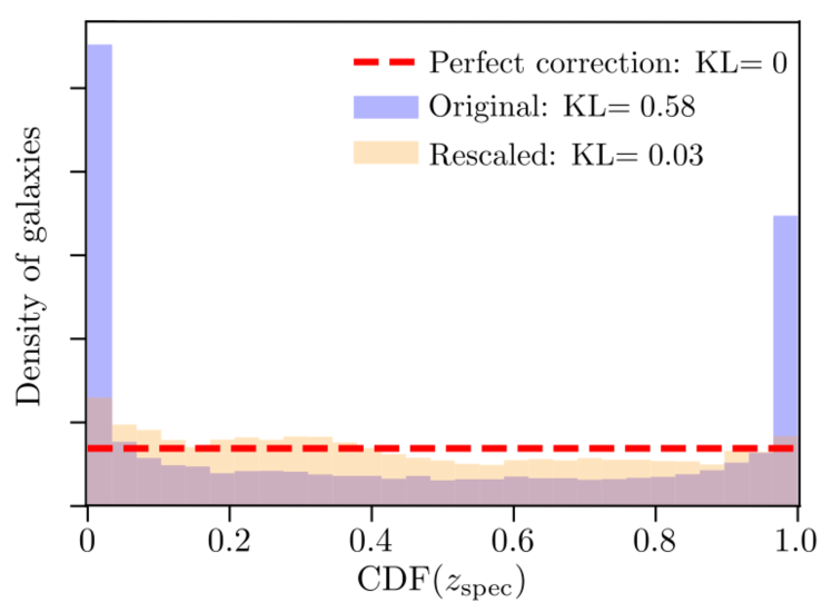
For each galaxy in COSMOS2015 having a spectroscopic redshift and matching a DES detection, is integrated to a cumulative distribution function (CDF) The value for a distribution of objects is the Probability Integral Transform (PIT) (Dawid, 1984; Angus, 1994). If is a true, statistically rigorous PDF of the spectroscopic redshifts, the PIT values should be uniformly distributed between 0 and 1. In Figure 1 we show in blue the distribution of PIT values for the original ’s. The peaks at 0 and at 1 indicate that the widths of the are underestimated and need to be broadened, and the asymmetry means that a small global offset should be applied to them.
We recalibrate the ’s by positing that the true PDF can be well approximated by applying the following transformation to the original :
| (2) |
In the first term, is slightly broadened and shifted by convolution with a Gaussian of width and center . The second term adds in a Cauchy distribution about the median value of the original to allow for long tails. The free parameters are found using the Nelder-Mead method of scipy.stats.minimise to minimize the Kullback-Leibler (KL) divergence between the histogram of CRPS values and the expected uniform distribution. The best-fitting recalibration parameters are derived using a randomly selected 50% of the spectroscopic catalog and then validated on the remaining 50%. The histogram of CRPS of the validation samples after recalibration is shown in Figure 1 by the orange histograms.
Going into further detail: we determine the best-fitting remapping parameters independently for six subsets in bins of -band MAG_AUTO (Bertin & Arnouts, 1996) magnitude bounded by [16.1, 20.72, 21.48, 21.98, 22.40, 23.03, 99]. The bins are chosen so that they are each populated by approximately 4000 spectra. Remapping in bins of magnitude is seen to yield lower KL values than remapping in redshift bins, or with no binning. We find that the KL values of the training data and the validation data are very similar, indicating that we are not over-fitting. The KL divergences in the first and last bin decrease from and , respectively, with even greater improvement for the full sample as noted in Figure 1. The only parameter relevant for the mean redshift calibration performed in § 4 is the shift in the mean of the , . The sizes of these in each magnitude bin are all , much smaller than the uncertainty of our ensemble mean redshifts.
2.3 Simulated sky catalogs
We also draw upon simulated data sets generated specifically for the DES collaboration. Specifically, we make use of the Buzzard-v1.1 simulation, a mock DES Y1 survey created from a set of dark-matter-only simulations. This simulation and the galaxy catalog construction are described in detail elsewhere (DeRose et al., 2017; Wechsler et al., 2017; MacCrann et al., 2017), so here we provide only a brief overview. Buzzard-v1.1 is constructed from a set of 3 -body simulations run using L-GADGET2, a version of GADGET2 modified for memory efficiency, with box lengths ranging from 1–4 Gpc from which light-cones were constructed on the fly.
Galaxies are added to the simulations using the Adding Density Dependent GAlaxies to Light-cone Simulations algorithm [ADDGALS, Wechsler et al. 2017]. Spectral energy distributions (SEDs) are assigned to the galaxies from a training set of spectroscopic data from SDSS DR7 (Cooper et al., 2011) based on local environmental density. These SEDs are integrated in the DES pass bands to generate magnitudes. Galaxy sizes and ellipticities are drawn from distributions fit to SuprimeCam -band data (Miyazaki et al., 2002). The galaxy positions, shapes and magnitudes are then lensed using the the multiple-plane ray-tracing code, Curved-sky grAvitational Lensing for Cosmological Light conE simulatioNS [CALCLENS, Becker (2013)]. The simulation is cut to the DES Y1 footprint, and photometric errors are applied to the lensed magnitudes by copying the noise map of the FLUX_AUTO measurements in the real catalog. More explicitly, the error on the observed flux is determined only by the limiting magnitude at the position of the galaxy, the exposure time, and the noise-free apparent magnitude of the galaxy itself.
2.3.1 Science sample selection in simulations
The source-galaxy samples in simulations are selected so as to roughly mimic the selections and the redshift distributions of the metacalibration shear catalog described in Zuntz et al. (2017). This is done by first applying flux and size cuts to the simulated galaxies so as to mimic the thresholds used in the Y1 data by using the Y1 depth and PSF maps. The weak lensing effective number density in the simulation is matched to a preliminary version of the shape catalogs, and is about 7 per cent higher than for the final, unblinded metacalibration catalog. Truth values for redshift, flux and shear are of course available as well as the simulated measurements.
COSMOS-like catalogs are also generated from the Buzzard simulated galaxy catalogs by cutting out 367 non-overlapping COSMOS-shaped footprints from the simulation.
3 Photometric redshift estimation
In this section we describe the process of obtaining photometric redshifts for DES galaxies. We note that we only use the DES bands in this process. We have found that the band adds little to no predictive power.
3.1 Bayesian Photometric Redshifts (BPZ)
Posterior probabilities were calculated for each source galaxy using BPZ∗, which is a variant of the Bayesian algorithm described by Benítez (2000), and has been modified to provide the photometric redshift point predictions and PDFs required by the DES collaboration directly from fits-format input fluxes, without intermediate steps. The BPZ∗ code is a distilled version of the distributed BPZ code, and in particular assumes the synthetic template files for each filter have already been generated. Henceforth we will refer to these simply as “BPZ” results.
3.1.1 Per-galaxy posterior estimation
The redshift posterior is calculated by marginalising over a set of interpolated model spectral templates, where the likelihood of a galaxy’s photometry belonging to a given template at a given redshift is computed via the between the observed photometry and those of the filter passbands integrated over the model template. The model templates are grouped into three classes, nominally to represent elliptical, spiral and star-burst galaxies. These classes, it is assumed, follow distinct redshift-evolving luminosity functions which can be used to create a magnitude-dependent prior on the redshift posterior of each object, a.k.a. the “luminosity prior”. The prior comprises two components, a spectral class prior which is dependent only on observed magnitude, and the redshift prior of each class—which is itself also magnitude dependent (see Benítez 2000 for more detail).
Six base template spectra for BPZ are generated based on original models by Coleman, Wu & Weedman (1980) and Kinney et al. (1996). The stellar locus regression used for the DES Y1 data ensures uniformity of color across the footprint, but there may be small differences in calibration with respect to the empirical templates we wish to use. Moreover, these original templates are derived from galaxies at redshift zero, while our source galaxies cover a wide range in redshift, with an appreciable tail as high as . The colors of galaxies evolve significantly over this redshift range, even at fixed spectral type. Failure to account for this evolution can easily introduce biases in the redshift posteriors that subsequently require large model bias corrections (see Bonnett et al. 2016, for instance). To address these two issues, we compute evolution/calibration corrections to the template fluxes.
We match low-resolution spectroscopic redshifts from the PRIMUS DR1 dataset (Coil et al., 2011; Cool et al., 2013) to high signal-to-noise DES photometry and obtain the best fit of the six basic templates to each of the highest quality PRIMUS objects (quality = 4) at their spectroscopic redshift. The flux of each template in each filter is then corrected as a function of redshift by the median offset between the DES photometry and the template prediction, in a sliding redshift window of width . The calibration sample numbers 72,176 galaxies and reaches the full depth of our science sample () while maintaining a low rate of mis-assigned redshifts.333The outlier fraction of quoted in Cool et al. (2013) includes all objects that lie more than from their true redshift. The difference in template photometry caused by such a small change in redshift is well within the scatter of our computed DES - template offsets. Of greater concern is the fraction of objects with large redshift differences, which is . Although the incompleteness in PRIMUS is broadly independent of galaxy color (Cool et al., 2013) and each template is calibrated separately, we nevertheless expect small residual inaccuracies in our calibration to remain. Our COSMOS and WZ validation strategies serve to calibrate such errors in BPZ assignments.
A complete galaxy sample is required for deriving the luminosity prior we use with BPZ. No spectroscopic samples are complete to the limit of our source galaxy sample, and so we turn to the accurate photometric redshift sample in the COSMOS field from Laigle et al. (2016), which is complete to the depth of our main survey area despite being selected in the -band. The prior takes the form of smooth exponential functions (see Benítez 2000), which we fit to the COSMOS galaxy population by determining galaxy types at their photometric redshift. Because BPZ uses smooth functions rather than the population directly, the luminosity prior used for obtaining posterior redshift probabilities does not replicate the high-frequency line-of-sight structure in the COSMOS field.
BPZ is run on the MOF fluxes (see §2) to determine for metacalibration and im3shape, while for the five metacalibration catalogs—the real one and the four artificially sheared versions—BPZ is run on the metacalibration fluxes to determine bin assignments (cf. §3.3 for details). The luminosity prior is constructed from MOF -band fluxes for both catalogues. For the Buzzard simulated galaxy catalogs, BPZ is run on the single mock flux measurement produced in the simulation.
We also explored a further post-processing step as in §2.2.3, but applied to the DES BPZ photo-z PDFs. We used the spectroscopic training data, which is not used in BPZ, to recalibrate the PDFs in bins of -band magnitude. We find that this rescaling did not noticeably change the mean or widths of the PDFs on average, and that the statistical properties of the redshift distributions in each tomographic bin also remain unchanged.
3.1.2 Known errors
During BPZ processing of the Y1 data, three configuration and software errors were made.
First, the metacalibration catalogs were processed using MOF -band magnitudes for evaluating the BPZ prior rather than Metacal fluxes. This is internally consistent for BPZ, but the use of flux measurements that do not exist for artificially sheared galaxies means that the metacalibration shear estimates are not properly corrected for selection biases resulting from redshift bin assignment. We note that small perturbations to the flux used for assigning the luminosity prior have very little impact on the resulting mean redshift and the colors used by BPZ in this run are correctly measured by metacalibration on unsheared and sheared galaxy images. Rerunning BPZ with the correct, Metacal inputs for -band magnitude on a subset of galaxies indicates that the induced multiplicative shear bias is below in all redshift bins, well below both the level of statistical errors in DES Y1 and our uncertainty in shear bias calibration. We therefore decide to tolerate the resulting systematic uncertainty.
Second, the SLR adjustments to photometric zeropoints were not applied to the observed Metacal fluxes in the Y1 catalogs before input to BPZ. The principal result of this error is that the observed magnitudes are no longer corrected for Galactic extinction. This results in a shift in the average of the source population of each bin, and a spatially coherent modulation of the bin occupations and redshift distributions across the survey footprint. In §4 we describe a process whereby the mean can be accurately estimated by mimicking the SLR errors on the COSMOS field. In Appendix B we show that the spurious spatial variation of the redshift distributions causes negligible errors in our estimation of the shear two-point functions used for cosmological inference, and zero error in the galaxy-galaxy lensing estimates.
Finally, when rewriting BPZ for a faster version, BPZ∗, two bugs were introduced in the prior implementation, one causing a bias for bright galaxies ( band magnitude ) and another which forced uniform prior abundance for the three galaxy templates. These bugs were discovered too late in the DES Y1 analysis to fix. They cause differences in that are subdominant to our calibration uncertainties (below 0.006 among all individual bins). In addition, they are fully calibrated by both COSMOS (which uses the same implementation) and WZ, and hence do not affect our cosmological analysis. We have since implemented all of the above bug fixes, and applied the SLR adjustments correctly, and find negligible changes in the shape and mean of the BPZ PDFs, which are fully within the combined systematic uncertainties.
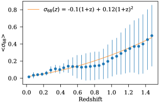
3.1.3 Per-galaxy photo- precision
While are the critical inputs to cosmological inference, it is sometimes of use to know the typical size of the redshift uncertainty for individual galaxies. We define for each as the half-width of the 68 percentile region around the median. We select 200,000 galaxies from the metacalibration catalog at random, and determine the average in bins of redshift according to the median of . We find that this mean is well fit by a quadratic polynomial in mean BPZ redshift and present the best-fitting parameters in Figure 2.
Further metrics of the performance of individual galaxies’ photo-’s but with respect to truth redshifts are provided in §4.7.
3.2 Directional Neighborhood Fitting (DNF)
Directional Neighborhood Fitting (DNF) (De Vicente, Sanchez & Sevilla-Noarbe, 2016) is a machine-learning algorithm for galaxy photometric redshift estimation. We have applied it to reconstruct the redshift distributions for the metacalibration catalogs. DNF takes as reference a training sample whose spectroscopic redshifts are known. Based on the training sample, DNF constructs the prediction hyperplane that best fits the neighborhood of each target galaxy in multiband flux space. It then uses this hyperplane to predict the redshift of the target galaxy. The key feature of DNF is the definition of a new neighborhood, the Directional Neighborhood. Under this definition — and leaving apart degeneracies corresponding to different galaxy types — two galaxies are neighbors not only when they are close in the Euclidean multiband flux space, but also when they have similar relative flux in different bands, i.e. colors. In this way, the neighborhood does not extend in multiband flux hyperspheres but in elongated hypervolumes that better represent similar color, and presumably similar redshift. As described in §3.3, these DNF photo- predictions are used to classify the galaxies in tomographic redshift bins.
A random sample from the of an object is approximated in the DNF method by the redshift of the nearest neighbor within the training sample. It is used as the sample for reconstruction and interpreted in section §3.3 as a random draw from the underlying per-galaxy posterior.
The training sample used for Y1 DNF prediction was collected by the DES Science Portal team (Gschwend et al., 2017) from different spectroscopic surveys and includes the VIPERS 2nd data release (Scodeggio et al., 2016). The validation of the predictions was based on COSMOS2015 photo-’s. Objects near the COSMOS data were removed from the training sample. Since the machine learning algorithm can correct for imperfections in the input photometry giving a representative training set, both training and photo- predictions are based on Metacal photometry without SLR- adjustments, for all runs on DNF.
The fiducial DES Y1 cosmological parameter estimation uses the BPZ photo-’s, and DES Collaboration et al. (2017) demonstrate that these estimates are robust to substitution of DNF for BPZ.
The distributions of BPZ and DNF are not expected to be identical, because the algorithms may make different bin assignments for the same source. We therefore do not offer a direct comparison. We do, however, repeat for DNF all of the validation processes described herein for the BPZ estimates. The results for DNF are given in Appendix C.
3.3 Binning and initial estimation
| shear catalog | step | BPZ | DNF |
|---|---|---|---|
| binned by: | Metacal | Metacal | |
| metacalibration | by stacking: | MOF | Metacal |
| calibration by: | COSMOS + WZ | COSMOS + WZ | |
| binned by: | MOF | — | |
| im3shape | by stacking: | MOF | — |
| calibration by: | COSMOS + WZ | — |
Both photo- codes yield 6 different posterior distributions for each galaxy in the Y1 shape catalogs, conditional on either the MOF, the unsheared Metacal, or the four sheared Metacal flux measurements. In this section, we describe how these are used to define source redshift bins and provide an initial estimate of the lensing-weighted of each of these bins. Table 1 gives an overview of these steps.
Galaxies are assigned to bins based on the expectation value of their posterior, . We use four bins between the limits . These tomographic boundaries exclude and that have large photo- biases. We place three tomographic bins at with approximately equal effective source density , a proxy for the statistical uncertainty of shear signals in the metacalibration catalog, since is the upper limit of the WZ constraints. The fourth bin, is thus validated only by the COSMOS method.
For metacalibration sources, this bin assignment is made based on the of the photo- run on Metacal photometry, instead of MOF photometry. The reason for this is that flux measurements, and therefore photo- bin assignments, can depend on the shear a galaxy is subject to. This can cause selection biases in shear due to photo- binning, which can be corrected in metacalibration. The latter requires that the bin assignment can be repeated using a photo- estimate made from measurements made on artificially sheared images of the respective galaxy (cf. Huff & Mandelbaum, 2017; Sheldon & Huff, 2017; Zuntz et al., 2017), and only the Metacal measurement provides that.
For im3shape sources, the bin assignment is made based on the of the photo- run on MOF photometry, which has higher and lower susceptibility to blending effects than Metacal photometry. This provides more precise (and possibly more accurate) photo- estimates.
We note that this means that for each combination of shear and photo- pipeline, bin assignments and effective weights of galaxies are different. The redshift distributions and calibrations derived below can therefore not be directly compared between the different variants.
The stacked redshift distribution of each of the tomographic bins is estimated by the lensing-weighted stack of random samples from the of each of all galaxies in bin . Given the millions of galaxies in each bin, the noise due to using only one random sample from each galaxy is negligible. For both the metacalibration and im3shape catalogs, we use random samples from the estimated by BPZ run on MOF photometry to construct the , this being the lower-noise and more reliable flux estimate. In the case of DNF, we use the Metacal photometry run for both the binning and initial estimation.
By the term lensing-weighted above, we mean the effective weight a source has in the lensing signals we measure in Troxel et al. (2017) and Prat et al. (2017). In the case of metacalibration, sources are not explicitly weighted in these papers. Since the ellipticities of galaxies in metacalibration have different responses to shear (Huff & Mandelbaum, 2017; Sheldon & Huff, 2017), and since we measure correlation functions of metacalibration ellipticities that we then correct for the mean response of the ensemble, however, sources do have an effective weight that is proportional to their response. As can be derived by considering a mixture of subsamples at different redshifts and with different mean response, the correct redshift distribution to use is therefore one weighted by where the ’s are shear responses defined in Zuntz et al. (2017). In the case of im3shape, explicit weights are used in the measurements, and sources have a response to shear with the calibrated multiplicative shear bias (Zuntz et al., 2017). The correct effective weights for im3shape are therefore .
We note that for other uses of the shape catalogs, such as with the optimal estimator (Sheldon et al., 2004), the effective weights of sources could be different, which has to be accounted for in the photo- calibration.
4 Validating the redshift distribution using COSMOS multi-band photometry
In Bonnett et al. (2016) we made use of COSMOS photometric redshifts as an independent estimate and validation of the redshift distribution of the weak lensing source galaxies. We made cuts in magnitude, FWHM and surface brightness to the source catalogue from DECam images in the COSMOS field that were depth-matched to the main survey area. These cuts approximated the selection function of the shape catalogues used for the cosmic shear analysis. Similar techniques that find COSMOS samples of galaxies matched to a lensing source catalog by a combination of magnitude, color and morphological properties have been applied by numerous studies (Applegate et al., 2014; Hoekstra et al., 2015; Okabe & Smith, 2016; Cibirka et al., 2017; Amon et al., 2017). In the present work, we modify the approach to reduce statistical and systematic uncertainty on its estimate of mean redshift and carefully estimate the most significant sources of systematic error.
We wish to validate the derived for a target sample A of galaxies using a sample B with known redshifts. Ideally, for every galaxy in A, we would find a galaxy in B that looks exactly like it when observed in the same conditions. The match would need to be made in all properties we use to select and weight the galaxy in the weak lensing sample that also correlate with redshift.
Then the mean redshift distribution of the matched B galaxies, weighted the same way as the A galaxies are for WL measures, will yield the desired . This goal is unattainable without major observational, image processing and simulation efforts, but we can approximate it with a method related to the one of Lima et al. (2008) and estimate the remaining uncertainties. We also need to quantify uncertainties resulting from the finite size of sample B, and from possible errors in the “known” redshifts of B. Here our sample A are the galaxies in either the im3shape or metacalibration Y1 WL catalogs, spread over the footprint of DES Y1, and sample B is the COSMOS2015 catalog of Laigle et al. (2016).
4.1 Methodology
We begin by selecting a random subsample of 200,000 galaxies from each WL source catalog, spread over the whole Y1 footprint, and assigning to each a match in the COSMOS2015 catalog. The match is made by MOF flux and pre-seeing size (not by position), and the matching algorithm proceeds as follows, for each galaxy in the WL source sample:
-
1.
Gaussian noise is added to the DES MOF fluxes and sizes of the COSMOS galaxies until their noise level is equal to that of the target galaxy. COSMOS galaxies whose flux noise is above that of the target galaxy are considered ineligible for matching. While this removes 13% of potential DES-COSMOS pairs, this is unlikely to induce redshift biases, because the noise level of the COSMOS catalog is well below that of the Y1 survey in most regions of either, so it should be rare for the true COSMOS “twin” of a Y1 source to have higher errors. The discarded pairs predominantly are cases of large COSMOS and small Y1 galaxies (since large size raises flux errors), and the size mismatch means these galaxies would never be good matches. Other discarded pairs come from COSMOS galaxies lying in a shallow region of the DECam COSMOS footprint, such as near a mask or a shallow part of the dither pattern, and this geometric effect will not induce a redshift bias. Note that the MOF fluxes used here make use of the SLR zeropoints, for both COSMOS and Y1 catalogs. The size metric is the one produced by metacalibration.
-
2.
The matched COSMOS2015 galaxy is selected as the one that minimizes the flux-and-size
(3) where and are the fluxes in band and the size, respectively, and and are the measurement errors in these for the chosen source. We also find the galaxy that minimizes the from flux differences only:
(4) If the least is smaller than of the galaxy with the least flux-and-size , we use this former galaxy instead. Without this criterion, we could be using poor matches in flux (which is more predictive of redshift than size) by requiring a good size match (that does not affect redshift distributions much). It applies to about 15 per cent of cases.
-
3.
A redshift is assigned by drawing from the of the matched COSMOS2015 galaxy, using the rescaling of §2.2.3.
-
4.
A bin assignment is made by running the BPZ procedures of §3.1 on the noise-matched fluxes of the COSMOS match, using the mean value of each galaxy’s posterior , as before. For the im3shape catalog, the MOF photometry of the COSMOS galaxy is used, just as is done for the Y1 main survey galaxies. The metacalibration treatment is more complex: we generate simulated Metacal fluxes for the COSMOS galaxy via
(5) This has the effect of imposing on COSMOS magnitudes the same difference between Metacal and MOF as is present in Y1, thus imprinting onto COSMOS simulations any errors in the Y1 catalog metacalibration magnitudes due to neglect of the SLR or other photometric errors. For the flux uncertainty of these matched fluxes, for both MOF and Metacal, we assign the flux errors of the respective Y1 galaxy.
-
5.
The effective weak lensing weight of the original source galaxy is assigned to its COSMOS match (cf. §3.3).
As a check on the matching process, we examined the distribution of the between matched galaxies. The distribution is skewed toward significantly lower values than expected from a true distribution with 4 degrees of freedom. This indicates that the COSMOS-Y1 matches are good: COSMOS galaxies are photometrically even more similar to the Y1 target galaxies than they would be to re-observed versions of themselves.
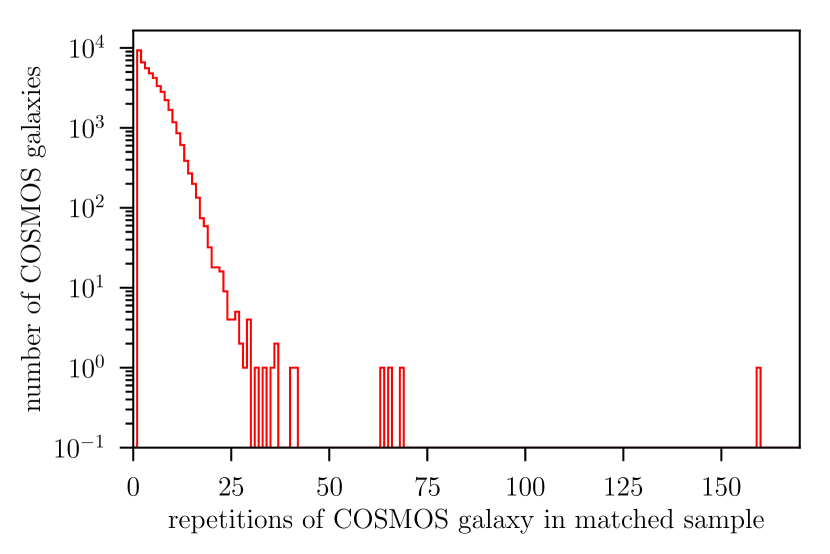
A second check on the matching algorithm is to ask whether the individual COSMOS galaxies are being resampled at the expected rates. As expected, most sufficiently bright galaxies in COSMOS are used more than once, while the faintest galaxies are used more rarely or never. Figure 3 shows the number of times each of the COSMOS galaxies is matched to metacalibration (if it is bright enough to be matched at all) in our fiducial matched catalog. We see that there is no unwanted tendency for a small fraction of the COSMOS galaxies to bear most of the resampling weight. All COSMOS galaxies with more than 50 repetitions are brighter than and have a typical redshift of .
We now use the matched COSMOS galaxy set to produce an estimate of the difference in mean redshift between the -predicted distribution and the “truth” provided by COSMOS2015 for all galaxies assigned to a given source bin:
| (6) |
where the sums run over all matched COSMOS2015 galaxies and all galaxies in the original source sample .
This construction properly averages over the observing conditions (including photometric zeropoint errors) and weights of the Y1 WL sources. These estimated values using BPZ are tabulated in Table 2 for both WL source catalogs.
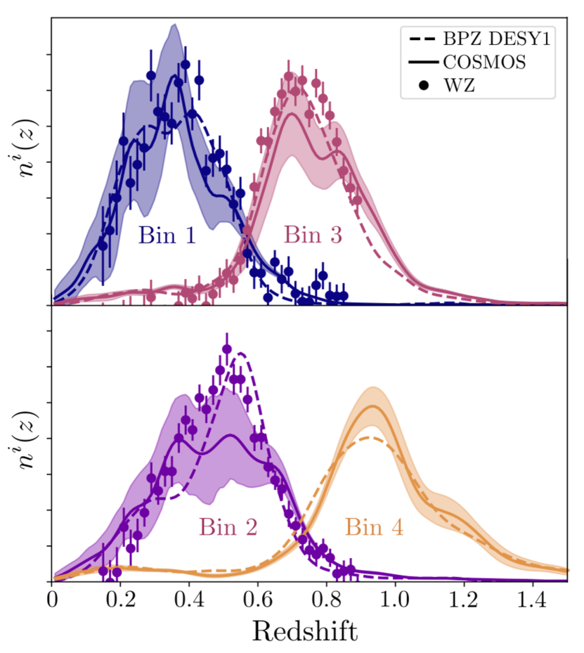
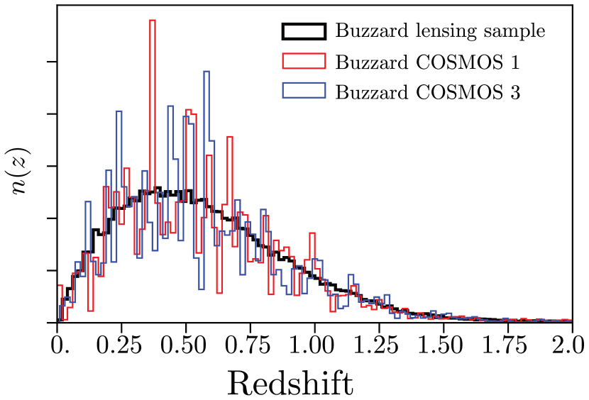
The COSMOS validation also yields an estimate of by a weighted average of the rescaled ’s of the matches (or, equivalently, of samples drawn from them). Figure 4 plots these resampled-COSMOS estimates along with the original from BPZ. Here it is apparent that in some bins, these two estimates differ by more than just a simple shift in redshift—the shapes of the distributions differ significantly. In §6.2 we demonstrate that these differences do not bias our cosmological inferences.
| Value | Bin 1 | Bin 2 | Bin 3 | Bin 4 |
|---|---|---|---|---|
| range | 0.20–0.43 | 0.43–0.63 | 0.63–0.90 | 0.90-1.30 |
| COSMOS footprint sampling | ||||
| COSMOS limited sample size | ||||
| COSMOS photometric calibration errors | ||||
| COSMOS hidden variables | ||||
| COSMOS errors in matching | ||||
| COSMOS single-bin uncertainty | ||||
| metacalibration | ||||
| COSMOS final , tomographic uncertainty | ||||
| WZ final | — | |||
| Combined final | ||||
| im3shape | ||||
| COSMOS final , tomographic uncertainty | ||||
| WZ final | — | |||
| Combined final | ||||
In the following subsections, we determine several contributions to the uncertainty of these . All of these are presented for the metacalibration sample binned by BPZ redshift estimates. For im3shape galaxies with BPZ, we use the same uncertainties. Results for DNF are in Appendix C.
From the resampling procedure, we also determine common metrics on the photo- performance in § 4.7.
4.2 Sample variance contribution
The first contribution to the uncertainty in the COSMOS ’s is from sample variance from the small angular size of the COSMOS2015 catalog. Any attempt at analytic estimation of this uncertainty would be complicated by the reweighting/sampling procedure that alters the native of the COSMOS line of sight, so we instead estimate the covariance matrix of the by repeating our procedures on different realizations of the COSMOS field in the Buzzard simulated galaxy catalogs.
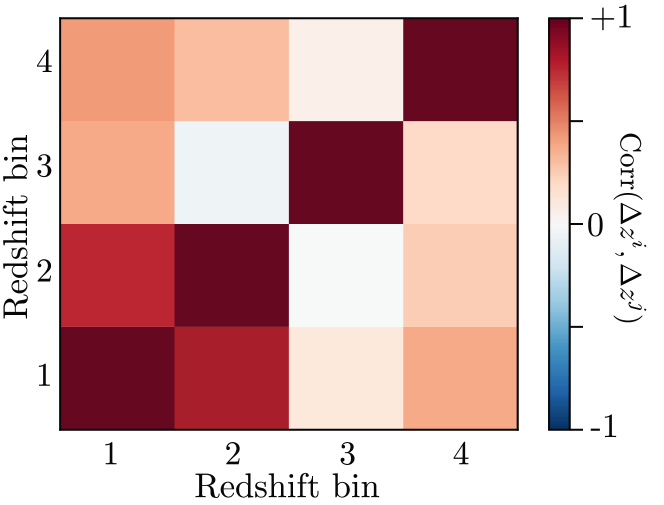
The resampling procedure of §4.1 is repeated using a fixed single draw of 200,000 galaxies from a Buzzard simulated Y1 WL sample (§2.3) as catalog A, and 367 randomly placed COSMOS-shaped cutouts from the Buzzard truth catalog, i.e. a catalog with noiseless flux information, as catalog B. Each of these yields an independent of the matched COSMOS catalogs (cf. Figure 5), and consequently an independent sample variance realization of the . There are significant correlations between the bins, especially bins 1 and 2, as shown in §6. The diagonal elements are listed as “COSMOS footprint sampling” in Table 2.
Since we use the same subset of the Buzzard lensing sample for each of the COSMOS-like resamplings, this variance estimate does not include the uncertainty due to the limited subsample size of 200,000 galaxies. We estimate the latter effect by resampling of the in this sample, and find it to be subdominant ( in all redshift bins, “limited sample size” in Table 2).
4.3 Photometric calibration uncertainty
The DECam photometry of the COSMOS field has uncertainties in its zeropoint due to errors in the SLR-based calibration. While the Y1 catalog averages over the SLR errors of many fields, the validation is sensitive to the single realization of SLR errors in the COSMOS field. We estimate the distribution of zeropoint errors by comparing the SLR zeropoints in the Y1 catalog to those derived from the superior “forward global calibration module” (FGCM) and reddening correction applied to three years’ worth of DES exposures by Burke et al. (2017). In this we only use regions with Galactic extinction , since the COSMOS field has relatively low extinction and strong reddening might cause larger differences between the FGCM and SLR calibration. The root-mean-square zeropoint offsets between SLR and FGCM calibration are between 0.007 () and 0.017 ().
We estimate the impact on by drawing 200 mean-subtracted samples of photometric offsets from the observed (FGCM-SLR) distribution, applying each to the COSMOS fluxes, and repeating the derivation of as per §4.1. Table 2 lists the uncertainty of the of each of the four tomographic bins due to those, which are .
4.4 Hidden-variable uncertainty
We have matched COSMOS galaxies to the shear catalog galaxies by their fluxes and by their estimated pre-seeing size. This set of parameters is likely not completely predictive of a galaxy’s selection and weight in our shear catalog. Other morphological properties (such as the steepness of its profile) probably matter and do correlate with redshift (e.g. Soo et al., 2017). In addition, the matching in size is only done in 85 per cent of cases to begin with § 4.1.
To estimate the effect of any variables hidden to our matching algorithm, we repeat the process while ignoring the size variable. We find changes in for metacalibration to be in the four bins. Soo et al. (2017) found that the single morphological parameter that provides the greatest improvement in and outlier fraction is galaxy size. Since we therefore expect the size to have the strongest influence on both lensing and redshift, and we are correcting for size, we estimate the potential influence of any further variables as no more than half of the size effect. We do not assume that these systematic errors found in simulations are exactly equal in the data - rather, we only assume that the two are of similar size, and thus use the rms of offsets found in the simulation as the width of a Gaussian systematic uncertainty on the data. We take half of the quadratic mean of the shifts in the four redshift bins, as our estimate of the hidden-variable uncertainty in each bin. These biases are likely to be correlated between bins. In §4.6 we describe a modification to our single-bin uncertainties that accounts for potential correlations.
4.5 Systematic errors in matching
Even in the absence of the above uncertainties, the resampling algorithm described above might not quite reproduce the true redshift distribution of the input sample. The matching algorithm may not, for example, pick a COSMOS galaxy which is an unbiased estimator of the target galaxy’s redshift, especially given the sparsity and inhomogeneous distribution of the COSMOS sample in the four- to five-dimensional space of fluxes and size.
We estimate the size of this effect on using the mean offset in binned mean true redshift of the 367 realizations of resampled COSMOS-like catalogs in the Buzzard simulations (see § 4.2) from the binned mean true redshift of the underlying Buzzard shape sample.
We find differences in mean true redshift of sample A - matched B of (0.0027, 0.0101, 0.0094, 0.004) for the four redshift bins. Since the simulation is not fully realistic, we do not attempt to correct the result of our resampling with these values. Rather, we take them as indicators of possible systematic uncertainties of the resampling algorithm. Following the argument in section §4.4 ,we thus use the quadratic mean of these values (0.0073) as a systematic uncertainty in each bin.
4.6 Combined uncertainties and correlation between redshift bins
The final uncertainties on the are estimated by adding in quadrature the contributions listed above, yielding the “COSMOS total uncertainty” in Table 2. These values are derived independently for each redshift bin, but it is certain that the have correlated errors, e.g. from sample variance as shown in Figure 6, and such correlations should certainly be included in the inference of cosmological parameters. The values of the off-diagonal elements of the combined COSMOS covariance matrix, are, however, difficult to estimate with any precision. In Appendix A we demonstrate that by increasing the diagonal elements of the covariance matrix by a factor and nulling the off-diagonal elements, we can ensure that any inferences based on the are conservatively estimated for any reasonable values of the off-diagonal elements. We therefore apply a factor of 1.6 to all of the single-bin uncertainties in deriving the “COSMOS final ” constraints for metacalibration and im3shape given in Table 2.
4.7 Standard photo-z performance metrics
| metric | ||||
|---|---|---|---|---|
| BPZ metacalibration binning, MOF | ||||
| Outlier Fraction % | ||||
| DNF metacalibration | ||||
| Outlier Fraction % | ||||
Although not a critical input to the cosmological tests of DES Collaboration et al. (2017), we determine here some standard metrics of photo- performance. We define the residual as the difference between the mean of the using the MOF photometry and a random draw from the COSMOS matched during resampling. We use a random draw from rather than the peak, so that uncertainty in these “truth” ’s is included in the metrics. Because the width of is much smaller than that of , this does not affect the results significantly.
We define as the 68% spread of around its median. In this section measures the departure of the mean of from the true , whereas the in Figure 2 is a measure of width of independent of any truth redshifts. We also measure the outlier fraction, defined as the fraction of data for which . If the redshift distribution were Gaussian, the outlier fraction would be 5%, and this metric is a measure of the tails of the distribution.
We calculate the uncertainties on these metrics from sample variance, COSMOS photometric calibration uncertainty, and selection of the lensing sample by hidden variables (cf. § 4.2-4.4). We add each of the these uncertainties in quadrature in each tomographic bin, and highlight that the largest source of uncertainty is due to sample variance.
Table 3 presents the metric values and uncertainties of the galaxies in each redshift bin, using the metacalibration sample and binning.
5 Combined constraints
To supplement the constraints on derived above using the COSMOS2015 photo-’s, we turn to the “correlation redshift” methodology (Newman, 2008; Ménard et al., 2013; Schmidt et al., 2013) whereby one measures the angular correlations between the unknown sample (the WL sources) and a population of objects with relatively well-determined redshifts. In our case the known population are the redMaGiC galaxies, selected precisely so that their colors yield high-accuracy photometric redshift estimates.
An important complication of applying WZ to DES Y1 is that we do not have a sufficient sample of galaxies with known redshift available that spans the redshift range of the DES Y1 lensing source galaxies – the redMaGiC galaxies do not extend beyond . Constraints on the mean redshift of a source population can still be derived in this case, but only by assuming a shape for the distribution, whose mean is then determined by the clustering signal in a limited redshift interval. A mismatch in shape between the assumed and true is a source of systematic uncertainty in such a WZ analysis. One of the main results of Gatti et al. 2017, which describes the implementation and full estimation of uncertainties of the WZ method for DES Y1 source galaxies, is that while this systematic uncertainty needs to be accounted for, it is not prohibitively large. This statement is validated in Gatti et al. 2017 for the degree of mismatch between the true and the found in a number of photometric redshift methods applied to simulated galaxy catalogs. The redshift distributions of the DES weak lensing sources as estimated by BPZ, as far as we can judge this from the comparison with the COSMOS estimates of their true , show a similar level of mismatch to the truth. The systematic uncertainty budget derived in Gatti et al. (2017) is therefore applicable to the data. We do not, however, attempt to correct the systematic offsets in WZ estimates of introduced due to this effect – for this, we would require the galaxy populations and photometric measurements in the simulations to be perfectly realistic.
The method is applied to DES Y1 data in Davis et al. (2017a). A similar analysis was performed on the DES SV data set in Davis et al. (2017b). The resultant estimates of are listed in Table 2 and plotted in Figure 7. The full ’s estimated from the WZ method are plotted in Figure 4. Note that the WZ method obtains no useful constraint for bin 4 because the redMaGiC sample is confined to and thus has little overlap with bin 4. Due to the lack of independent confirmation, the redshift calibration of this bin should be used with greater caution – in DES Collaboration et al. (2017) and Gruen et al. (2017), we indeed show that constraints do not significantly shift when the bin is removed from the analysis.
In the three lower redshift bins, the COSMOS and WZ validation methods generate estimates of that are fully consistent. Indeed even their curves show qualitative agreement. We therefore proceed to combine their constraints on to yield our most accurate and reliable estimates. The statistical errors of the COSMOS and WZ methods are uncorrelated (sample variance in the COSMOS field vs. shot noise in the measurements of angular correlations in the wide field). The dominant systematic errors of the two methods should also be uncorrelated, e.g. shortcomings in our resampling for COSMOS vs. uncertainties in the bias evolution of source galaxies for WZ. We are therefore confident that we can treat the COSMOS and WZ constraints as independent, and we proceed to combine them by multiplying their respective 1-dimensional Gaussian distributions for each i.e. inverse-variance weighting. In bin 4, the final constraints are simply the COSMOS constraints since WZ offers no information.
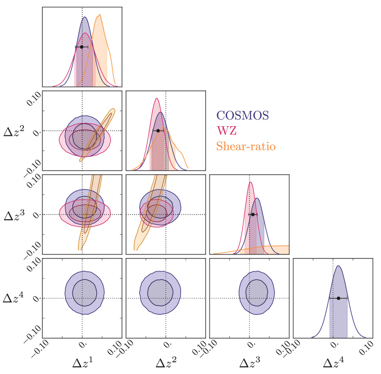
The resultant constraints, listed for both metacalibration and im3shape catalogs in Table 2, are the principal result of this work, and are adopted as input to the cosmological inferences of Troxel et al. (2017) and DES Collaboration et al. (2017). The adopted 68%-confidence ranges for each are denoted by the gray bands in the 1-d marginal plots of Figure 7.
One relevant question is whether our calibration finds that significant non-zero shifts are required to correct the photo- estimates of the mean redshift. For the fiducial metacalibration BPZ, this is not the case: the is 3.5 with 4 bins. However, the combined is non-zero at for im3shape BPZ and the is non-zero at for metacalibration DNF, indicating that there are significant alterations being made to some of the estimates.
A further check of the accuracy of our estimation is presented by Prat et al. (2017) using the ratios of lensing shear on the different source bins induced by a common set of lens galaxies. Initially proposed as a cosmological test (Jain & Taylor, 2003), the shear ratio is in fact much less sensitive to cosmological parameters than to potential errors in either the calibration of the shear measurement or the determination of the We plot in Figure 7 the constraints on inferred by Prat et al. (2017) after marginalization over the estimated errors in shear calibration and assuming a fixed CDM cosmology with . The shear-ratio test is fully consistent with the COSMOS and WZ estimates of though we should keep in mind that this test is also dependent on the validity of the shear calibration and some other assumptions in the analysis, and importantly is covariant with the WZ method, because both methods rely on correlation functions as measured with respect to the same galaxy samples..
6 Use for cosmological inference
The final rows of Table 2 provide the prior on errors in the redshift distributions used during inference of cosmological parameters for the DES Y1 data, under the assumption that errors in the resulting from the photo- analysis follow Equation (1). Determination of redshift distributions is and will continue to be one of the most difficult tasks for obtaining precision cosmology from broadband imaging surveys such as DES, so it is important to examine the potential impact of assumptions in our analysis choices. Further, we wish to identify areas where our methodology can be improved and thereby increase the precision and accuracy of future cosmological analyses.
6.1 Dependence on COSMOS2015 redshifts
First, we base our COSMOS validation on the COSMOS2015 redshift catalog derived from fitting spectral templates to 30-band fluxes. Our COSMOS validation rests on the assumption that Laigle et al. (2016) have correctly estimated the redshift posteriors of their sources. Overall, redshift biases in the COSMOS2015 redshifts are significant, unrecognized sources of error in our cosmological inferences if they approach or exceed the –0.02 range of uncertainty in our constraints. More precisely, this bias must accrue to the portion of the COSMOS2015 catalog that is bright enough to enter the DES Y1 shear catalogs.
For the subset of their sources with spectroscopic redshifts, Laigle et al. (2016) report that galaxies in the magnitude interval have “catastrophic” disagreement between photo- and spectroscopic for only 1.7% (0.6%) for star-forming (quiescent) galaxies (their Table 4). This is the magnitude range holding the 50% completeness threshold of the DES Y1 shear catalogs. Brighter bins have lower catastrophic-error rates, and only about 5 per cent of weight in the metacalibration lensing catalog is provided by galaxies fainter than . It would thus be difficult for these catastrophic errors to induce photo- errors of 0.01 or more.
About 30 per cent of the galaxies used for the COSMOS weak lensing validation have spectroscopic redshifts from the latest 20,000 selected zCOSMOS DATA Release DR3, covering deg2 of the COSMOS field to (Lilly et al., 2009b). We can thus use this subsample as an additional test of this statement. In all redshift bins, the shifts in the mean redshift estimated using this spectroscopic subset are very similar (less than 1-sigma of our error estimate) to the corresponding shifts estimated with photometric redshifts in the full sample. The difference between the 30-band (corrected) photometric mean redshifts and the corresponding spectroscopic redshifts for this subset is also within our error estimates. These tests indicate that the potential (unknown) biases in the 30-band photometric redshifts are smaller than other sources of uncertainty in the mean redshifts used for our WL analysis.
Of greater concern is the potential for bias in the portion of the DES detection regime for which spectroscopic validation of COSMOS2015 photo-’s is not possible. Neither we nor Laigle et al. (2016) have direct validation of this subsample, so we are relying on the success of their template-based method and broad spectral coverage in the spectroscopic regime to extend into the non-spectroscopic regime. Our confidence is boosted, however, by the agreement in between the COSMOS validation and the independent WZ validation in bins 1, 2, and 3.
Finally we note that we have also attempted to validate the photo-z distributions using only the galaxies with spectroscopic redshifts in the COSOMOS field, and find consistent, albeit uncompetitive results. The number of galaxies with spectra (20k) is an order of magnitude less than those with reliable photometric redshifts which increases statistical uncertainties, cosmic variance uncertainties and uncertainties from data re-weighting.
6.2 Insensitivity to shape
Equation (1) assumes that the only errors in the distributions take the form of a translation of the distribution in redshift. We do not expect that errors in the photo- distribution actually take this form; rather we assume that the shape of has little impact on our cosmological inference as long as the mean of the distribution is conserved—and our methodology forces the mean of the to match that derived from the COSMOS2015 resampling. The validity of this assumption can be tested by assuming that any errors in the shifted-BPZ from Equation (1) are akin to the difference between these distributions and derived from the resampled COSMOS catalogs during the validation process of §4.1. We produce a simulated data vector for the DES Y1 cosmology analysis of DES Collaboration et al. (2017) from a noiseless theoretical prediction using the distributions. We then fit this data using a model that assumes the shifted BPZ distributions. The best-fit cosmological parameters depart from those in the input simulation by less than ten per cent of the uncertainty of DES Collaboration et al. (2017). We therefore confirm that the detailed shape of is not important to the Y1 analysis.
6.3 Depth variation
A third assumption in our analysis is that the are the same for all portions of the DES Y1 catalog footprint (aside, of course, from the intrinsic density fluctuations that we wish to measure). This is not the case: the failure to apply SLR adjustment to our fluxes in BPZ (§3.1.2) means that we have not corrected our Metacal fluxes for Galactic extinction, and therefore have angular variations in survey depth and photo- assignments. Even without this error, we would have significant depth fluctuations because of variation in the number and quality of exposures on different parts of the survey footprint.
Appendix B provides an approximate quantification of the impact of inhomogeneities on our measurements of the 2-point correlation functions involving the shear catalog. There we conclude that the few per cent fluctuations in survey depth and color calibration that exist in our source catalogs should not significantly influence our cosmological inferences, as long as we use the source-weighted mean over the survey footprint. Both the COSMOS and WZ validation techniques produce source-weighted estimates of as required.
7 Conclusions and future prospects
We have estimated redshift distributions and defined tomographic bins of source galaxies in DES Y1 lensing analyses from photometric redshifts based on their photometry. While we use traditional photo- methods in these steps, we independently determine posterior probability distributions for the mean redshift of each tomographic bin that are then used as priors for subsequent lensing analyses.
The method for determining these priors developed in this paper is to match galaxies with COSMOS2015 30-band photometric redshift estimates to DES Y1 lensing source galaxies, selecting and weighting the former to resemble the latter in their flux and pre-seeing size measurements. The mean COSMOS2015 photo- of the former sample is our estimate of the mean redshift of the latter. We determine uncertainties in this estimate, which we find have comparable, dominant contributions from
-
1.
sample variance in COSMOS, i.e. the scatter in measured mean redshift calibration due to the limited footprint of the COSMOS field,
-
2.
the influence of morphological parameters such as galaxy size on the lensing source sample selection, and
-
3.
systematic mismatches of the original and matched sample in the algorithm we use.
A significant reduction of the overall uncertainty of the mean redshift priors derived in this work would thus only be possible with considerable additional observations and algorithmic advances.
Subdominant contributions, in descending order, are due to
-
1.
errors in photometric calibration of the data in the COSMOS field and
-
2.
the finite subsample size from the DES Y1 shear catalogs that we use for resampling.
The COSMOS2015 30-band photometric estimates of the mean redshifts, supplemented by consistent measures by means of angular correlation against DES redMaGiC galaxies in all but the highest redshift bins (Gatti et al., 2017; Cawthon et al., 2017; Davis et al., 2017a), have allowed us to determine the mean redshifts of 4 bins of WL source galaxies to 68% CL accuracy –0.022, independent of the original BPZ redshift estimates used to define the bins and the nominal distributions. These redshift uncertainties are a highly subdominant contributor to the error budget of the DES Y1 cosmological parameter determinations of DES Collaboration et al. (2017) when marginalizing over the full set of nuisance parameters. Likewise, the methodology of marginalizing over the mean redshift uncertainty only, rather than over the full shape of the , biases our analyses at less than ten per cent of their uncertainty. Thus the methods and approximations herein are sufficient for the Y1 analyses.
DES is currently analyzing survey data covering nearly 4 times the area used in the Y1 analyses of this paper and DES Collaboration et al. (2017), and there are ongoing improvements in depth, calibration, and methodology. Thus we expect reduction in the statistical and systematic uncertainties in future cosmological constraints, compared to the Y1 work. Uncertainties in will become the dominant source of error in future analyses of DES and other imaging surveys, without substantial improvement in the methodology presented here. We expect that the linear-shift approximation in Equation (1) will no longer suffice for quantifying the validation of the . Significant improvement will be needed in some combination of: spectroscopic and/or multiband photometric validation data; photo- methodology; redshift range, bias constraints, and statistical errors of WZ measurements; and treatment of survey inhomogeneity. The redshift characterization of broadband imaging surveys is a critical and active area of research, and will remain so in the years to come.
Acknowledgements
Support for DG was provided by NASA through Einstein Postdoctoral Fellowship grant number PF5-160138 awarded by the Chandra X-ray Center, which is operated by the Smithsonian Astrophysical Observatory for NASA under contract NAS8-03060.
Funding for the DES Projects has been provided by the U.S. Department of Energy, the U.S. National Science Foundation, the Ministry of Science and Education of Spain, the Science and Technology Facilities Council of the United Kingdom, the Higher Education Funding Council for England, the National Center for Supercomputing Applications at the University of Illinois at Urbana-Champaign, the Kavli Institute of Cosmological Physics at the University of Chicago, the Center for Cosmology and Astro-Particle Physics at the Ohio State University, the Mitchell Institute for Fundamental Physics and Astronomy at Texas A&M University, Financiadora de Estudos e Projetos, Fundação Carlos Chagas Filho de Amparo à Pesquisa do Estado do Rio de Janeiro, Conselho Nacional de Desenvolvimento Científico e Tecnológico and the Ministério da Ciência, Tecnologia e Inovação, the Deutsche Forschungsgemeinschaft and the Collaborating Institutions in the Dark Energy Survey.
The Collaborating Institutions are Argonne National Laboratory, the University of California at Santa Cruz, the University of Cambridge, Centro de Investigaciones Energéticas, Medioambientales y Tecnológicas-Madrid, the University of Chicago, University College London, the DES-Brazil Consortium, the University of Edinburgh, the Eidgenössische Technische Hochschule (ETH) Zürich, Fermi National Accelerator Laboratory, the University of Illinois at Urbana-Champaign, the Institut de Ciències de l’Espai (IEEC/CSIC), the Institut de Física d’Altes Energies, Lawrence Berkeley National Laboratory, the Ludwig-Maximilians Universität München and the associated Excellence Cluster Universe, the University of Michigan, the National Optical Astronomy Observatory, the University of Nottingham, The Ohio State University, the University of Pennsylvania, the University of Portsmouth, SLAC National Accelerator Laboratory, Stanford University, the University of Sussex, Texas A&M University, and the OzDES Membership Consortium.
Based in part on observations at Cerro Tololo Inter-American Observatory, National Optical Astronomy Observatory, which is operated by the Association of Universities for Research in Astronomy (AURA) under a cooperative agreement with the National Science Foundation.
The DES data management system is supported by the National Science Foundation under Grant Numbers AST-1138766 and AST-1536171. The DES participants from Spanish institutions are partially supported by MINECO under grants AYA2015-71825, ESP2015-88861, FPA2015-68048, SEV-2012-0234, SEV-2016-0597, and MDM-2015-0509, some of which include ERDF funds from the European Union. IFAE is partially funded by the CERCA program of the Generalitat de Catalunya. Research leading to these results has received funding from the European Research Council under the European Union’s Seventh Framework Program (FP7/2007-2013) including ERC grant agreements 240672, 291329, and 306478. We acknowledge support from the Australian Research Council Centre of Excellence for All-sky Astrophysics (CAASTRO), through project number CE110001020.
This manuscript has been authored by Fermi Research Alliance, LLC under Contract No. DE-AC02-07CH11359 with the U.S. Department of Energy, Office of Science, Office of High Energy Physics. The United States Government retains and the publisher, by accepting the article for publication, acknowledges that the United States Government retains a non-exclusive, paid-up, irrevocable, world-wide license to publish or reproduce the published form of this manuscript, or allow others to do so, for United States Government purposes.
Based in part on zCOSMOS observations carried out using the Very Large Telescope at the ESO Paranal Observatory under Programme ID: LP175.A-0839.
References
- Amon et al. (2017) Amon A. et al., 2017, ArXiv e-prints:1707.04105
- Angus (1994) Angus J. E., 1994, SIAM Rev., 36, 652
- Applegate et al. (2014) Applegate D. E. et al., 2014, MNRAS, 439, 48
- Arnouts et al. (1999) Arnouts S., Cristiani S., Moscardini L., Matarrese S., Lucchin F., Fontana A., Giallongo E., 1999, MNRAS, 310, 540
- Becker (2013) Becker M. R., 2013, MNRAS, 435, 115
- Bender et al. (2001) Bender R. et al., 2001, in Deep Fields, Cristiani S., Renzini A., Williams R. E., eds., p. 96
- Benítez (2000) Benítez N., 2000, ApJ, 536, 571
- Benjamin et al. (2013) Benjamin J. et al., 2013, MNRAS, 431, 1547
- Bertin & Arnouts (1996) Bertin E., Arnouts S., 1996, A&AS, 117, 393
- Bonnett et al. (2016) Bonnett C. et al., 2016, Phys. Rev. D, 94, 042005
- Bordoloi, Lilly & Amara (2010) Bordoloi R., Lilly S. J., Amara A., 2010, MNRAS, 406, 881
- Burke et al. (2017) Burke D. et al., 2017, ArXiv e-prints: 1706.01542
- Carrasco Kind & Brunner (2013) Carrasco Kind M., Brunner R. J., 2013, MNRAS, 432, 1483
- Cawthon et al. (2017) Cawthon R., et al., 2017, in prep.
- Cibirka et al. (2017) Cibirka N. et al., 2017, MNRAS, 468, 1092
- Coil et al. (2011) Coil A. L. et al., 2011, ApJ, 741, 8
- Coleman, Wu & Weedman (1980) Coleman G. D., Wu C.-C., Weedman D. W., 1980, ApJS, 43, 393
- Collister & Lahav (2004) Collister A. A., Lahav O., 2004, PASP, 116, 345
- Cool et al. (2013) Cool R. J. et al., 2013, ApJ, 767, 118
- Cooper et al. (2011) Cooper M. C. et al., 2011, ApJS, 193, 14
- Davis et al. (2017a) Davis C. et al., 2017a, ArXiv e-prints:1710.02517
- Davis et al. (2017b) Davis C. et al., 2017b, ArXiv e-prints:1707.08256
- Dawid (1984) Dawid A. P., 1984, Journal of the Royal Statistical Society. Series A (General), 147, 278
- De Vicente, Sanchez & Sevilla-Noarbe (2016) De Vicente J., Sanchez E., Sevilla-Noarbe I., 2016, Mon. Not. Roy. Astron. Soc., 459, 3078
- DeRose et al. (2017) DeRose J., Wechsler R., Rykoff E., et al., 2017, in prep.
- DES Collaboration et al. (2017) DES Collaboration, et al., 2017, to be submitted to Phys. Rev. D
- Drlica-Wagner et al. (2017) Drlica-Wagner A. et al., 2017, ArXiv e-prints:1708.01531
- Elvin-Poole et al. (2017) Elvin-Poole J., et al., 2017, to be submitted to Phys. Rev. D
- Feldmann et al. (2006) Feldmann R. et al., 2006, MNRAS, 372, 565
- Flaugher et al. (2015) Flaugher B. et al., 2015, AJ, 150, 150
- Gatti et al. (2017) Gatti M. et al., 2017, ArXiv e-prints:1709.00992
- Gruen & Brimioulle (2017) Gruen D., Brimioulle F., 2017, MNRAS, 468, 769
- Gruen et al. (2017) Gruen D. et al., 2017, ArXiv e-prints
- Gschwend et al. (2017) Gschwend J. et al., 2017, ArXiv e-prints:1708.05643
- Guzik & Bernstein (2005) Guzik J., Bernstein G., 2005, Phys. Rev. D, 72, 043503
- High et al. (2009) High F. W., Stubbs C. W., Rest A., Stalder B., Challis P., 2009, AJ, 138, 110
- Hildebrandt et al. (2010) Hildebrandt H. et al., 2010, A&A, 523, A31
- Hildebrandt et al. (2017) Hildebrandt H. et al., 2017, MNRAS, 465, 1454
- Hoekstra et al. (2015) Hoekstra H., Herbonnet R., Muzzin A., Babul A., Mahdavi A., Viola M., Cacciato M., 2015, MNRAS, 449, 685
- Hoyle (2016) Hoyle B., 2016, Astronomy and Computing, 16, 34
- Huff & Mandelbaum (2017) Huff E., Mandelbaum R., 2017, ArXiv e-prints:1702.02600
- Ilbert et al. (2006) Ilbert O. et al., 2006, A&A, 457, 841
- Ivezić et al. (2004) Ivezić Ž. et al., 2004, Astronomische Nachrichten, 325, 583
- Jain & Taylor (2003) Jain B., Taylor A., 2003, Physical Review Letters, 91, 141302
- Jarvis et al. (2016) Jarvis M. et al., 2016, MNRAS, 460, 2245
- Jee et al. (2013) Jee M. J., Tyson J. A., Schneider M. D., Wittman D., Schmidt S., Hilbert S., 2013, ApJ, 765, 74
- Kinney et al. (1996) Kinney A. L., Calzetti D., Bohlin R. C., McQuade K., Storchi-Bergmann T., Schmitt H. R., 1996, ApJ, 467, 38
- Laigle et al. (2016) Laigle C., McCracken H. J., Ilbert O., Hsieh B. C., Davidzon I., Capak P., others, 2016, ApJS, 224, 24
- Lilly et al. (2009a) Lilly S. J. et al., 2009a, VizieR Online Data Catalog, 217
- Lilly et al. (2009b) Lilly S. J. et al., 2009b, ApJS, 184, 218
- Lilly et al. (2007) Lilly S. J. et al., 2007, ApJS, 172, 70
- Lima et al. (2008) Lima M., Cunha C. E., Oyaizu H., Frieman J., Lin H., Sheldon E. S., 2008, MNRAS, 390, 118
- MacCrann et al. (2017) MacCrann N., et al., 2017, in prep.
- MacDonald et al. (2004) MacDonald E. C. et al., 2004, MNRAS, 352, 1255
- Ménard et al. (2013) Ménard B., Scranton R., Schmidt S., Morrison C., Jeong D., Budavari T., Rahman M., 2013, ArXiv e-prints: 1303.4722
- Miyazaki et al. (2002) Miyazaki S. et al., 2002, PASJ, 54, 833
- Newman (2008) Newman J. A., 2008, ApJ, 684, 88
- O’Donnell (1994) O’Donnell J. E., 1994, ApJ, 422, 158
- Okabe & Smith (2016) Okabe N., Smith G. P., 2016, MNRAS, 461, 3794
- Prat et al. (2017) Prat J. et al., 2017, ArXiv e-prints
- Rau et al. (2017) Rau M., Gschwend J., Hoyle B., et al., 2017, in prep.
- Rau et al. (2015) Rau M. M., Seitz S., Brimioulle F., Frank E., Friedrich O., Gruen D., Hoyle B., 2015, MNRAS, 452, 3710
- Rozo et al. (2016) Rozo E., et al., 2016, Mon. Not. R. Astron. Soc., 461, 1431
- Sadeh, Abdalla & Lahav (2016) Sadeh I., Abdalla F. B., Lahav O., 2016, PASP, 128, 104502
- Sánchez et al. (2014) Sánchez C. et al., 2014, MNRAS, 445, 1482
- Schlegel, Finkbeiner & Davis (1998) Schlegel D. J., Finkbeiner D. P., Davis M., 1998, ApJ, 500, 525
- Schmidt et al. (2013) Schmidt S. J., Ménard B., Scranton R., Morrison C., McBride C. K., 2013, MNRAS, 431, 3307
- Schmidt & Thorman (2013) Schmidt S. J., Thorman P., 2013, MNRAS, 431, 2766
- Scodeggio et al. (2016) Scodeggio M. et al., 2016, ArXiv e-prints: 1611.07048
- Sheldon (2014) Sheldon E. S., 2014, MNRAS, 444, L25
- Sheldon & Huff (2017) Sheldon E. S., Huff E. M., 2017, ApJ, 841, 24
- Sheldon et al. (2004) Sheldon E. S. et al., 2004, AJ, 127, 2544
- Soo et al. (2017) Soo J. Y. H. et al., 2017, ArXiv e-prints: 1707.03169
- Troxel et al. (2017) Troxel M. A. et al., 2017, ArXiv e-prints:1708.01538
- Wechsler et al. (2017) Wechsler R., DeRose J., Busha M., et al., 2017, in prep.
- Zuntz et al. (2013) Zuntz J., Kacprzak T., Voigt L., Hirsch M., Rowe B., Bridle S., 2013, MNRAS, 434, 1604
- Zuntz et al. (2017) Zuntz J., et al., 2017, submitted to Mon. Not. R. Astron. Soc.
Appendix A Compensation for unknown covariances in tomographic analyses
There are four parameters in our model for errors in the redshift distribution, which will be used when constraining some parameter(s) of the cosmological model. While we have produced reliable bounds of the variance of each of these, we have less knowledge of the off-diagonal elements of the covariance matrix of the —perhaps we know only that . We wish to make estimates of and the uncertainty that we are sure do not underestimate the true error, for any allowed values of the , in analyses that combine these redshift bins. We show here this can be done by amplifying the diagonal elements of by a factor while setting the off-diagonal elements to zero (cf. also Zuntz et al. 2017, their appendix D).
We consider a general case where a parameter depends on a vector of elements via a linear relation for some unit vector . Without loss of generality we can assume that the covariance matrix of has and for . Since is positive-definite, Our task is to seek a value such that we can guarantee that our estimate of the error on exceeds its true uncertainty:
| (7) |
for all unit vectors and any meeting our criteria. Another way to view this is that we wish to construct a spherical error region in that is at least as large as the ellipsoid defined by in every direction.
Clearly the condition is satisfied if and only if we can guarantee that
| (8) |
where is the largest of the (positive) eigenvalues of (). The eigenvalues are the solutions of a polynomial equation
| (9) | ||||
| (10) | ||||
| (11) | ||||
| (12) | ||||
| (13) |
One can see that the roots of this polynomial must satisfy
| (14) | ||||
| (15) |
It is also straightforward to show that the maximum eigenvalue must be within a certain distance of the mean eigenvalue:
| (16) |
If we only know that , then we must increase the diagonal elements of the covariance matrix by This applies to the case when all values of are fully correlated (), and our parameter responds to the mean of
Appendix B Effect of inhomogeneities
The DES Y1 analyses assume that the WL source galaxies in bin have a redshift distribution that is independent of sky position apart from the intrinsic density fluctuations in the Universe. Our survey is inhomogeneous in exposure time and seeing, however, and furthermore is not properly corrected for Galactic extinction. This induces angular fluctuations both in the overall source density and in the redshift distribution of the galaxies in the bin (here dropping the bin index for simplicity). For a fixed lens redshift, a fluctuation in source redshift distribution changes the mean inverse critical density. This produces a multiplicative deviation between the measured shear and the true shear in some angular region, which we will adopt as a rough description of the effect on shear measurements even though the lenses are distributed in redshift:
| (17) |
We can similarly define a deviation of the mean source and lens densities as
| (18) | ||||
| (19) | ||||
| (20) |
The averages above are over angular position within the footprint. In the DES Y1 analyses, the lenses are redMaGiC galaxies, which are selected to be volume-limited and hence nominally have To ensure that this is true, Elvin-Poole et al. (2017) look for any correlation between and observing conditions. If any such correlations are found, the lenses are reweighted to homogenize the mean density. We can assume therefore that everywhere, i.e. any fluctuations in lens density are much smaller than those in the sources.
Both the determination of the shear response calibration (Zuntz et al., 2017) and the validation of the redshift distribution (in this paper) are produced with per-galaxy weighting, which means that the nominal shear response is calibrated such that
| (21) | ||||
| (22) |
We also assume that the source density and depth fluctuations are uncorrelated with the shear signal, since is extragalactic in origin while and have terrestrial or Galactic causes.
First we consider the galaxy-galaxy lensing observable (Prat et al., 2017). It is an average of tangential shear of source galaxies about the positions of lens galaxies. Since it is calculated by summing over lens-source pairs, the resultant measurement converges to
| (23) | ||||
| (24) | ||||
| (25) |
Here is the separation between lens and source, and the averages are taken over lens-source pairs with separation in some range about The last two lines are simplifications that arise from and the vanishing conditions in (20) and (22) above. The tangential-shear measurement is, therefore, unaffected by survey inhomogeneity, as long as the nominal shear and redshift calibrations are weighted by number of source galaxies, not by area.
The other DES Y1 cosmological observable using the source population is the two-point correlation function of shear . The shear is a two-component field, and there are two non-trivial correlation functions or equivalently the spin field can be decomposed into and -mode components. Guzik & Bernstein (2005) analyze the influence of multiplicative inhomogeneities on the full field, and demonstrate that such systematic errors shift power between and modes at a level comparable to the change in the mode. Here we will consider a simplified scalar version of the Guzik & Bernstein (2005) formalism, which we can think of as quantifying the -mode errors due to inhomogeneity. If these are small, we do not have to worry about effects on modes either.
The calculation of in Troxel et al. (2017) accumulates the shear products of all pairs of source galaxies 1 and 2 separated by angles in a range near yielding an estimate
| (26) | ||||
| (27) | ||||
| (28) | ||||
| (29) |
We have kept terms only to second order in and . We also exploited the lack of correlation between true shear and the systematic errors. We find, following Guzik & Bernstein (2005), that the systematics lead to a multiplicative error in given by the correlation function of the multiplicative systematic; there are additional terms from the cross-correlation of density and depth inhomogeneities, which we expect to be of the same order. Since , the fractional error in is no larger than the square of the typical fluctuation in source catalog density or inverse critical density.
The RMS fluctuation in source mean redshift induced by failure to apply the SLR adjustment (§3.1.2) is . We estimate the effect of variations in survey depth by removing sources above an band MOF magnitude from the matched COSMOS sample. The derivative of w.r.t. is below 0.05 mag-1 in the relevant range of for all four source bins. At the variation of depth present in DES Y1 (0.25 mag RMS, Drlica-Wagner et al. 2017), this leads to a RMS fluctuation in source mean redshift of . Jointly, the RMS due to both effects, which may be partly correlated, are RMS.
We expect the source density and inverse critical density (i.e. and ) to scale no faster than linearly with the mean redshift of the sample, and the lowest redshift bin has , so . Thus we estimate an overall scaling error of the measurements at roughly this level.
The most accurately measured combination of cosmological parameters in DES Y1 data is , which is determined to a fractional accuracy of (DES Collaboration et al., 2017). Since , roughly, its error due to uncorrected Galactic extinction is estimated to be smaller than the uncertainty level in the DES Y1 analyses.
Appendix C Calibration of DNF
The COSMOS validation procedure of §4.1 was repeated for the DNF photo-’s in the same way as for BPZ, as was the WZ validation. The resultant are shown in Table 4 and the and photo- precision metrics are plotted in Figure 8. Note that we do not require agreement between the values for DNF and those for BPZ, because they apply to different binnings of the source galaxies.
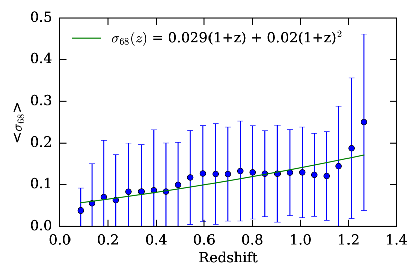
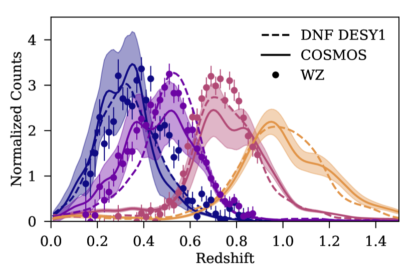
| Value | Bin 1 | Bin 2 | Bin 3 | Bin 4 |
|---|---|---|---|---|
| range | 0.20–0.43 | 0.43–0.63 | 0.63–0.90 | 0.90-1.30 |
| COSMOS footprint sampling | ||||
| COSMOS limited sample size | ||||
| COSMOS photometric calibration errors | ||||
| COSMOS hidden variables | ||||
| COSMOS errors in matching | ||||
| COSMOS single-bin uncertainty | ||||
| metacalibration | ||||
| COSMOS final , tomographic uncertainty | ||||
| WZ final | — | |||
| Combined final | ||||
Affiliations
1 Universitäts-Sternwarte, Fakultät für Physik, Ludwig-Maximilians Universität München, Scheinerstr. 1, 81679 München, Germany
2 Max Planck Institute for Extraterrestrial Physics, Giessenbachstrasse, 85748 Garching, Germany
3 Kavli Institute for Particle Astrophysics & Cosmology, P. O. Box 2450, Stanford University, Stanford, CA 94305, USA
4 SLAC National Accelerator Laboratory, Menlo Park, CA 94025, USA
5 Department of Physics and Astronomy, University of Pennsylvania, Philadelphia, PA 19104, USA
6 Centro de Investigaciones Energéticas, Medioambientales y Tecnológicas (CIEMAT), Madrid, Spain
7 Department of Physics & Astronomy, University College London, Gower Street, London, WC1E 6BT, UK
8 Department of Physics, ETH Zurich, Wolfgang-Pauli-Strasse 16, CH-8093 Zurich, Switzerland
9 Institute of Space Sciences, IEEC-CSIC, Campus UAB, Carrer de Can Magrans, s/n, 08193 Barcelona, Spain
10 Department of Physics, Stanford University, 382 Via Pueblo Mall, Stanford, CA 94305, USA
11 Center for Cosmology and Astro-Particle Physics, The Ohio State University, Columbus, OH 43210, USA
12 Department of Physics, The Ohio State University, Columbus, OH 43210, USA
13 Institut de Física d’Altes Energies (IFAE), The Barcelona Institute of Science and Technology, Campus UAB, 08193 Bellaterra (Barcelona) Spain
14 Brookhaven National Laboratory, Bldg 510, Upton, NY 11973, USA
15 ARC Centre of Excellence for All-sky Astrophysics (CAASTRO)
16 School of Mathematics and Physics, University of Queensland, Brisbane, QLD 4072, Australia
17 Laboratório Interinstitucional de e-Astronomia - LIneA, Rua Gal. José Cristino 77, Rio de Janeiro, RJ - 20921-400, Brazil
18 Observatório Nacional, Rua Gal. José Cristino 77, Rio de Janeiro, RJ - 20921-400, Brazil
19 INAF - Osservatorio Astrofisico di Torino, Pino Torinese, Italy
20 Department of Astronomy, University of Illinois, 1002 W. Green Street, Urbana, IL 61801, USA
21 National Center for Supercomputing Applications, 1205 West Clark St., Urbana, IL 61801, USA
22 Kavli Institute for Cosmological Physics, University of Chicago, Chicago, IL 60637, USA
23 School of Physics and Astronomy, University of Southampton, Southampton, SO17 1BJ, UK
24 Fermi National Accelerator Laboratory, P. O. Box 500, Batavia, IL 60510, USA
25 Centre for Astrophysics & Supercomputing, Swinburne University of Technology, Victoria 3122, Australia
26 Lawrence Berkeley National Laboratory, 1 Cyclotron Road, Berkeley, CA 94720, USA
27 Australian Astronomical Observatory, North Ryde, NSW 2113, Australia
28 Sydney Institute for Astronomy, School of Physics, A28, The University of Sydney, NSW 2006, Australia
29 Department of Astronomy, The Ohio State University, Columbus, OH 43210, USA
30 The Research School of Astronomy and Astrophysics, Australian National University, ACT 2601, Australia
31 Institute of Cosmology & Gravitation, University of Portsmouth, Portsmouth, PO1 3FX, UK
32 Jodrell Bank Center for Astrophysics, School of Physics and Astronomy, University of Manchester, Oxford Road, Manchester, M13 9PL, UK
33 Department of Physics, University of Arizona, Tucson, AZ 85721, USA
34 Purple Mountain Observatory, Chinese Academy of Sciences, Nanjing, Jiangshu 210008, China
35 Cerro Tololo Inter-American Observatory, National Optical Astronomy Observatory, Casilla 603, La Serena, Chile
36 Department of Physics and Electronics, Rhodes University, PO Box 94, Grahamstown, 6140, South Africa
37 LSST, 933 North Cherry Avenue, Tucson, AZ 85721, USA
38 CNRS, UMR 7095, Institut d’Astrophysique de Paris, F-75014, Paris, France
39 Sorbonne Universités, UPMC Univ Paris 06, UMR 7095, Institut d’Astrophysique de Paris, F-75014, Paris, France
40 George P. and Cynthia Woods Mitchell Institute for Fundamental Physics and Astronomy, and Department of Physics and Astronomy, Texas A&M University, College Station, TX 77843, USA
41 Department of Physics, IIT Hyderabad, Kandi, Telangana 502285, India
42 Department of Physics, California Institute of Technology, Pasadena, CA 91125, USA
43 Jet Propulsion Laboratory, California Institute of Technology, 4800 Oak Grove Dr., Pasadena, CA 91109, USA
44 Department of Astronomy, University of Michigan, Ann Arbor, MI 48109, USA
45 Department of Physics, University of Michigan, Ann Arbor, MI 48109, USA
46 Instituto de Fisica Teorica UAM/CSIC, Universidad Autonoma de Madrid, 28049 Madrid, Spain
47 Institute of Astronomy, University of Cambridge, Madingley Road, Cambridge CB3 0HA, UK
48 Kavli Institute for Cosmology, University of Cambridge, Madingley Road, Cambridge CB3 0HA, UK
49 Department of Astronomy, University of California, Berkeley, 501 Campbell Hall, Berkeley, CA 94720, USA
50 Astronomy Department, University of Washington, Box 351580, Seattle, WA 98195, USA
51 Santa Cruz Institute for Particle Physics, Santa Cruz, CA 95064, USA
52 Argonne National Laboratory, 9700 South Cass Avenue, Lemont, IL 60439, USA
53 Departamento de Física Matemática, Instituto de Física, Universidade de São Paulo, CP 66318, São Paulo, SP, 05314-970, Brazil
54 Department of Astrophysical Sciences, Princeton University, Peyton Hall, Princeton, NJ 08544, USA
55 Institució Catalana de Recerca i Estudis Avançats, E-08010 Barcelona, Spain
56 Department of Physics and Astronomy, Pevensey Building, University of Sussex, Brighton, BN1 9QH, UK
57 Instituto de Física, UFRGS, Caixa Postal 15051, Porto Alegre, RS - 91501-970, Brazil
58 Instituto de Física Gleb Wataghin, Universidade Estadual de Campinas, 13083-859, Campinas, SP, Brazil
59 Computer Science and Mathematics Division, Oak Ridge National Laboratory, Oak Ridge, TN 37831
60 Excellence Cluster Universe, Boltzmannstr. 2, 85748 Garching, Germany
61 Institute for Astronomy, University of Edinburgh, Edinburgh EH9 3HJ, UK