Focusing RKKY interaction by graphene P-N junction

Abstract

The carrier-mediated RKKY interaction between local spins plays an important role for the application of magnetically doped graphene in spintronics and quantum computation. Previous studies largely concentrate on the influence of electronic states of uniform systems on the RKKY interaction. Here we reveal a very different way to manipulate the RKKY interaction by showing that the anomalous focusing – a well-known electron optics phenomenon in graphene P-N junctions – can be utilized to refocus the massless Dirac electrons emanating from one local spin to the other local spin. This gives rise to rich spatial interference patterns and symmetry-protected non-oscillatory RKKY interaction with a strongly enhanced magnitude. It may provide a new way to engineer the long-range spin-spin interaction in graphene.

I Introduction

Graphene Castro Neto et al. (2009), a single atomic layer of graphite, is featured by ultra-high mobility and electrical tunability of carrier density and hence provides an attractive platform for studying the unique electron optics of Dirac fermions owing to its gapless and linear dispersion. Cheianov et al. Cheianov et al. (2007) proposed the interesting idea that an interface between electron (N)-doped and hole (P)-doped regions in graphene can focus an electron beam, which may lead to the realization of an electronic analog of the Veselago lens in optics Veselago (1968); Pendry (2000); Zhang and Liu (2008); Pendry et al. (2012). This anomalous focusing effect has motivated many new ideas and device concepts Cserti et al. (2007); Garcia-Pomar et al. (2008); Moghaddam and Zareyan (2010); Silveirinha and Engheta (2013); Zhao et al. (2013). Very recently, this effect was observed experimentally Lee et al. (2015); Chen et al. (2016), which paves the way for realizing electron optics based on graphene P-N junctions (PNJs). A common feature of these works is that they concentrate on focusing the electrons themselves, leaving its potential applications to other fields unexplored.

In this work, we explore a very different direction by showing that the anomalous focusing effect could be utilized to manipulate the carrier-mediated Rudermann-Kittel-Kasuya-Yosida (RKKY) interaction Ruderman and Kittel (1954); Kasuya (1956); Yosida (1957) between magnetic moments (spins), with potential applications in spintronics Wolf et al. (2001); Zutic et al. (2004); MacDonald et al. (2005), scalable quantum computation Loss and DiVincenzo (1998); Trifunovic et al. (2012), and majorana fermion physics Klinovaja et al. (2013) as the RKKY interaction enables long-range correlation between spatially separated local spins Piermarocchi et al. (2002); Craig et al. (2004); Rikitake and Imamura (2005); Friesen et al. (2007); Srinivasa et al. (2015), a crucial ingredient in these developments. In recent years, a lot of efforts have been devoted to characterizing the RKKY interaction in different 2D uniform systems such as two-dimensional electron gases Fischer and Klein (1975); Béal-Monod (1987), graphene Brey et al. (2007); Saremi (2007); Black-Schaffer (2010a); Sherafati and Satpathy (2011a, b); Uchoa et al. (2011); Kogan (2011), and the surface of topological insulators Liu et al. (2009); Zhu et al. (2011); Abanin and Pesin (2011). There are also many interesting schemes to manipulate the RKKY interaction Inosov et al. (2009); Zhu et al. (2010); Néel et al. (2011); Yao et al. (2014); Holub et al. (2004); Xiu et al. (2010); Nie et al. (2016); Bouhassoune et al. (2014); Power et al. (2012). Recent experimental advances further enable the RKKY interaction to be mapped out with atomic-scale resolution from single-atom magnetometry using scanning tunnelling spectroscopy Meier et al. (2008); Zhou et al. (2010); Khajetoorians et al. (2012). However, in a $d$-dimensional uniform system, the RKKY interaction usually decays at least as fast as $1/R^{d}$. This rapid decay – a common feature of the previous studies mentioned above – makes the RKKY interaction very short-ranged and may hinder its applications. This motivates growing interest in modifying the long-range behavior of the RKKY interaction, e.g., the $1/R^{3}$ long-range decay in undoped graphene can be changed by thermal excitation Klier et al. (2015) and even be slowed down by electron-electron interactions Black-Schaffer (2010b). Here we show that the graphene PNJ allows the diverging electron beams emanating from one local spin to be refocused onto the other local spin, thus the electron-mediated RKKY interaction between these two local spins can be strongly enhanced and tuned beyond the $1/R^{d}$ limit of non-interacting uniform systems. The graphene PNJ also gives rise to symmetry-protected non-oscillatory RKKY interaction as a function of the distance, in sharp contrast to the “universal” oscillation of the RKKY interaction in uniform systems with a finite carrier concentration. This may provide a new way for engineering the correlation between spatially separated local spins for their applications in spintronics and quantum computation.

This paper is organized as follows. In Sec. II, we explain intuitively how to utilize the graphene PNJ to manipulate the RKKY interaction and highlight the symmetry-protected non-oscillatory RKKY interaction. Then in Sec. III, we perform numerical simulation based on the tight-binding model to demonstrate this all-electrical manipulation and discuss the experimental feasibility. Finally, we present a brief summary in Sec. IV.

II RKKY  interaction in graphene P-N junction: physical picture

Let us consider two local spins $\hat{\mathbf{S}}_{1}$ (located at $\mathbf{R}_{1}$) and $\hat{\mathbf{S}}_{2}$ (located at $\mathbf{R}_{2}$) coupled to the spin density $\hat{\mathbf{s}}(\mathbf{x})\equiv\hat{\mathbf{s}}\delta(\hat{\mathbf{r}}-\mathbf{x})$ of itinerant carriers via the exchange interaction $\hat{V}_{\mathrm{ex}}=-J_{0}\hat{\mathbf{S}}_{1}\cdot\hat{\mathbf{s}}(\mathbf{R}_{1})-J_{0}\hat{\mathbf{S}}_{2}\cdot\hat{\mathbf{s}}(\mathbf{R}_{2}),$ where $\hat{\mathbf{s}}$ ($\hat{\mathbf{r}}$) is the carrier spin (position) operator. The total Hamiltonian of the coupled system is the sum of $\hat{V}_{\mathrm{ex}}$ and the carrier Hamiltonian $\hat{H}$. The carrier-mediated RKKY interaction originates from the local excitation of carrier spin density fluctuation by one local spin and its subsequent propagation to the other spin. At zero temperature, the effective RKKY interaction between the local spins is obtained by eliminating the carrier degree of freedom through second-order perturbation theory as Ruderman and Kittel (1954); Kasuya (1956); Yosida (1957); Bruno (1995) $\hat{H}_{\mathrm{RKKY}}=\sum_{\alpha\beta=x,y,z}J_{\alpha\beta}\hat{S}_{1}^{\alpha}\hat{S}_{2}^{\beta}$, where the RKKY range function

$$J_{\alpha\beta}=-\frac{J_{0}^{2}}{\pi}\int_{-\infty}^{E_{F}}\operatorname{Im}\mathrm{Tr}[\hat{s}_{\alpha}\hat{G}(\mathbf{R}_{1},\mathbf{R}_{2};E)\hat{s}_{\beta}\hat{G}(\mathbf{R}_{2},\mathbf{R}_{1};E)]dE,$$ (1)

$E_{F}$ is the Fermi energy of the carriers, $\mathrm{Tr}$ traces over the carrier spin, and $\hat{G}(\mathbf{r},{\mathbf{r}}_{0};E)\equiv\langle\mathbf{r}|(E+i0^{+}-\hat{H})|\mathbf{r}_{0}\rangle$ is the unperturbed (i.e., in the absence of the local spins) propagator of the carriers in real space. In general, $\hat{G}(\mathbf{r},{\mathbf{r}}_{0};E)$ is still an operator acting on the carrier spin degree of freedom. In a $d$-dimensional uniform system, the carriers excited by the first local spin at $\mathbf{R}_{1}$ propagate towards the second local spin at $\mathbf{R}_{2}$ in the form of an outgoing wave $\hat{G}({\mathbf{R}_{2}},{\mathbf{R}_{1}},E)\sim e^{ikR}/R^{(d-1)/2}$, where $R\equiv|\mathbf{R}_{2}-\mathbf{R}_{1}|$, $k$ is a characteristic wave vector of the carriers with energy $E$, and the denominator $R^{(d-1)/2}$ ensures the conservation of probability current. The integration over the energy in Eq. (1) yields another factor $1/R$ from the oscillating phase factor $e^{ikR}$, so $J_{\alpha\beta}\propto 1/R^{d}$. This provides a rough explanation for the “universal” $1/R^{d}$ decay of the RKKY interaction, as discovered in a great diversity of materials by previous studies. It also reveals a very different way – tailoring the carrier propagation and interference – to manipulate the RKKY interaction beyond this constraint, as opposed to previous studies that exploit the electronic states and energy band structures of different uniform materials. The anomalous focusing effect in graphene PNJs Cheianov et al. (2007) provides a paradigmatic example for this manipulation.

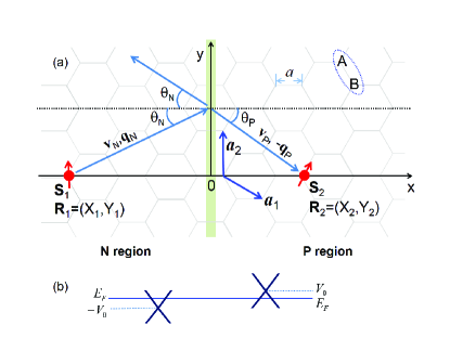
Figure 1: (a) Graphene P-N junction at $x=0$, with two localized spins $\mathbf{S}_{1}$ (in the N region) and $\mathbf{S}_{2}$ (in the P region). The unit cell of graphene (dashed ellipse) consists of one atom on sublattice $A$ and one atom on sublattice $B$. (b) Dirac cones of the N region and P region relative to the Fermi energy. $\mathbf{v}_{\mathrm{N}}\parallel\mathbf{q}_{N}$ and $\mathbf{v}_{\mathrm{P}}\parallel(-\mathbf{q}_{P})$ are the group velocities of the incident and transmission waves, respectively.

As shown in Fig. 1(a), the honeycomb lattice of graphene consists of two sublattices (denoted by $A$ and $B$) and each unit cell contains two carbon atoms (or $\pi_{z}$-orbitals), one on each sublattice. Let us use $\mathbf{R}$ to denote the location of each carbon atom, $|\mathbf{R}\rangle$ for the corresponding orbital, and $s_{\mathbf{R}}$ ($=A$ or $B$) for the sublattice on which $\mathbf{R}$ locates. For carriers in the graphene PNJ, the tight-binding Hamiltonian is the sum of $\hat{H}_{0}$ for uniform graphene and $\hat{V}_{\mathrm{J}}$ for the on-site junction potential:

$$\hat{H} =\hat{H}_{0}+\hat{V}_{\mathrm{J}},$$ (2a)

$$\hat{H}_{0} =-t\sum_{\langle\mathbf{R},\mathbf{R}^{\prime}\rangle}|\mathbf{R}\rangle\langle\mathbf{R}^{\prime}|+h.c.,$$ (2b)

$$\hat{V}_{\mathrm{J}} =\sum_{\mathbf{R}}V_{\mathbf{R}}|\mathbf{R}\rangle\langle\mathbf{R}|,$$ (2c)

where $$\langle\mathbf{R},\mathbf{R}^{\prime}\rangle t\approx 3 V_{\mathbf{R}} -V_{0} +V_{0} \mathbf{R} V_{0}\geq 0 -V_{0} +V_{0} V_{0}=0 V_{0} E_{F}>V_{0} E_{F}<V_{0} E_{F}\in[-V_{0},+V_{0}] (V_{0}=0 E_{F} V_{0}+E_{F} V_{0}-E_{F} E_{F}=0$$ denotes nearest neighbors, eV is the nearest-neighbor hopping Castro Neto et al. (2009), and is equal to () when locates in the left (right) of the junction [shaded stripe in Fig. 1(a)] with . As shown in Fig. 1(b), the zero point of energy is chosen such that the Dirac point in the left (right) of the junction lies at (). Uniform graphene corresponds to , while nonzero corresponds to a junction, e.g., N-N (P-P) junction corresponds to (). Here we consider the P-N junction (PNJ), corresponding to . In uniform graphene ), the doping is determined by . In graphene PNJ, the electron doping in the N region (left) is , while the hole doping in the P region (right) is , e.g., corresponds to the electron doping in the N region being equal to the hole doping in the P region.

Due to the absence of spin-orbit coupling in the carrier Hamiltonian $\hat{H}$, the carrier-mediated RKKY interaction at zero temperature between one local spin $\hat{\mathbf{S}}_{1}$ at $\mathbf{R}_{1}$ (sublattice $s_{\mathbf{R}_{1}}$) in the N region and another local spin $\hat{\mathbf{S}}_{2}$ at $\mathbf{R}_{2}$ (sublattice $s_{\mathbf{R}_{2}}$) in the P region [see Fig. 1(a)] assumes the isotropic Heisenberg form Sherafati and Satpathy (2011a, b): $\hat{H}_{\mathrm{RKKY}}=J\hat{\mathbf{S}}_{1}\cdot\hat{\mathbf{S}}_{2}$, where the range function

$$J=-\frac{J_{0}^{2}}{2\pi}\int_{-\infty}^{E_{F}}\operatorname{Im}G^{2}(\mathbf{R}_{2},\mathbf{R}_{1},E)dE$$ (3)

is determined by the unperturbed propagator (i.e., in the absence of the local spins) of the carriers from $\mathbf{R}_{1}$ to $\mathbf{R}_{2}$:

$$G(\mathbf{R}_{2},\mathbf{R}_{1},E)\equiv\langle\mathbf{R}_{2}|(E+i0^{+}-\hat{H})|\mathbf{R}_{1}\rangle.$$

In arriving at Eq. (3), we have used $G(\mathbf{R}_{2},\mathbf{R}_{1},E)=G(\mathbf{R}_{1},\mathbf{R}_{2},E)$ due to the time-reversal invariance of the graphene Hamiltonian $\hat{H}$. Note that the propagator $G(\mathbf{R}_{2},\mathbf{R}_{1},E)$ and hence the RKKY range function $J$ are very sensitive to the sublattices on which $\mathbf{R}_{1}$ and $\mathbf{R}_{2}$ locate (i.e., $s_{\mathbf{R}_{1}}$ and $s_{\mathbf{R}_{2}}$), e.g., when $\mathbf{R}_{2}$ moves from an atom on the $A$ sublattice ($s_{\mathbf{R}_{2}}=A$) to a neighboring atom on the $B$ sublattice ($s_{\mathbf{R}_{2}}=B$) [see Fig. 1(a)], the propagator and hence the RKKY interaction may change significantly.

Now we discuss how the anomalous focusing effect in graphene PNJs Cheianov et al. (2007) can be utilized to manipulate the carrier propagator and hence the RKKY interaction beyond the “universal” $1/R^{d}$ long-range decay as encountered in previous studies. Ever since the pioneering work of Cheianov et al. Cheianov et al. (2007), there have been many studies on the anomalous focusing effect, either based on the classical analogy to light propagation in geometric optics or based on the scattering of the electron wave functions. Below, we provide a physically intuitive analysis on how the graphene PNJ focuses the carrier propagator and hence the RKKY interaction based on the continuum model of graphene Castro Neto et al. (2009). The purpose is to provide a qualitative picture for the focusing of the RKKY interaction and establish its effectiveness for an arbitrary direction of the P-N interface.

II.1 Anomalous focusing of carrier propagator: continuum model

The low-energy physics of graphene is described by two Dirac cones located at $\mathbf{K}$ and $\mathbf{K}^{\prime}=-\mathbf{K}$, which form a Kramer pair. For clarity, we first analyze the focusing effect based on the $\mathbf{K}$-valley continuum model, leaving the discussion including both valleys to the end of this subsection. Using the band-edge Bloch functions $|\Phi_{\mathbf{K},A}\rangle$ (from $\pi_{z}$-orbitals on the $A$ sublattice) and $|\Phi_{\mathbf{K},B}\rangle$ (from $\pi_{z}$-orbitals on the $B$ sublattice) of the $\mathbf{K}$ valley as the basis, the continuum model for the $\mathbf{K}$ valley reads Castro Neto et al. (2009),

$$\hat{h}=v_{F}\boldsymbol{\hat{\sigma}}\cdot\mathbf{\hat{p}}+\mathrm{sgn}(x)V_{0},$$ (4)

where $\mathbf{\hat{p}}$ is the momentum relative to the $\mathbf{K}$ valley and $v_{F}$ is the Fermi velocity. Note that the continuum model regards the two atoms of the same unit cell to locate at the same spatial point, so each spatial point contains two sublattices/orbitals and the Hamiltonian $\hat{h}$ is a $2\times 2$ matrix. Correspondingly, the carrier propagator from $\mathbf{R}_{1}$ to $\mathbf{R}_{2}$ is also a 2$\times$2 matrix: $\mathbf{g}(\mathbf{R}_{2},\mathbf{R}_{1},E)\equiv\langle\mathbf{R}_{2}|(E+i0^{+}-\hat{h})|\mathbf{R}_{1}\rangle$, e.g., its $(B,A)$ matrix element gives the carrier propagator from the sublattice $A$ at $\mathbf{R}_{1}$ to the sublattice $B$ at $\mathbf{R}_{2}$.

For uniform graphene, the $\mathbf{K}$-valley continuum model [Eq. (4) with $V_{0}=0$] leads to a massless Dirac spectrum $E_{\pm}(\mathbf{q})\equiv\pm v_{F}|\mathbf{q|}$ and chiral eigenstates $|\pm,\mathbf{q}\rangle=e^{i\mathbf{q}\cdot\mathbf{r}}|u_{\pm}(\mathbf{q})\rangle$, where $|u_{\pm}(\mathbf{q})\rangle$ is the two-component spinor for the sublattice degrees of freedom. The conduction (valence) band state $|+,\mathbf{q}\rangle$ ($|-,\mathbf{q}\rangle$) has a group velocity $\mathbf{v}(\mathbf{q})=v_{F}\mathbf{q}/|\mathbf{q}|$ [$-\mathbf{v}(\mathbf{q})\equiv-v_{F}\mathbf{q}/|\mathbf{q}|$] parallel (anti-parallel) to the momentum $\mathbf{q}$. The RKKY interaction is usually dominated by the contributions from carriers near the Fermi surface [the energy integral in Eq. (3) merely produces a multiplicative factor $\propto 1/R$], so we focus on the carrier propagator on the Fermi level $E_{F}$. For $E_{F}>0$, the Fermi momentum is $q_{F}\equiv E_{F}/v_{F}$, and the right-going eigenstates $|+,\mathbf{q}\rangle$ on the Fermi contour are characterized by the momentum $\mathbf{q}\equiv((q_{F}^{2}-q_{y}^{2})^{1/2},q_{y})$. The 2$\times$2 propagator from $\mathbf{R}_{1}$ to $\mathbf{R}_{2}$ (on the right of $\mathbf{R}_{1}$) in uniform graphene can be expressed in terms of these eigenstates as

$$\mathbf{g}_{\mathrm{uniform}}(\mathbf{R}_{2},\mathbf{R}_{1},E_{F})=\int_{-\infty}^{\infty}\frac{dq_{y}}{2\pi}\frac{|u_{+}(\mathbf{q})\rangle\langle u_{+}(\mathbf{q})|}{iv_{x}(\mathbf{q})}e^{i\mathbf{q}\cdot(\mathbf{R}_{2}-\mathbf{R}_{1})}.$$ (5)

The RKKY interaction in uniform graphene is given by Eq. (3) with $G(\mathbf{R}_{2},\mathbf{R}_{1},E)$ replaced by the $(s_{\mathbf{R}_{2}},s_{\mathbf{R}_{1}})$ matrix element of $\mathbf{g}_{\mathrm{uniform}}(\mathbf{R}_{2},\mathbf{R}_{1},E_{F})$.

For the graphene PNJ described by the $\mathbf{K}$-valley continuum model in Eq. (4), the first local spin $\mathbf{S}_{1}$ in the N region excites a series of outgoing plane wave eigenstates on the Fermi contour, but only the right-going eigenstates, i.e., $|+,\mathbf{q}_{N}\rangle$ with momentum $\mathbf{q}_{N}\equiv((q_{N}^{2}-q_{y}^{2})^{1/2},q_{y})$, can transmit across the P-N interface, becomes a right-going eigenstate $|-,\mathbf{q}_{P}\rangle$ with momentum $\mathbf{q}_{P}\equiv(-(q_{P}^{2}-q_{y}^{2})^{1/2},q_{y})$ on the Fermi contour of the P region, and finally arrive at $\mathbf{S}_{2}$, where $q_{N}\equiv(V_{0}+E_{F})/v_{F}$ and $q_{P}\equiv(V_{0}-E_{F})/v_{F}$ are Fermi momenta in the N and P regions, respectively. In terms of these local, right-going eigenstates on the Fermi contours, the carrier propagator from $\mathbf{R}_{1}$ to $\mathbf{R}_{2}$ is (see Appendix A):

$$\mathbf{g}(\mathbf{R}_{2},\mathbf{R}_{1},E)=\int_{-\infty}^{\infty}\frac{dq_{y}}{2\pi}w(q_{y})\frac{|u_{-}(\mathbf{q}_{P})\rangle\langle u_{+}(\mathbf{q}_{N})|}{iv_{x}(\mathbf{q}_{N})}e^{i\mathbf{q}_{P}\cdot\mathbf{R}_{2}}e^{-i\mathbf{q}_{N}\cdot\mathbf{R}_{1}},$$ (6)

where $w(q_{y})$ is the transmission coefficient of the incident state $|+,\mathbf{q}_{N}\rangle$ across the PNJ. The RKKY interaction in the graphene PNJ is given by Eq. (3) with $G(\mathbf{R}_{2},\mathbf{R}_{1},E)$ replaced by the $(s_{\mathbf{R}_{2}},s_{\mathbf{R}_{1}})$ matrix element of $\mathbf{g}(\mathbf{R}_{2},\mathbf{R}_{1},E_{F})$.

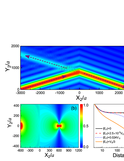
Figure 2: Anomalous focusing across a graphene PNJ at $x=0$. The propagator is the sum of the contributions from all the wave packets characterized by different center momenta on the Fermi contour. (a) Contribution of a single wave packet on the Fermi contour (whose center momentum has an incident angle $\theta_{N}=15\operatorname{{{}^{\circ}}}$) to the propagator $|g_{BA}(\mathbf{R}_{2},\mathbf{R}_{1},E_{F}=0.03t)|$ vs. $\mathbf{R}_{2}=(X_{2},Y_{2})$ on the $B$ sublattice, where $\mathbf{R}_{1}=(X_{1},Y_{1})$ is fixed at $X_{1}=-3000a$ and $Y_{1}=0$ on the $A$ sublattice. The dashed arrows mark the classical trajectory. (b) Propagator $|g_{BA}(\mathbf{R}_{2},\mathbf{R}_{1},E_{F}=0)|$ vs. $\mathbf{R}_{2}$ on $B$ sublattice for fixed $\mathbf{R}_{1}=(-601a,0)$ on $A$ sublattice. (c) Decay of the propagator $|g_{BA}(\mathbf{R}_{2},\mathbf{R}_{1},E_{F})|$ along the $x$ axis (i.e., $Y_{1}=Y_{2}=0$) with increasing distance $R$, where $\mathbf{R}_{2}$ is on the cusp of the caustics. The PNJ potential $V_{0}=t/2$ for (a) and $t/5$ for (b) and (c).

The key difference between the carrier propagator in the graphene PNJ [Eq. (6)] and that in uniform graphene [Eq. (5)] is the change of the propagation phase factor from $e^{i\mathbf{q}\cdot(\mathbf{R}_{2}-\mathbf{R}_{1})}\equiv e^{i\phi_{0}(q_{y})}$ for uniform graphene to $e^{i(\mathbf{q}_{P}\cdot\mathbf{R}_{2}-\mathbf{q}_{N}\cdot\mathbf{R}_{1})}\equiv e^{i\phi_{\mathrm{NP}}(q_{y})}$ for the graphene PNJ. This change is responsible for the anomalous focusing of the diverging carrier wave into a converging one. For an intuitive analysis of this behavior, we discretize the $q_{y}$ axis into grids $m\Delta$ ($m\in\mathbb{Z}$), where the spacing $\Delta\ll$ size of the graphene Brillouin zone. Then Eq. (6) gives $\mathbf{g}(\mathbf{R}_{2},\mathbf{R}_{1},E)=\sum_{m}\mathbf{g}^{(m)}(\mathbf{R}_{2},\mathbf{R}_{1},E)$ and $\mathbf{g}^{(m)}$ is the contribution from the $q_{y}$ integral over the $m$th segment $[(m-1/2)\Delta,(m+1/2)\Delta]$, corresponding to a wave packet characterized by the center momentum $q_{y}=m\Delta$. In other words, the entire propagator is the sum of contributions from all these wave packets characterized by different center momenta $q_{y}$’s on the Fermi contour. The same analysis is applicable to the propagator $\mathbf{g}_{\mathrm{uniform}}$ in uniform graphene [Eq. (5)]. Since the integrand is the product of a slowly-varying part and a rapidly oscillating propagation phase factor, the contribution from a given wave packet characterized by the center momentum $q_{y}$ is appreciable only when the propagation phase is stationary:$\ \partial_{q_{y}}\phi_{0}(q_{y})=0$ (for uniform graphene) or $\partial_{q_{y}}\phi_{\mathrm{NP}}(q_{y})=0$ (for graphene PNJ). This first-order stationary phase condition determines the most probable (or classical) trajectory of a wave packet emanating from $\mathbf{R}_{1}$.

In uniform graphene, the classical trajectory of a given wave packet characterized by the center momentum $\mathbf{q}=((q_{F}^{2}-q_{y}^{2})^{1/2},q_{y})$ on the Fermi contour [Eq. (5)] is a beam emanating from $\mathbf{R}_{1}$ and going along the wave vector $\mathbf{q}$. The classical trajectories of different wave packets on the Fermi contour form many outgoing beams emanating from $\mathbf{R}_{1}$, which manifests the diverging propagation of the carriers in uniform graphene and leads to $\mathbf{g}_{\mathrm{uniform}}\propto 1/R^{1/2}$. By contrast, in the graphene PNJ, the classical trajectory of a given wave packet characterized by the center momentum $\mathbf{q}_{N}=((q_{N}^{2}-q_{y}^{2})^{1/2},q_{y})$ with incident angle $\theta_{N}=\tan^{-1}(q_{y}/q_{N,x})$ consists of the incident beam along $\mathbf{q}_{N}$, the reflection beam with a reflection angle $\theta_{N}$, and the refraction beam with a refraction angle $\theta_{P}\equiv\tan^{-1}(q_{y}/q_{P,x})$, as sketched in Fig. 1(a) and further visualized in Fig. 2(a). Here the refraction angle $\theta_{P}$ is determined by the Snell law $\sin\theta_{N}=n\sin\theta_{P}$ with a negative effective refractive index $n\equiv-(V_{0}-E_{F})/(V_{0}+E_{F})$ Cheianov et al. (2007).

Let us use $(X_{1},Y_{1})$ and $(X_{2},Y_{2})$ to denote the Cartesian coordinates of $\mathbf{R}_{1}$ and $\mathbf{R}_{2}$, respectively. In the graphene PNJ, when $\mathbf{R}_{2}$ locates on the caustics Cheianov et al. (2007)

$$(Y_{2}-Y_{1})^{2}=\frac{[X_{2}^{2/3}-(nX_{1})^{2/3}]^{3}}{n^{2}-1},$$ (7)

the wave packet going from $\mathbf{R}_{1}$ to $\mathbf{R}_{2}$ obeys not only $\partial_{q_{y}}\phi_{0}(q_{y})=0$, but also $\partial_{q_{y}}^{2}\phi_{0}(q_{y})=0$, so that its contribution to the propagator $\mathbf{g}(\mathbf{R}_{2},\mathbf{R}_{1},E_{F})$ is enhanced. The most interesting case occurs at $E_{F}=0$ or equivalently $n=-1$. In this case, we have $q_{N,x}=-q_{P,x}$, thus for $\mathbf{R}_{2}$ at the mirror image of $\mathbf{R}_{1}$ about the PNJ, i.e., $\mathbf{R}_{2}=\mathbf{R}_{1}^{\mathrm{m}}\equiv(|X_{1}|,Y_{1})$, the phase $\phi_{\mathrm{NP}}(q_{y})$ vanishes for all $q_{y}$, so that the integrand in Eq. (6) no longer suffers from the rapidly oscillating phase factor $e^{i\phi_{\mathrm{NP}}(q_{y})}$. This corresponds to constructive interference of all the transmission waves at $\mathbf{R}_{1}^{\mathrm{m}}$ or equivalently perfect focusing of the diverging electron beams emanating from $\mathbf{R}_{1}$ onto $\mathbf{R}_{1}^{\mathrm{m}}$ Cheianov et al. (2007). This not only lead to strong local enhancement of the propagator $\mathbf{g}(\mathbf{R}_{2},\mathbf{R}_{1},E_{F}=0)$ when $\mathbf{R}_{2}$ locates in the vicinity of $\mathbf{R}_{1}^{\mathrm{m}}$ [see Fig. 2(b)], but also makes $\mathbf{g}(\mathbf{R}_{1}^{\mathrm{m}},\mathbf{R}_{1},E_{F}=0)$ independent of the distance $R$ [black, solid line in Fig. 2(c)], in sharp contrast to the $1/R^{1/2}$ decay in uniform graphene. This distance independent propagator can be attributed to the existence of a hidden symmetry on the Fermi contours of the host material Zhang et al. (2016).

When $E_{F}\neq 0$, the anomalous focusing locally enhances the propagator from $\mathbf{R}_{1}$ to its caustics and slows down its decay with the distance to a slower rate $\sim 1/R^{\xi}$ ($\xi<1/2$) compared with the $1/R^{1/2}$ decay in uniform graphene, as a consequence of imperfect focusing away from $n=-1$, e.g., for $\mathbf{R}_{2}$ on the cusp $(|nX_{1}|,0),$ we have $\xi\approx 0.24$ nearly independent of $E_{F}$, as shown in Fig. 2(c). By contrast, for $\mathbf{R}_{2}$ far away from the caustics, the propagator recovers the $1/R^{1/2}$ decay of uniform graphene. In addition to locally enhancing the propagator, the PNJ also slightly decreases the propagation amplitude via the finite transmission $w(q_{y})$. However, this effect is of minor importance because Klein tunneling Katsnelson et al. (2006) allows carriers with a small incident angle $\theta_{N}$ to go through the PNJ almost completely, as demonstrated by the weak reflection in Fig. 2(a) when the incident angle is small.

From the above analysis, it is clear that the PNJ qualitatively changes the diverging spherical propagation of carriers in graphene into a converging one. This greatly enhances the propagator near the caustics, so that its decay with inter-spin distance $R$ slows down (for $E_{F}\neq 0$) and even ceases (for $E_{F}=0$). At large distances, the non-decaying propagator could lead to $1/R$ decay of the RKKY interaction between two mirror symmetric spins about the PNJ, as we demonstrate shortly (see Sec. IIIA).

Before concluding this subsection, we emphasize that the above analysis is based on the $\mathbf{K}$-valley continuum model, featured by a single Dirac cone and a circular Fermi contour. This simplified model ignores two important effects: the trigonal warping at high energies and the presence of another Dirac cone at $\mathbf{K}^{\prime}=-\mathbf{K}$. At high Fermi energies $|E_{F}|\sim t$, the trigonal warping leads to non-circular Fermi contours, while the inter-valley scattering may decrease the transmission probability across a sharp PNJ Logemann et al. (2015). The former makes the focusing effect no longer perfect even when $E_{F}=0$, while the latter decreases the carrier propagator and hence the RKKY interaction. Even in the linear regime $|E_{F}|\ll t$, the presence of two inequivalent valleys still gives rise to inter-valley interference that significantly affect the RKKY interaction, as discussed by Sherafati and Satpathy Sherafati and Satpathy (2011a, b) for uniform graphene. Here we briefly discuss this issue for the graphene PNJ. First, we assume that the P-N interface does not induce inter-valley scattering. Then, when both $\mathbf{K}$ and $\mathbf{K}^{\prime}$ valleys are included, the 2$\times$2 carrier propagator from $\mathbf{R}_{1}$ to $\mathbf{R}_{2}$ would be

$$\mathbb{G}(\mathbf{R}_{2},\mathbf{R}_{1},E)=e^{i\mathbf{K}\cdot(\mathbf{R}_{2}-\mathbf{R}_{1})}\mathbf{g}(\mathbf{R}_{2},\mathbf{R}_{1},E)+e^{i\mathbf{K}^{\prime}\cdot(\mathbf{R}_{2}-\mathbf{R}_{1})}\mathbf{g}^{\prime}(\mathbf{R}_{2},\mathbf{R}_{1},E),$$

where $\mathbf{g}$ ($\mathbf{g}^{\prime}$) is the propagator in the presence of the $\mathbf{K}$ ($\mathbf{K}^{\prime}$) valley alone [see Eq. (6) for the expression of $\mathbf{g}$]. The $\mathbf{K}^{\prime}$-valley continuum model $\hat{h}^{\prime}=-v_{F}\boldsymbol{\hat{\sigma}}^{\ast}\cdot\mathbf{\hat{p}}+\mathrm{sgn}(x)V_{0}$ is the time reversal of the $\mathbf{K}$-valley model [Eq. (4)], so that $g_{s_{2}s_{1}}^{\prime}(\mathbf{R}_{2},\mathbf{R}_{1},E)=g_{s_{1}s_{2}}(\mathbf{R}_{1},\mathbf{R}_{2},E)$, i.e., the propagator of a $\mathbf{K}^{\prime}$-valley electron from the sublattice $s_{1}$ at $\mathbf{R}_{1}$ to the sublattice $s_{2}$ at $\mathbf{R}_{2}$ is equal to the propagator of a $\mathbf{K}$-valley electron from the sublattice $s_{2}$ at $\mathbf{R}_{2}$ back to the sublattice $s_{1}$ at $\mathbf{R}_{1}$. This also ensures the time-reversal invariance of the total propagator:$\ \mathbb{G}_{s_{2}s_{1}}(\mathbf{R}_{2},\mathbf{R}_{1},E)=\mathbb{G}_{s_{1}s_{2}}(\mathbf{R}_{1},\mathbf{R}_{2},E)$. The RKKY interaction is given by Eq. (3) with $G(\mathbf{R}_{2},\mathbf{R}_{1},E)$ replaced by the $(s_{\mathbf{R}_{2}},s_{\mathbf{R}_{1}})$ matrix element of $\mathbb{G}(\mathbf{R}_{2},\mathbf{R}_{1},E)$. Consequently, the RKKY interaction consists of the intra-valley contributions and the inter-valley interference term. The former oscillates slowly on the length scale of the Fermi wave length, while the latter oscillates rapidly as $e^{i(\mathbf{K-K}^{\prime})\cdot(\mathbf{R}_{2}-\mathbf{R}_{1})}$ on the atomic scale, similar to the case of uniform graphene Sherafati and Satpathy (2011a, b). In the presence of inter-valley scattering by the P-N interface, a quantitative description is very difficult within the continuum model, but we still expect the contribution from the inter-valley interference to be rapidly oscillating on the atomic scale. Therefore, the slowly-varying envelope of the RKKY interaction is always determined by the intra-valley contributions, which are independent of the direction of the P-N interface with respect to the crystalline axis of graphene. In other words, the continuum model suggests that the focusing of the RKKY interaction should occur for an arbitrary direction of the P-N interface, as confirmed by our subsequent numerical calculation based on the tight-binding model.

II.2 Symmetry-protected non-oscillatory RKKY interaction

For uniform graphene, the tight-binding Hamiltonian $\hat{H}_{0}$ [see Eq. (2a)] possesses electron-hole symmetry $\hat{P}\hat{H}_{0}\hat{P}^{-1}=-\hat{H}_{0}$. Saremi (2007); Bunder and Lin (2009); Kogan (2011), where $\hat{P}$ inverts all the $\pi_{z}$-orbitals on sublattice $B$ but keeps all $\pi_{z}$-orbitals on sublattice $A$ invariant, i.e., $\hat{P}|\mathbf{R}\rangle=\pm|\mathbf{R}\rangle$, with the upper (lower) sign for $s_{\mathbf{R}}=A$ ($s_{\mathbf{R}}=B$). For undoped graphene, this makes the RKKY interaction between local spins on the same (opposite) sublattice always ferromagnetic (antiferromagnetic), irrespective of their distance. However, once the graphene is doped, the RKKY interaction recovers its “universal” oscillation with a characteristic wavelength $\lambda_{F}/2$ ($\lambda_{F}$ is the Fermi wavelength) between ferromagnetic and anti-ferromagnetic couplings, as also found in many other materials.

For the graphene PNJ, the presence of the junction potential breaks the electron-hole symmetry of uniform graphene. Moreover, since both the N region and the P region are doped, the RKKY interaction is also expected to oscillate between ferromagnetic and antiferromagnetic couplings with the distance. Interestingly, we find that the electron-hole symmetry can be restored under certain conditions. Let us consider a general graphene PNJ described by the tight-binding Hamiltonian Eq. (2) with a general on-site junction potential $V_{\mathbf{R}}$ and define the mirror reflection operator $\hat{M}$ that maps the $\pi_{z}$-orbital $|\mathbf{R}\rangle$ to another $\pi_{z}$-orbital $|\mathbf{R}_{\mathrm{m}}\rangle$ at the mirror image location $\mathbf{R}_{\mathrm{m}}$ about the P-N interface, i.e., $\hat{M}|\mathbf{R}\rangle=|\mathbf{R}^{\mathrm{m}}\rangle$. The key observation is that as long as the mirror reflection $\hat{M}$ about the P-N interface keeps the graphene lattice invariant but inverts the junction potential (i.e., $V_{\mathbf{R}}=-V_{\mathbf{R}^{\mathrm{m}}}$), the PNJ Hamiltonian $\hat{H}$ possesses a generalized electron-hole symmetry: $(\hat{P}\hat{M})\hat{H}(\hat{P}\hat{M})^{-1}=-\hat{H}$. This ensures the eigen-energies of the PNJ to appear in pairs $(\varepsilon,-\varepsilon)$ and the corresponding eigenstates $|\phi_{\varepsilon}\rangle$ and $|\phi_{-\varepsilon}\rangle$ obey $|\phi_{-\varepsilon}\rangle=\hat{P}\hat{M}|\phi_{\varepsilon}\rangle$, similar to the electron-hole symmetry in uniform graphene Saremi (2007); Bunder and Lin (2009); Kogan (2011). As a consequence of this symmetry, when $E_{F}=0$, the Matsubara Green’s function $\mathcal{G}(\mathbf{R},\mathbf{R}^{\prime},\tau)$ Mahan (2000) obeys $\mathcal{G}(\mathbf{R}_{1},\mathbf{R}_{1}^{\mathrm{m}},-\tau)=\pm\mathcal{G}(\mathbf{R}_{1}^{\mathrm{m}},\mathbf{R}_{1},\tau)$, with the upper (lower) sign for $\mathbf{R}_{1}$ and $\mathbf{R}_{1}^{\mathrm{m}}$ on the opposite (same) sublattices. The time-reversal symmetry further dictates the Matsubara Green’s functions to be real. According to the imaginary-time formalism for the RKKY interaction Saremi (2007); Bunder and Lin (2009); Kogan (2011) [equivalent to the real-time formalism in Eq. (3)], the sign of the RKKY range function is determined by $\mathcal{G}(\mathbf{R}_{1},\mathbf{R}_{2},-\tau)\mathcal{G}(\mathbf{R}_{2},\mathbf{R}_{1},\tau)$. Therefore, when the two local spins are mirror symmetric about the PNJ, i.e., $\mathbf{R}_{2}=\mathbf{R}_{1}^{\mathrm{m}}$, their RKKY interaction is always ferromagnetic (antiferromagnetic) on the same (opposite) sublattices, irrespective of their distance. If the P-N interface is along the zigzag direction, then $\mathbf{R}_{1}$ and $\mathbf{R}_{1}^{\mathrm{m}}$ are always on opposite sublattices, so the RKKY interaction is antiferromagnetic. If the P-N interface is along the armchair direction, then $\mathbf{R}_{1}$ and $\mathbf{R}_{1}^{\mathrm{m}}$ are always on the same sublattice, so the RKKY interaction is ferromagnetic.

III Numerical results

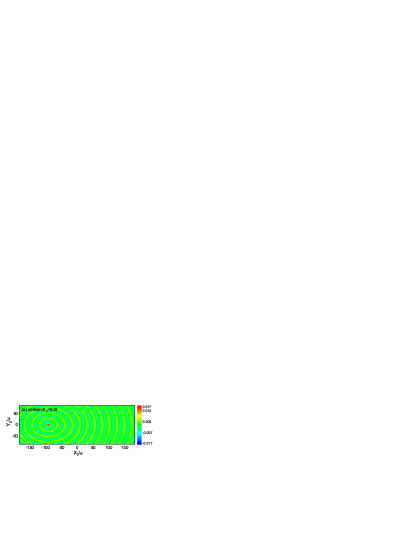
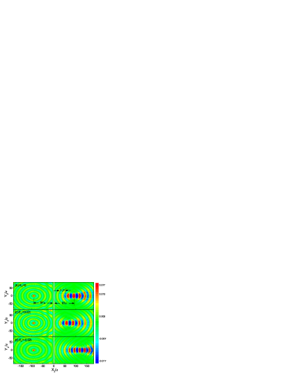
Figure 3: Scaled RKKY range function $\mathcal{J}R^{2}/a^{2}$ vs. $\mathbf{R}_{2}=(X_{2},Y_{2})$ on the $B$ sublattice for fixed $\mathbf{R}_{1}=(-91a,0)$ on the $A$ sublattice in (a) uniform graphene with electron doping $E_{F}=0.2t$ and (b)-(d) graphene PNJ with junction potential $V_{0}=0.2t$ and different Fermi energies. The same color scale is used for all the panels, i.e., blue (red) for negative (positive) or equivalently ferromagnetic (antiferromagnetic) RKKY interactions.

Here we calculate the RKKY interaction in the graphene PNJ numerically based on the tight-binding model [Eq. (2)], with the on-site junction potential $V_{\mathbf{R}}=-V_{0}$ ($V_{\mathbf{R}}=+V_{0}$) in the N (P) region. For convenience, we introduce the dimensionless RKKY range function $\mathcal{J}\equiv{tJ/J_{0}^{2}}$. Due to the transformation $\hat{H}\rightarrow-\hat{H}$ upon $(V_{0},t)\rightarrow(-V_{0},-t)$ and the time-reversal symmetry, $\mathcal{J}$ is invariant upon $(E_{F},V_{0})\rightarrow(-E_{F},-V_{0})$ (see Appendix B), so we need only consider $V_{0}>0$. Our results show that for different orientations of the PNJ (e.g., along the zigzag direction, the armchair direction, and a slightly misaligned direction) and different sublattice locations of $\mathbf{R}_{1}$ and $\mathbf{R}_{2}$, the RKKY interaction exhibits similar anomalous focusing behaviors, consistent with our previous analysis based on the continuum model in Sec. IIA. For specificity, we present our results for a PNJ along the zigzag direction and always take $\mathbf{R}_{1}$ on the $A$ sublattice and $\mathbf{R}_{2}$ on the $B$ sublattice.

III.1 Anomalous focusing of RKKY interaction

For the first local spin $\hat{\mathbf{S}}_{1}$ fixed at $\mathbf{R}_{1}=(-91a,0)$ [$a$ is the C-C bond length, see Fig. 1(a)], the spatial map of the scaled range function $\mathcal{J}R^{2}/a^{2}$ as a function of the location $\mathbf{R}_{2}=(X_{2},Y_{2})$ of the second local spin $\hat{\mathbf{S}}_{2}$ is shown in Fig. 3(a) for uniform graphene and Fig. 3(b)-(d) for graphene PNJ. Here we follow Ref. Lee et al., 2012 and use the multiplication factor $R^{2}/a^{2}$ to remove the intrinsic decay $\propto 1/R^{2}$ of the RKKY interaction in uniform graphene Brey et al. (2007); Sherafati and Satpathy (2011b). This helps us to present an overall view of the spatial texture of the RKKY interaction over both the N region and the P region in a single contour plot and highlights the focusing of the RKKY interaction by the P-N interface. For example, in uniform graphene with $V_{0}=0$ and $E_{F}=0.2t$ [Fig. 3(a)], the scaled range function does not decay, manifesting the intrinsic $1/R^{2}$ decay of the RKKY interaction. By contrast, in the graphene PNJ [Fig. 3(b)-(d)], the P-N interface induces strong local enhancement of the RKKY interaction in the P region, but it has a negligible influence in the N region. This is an obvious consequence of anomalous focusing: in the N region, the carrier propagation remains diverging, similar to uniform graphene shown by Fig. 3(a); while in the P region, the carrier wave is refocused by the PNJ Cheianov et al. (2007). For $E_{F}=0$ in Fig. 3(b), corresponding to an effective refraction index $n=-1$, the RKKY interaction is significantly enhanced when $\hat{\mathbf{S}}_{2}$ locates near the mirror image of $\hat{\mathbf{S}}_{1}$ about the PNJ. For $E_{F}=0.02t$ in Fig. 3(c) [$E_{F}=-0.02t$ in Fig. 3(d)], corresponding to $n\approx\allowbreak-0.82$ ($n\approx-1.2$), the maximum of the RKKY interaction shifts towards (away from) the PNJ, consistent with the shift of the caustics [see Eq. (7)].

Now we discuss two fine features in Fig. 3. First, for uniform graphene, Fig. 3(a) reproduces the C_3v spatial symmetry at short distances Lee et al. (2012), the slow oscillations with a characteristic wavelength $\lambda_{F}/2$ Brey et al. (2007); Sherafati and Satpathy (2011b); Lee et al. (2012), and the rapid oscillations on the atomic scale due to the inter-valley interference Saremi (2007); Sherafati and Satpathy (2011b); Lee et al. (2012), as described by the dimensionless range function at large distances $(q_{F}R\gg 1)$ Sherafati and Satpathy (2011b):

$$\mathcal{J}_{\mathrm{uniform}}\approx\frac{q_{F}a}{(R/a)^{2}}\frac{9}{32\pi^{2}}\{1-\cos\left[(\mathbf{K}-\mathbf{K}^{\prime})\cdot\mathbf{R}-2\theta_{\mathbf{R}}\right]\}\sin(2q_{F}R),$$ (8)

where $q_{F}$ is the Fermi momentum and $\theta_{\mathbf{R}}$ is the angle between $\mathbf{R}\equiv\mathbf{R}_{2}-\mathbf{R}_{1}$ and $\mathbf{K-K}^{\prime}$. For the graphene PNJ in Fig. 3(b)-(d), the RKKY interaction also consists of a slowly-varying envelope and a rapidly-varying part that oscillates on the atomic scale. As discussed at the end of Sec. IIA, the former comes from the intra-valley contributions, while the latter comes from the inter-valley interference and hence oscillates with a momentum $\mathbf{K-K}^{\prime}$, similar to Eq. (8). Notice that in Figs. 3(a)-(d), the most rapid atomic-scale oscillation occurs along the $y$ axis [i.e., the zigzag direction, see Fig. 1(a)], consistent with previous studies in uniform graphene Sherafati and Satpathy (2011a, b).

Second, in Fig. 3(b)-(d), there is no local enhancement of the RKKY interaction near the P-N interface. According to Eq. (3), this manifests the fact that there is no local charge accumulation near the P-N interface, since the incident electron wave emanating from $\mathbf{R}_{1}$ either reflects back or transmits through the P-N interface. The interference between the incident wave and the reflection wave in the N region (near the P-N interface) can be clearly seen by comparing Fig. 3(b)-(d) to Fig. 3(a).

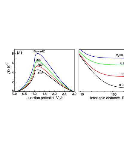
Figure 4: RKKY range function between two local spins mirror symmetric about the PNJ with $E_{F}=0$. (a) $\mathcal{J}$ vs. junction potential for different inter-spin distances $R$. (b) $\mathcal{J}R/a$ vs. $R$ for different junction potentials.

Let us consider the RKKY interaction between two mirror symmetric spins in graphene PNJ at $E_{F}=0$, i.e., electron doping $V_{0}$ in the N region and hole doping $V_{0}$ in the P region. According to the symmetry analysis in Sec. IIB, for the PNJ with its interface along the zigzag direction, the RKKY interaction between two mirror symmetric spins is always antiferromagnetic. This feature is demonstrated by Fig. 4. As shown in Fig. 4(a), in the linear regime ($V_{0}\ll t$), the RKKY interaction $\mathcal{J}\propto V_{0}^{2}$ increases quadratically with $V_{0}$. As shown in Fig. 4(b), the scaled RKKY interaction strength $\mathcal{J}R/a$ is $R$-independent at large distances. This indicates that $\mathcal{J}$ follows $1/R$ asymptotic decay due to the perfect refocusing, in sharp contrast to the $1/R^{d}$ asymptotic decay in a great diversity of doped $d$-dimensional materials, as well as the $1/R^{3}$ asymptotic decay in undoped graphene. Therefore, the RKKY interaction at $V_{0}\ll t$ and $R\gg\lambda_{F}$ can be well approximated by the analytical expression $\mathcal{J}\approx 0.012{(V_{0}/t)^{2}}/({R/a}),$ where the constant $0.012$ is obtained by fitting the data in Fig. 4(a)-(b). For comparison, in uniform graphene with the same doping level as the PNJ, the envelope of the RKKY interaction [see Eq. (8)] has the asymptotic form $\mathcal{J}_{\mathrm{uniform}}\approx 0.037({V_{0}/t})/({R^{2}/a^{2}})$. The RKKY interaction in the graphene PNJ differs qualitatively from that in uniform graphene in the scaling with both the distance ($\mathcal{J}_{\mathrm{uniform}}\propto 1/R^{2}$ vs. $\mathcal{J}\propto 1/R$) and the junction potential $V_{0}$ or equivalently carrier concentration ($\mathcal{J}_{\mathrm{uniform}}\propto V_{0}$ vs. $\mathcal{J}\propto V_{0}^{2}$). Since the localized spins are usually fixed, dynamic tuning of the PNJ by electric gating potentially allows for selective control of localized spins, an important ingredient for spin-based quantum computation.

III.2 Experimental feasibility and generalization to other materials

Since the focusing of the RKKY interaction is dominated by the contribution from the electron states near the Fermi level, and these states cannot not “feel” any potential variation on the length scale $\ll$ Fermi wavelength $\lambda_{F}$, the finite width of the PNJ has a small influence as long as it is much smaller than $\lambda_{F}$. Taking $V_{0}=0.1t$ and the first local spin at $\mathbf{R}_{1}=(-151a,0)$ as an example, using the experimentally fabricated linear PNJ Williams et al. (2011) of width $29a\approx 4.1$ nm, instead of a sharp PNJ, only reduces the magnitude of the RKKY interaction by $\sim 25\%$ without changing the $1/R$ asymptotic scaling.

In the presence of a finite gap $\Delta$ (e.g., due to substrate mismatch Hunt et al. (2013)) in the Dirac spectrum of graphene, as long as $\Delta\ll|V_{0}|$, the gap does not significantly influence the states near the Fermi level, which dominates the anomalous focusing effect. This has been confirmed by our numerical calculation using $E_{F}=0$, $V_{0}=0.2t$, and a typical gap $\Delta=0.03t$: no appreciable change of the focusing behavior occurs. As a matter of fact, from our analytical analysis following Eq. (6), it is clear that perfect focusing of the PNJ with $E_{F}=0$ essentially arises from the opposite momenta $q_{N,x}=-q_{P,x}=[(V_{0}/v_{F})^{2}-q_{y}^{2}]^{1/2}$ in the N region and P region of the PNJ, which suppresses the rapidly oscillating phase $\mathbf{q}_{P}\cdot\mathbf{R}_{2}-\mathbf{q}_{N}\cdot\mathbf{R}_{1}=0$ [see Eq. (6)] as long as $\mathbf{R}_{1}$ and $\mathbf{R}_{2}$ are mirror symmetric about the PNJ. The key ingredients of this effect are the circular Fermi contours and the opposite group velocities in the N region and P region, although the linear dispersion and gapless feature of graphene allows high transmission of electron waves (i.e., Klein tunneling) and hence quantitatively stronger focusing effect. Consequently, similar principle should lead to similar effect in other materials with a nonlinear dispersion and/or a finite gap (e.g., silicene PNJ Yamakage et al. (2013)). For example, we have numerically verified that the local enhancement of the RKKY interaction remains effective even when the gap of the graphene PNJ increases to $\Delta=0.1$ $t$.

The anomalous focusing is pronounced at low temperature and persists up to nitrogen temperature Cheianov et al. (2007). To observe the $1/R$ long-range RKKY interaction across the graphene PNJ, experiments should be carried out at a temperature higher than the Kondo temperature to avoid the screening of the local spins by the carriers Uchoa et al. (2011). The anomalous focusing in graphene PNJ has been demonstrated by two recent experiments Lee et al. (2015); Chen et al. (2016). Thus we expect our theoretical results to be experimentally accessible.

IV Summary

As opposed to previous works that explore the influence of electronic states and energy band structures of uniform 2D systems on the carrier-mediated RKKY interaction, we have proposed a very different way to manipulate the RKKY interaction: tailoring the carrier propagation and interference via a well-known electron optics phenomenon in graphene P-N junctions – the anomalous focusing effect. This gives rise to rich spatial interference patterns and locally enhanced, symmetry-protected non-oscillatory RKKY interaction, which may pave the way towards long-range spin-spin interaction for scalable graphene-based spintronics devices. The key physics leading to the focusing of the RKKY interaction is the focusing of the carrier spin fluctuation emanating from a local spin. In this context, we notice a very relevant work by Guimaraes et al. Guimaraes et al. (2011), which shows that a gate-defined curved boundary in graphene can focus the spin current emanating from a precessing magnetic moment onto a specific point. We expect that this spin current lens could be utilized as an alternative way to focus the RKKY interaction.

Appendix A Propagator in $\mathbf{K}$-valley continuum model

Here we derive the 2$\times$2 matrix propagator $\mathbf{g}(\mathbf{r},\mathbf{r}^{\prime},E)$ with $E\in[-V_{0},V_{0}]$ in the $\mathbf{K}$-valley continuum model [Eq. (4) of the main text]. Due to translational invariance along the $y$ axis, the 2D propagator

$$\mathbf{g}(\mathbf{r},\mathbf{r}^{\prime},E)\equiv\int\frac{dq_{y}}{2\pi}e^{iq_{y}(y-y^{\prime})}\mathbf{g}_{\mathrm{1D}}(x,x^{\prime},E)$$ (9)

is determined by the 1D propagator $\mathbf{g}_{\mathrm{1D}}(x,x^{\prime},E)$ of the 2$\times$2 Hamiltonian $\mathbf{h}_{\mathrm{1D}}(x,-i\partial_{x})=-iv_{F}\hat{\sigma}_{x}\partial_{x}+v_{F}\hat{\sigma}_{y}q_{y}+\mathrm{sgn}(x)V_{0}$, with the dependence of $\mathbf{g}_{\mathrm{1D}}(\cdots)$ and $\mathbf{h}_{\mathrm{1D}}(\cdots)$ on $q_{y}$ omitted for brevity. Here $\mathbf{g}_{\mathrm{1D}}(x,x^{\prime},E)$ obeys the differential equations

$$[E+i0^{+}-\mathbf{h}_{\mathrm{1D}}(x,-i\partial_{x})]\mathbf{g}_{\mathrm{1D}}(x,x^{\prime},E) =\delta(x-x^{\prime}),$$

$$\mathbf{g}_{\mathrm{1D}}(x,x^{\prime},E)[E+i0^{+}-\mathbf{h}_{\mathrm{1D}}(x^{\prime},-i\overleftarrow{\partial_{x^{\prime}}})] =\delta(x-x^{\prime}),$$

($\overleftarrow{\partial_{x^{\prime}}}$ acting on the left) and the continuity conditions

$$\mathbf{g}_{\mathrm{1D}}(x+0^{+},x,E)-\mathbf{g}_{\mathrm{1D}}(x-0^{+},x,E) =-i\sigma_{x}/v_{F},$$

$$\mathbf{g}_{\mathrm{1D}}(x,x+0^{+},E)-\mathbf{g}_{\mathrm{1D}}(x,x-0^{+},E) =i\sigma_{x}/v_{F}.$$

Then $\mathbf{g}_{\mathrm{1D}}(x,x^{\prime},E)$ is obtain by first calculating the general solutions in the region $x\neq x^{\prime}$ and then matching them using the boundary conditions.

To present the results in a physically intuitive way, we introduce the following concepts. Given the energy $E$ and momentum $q_{y}$, there is one right-going eigenstate $|+,\mathbf{q}_{N}\rangle$ with $\mathbf{q}_{N}\equiv(q_{N,x},q_{y})$ and one left-going eigenstate $|+,\mathbf{\tilde{q}}_{N}\rangle$ with $\mathbf{\tilde{q}}_{N}\equiv(-q_{N,x},q_{y})$ in the N region, as well as one right-going eigenstate $|-,\mathbf{q}_{P}\rangle$ with $\mathbf{q}_{P}\equiv(q_{P,x},q_{y})$ and one left-going eigenstate $|-,\mathbf{\tilde{q}}_{P}\rangle$ with $\mathbf{\tilde{q}}_{P}\equiv(-{q}_{P,x},q_{y})$ in the P region, where $|s,\mathbf{q}\rangle\propto e^{i\mathbf{q}\cdot\mathbf{r}}|u_{s}(\mathbf{q})\rangle$ is the eigenstate of uniform graphene in the conduction band $(s=+)$ or valence band $(s=-$). For small $|q_{y}|$, we choose $q_{N,x}>0$ and $q_{P,x}<0$, so that $|+,\mathbf{q}_{N}\rangle$ and $|-,\mathbf{q}_{P}\rangle$ ($|+,\mathbf{\tilde{q}}_{N}\rangle$ and $|-,\mathbf{\tilde{q}}_{P}\rangle$) propagate from the left (right) to the right (left) without decay. For large $|q_{y}|$, we choose $\operatorname{Im}q_{N,x}>0$ and $\operatorname{Im}q_{P,x}>0$, so that $|+,\mathbf{q}_{N}\rangle$ and $|-,\mathbf{q}_{P}\rangle$ ($|+,\mathbf{\tilde{q}}_{N}\rangle$ and $|-,\mathbf{\tilde{q}}_{P}\rangle$) decays to zero at $x\rightarrow+\infty$ $(x\rightarrow-\infty)$.

In terms of these left-going and right-going eigenstates with given energy $E$ and $q_{y}$, the 1D propagator from $x^{\prime}$ in the N region to $x$ in the P region is

$$\mathbf{g}_{\mathrm{1D}}(x,x^{\prime},E)=\frac{w(q_{y})}{iv_{x}(\mathbf{q}_{N})}|u_{-}(\mathbf{q}_{P})\rangle\langle u_{+}(\mathbf{q}_{N})|e^{i(q_{P,x}x-q_{N,x}x^{\prime})},$$ (10)

where $w(q_{y})=2\cos\theta_{N}/(e^{-i\theta_{N}}+e^{i\theta_{P}})$ is the transmission coefficient and $\mathbf{v}(\mathbf{q})\equiv v_{F}\mathbf{q}/|\mathbf{q}|$ is the group velocity, with $\theta_{N}$ ($\theta_{P}$) is the incident (transmission) angle defined via $v_{F}(q_{N,x}+iq_{y})=(E+V_{0})e^{i\theta_{N}}$ and $v_{{}_{F}}(q_{P,x}+iq_{y})=-(V_{0}-E)e^{i\theta_{P}}$. Substituting Eq. (10) into Eq. (9) gives the 2D propagator $\mathbf{g}(\mathbf{r},\mathbf{r}^{\prime},E)|_{\mathbf{r}^{\prime}\in\mathrm{N},\mathbf{r}\in\mathrm{P}}$ in Eq. (6) of the main text. For $x^{\prime}<x<0$, the 2D propagator $\mathbf{g}(\mathbf{r},\mathbf{r}^{\prime},E)$ is the sum of the direct, forward propagation from $\mathbf{r}^{\prime}$ to $\mathbf{r}$,

$$\int\frac{dq_{y}}{2\pi}\frac{|u_{+}(\mathbf{q}_{N})\rangle\langle u_{+}(\mathbf{q}_{N})|}{iv_{x}(\mathbf{q}_{N})}e^{i\mathbf{q}_{N}\cdot(\mathbf{r}-\mathbf{r}^{\prime})},$$

and the contribution from the reflected wave

$$\int\frac{dq_{y}}{2\pi}r(q_{y})\frac{|u_{+}(\mathbf{\tilde{q}}_{N})\rangle\langle u_{+}(\mathbf{q}_{N})|}{iv_{x}(\mathbf{q}_{N})}e^{i\mathbf{\tilde{q}}_{N}\cdot\mathbf{r}}e^{-i\mathbf{q}_{N}\cdot\mathbf{r}^{\prime}}$$

via three steps: the propagation from $\mathbf{r}^{\prime}$ to the PNJ, the reflection by the PNJ, and the propagation of the reflected wave from the PNJ to $\mathbf{r}$. For $x<x^{\prime}<0$, $\mathbf{g}(\mathbf{r},\mathbf{r}^{\prime},E)$ is obtained from $\mathbf{g}(\mathbf{r},\mathbf{r}^{\prime},E)|_{x^{\prime}<x<0}$ by replacing the direct, forward propagation by the direct, backward propagation:

$$\int\frac{dq_{y}}{2\pi}\frac{|u_{+}(\mathbf{\tilde{q}}_{N})\rangle\langle u_{+}(\mathbf{\tilde{q}}_{N})|}{iv_{x}(\mathbf{q}_{N})}e^{i\mathbf{\tilde{q}}_{N}\cdot(\mathbf{r}-\mathbf{r}^{\prime})}.$$

Appendix B Symmetry of propagators and RKKY interaction in tight-binding model

In the tight-binding model, the propagator from $\mathbf{R}^{\prime}$ to $\mathbf{R}$ is $G(\mathbf{R},\mathbf{R}^{\prime},E)\equiv\langle\mathbf{R}|(E-\hat{H}+i0^{+})^{-1}|\mathbf{R}^{\prime}\rangle$. Using the invariance $\hat{\theta}\hat{H}\hat{\theta}^{-1}=\hat{H}$ and $\hat{\theta}|\mathbf{R}\rangle=|\mathbf{R}\rangle$ under time-reversal transformation, we have $G(\mathbf{R},\mathbf{R}^{\prime},E)\equiv\langle\mathbf{R}|(E-\hat{H}-i0^{+})^{-1}|\mathbf{R}^{\prime}\rangle^{\ast}=G(\mathbf{R}^{\prime},\mathbf{R},E)$. Inverting the nearest-neighbor hopping amplitude $t\rightarrow-t$ amounts to the transformation $|\mathbf{R}\rangle\rightarrow\mathrm{sgn}(\mathbf{R})|\mathbf{R}\rangle$ in the Hamiltonian and hence $G(\mathbf{R},\mathbf{R}^{\prime},E)|_{t\rightarrow-t}=\mathrm{sgn}(\mathbf{R})\mathrm{sgn}(\mathbf{R}^{\prime})G(\mathbf{R},\mathbf{R}^{\prime},E)$, where $\mathrm{sgn}(\mathbf{R})=+1$ if $\mathbf{R}$ locates on the $A$ sublattice and $\mathrm{sgn}(\mathbf{R})=-1$ if $\mathbf{R}$ locates on the $B$ sublattice. Since $\hat{H}\rightarrow-\hat{H}$ under $(V_{0},t)\rightarrow(-V_{0},-t)$ and $\hat{\theta}\hat{H}\hat{\theta}^{-1}=\hat{H}$, we have

$$G(\mathbf{R},\mathbf{R}^{\prime},E) \rightarrow-\langle\mathbf{R}|(E-\hat{H}-i0^{+})^{-1}|\mathbf{R}^{\prime}\rangle$$

$$=-\langle\mathbf{R}|(E-\hat{H}+i0^{+})^{-1}|\mathbf{R}^{\prime}\rangle^{\ast}$$

$$=-G^{\ast}(\mathbf{R},\mathbf{R}^{\prime},E)$$

under $(E,V_{0},t)\rightarrow(-E,-V_{0},-t)$. Combining the transformation properties of the propagator under $t\rightarrow-t$ and $(E,V_{0},t)\rightarrow(-E,-V_{0},-t)$ gives $G(\mathbf{R},\mathbf{R}^{\prime},E)\rightarrow-\mathrm{sgn}(\mathbf{R})\mathrm{sgn}(\mathbf{R}^{\prime})G^{\ast}(\mathbf{R},\mathbf{R}^{\prime},E)$ upon $(E,V_{0})\rightarrow(-E,-V_{0})$. Using the generalized electron-hole symmetry of the graphene PNJ, we also have $G(\mathbf{R},\mathbf{R}^{\mathrm{m}},E)=-\mathrm{sgn}(\mathbf{R})\mathrm{sgn}(\mathbf{R}^{\mathrm{m}})G^{\ast}(\mathbf{R},\mathbf{R}^{\mathrm{m}},-E)$.

The above transformation properties of the propagator leads to the corresponding properties of the RKKY range function $J$, e.g., $J$ is invariant upon $t\rightarrow-t$. Similarly, upon $(V_{0},E_{F})\rightarrow(-V_{0},-E_{F})$, we have

$$J \rightarrow-\frac{J_{0}^{2}}{2\pi}\int_{E_{F}}^{+\infty}dE\operatorname{Im}G^{2}({\mathbf{R}_{2}},{\mathbf{R}_{1}},-E)|_{V_{0}\rightarrow-V_{0}}$$

$$=\frac{J_{0}^{2}}{2\pi}\int_{E_{F}}^{+\infty}dE\operatorname{Im}G^{2}({\mathbf{R}_{2}},{\mathbf{R}_{1}},E).$$

Using $\int_{-\infty}^{\infty}\operatorname{Im}G^{2}({\mathbf{R}_{2}},{\mathbf{R}_{1}},E)dE=0$, we see that $J$ is invariant upon $(V_{0},E_{F})\rightarrow(-V_{0},-E_{F})$. Also, when the two spins locate at mirror symmetric points $\mathbf{R}$ and $\mathbf{R}^{\mathrm{m}}$, their RKKY interaction $J$ is invariant upon $E_{F}\rightarrow-E_{F}$.

References

- Castro Neto et al. (2009) A. H. Castro Neto, F. Guinea, N. M. R. Peres, K. S. Novoselov, and A. K. Geim, Rev. Mod. Phys. 81, 109 (2009).
- Cheianov et al. (2007) V. V. Cheianov, V. Fal’ko, and B. L. Altshuler, Science 315, 1252 (2007).
- Veselago (1968) V. G. Veselago, Soviet Physics Uspekhi 10, 509 (1968).
- Pendry (2000) J. B. Pendry, Phys. Rev. Lett. 85, 3966 (2000).
- Zhang and Liu (2008) X. Zhang and Z. Liu, Nat. Mater. 7, 435 (2008).
- Pendry et al. (2012) J. B. Pendry, A. Aubry, D. R. Smith, and S. A. Maier, Science 337, 549 (2012).
- Cserti et al. (2007) J. Cserti, A. Pályi, and C. Péterfalvi, Phys. Rev. Lett. 99, 246801 (2007).
- Garcia-Pomar et al. (2008) J. L. Garcia-Pomar, A. Cortijo, and M. Nieto-Vesperinas, Phys. Rev. Lett. 100, 236801 (2008).
- Moghaddam and Zareyan (2010) A. G. Moghaddam and M. Zareyan, Phys. Rev. Lett. 105, 146803 (2010).
- Silveirinha and Engheta (2013) M. G. Silveirinha and N. Engheta, Phys. Rev. Lett. 110, 213902 (2013).
- Zhao et al. (2013) L. Zhao, P. Tang, B.-L. Gu, and W. Duan, Phys. Rev. Lett. 111, 116601 (2013).
- Lee et al. (2015) G.-H. Lee, G.-H. Park, and H.-J. Lee, Nat. Phys. 11, 925 (2015).
- Chen et al. (2016) S. Chen, Z. Han, M. M. Elahi, K. M. M. Habib, L. Wang, B. Wen, Y. Gao, T. Taniguchi, K. Watanabe, J. Hone, et al., Science 353, 1522 (2016).
- Ruderman and Kittel (1954) M. A. Ruderman and C. Kittel, Phys. Rev. 96, 99 (1954).
- Kasuya (1956) T. Kasuya, Prog. Theor. Phys. 16, 45 (1956).
- Yosida (1957) K. Yosida, Phys. Rev. 106, 893 (1957).
- Wolf et al. (2001) S. A. Wolf, D. D. Awschalom, R. A. Buhrman, J. M. Daughton, S. von Molnar, M. L. Roukes, A. Y. Chtchelkanova, and D. M. Treger, Science 294, 1488 (2001).
- Zutic et al. (2004) I. Zutic, J. Fabian, and S. Das Sarma, Rev. Mod. Phys. 76, 323 (2004).
- MacDonald et al. (2005) A. H. MacDonald, P. Schiffer, and N. Samarth, Nat. Mater. 4, 195 (2005).
- Loss and DiVincenzo (1998) D. Loss and D. P. DiVincenzo, Phys. Rev. A 57, 120 (1998).
- Trifunovic et al. (2012) L. Trifunovic, O. Dial, M. Trif, J. R. Wootton, R. Abebe, A. Yacoby, and D. Loss, Phys. Rev. X 2, 011006 (2012).
- Klinovaja et al. (2013) J. Klinovaja, P. Stano, A. Yazdani, and D. Loss, Phys. Rev. Lett. 111, 186805 (2013).
- Piermarocchi et al. (2002) C. Piermarocchi, P. Chen, L. J. Sham, and D. G. Steel, Phys. Rev. Lett. 89, 167402 (2002).
- Craig et al. (2004) N. J. Craig, J. M. Taylor, E. A. Lester, C. M. Marcus, M. P. Hanson, and A. C. Gossard, Science 304, 565 (2004).
- Rikitake and Imamura (2005) Y. Rikitake and H. Imamura, Phys. Rev. B 72, 033308 (2005).
- Friesen et al. (2007) M. Friesen, A. Biswas, X. Hu, and D. Lidar, Phys. Rev. Lett. 98, 230503 (2007).
- Srinivasa et al. (2015) V. Srinivasa, H. Xu, and J. M. Taylor, Phys. Rev. Lett. 114, 226803 (2015).
- Fischer and Klein (1975) B. Fischer and M. W. Klein, Phys. Rev. B 11, 2025 (1975).
- Béal-Monod (1987) M. T. Béal-Monod, Phys. Rev. B 36, 8835 (1987).
- Brey et al. (2007) L. Brey, H. A. Fertig, and S. Das Sarma, Phys. Rev. Lett. 99, 116802 (2007).
- Saremi (2007) S. Saremi, Phys. Rev. B 76, 184430 (2007).
- Black-Schaffer (2010a) A. M. Black-Schaffer, Phys. Rev. B 81, 205416 (2010a).
- Sherafati and Satpathy (2011a) M. Sherafati and S. Satpathy, Phys. Rev. B 83, 165425 (2011a).
- Sherafati and Satpathy (2011b) M. Sherafati and S. Satpathy, Phys. Rev. B 84, 125416 (2011b).
- Uchoa et al. (2011) B. Uchoa, T. G. Rappoport, and A. H. Castro Neto, Phys. Rev. Lett. 106, 016801 (2011).
- Kogan (2011) E. Kogan, Phys. Rev. B 84, 115119 (2011).
- Liu et al. (2009) Q. Liu, C.-X. Liu, C. Xu, X.-L. Qi, and S.-C. Zhang, Phys. Rev. Lett. 102, 156603 (2009).
- Zhu et al. (2011) J.-J. Zhu, D.-X. Yao, S.-C. Zhang, and K. Chang, Phys. Rev. Lett. 106, 097201 (2011).
- Abanin and Pesin (2011) D. A. Abanin and D. A. Pesin, Phys. Rev. Lett. 106, 136802 (2011).
- Inosov et al. (2009) D. S. Inosov, D. V. Evtushinsky, A. Koitzsch, V. B. Zabolotnyy, S. V. Borisenko, A. A. Kordyuk, M. Frontzek, M. Loewenhaupt, W. Löser, I. Mazilu, et al., Phys. Rev. Lett. 102, 046401 (2009).
- Zhu et al. (2010) J.-J. Zhu, K. Chang, R.-B. Liu, and H.-Q. Lin, Phys. Rev. B 81, 113302 (2010).
- Néel et al. (2011) N. Néel, R. Berndt, J. Kröger, T. O. Wehling, A. I. Lichtenstein, and M. I. Katsnelson, Phys. Rev. Lett. 107, 106804 (2011).
- Yao et al. (2014) N. Y. Yao, L. I. Glazman, E. A. Demler, M. D. Lukin, and J. D. Sau, Phys. Rev. Lett. 113, 087202 (2014).
- Holub et al. (2004) M. Holub, S. Chakrabarti, S. Fathpour, P. Bhattacharya, Y. Lei, and S. Ghosh, Appl. Phys. Lett. 85, 973 (2004).
- Xiu et al. (2010) F. Xiu, Y. Wang, J. Kim, A. Hong, J. Tang, A. P. Jacob, J. Zou, and K. L. Wang, Nat. Mater. 9, 337 (2010).
- Nie et al. (2016) T. Nie, J. Tang, X. Kou, Y. Gen, S. Lee, X. Zhu, Q. He, L.-T. Chang, K. Murata, Y. Fan, et al., Nat. Commun. 7, 12866 (2016).
- Bouhassoune et al. (2014) M. Bouhassoune, B. Zimmermann, P. Mavropoulos, D. Wortmann, P. H. Dederichs, S. Blügel, and S. Lounis, Nat. Commun. 5, 5558 (2014).
- Power et al. (2012) S. R. Power, P. D. Gorman, J. M. Duffy, and M. S. Ferreira, Phys. Rev. B 86, 195423 (2012).
- Meier et al. (2008) F. Meier, L. Zhou, J. Wiebe, and R. Wiesendanger, Science 320, 82 (2008).
- Zhou et al. (2010) L. Zhou, J. Wiebe, S. Lounis, E. Vedmedenko, F. Meier, S. Blugel, P. H. Dederichs, and R. Wiesendanger, Nat. Phys. 6, 187 (2010).
- Khajetoorians et al. (2012) A. A. Khajetoorians, J. Wiebe, B. Chilian, S. Lounis, S. Blugel, and R. Wiesendanger, Nat. Phys. 8, 497 (2012).
- Klier et al. (2015) N. Klier, S. Shallcross, S. Sharma, and O. Pankratov, Phys. Rev. B 92, 205414 (2015).
- Black-Schaffer (2010b) A. M. Black-Schaffer, Phys. Rev. B 82, 073409 (2010b).
- Bruno (1995) P. Bruno, Phys. Rev. B 52, 411 (1995).
- Zhang et al. (2016) S.-H. Zhang, J.-J. Zhu, W. Yang, H.-Q. Lin, and K. Chang, Phys. Rev. B 94, 085408 (2016).
- Katsnelson et al. (2006) M. I. Katsnelson, K. S. Novoselov, and A. K. Geim, Nat. Phys. 2, 620 (2006).
- Logemann et al. (2015) R. Logemann, K. J. A. Reijnders, T. Tudorovskiy, M. I. Katsnelson, and S. Yuan, Phys. Rev. B 91, 045420 (2015).
- Bunder and Lin (2009) J. E. Bunder and H.-H. Lin, Phys. Rev. B 80, 153414 (2009).
- Mahan (2000) G. D. Mahan, Many-Particle Physics (Kluwer Academic/Plenum Publishers, New York, 2000).
- Lee et al. (2012) H. Lee, E. Mucciolo, G. Bouzerar, and S. Kettemann, Phys. Rev. B 86, 205427 (2012).
- Williams et al. (2011) J. R. Williams, T. Low, M. S. Lundstrom, and C. M. Marcus, Nat Nano 6, 222 (2011).
- Hunt et al. (2013) B. Hunt, J. D. Sanchez-Yamagishi, A. F. Young, M. Yankowitz, B. J. LeRoy, K. Watanabe, T. Taniguchi, P. Moon, M. Koshino, P. Jarillo-Herrero, et al., Science 340, 1427 (2013).
- Yamakage et al. (2013) A. Yamakage, M. Ezawa, Y. Tanaka, and N. Nagaosa, Phys. Rev. B 88, 085322 (2013).
- Guimaraes et al. (2011) F. S. M. Guimaraes, A. T. Costa, R. B. Muniz, and M. S. Ferreira, Journal of Physics: Condensed Matter 23, 175302 (2011).