Impact of Line-of-Sight and Unequal Spatial Correlation on Uplink MU-MIMO Systems

Abstract

Closed-form approximations of the expected per-terminal signal-to-interference-plus-noise-ratio (SINR) and ergodic sum spectral efficiency of a multiuser multiple-input multiple-output system are presented. Our analysis assumes spatially correlated Ricean fading channels with maximum-ratio combining on the uplink. Unlike previous studies, our model accounts for the presence of unequal correlation matrices, unequal Rice factors, as well as unequal link gains to each terminal. The derived approximations lend themselves to useful insights, special cases and demonstrate the aggregate impact of line-of-sight (LoS) and unequal correlation matrices. Numerical results show that while unequal correlation matrices enhance the expected SINR and ergodic sum spectral efficiency, the presence of strong LoS has an opposite effect. Our approximations are general and remain insensitive to changes in the system dimensions, signal-to-noise-ratios, LoS levels and unequal correlation levels.

I Introduction

The lack of rich scattering and insufficient antenna spacing at a cellular base station (BS) leads to increased levels of spatial correlation [1]. For multiuser multiple-input multiple-output (MU-MIMO) systems, this is known to negatively impact the signal-to-interference-plus-noise-ratio (SINR) of a given terminal, as well as the sum spectral efficiency of the system. Numerous works have investigated the SINR and spectral efficiency performance of MU-MIMO systems with spatial correlation (see e.g., [2, 3, 4] and references therein). However, very few of the above mentioned studies consider the effects of line-of-sight (LoS) components, likely to be a dominant feature in future wireless access with the rise of smaller cell sizes [5]. Thus, understanding the performance of such systems with Ricean fading is of particular importance. The uplink Ricean analysis presented in [6] does not consider the effects of spatial correlation at the BS. On the other hand, the related literature (see e.g., [7, 3]) routinely assumes that on the uplink, all terminals are seen by the BS via the same set of incident directions, resulting in equal correlation structures. In reality, a different set of incident directions are likely to be observed by multiple terminals, due to their different geographical locations, leading to variations in the local scattering. This gives rise to wide variations in the correlation patterns across multiple terminals [4]. Hence, we consider unequal correlation matrices from each terminal.

Motivated by this, with a uniform linear array (ULA) and maximum-ratio combining (MRC) at the BS, we present insightful closed-form approximations of the expected perterminal SINR and ergodic sum spectral efficiency of an uplink MU-MIMO system. Unlike previous results, for both microwave and millimeter-wave (mmWave) propagation parameters, the closed-form expressions consider unequal correlation matrices, Rice ($K$) factors and link gains for each terminal. The approximations are shown to be extremely tight for small and large system dimensions, as well as, arbitrary signal-to-noise- ratios (SNRs). To the best of our knowledge, this level of accuracy over such a general channel model capturing a wide range of scenarios has not been achieved previously. Numerical results show the aggregate impact of LoS and unequal spatial correlation. Special cases are presented for Rayleigh fading channels with equal and unequal correlation matrices, as well as, for Ricean fading channels with equal correlation matrices.

II System Model

The uplink of a MU-MIMO system operating in an urban microcellular environment (UMi) is considered. The BS is located at the center of a circular cell with radius $R_{c}$, and is equipped with a $M$ element ULA simultaneously communicating with $L$ single-antenna terminals ($M\gg{}L$). Channel knowledge is assumed at the BS, as the prime focus of the manuscript is on performance analysis with general fading channels and not on system level imperfections.

The composite $M\times{}1$ received signal at the BS is given by $\bm{y}=\rho^{\frac{1}{2}}\bm{G}\bm{D}^{\frac{1}{2}}\bm{s}+\bm{n}$, where $\rho$ is the average uplink transmit power, $\bm{G}$ is the $M\times{}L$ fast-fading channel matrix between the $M$ BS antennas and $L$ terminals, $\bm{D}$ is an $L\times{}L$ diagonal matrix of link gains, where the link gain for terminal $l$ is given by $\left[\bm{D}\right]_{l,l}=\beta_{l}$. The large-scale fading effects for terminal $l$ in geometric attenuation and shadow-fading are captured in $\beta_{l}=\varrho{}\zeta_{l}\left(r_{0}/r_{l}\right)^{\alpha}$. In particular, $\varrho$ is the unit-less constant for geometric attenuation at a reference distance of $r_{0}$, $r_{l}$ is the distance between the $l$-th terminal and the BS, $\alpha$ is the attenuation exponent and $\zeta_{l}$ captures the effects of shadow-fading, modeled via a log-normal density, i.e., $10\log_{10}\left(\zeta_{l}\right)\sim{}\mathcal{N}\left(0,\sigma_{\textrm{sh}}^{2}\right)$. Moreover, $\bm{s}$ is the $L\times{}1$ vector of uplink data symbols from $L$ terminals to the BS, such that the $l$-th entry of $\bm{s}$, $s_{l}$ has an expected value of one, i.e., $\mathbb{E}\left[|s_{l}|^{2}\right]=1$. The $M\times{}1$ vector of additive white Gaussian noise at the BS is denoted by $\bm{n}$, such that the $l$-th entry of $\bm{n}$, $n_{l}\sim{}\mathcal{CN}\left(0,\sigma^{2}\right)$. We assume that $\sigma^{2}=1$. Hence, the average uplink SNR is defined as $\rho/\sigma^{2}=\rho$. The $M\times{}1$ channel vector from terminal $l$ to the BS is denoted by $\bm{g}_{l}$, which forms the $l$-th column of $\bm{G}=\left[\bm{g}_{1},\dots,\bm{g}_{L}\right]$.

More specifically,

$$\bm{g}_{l}=\eta_{l}\bar{\bm{h}}_{l}+\gamma_{l}\bm{R}_{l}^{\frac{1}{2}}\tilde{\bm{h}}_{l}.\vspace{-5pt}$$ (1)

The $M\times{}1$ LoS and the non LoS (NLoS) components of the channel are denoted by $\bar{\bm{h}}_{l}$ and $\tilde{\bm{h}}_{l}$. Note that $\gamma_{l}=(1/\left(1+K_{l}\right))^{1/2}$ and $\eta_{l}=(K_{l}/\left(K_{l}+1\right))^{1/2}$, with $K_{l}$ being the Ricean $K$-factor for the $l$-th terminal. $\bm{R}_{l}$ is the receive correlation matrix specific to terminal $l$, $\tilde{\bm{h}}_{l}\sim\mathcal{CN}\left(0,\bm{I}_{M}\right)$ and $\bar{\bm{h}}_{l}=[1,e^{j2\pi{}d\cos\left(\phi^{\prime}_{l}\right)},\dots,e^{j2\pi{}d\left(M-1\right)\cos\left(\phi^{\prime}_{l}\right)}]$. Here, $d$ is the equidistant inter-element antenna spacing normalized by the carrier wavelength and $\phi^{\prime}_{l}\sim{}\mathcal{U}\left[0,2\pi\right]$ is the azimuth angle-of-arrival of the LoS component for the $l$-th terminal.

We employ a linear receiver at the BS array in the form of a MRC filter, where $\bm{G}^{\textrm{H}}$ is the $L\times{}M$ filter matrix used to separate $\bm{y}$ into $L$ data streams by $\bm{r}=\bm{G}^{\textrm{H}}\bm{y}=\rho^{1/2}\bm{G}^{\textrm{H}}\bm{G}\bm{D}^{1/2}\bm{s}+\bm{G}^{\textrm{H}}\bm{n}$. Hence, the combined signal from terminal $l$ is given by $r_{l}=\rho^{1/2}\beta_{l}^{1/2}\bm{g}_{l}^{\textrm{H}}\bm{g}_{l}s_{l}+\rho^{1/2}\sum\nolimits_{\begin{subarray}{c}k=1\\ k\neq{}l\end{subarray}}^{L}\beta_{k}^{1/2}\bm{g}_{l}^{\textrm{H}}\bm{g}_{k}s_{k}+\bm{g}_{l}^{\textrm{H}}\bm{n}$. Thus, the corresponding SINR for terminal $l$ is given by

$$\textrm{SINR}_{l}=\frac{\rho\beta_{l}||\bm{g}_{l}||^{4}}{||\bm{g}_{l}||^{2}+\rho\sum\nolimits_{\begin{subarray}{c}k=1\\ k\neq{}l\end{subarray}}^{L}\beta_{k}|\bm{g}_{l}^{\textrm{H}}\bm{g}_{k}|^{2}}.\vspace{-5pt}$$ (2)

As such, the instantaneous uplink spectral efficiency for the $l$-th terminal (measurable in bits/sec/Hz) is given by $\textrm{R}_{l}^{\textrm{se}}=\log_{2}\left(1+\textrm{SINR}_{l}\right)$. From here, the ergodic sum spectral efficiency over all $L$ terminals is given by

$$\mathbb{E}\left[\textrm{R}^{\textrm{sum}}\right]=\mathbb{E}\left[\sum\nolimits_{l=1}^{L}\textrm{R}_{l}^{\textrm{se}}\right],\vspace{-4pt}$$ (3)

where the expectation is performed over the fast-fading.

III Expected Per-Terminal SINR and Ergodic Sum Spectral Efficiency Analysis

The expected SINR of terminal $l$ can be obtained by evaluating the expected value of the ratio in (2). Exact evaluation of this is extremely cumbersome, as shown in [6]. Hence, we resort to the first-order Delta method expansion, as shown in the analysis methodology of [6]. This gives

$$\mathbb{E}\left[\textrm{SINR}_{l}\right]\approx\frac{\rho\beta_{l}\mathbb{E}\left[||\bm{g}_{l}||^{4}\right]}{\mathbb{E}\left[||\bm{g}_{l}||\right]^{2}+\rho\sum\nolimits_{\begin{subarray}{c}k=1\\ k\neq{}l\end{subarray}}^{L}\beta_{k}\mathbb{E}\left[|\bm{g}_{l}^{\textrm{H}}\bm{g}_{k}|^{2}\right]}.\vspace{-8pt}$$ (4)

Remark 1. The approximation in (4) is of the form of $\frac{\mathbb{E}\left[X\right]}{\mathbb{E}\left[Y\right]}$. The accuracy of such an approximation relies on $Y$ having a small standard deviation relative to its mean. This can be seen by applying a multivariate Taylor series expansion of $\frac{X}{Y}$ around $\frac{\mathbb{E}\left[X\right]}{\mathbb{E}\left[Y\right]}$, as shown in the methodology of [6]. Both $X$ and $Y$ are well suited to this approximation as $M$ and $L$ start to increase. This is evident from the presented numerical results in Section V.

In Lemmas 1, 2 and 3 which follow, we derive the expected values in the numerator and denominator of (4).

Lemma 1. For a ULA with $M$ receive antennas at the BS, considering a correlated Ricean fading channel, $\bm{g}_{l}$, from the $l$-th terminal to the BS

$$\delta_{l} =\mathbb{E}\left[||\bm{g}_{l}||^{4}\right]=\left(\eta_{l}\right)^{4}\left\{M^{2}+\textrm{tr}\left[\left(\bm{R}_{l}\right)^{2}\right]\right\}+2M^{2}\left(\eta_{l}\right)^{2}\left(\gamma_{l}\right)^{2}$$

$$+2\left(\gamma_{l}\right)^{2}\left(\eta_{l}\right)^{2}\left[\bar{\bm{h}}_{l}^{\textrm{H}}\bm{R}_{l}\bar{\bm{h}}_{l}\right]+\left(\gamma_{l}\right)^{4}M^{2},$$ (5)

where each parameter is defined after (1).

Proof: See Appendix A. ∎

Lemma 2. Under the same conditions as Lemma 1,

$$\varphi_{l,k} \hskip 2.0pt=\mathbb{E}\left[|\bm{g}_{l}^{\textrm{H}}\bm{g}_{k}|^{2}\right]=\left(\eta_{l}\right)^{2}\left(\eta_{k}\right)^{2}\textrm{tr}\left[\bm{R}_{k}\bm{R}_{l}\right]$$

$$+\left(\eta_{l}\right)^{2}\left(\gamma_{k}\right)^{2}\textrm{tr}\left[\bar{\bm{h}}_{k}^{\textrm{H}}\bm{R}_{l}\bar{\bm{h}}_{k}\right]+\left(\gamma_{l}\right)^{2}\left(\eta_{k}\right)^{2}\textrm{tr}\left[\bar{\bm{h}}_{l}\bar{\bm{h}}_{l}^{\textrm{H}}\bm{R}_{k}\right]$$

$$+\left(\gamma_{l}\right)^{2}\left(\gamma_{k}\right)^{2}|\bar{\bm{h}}_{l}^{\textrm{H}}\bar{\bm{h}}_{k}|^{2}.$$ (6)

Proof: See Appendix B. ∎

Lemma 3. Under the same conditions as Lemma 1,

$$\chi_{l}=\mathbb{E}\left[||\bm{g}_{l}||^{2}\right]=M\left[\left(\gamma_{l}\right)^{2}+\left(\eta_{l}\right)^{2}\right]=M.\vspace{-7pt}$$ (7)

Proof: We begin by recognizing that $\chi_{l}=\mathbb{E}\left[||\bm{g}_{l}||^{2}\right]=\mathbb{E}\big{[}\bm{g}_{l}^{\textrm{H}}\bm{g}_{l}\big{]}.$ Substituting the definition of $\bm{g}_{l}$ into (7) and performing the expectations in with respect to $\tilde{\bm{h}}$ yields the desired result. Only a sketch of the proof is given here, as it relies on straightforward algebraic manipulations.∎

Theorem 1. With MRC and a ULA at the BS, the expected uplink SINR of terminal $l$ undergoing spatially correlated Ricean fading can be approximated as

$$\mathbb{E}\left[\textrm{SINR}_{l}\right]\approx\frac{\rho\beta_{l}\delta_{l}}{\chi_{l}+\rho\sum\nolimits_{\begin{subarray}{c}k=1\\ k\neq{}l\end{subarray}}^{L}\beta_{k}\varphi_{l,k}},\vspace{-4pt}$$ (8)

where $\delta_{l},\varphi_{l,k}$ and $\chi_{l}$ are given by (5), (6) and (7), respectively.

Proof: Substituting the results from Lemmas 1, 2 and 3 for $\delta_{l},\chi_{l}$ and $\varphi_{l,k}$ yields the desired expression. ∎

Remark 2. Further algebraic manipulations allows us to express (8) as (10), shown on top of the next page for reasons of space. Note that (10) can be used to approximate the ergodic sum spectral efficiency of the system by stating

$$\mathbb{E}\left[\textrm{R}^{\textrm{sum}}\right]\approx\sum\nolimits_{l=1}^{L}\log_{2}\big{(}1+\mathbb{E}\left[\textrm{SINR}_{l}\right]\big{)}.\vspace{-4pt}$$ (9)

While the accuracy of (10) and (9) is demonstrated in Section V, in the sequel, we present the implications and special cases of (10) to demonstrate its generality.

IV Implications and Special Cases

IV-A Implications of (10)

$$\mathbb{E}\left[\textrm{SINR}_{l}\right]\approx\frac{\frac{\rho\beta_{l}}{\left(K_{l}+1\right)^{2}}\left\{M^{2}\left(1+2K_{l}+K_{l}^{2}\right)+\textrm{tr}\left[\bm{R}_{l}^{2}\right]+2K_{l}\bar{\bm{h}}_{l}^{\textrm{H}}\bm{R}_{l}\bar{\bm{h}}_{l}\right\}}{M+\rho\sum\nolimits_{k=1,k\neq{}l}^{L}\frac{\beta_{k}}{\left(K_{k}+1\right)\left(K_{l}+1\right)}\left\{\textrm{tr}\left[\bm{R}_{k}\bm{R}_{l}\right]+K_{k}\left(\bar{\bm{h}}_{k}^{\textrm{H}}\bm{R}_{l}\bar{\bm{h}}_{k}\right)+K_{l}\left(\bar{\bm{h}}_{l}^{\textrm{H}}\bm{R}_{k}\bar{\bm{h}}_{l}\right)+K_{l}K_{k}\left|\bar{\bm{h}}_{l}^{\textrm{H}}\bar{\bm{h}}_{k}\right|^{2}\right\}}.\vspace{-5pt}$$ (10)

Both the numerator and the denominator of (10) contain quadratic forms of the type $\bar{\bm{h}}^{\textrm{H}}\bm{R}\bar{\bm{h}}$. Via the Rayleigh quotient result, such quadratic forms are maximized when $\bar{\bm{h}}$ is parallel (aligned) to the maximum eigenvector of $\bm{R}$. From this, an interesting observation can be made: Alignment of $\bar{\bm{h}}_{l}$ and $\bm{R}_{l}$ amplifies the expected signal power, while alignment of $\bar{\bm{h}}_{k}$ with $\bm{R}_{l}$, $\bar{\bm{h}}_{l}$ with $\bm{R}_{k}$ and $\bar{\bm{h}}_{l}$ with $\bar{\bm{h}}_{k}$ increases the expected interference power, leading to a lower SINR. Likewise, if $\bm{R}_{k}$ and $\bm{R}_{l}$ become similar, then $\textrm{tr}\left[\bm{R}_{k}\bm{R}_{l}\right]$ increases, degrading the SINR. The global observation is that the SINR reduces by virtue of channel similarities of various types (LoS and correlation) and increases if the channels are more diverse.

IV-B Special Cases of (10)

Corollary 1. In pure NLoS conditions (i.e., Rayleigh fading) with unequal correlation matrices, (10) reduces to

$$\mathbb{E}\left[\textrm{SINR}_{l}^{\textrm{c1}}\right]\approx\frac{\rho\beta_{l}\left\{M^{2}+\textrm{tr}\left[\bm{R}_{l}^{2}\right]\right\}}{M+\rho\sum\nolimits_{\begin{subarray}{c}k=1\\ k\neq{}l\end{subarray}}^{L}\beta_{k}\Big{\{}\textrm{tr}\left[\bm{R}_{k}\bm{R}_{l}\right]\Big{\}}}.$$ (11)

Proof: Substituting $K_{l}=K_{k}=0,\forall{}l,k=\left\{1,\dots,L\right\}$ in (10) yields the desired result. ∎

Corollary 2 (Proposition 1 in [3]). In pure Rayleigh fading with equal correlation matrices, (10) collapses to

$$\mathbb{E}\left[\textrm{SINR}_{l}^{\textrm{c2}}\right]\approx\frac{\rho\beta_{l}\left\{M^{2}+\textrm{tr}\left[\bm{R}_{l}^{2}\right]\right\}}{M+\rho\sum\nolimits_{\begin{subarray}{c}k=1\\ k\neq{}l\end{subarray}}^{L}\beta_{k}\Big{\{}\textrm{tr}\left[\bm{R}_{l}^{2}\right]\Big{\}}}.$$ (12)

Proof: Setting $\bm{R}_{l}=\bm{R}_{k},\forall{}l,k=\left\{1,\dots,L\right\}$ in (11) gives the desired result. The result is consistent with [3]. ∎

Corollary 3. With LoS presence and equal correlation matrices, (10) can be approximated with

$$\vspace{-6pt}\mathbb{E}\left[\textrm{SINR}_{l}^{\textrm{c3}}\right]\approx\frac{\rho\beta_{l}\delta_{l}}{\chi_{l}+\rho\sum\nolimits_{\begin{subarray}{c}k=1\\ k\neq{}l\end{subarray}}^{L}\beta_{k}\widetilde{\varphi}_{l,k}},$$ (13)

where $\widetilde{\varphi}_{l,k}=\left(\eta_{l}\right)^{2}\left(\eta_{k}\right)^{2}\textrm{tr}\left[\bm{R}_{l}^{2}\right]+\left(\eta_{l}\right)^{2}\left(\gamma_{k}\right)^{2}\textrm{tr}\left[\bar{\bm{h}}_{k}^{\textrm{H}}\bm{R}_{l}\bar{\bm{h}}_{k}\right]+\left(\gamma_{l}\right)^{2}\left(\eta_{k}\right)^{2}\textrm{tr}\left[\bar{\bm{h}}_{l}\bar{\bm{h}}_{l}^{\textrm{H}}\bm{R}_{l}\right]+\left(\gamma_{l}\right)^{2}\left(\gamma_{k}\right)^{2}|\bar{\bm{h}}_{l}^{\textrm{H}}\bar{\bm{h}}_{k}|^{2}$.

Proof: Replacing $\bm{R}_{k}$ with $\bm{R}_{l}$ and substituting the definition of $\delta_{l}$ and $\chi_{l}$ from (5) and (7) yields the desired result. ∎

V Numerical Results

We employ a statistical approach to determine whether a given terminal experiences LoS or NLoS propagation. The NLoS and LoS probabilities are governed by the link distance, from which other link parameters such as the attenuation exponent and shadow-fading standard deviation are selected. We consider the UMi propagation parameters for microwave [8] and mmWave [9, 10] frequencies at 2 and 28 GHz, respectively. For both cases, the cell radius $\left(R_{c}\right)$ and exclusion area $\left(r_{0}\right)$ are fixed to 100 m and 10 m. The terminals are randomly located outside $r_{0}$ and inside $R_{c}$ with a uniform distribution with respect to the cell area. The LoS and NLoS attenuation exponents $\left(\alpha\right)$ are given by 2.2, 3.67 and 2, 2.92 at microwave and mmWave frequencies, while the parameter $\varrho_{l}$ is chosen such that the fifth percentile of the instantaneous SINR of terminal $l$ is $0$ dB at $\rho=0$ dB, for the system dimensions of $M=64,L=4$. Moreover, the LoS and NLoS shadow-fading standard deviations $\left(\sigma_{\textrm{sh}}\right)$ are 3 dB, 4 dB and 5.8 dB, 8.7 dB for the microwave and mmWave cases. The Ricean $K$-factor has a log-normal density with a mean of $9$ and standard deviation of $5$ dB for microwave $\left(K_{l}\sim{}\textrm{ln}\left(9,5\right)\right)$ [8] and a mean of $12$ with standard deviation of $3$ dB for the mmWave $\left(K_{l}\sim{}\textrm{ln}\left(12,3\right)\right)$ cases [10]. With microwave parameters, the probability of terminal $l$ experiencing LoS is given by $P_{\textrm{LoS}}\left(r_{l}\right)=(\min(18/r_{l},1)(1-e^{-r_{l}/36}))+e^{-r_{l}/36}$[8]. Equivalently, at mmWave, $P_{\textrm{LoS}}=(1-P_{\textrm{out}\left(r_{l}\right)})e^{-\iota_{\textrm{LoS}}r_{l}}$, where $1/\iota_{\textrm{LoS}}=67.1$ m and $P_{\textrm{out}}$, the outage probability, is set to $0$ for simplicity [9]. For both cases, $P_{\textrm{NLoS}}=1-P_{\textrm{LoS}}$. Due to its generality in modeling spatially correlated fading, the one-ring model is chosen to generate unequal spatial correlation at the BS, as in [2, 4, 11]. The $\left(i,j\right)$ entry in the correlation matrix of terminal $l$ is given by [11]

$$\left[\bm{R}_{l}\right]_{i,j}=\frac{1}{2\Delta}\int\nolimits_{-\Delta+\phi_{l}}^{\Delta+\phi_{l}}e^{-j2\pi{}d\left(i-j\right)\sin\left(\theta_{l}\right)}d\theta_{l},\vspace{-5pt}$$ (14)

where $\Delta$ denotes the azimuth angular spread, $\phi_{l}$ is the central azimuth angle from terminal $l$ to the BS array, $\theta_{l}$ is the actual angle-of-arrival (AoA) and $d\left(i-j\right)$ captures the inter-element spacing normalized by the carrier wavelength between $i$-th and $j$-th antenna elements. Unless explicitly stated, we set $d\left(1\right)=0.5$ and assume that $\phi_{l}\sim{}\mathcal{U}\left[0,2\pi\right]$. The instantaneous value of $\theta_{l}$ is also drawn from a uniform distribution on $\frac{-\Delta}{2},\frac{\Delta}{2}$, i.e., $\theta_{l}\sim\mathcal{U}\left[\frac{-\Delta}{2},\frac{\Delta}{2}\right]$. As such, $\Delta$ represents the total angular spread, naturally bounded from $0$ to $2\pi$ radians $(0$ to $360^{\circ})$. Note that the one-ring model captures a general physical scenario and is not intended to be specific for a particular carrier frequency. Naturally, one can fix $d\left(1\right)$ and the distribution of $\phi_{l}$, and select values for $\Delta$ from channel measurements at both microwave and mmWave frequencies. However, $\Delta$ is varied delibrately to understand its impact with LoS on the expected SINR and ergodic sum spectral efficiency.

With $M=32,L=3$, Fig. 1 illustrates the expected per-terminal SINR of a given terminal as a function of $\rho$. In addition to the microwave and mmWave cases, we consider the two extremes in uncorrelated Rayleigh fading and pure LoS channels. Furthermore, unequally correlated Rayleigh and Ricean fading cases are considered, where the Ricean case has a fixed $K$-factor of $5$ dB for each terminal. Three trends can be observed: (1) Transitioning from larger to smaller angular spread ($\Delta=90^{\circ}$ to $\Delta=20^{\circ}$) significantly reduces the expected SINR for all cases. This is despite the fact that the ULA is equipped with a moderate number of receive antennas, and is due to the reduction in the spatial selectivity of the channel, enforcing the ULA to see a narrower spread of the incoming power. (2) Increasing the mean of $K$ has a negative impact on the expected SINR, as stronger LoS presence tends to reduce the multipath diversity and the rank of the composite channel. (3) The proposed expected SINR approximations in (10) are seen to remain extremely tight for the entire range of $\rho$ for all cases. The approximations can also be seen to remain tight for the special case of Rayleigh fading with unequal correlation matrices in (11). Furthermore, the expected SINR in each case is seen to saturate with $\rho$, as the MRC filter is unable to mitigate multiuser interference.

Considering the special cases in (12) and (13), we now examine the aggregate impact of LoS, as well as equal and unequal correlation on the ergodic sum spectral efficiency, as shown in Fig. 2. With $M=256$ and $L=32$, using the same propagation parameters as in Fig. 1, at $\rho=10$ dB, we compare the cumulative distribution functions (CDFs) of the derived ergodic sum spectral efficiency approximation in (9) with its simulated counterparts. Each CDF is obtained by averaging over the fast-fading, with each value representing the variations in the link gains and the $K$-factors. The derived approximations remain tight with changes in the system size. Moreover, irrespective of the underlying propagation characteristics, unequal correlation matrices result in higher ergodic sum spectral efficiency, allowing the ULA to leverage more spatial diversity. This is noticed when comparing the $K_{l}=5$ dB curves with a fixed $\phi_{l}=\pi/16$ (equal correlation) and variable $\phi_{l}$ (unequal correlation) for each terminal. In contrast to the correlated Rayleigh case, a dominant LoS component is again seen to be detrimental to system performance.

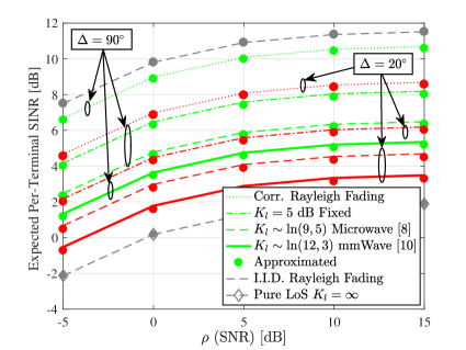
Figure 1: Expected per-terminal SNR vs. $\rho$ (SNR) with $M=32,L=3$ and $\Delta=20^{\circ}$ and $90^{\circ}$.

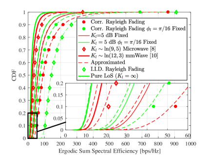
Figure 2: Ergodic sum spectral efficiency CDF with $M=256,L=32$ at $\rho=10$ dB and $\Delta=20^{\circ}$.

VI Conclusion

We have presented a general, yet insightful approximation to the expected per-terminal SINR and ergodic sum spectral efficiency of an uplink MU-MIMO system. With a ULA and MRC at the BS, the approximation is robust to equal and unequal correlation matrices, unequal levels of LoS, unequal link gains, unequal operating SNRs and system dimensions. With both microwave and mmWave parameters, our results show that unequal correlation matrices yield higher expected SINRs and ergodic sum spectral efficiency in comparison to equal correlation. Moreover, increasing the LoS component of the channel reduces the expected SINR and ergodic sum spectral efficiency due to the loss of spatial diversity.

Appendix A Proof of Lemma 1

We begin by recognizing that $\delta_{l}=\mathbb{E}\left[||\bm{g}_{l}||^{4}\right]=\mathbb{E}[\left(||\bm{g}_{l}||^{2}\right)^{2}]$. Substituting the definition of $\bm{g}_{l}$ and denoting $\bm{v}_{l}=\gamma_{l}\bm{R}_{l}^{\frac{1}{2}}\tilde{\bm{h}}_{l}$ and $\bm{q}_{l}=\eta_{l}\bar{\bm{h}}_{l}$ allows us to state

$$\delta_{l}=\mathbb{E}\left[\left(||\bm{g}_{l}||^{2}\right)^{2}\right]=\mathbb{E}\left[\left(\bm{v}_{l}^{\textrm{H}}\bm{v}_{l}+\bm{v}_{l}^{\textrm{H}}\bm{q}_{l}+\bm{q}_{l}^{\textrm{H}}\bm{v}_{l}+\bm{q}_{l}^{\textrm{H}}\bm{q}_{l}\right)^{2}\right].\vspace{-3pt}$$ (15)

Expanding (15) allows us to write

$$\delta_{l} =\hskip 1.0pt\mathbb{E}\left[\left(\bm{v}_{l}^{\textrm{H}}\bm{v}_{l}\right)^{2}+2\left(\bm{v}_{l}^{\textrm{H}}\bm{v}_{l}\right)\left(\bm{q}_{l}^{\textrm{H}}\bm{q}_{l}\right)+\left(\bm{v}_{l}^{\textrm{H}}\bm{q}_{l}\bm{q}_{l}^{\textrm{H}}\bm{v}_{l}\right)\right.$$

$$\left.+\left(\bm{q}_{l}^{\textrm{H}}\bm{v}_{l}\bm{v}_{l}^{\textrm{H}}\bm{q}_{l}\right)+\left(\bm{q}_{l}^{\textrm{H}}\bm{q}_{l}\right)^{2}\right].$$ (16)

Performing the expectations over $\bm{v}_{l}$ in the last four terms of (16) and simplifying yields

$$\delta_{l} =\mathbb{E}\left[\left(\bm{v}_{l}^{\textrm{H}}\bm{v}_{l}\right)^{2}\right]+2M\left(\eta_{l}\right)^{2}\left(\bm{q}_{l}^{\textrm{H}}\bm{q}_{l}\right)$$

$$+2\left(\eta_{l}\right)^{2}\bm{q}_{l}^{\textrm{H}}\bm{R}_{l}\bm{q}_{l}+\left(\bm{q}_{l}^{\textrm{H}}\bm{q}_{l}\right)^{2}.$$ (17)

After noting that $\mathbb{E}\big{[}\big{(}\bm{v}_{l}^{\textrm{H}}\bm{v}_{l}\big{)}^{2}\big{]}=\mathbb{E}\left[\bm{v}_{l}^{\textrm{H}}\bm{v}_{l}\bm{v}_{l}^{\textrm{H}}\bm{v}_{l}\right]$, substituting the definition of $\bm{v}_{l}$ and extracting the relevant constants yields $\mathbb{E}\big{[}\big{(}\bm{v}_{l}^{\textrm{H}}\bm{v}_{l}\big{)}^{2}\big{]}=\big{(}\eta_{l}\big{)}^{4}\mathbb{E}\big{[}\big{(}\tilde{\bm{h}}_{l}^{\textrm{H}}\bm{R}_{l}\tilde{\bm{h}}_{l}\big{)}^{2}\big{]}$, where $\bm{R}_{l}=\bm{\Phi\Lambda\Phi}^{\textrm{H}}$ via an eigenvalue decomposition. Hence,

$$\mathbb{E}\left[\left(\bm{v}_{l}^{\textrm{H}}\bm{v}_{l}\right)^{2}\right]=\left(\eta_{l}\right)^{4}\mathbb{E}\left[\hskip 2.0pt\left(\sum\nolimits_{i=1}^{M}\left[\bm{\Lambda}\right]_{i,i}\left|\left(\tilde{\bm{h}}_{l}\right)_{i}\right|^{2}\right)^{2}\right].\vspace{-10pt}$$ (18)

Performing the expectation with respect to $\tilde{\bm{h}}_{l}$ and simplifying yields $\mathbb{E}[(\bm{v}_{l}^{\textrm{H}}\bm{v}_{l})^{2}]=(\eta_{l})^{4}\{(\textrm{tr}\left[\bm{R}_{l}])^{2}+\textrm{tr}\left[\bm{R}_{l}^{2}\right]\right\}$. As $\textrm{tr}\left[\bm{R}_{l}\right]=M$, $\mathbb{E}[(\bm{v}_{l}^{\textrm{H}}\bm{v}_{l})^{2}]=\left(\eta_{l}\right)^{4}\{M^{2}+\textrm{tr}[(\bm{R}_{l})^{2}]\}$. Substituting the right-hand side along with the definition of $\bm{q}_{l}$ into (17), recognizing $\bar{\bm{h}}_{l}^{\textrm{H}}\bar{\bm{h}}_{l}=M$ and simplifying yields Lemma 1.

Appendix B Proof of Lemma 2

Applying the definition of $\bm{g}_{l}$ and $\bm{g}_{k}$ into $\varphi_{l,k}=\mathbb{E}\left[|\bm{g}_{l}^{\textrm{H}}\bm{g}_{k}|^{2}\right]$ and denoting $\bm{v}_{l}=\eta_{l}\bm{R}_{l}^{\frac{1}{2}}\tilde{\bm{h}}_{l}$ and $\bm{q}_{l}=\gamma_{l}\bar{\bm{h}}_{l}$ yields $\varphi_{l,k}=\mathbb{E}\left[\hskip 1.0pt\left|\hskip 1.0pt\left(\bm{v}_{l}^{\textrm{H}}+\bm{q}_{l}^{\textrm{H}}\right)\left(\bm{v}_{k}+\bar{\bm{h}}_{k}\right)\right|^{2}\right]$. Expanding and simplifying further gives

$$\varphi_{l,k} =\hskip 2.0pt\mathbb{E}\left[\bm{v}_{l}^{\textrm{H}}\bm{v}_{k}\bm{v}_{k}^{\textrm{H}}\bm{v}_{l}\right]+\mathbb{E}\left[\bm{v}_{l}^{\textrm{H}}\bm{q}_{k}\bm{q}_{k}^{\textrm{H}}\bm{v}_{l}\right]$$

$$+\mathbb{E}\left[\bm{q}_{l}^{\textrm{H}}\bm{v}_{k}\bm{v}_{k}^{\textrm{H}}\bm{q}_{l}\right]+\mathbb{E}\left[\bm{q}_{l}^{\textrm{H}}\bm{q}_{k}\bm{q}_{k}^{\textrm{H}}\bm{q}_{l}\right].$$ (19)

Recognizing that $\mathbb{E}\left[\bm{v}_{l}\bm{v}_{l}^{\textrm{H}}\right]=\mathbb{E}\left[\eta_{l}\bm{R}_{l}^{\frac{1}{2}}\tilde{\bm{h}}_{l}\eta_{l}\tilde{\bm{h}}_{l}^{\textrm{H}}\bm{R}_{l}^{\frac{1}{2}}\right]=\left(\eta_{l}\right)^{2}\bm{R}_{l}$, substituting back the definitions of $\bm{v}_{l}$, $\bm{v}_{k}$, $\bm{q}_{l}$ and $\bm{q}_{k}$ in (19) and extracting the relevant constants yields

$$\varphi_{l,k} \hskip 2.0pt=\left(\eta_{l}\right)^{2}\left(\eta_{k}\right)^{2}\textrm{tr}\left[\bm{R}_{k}\bm{R}_{l}\right]$$

$$+\left(\eta_{l}\right)^{2}\left(\gamma_{k}\right)^{2}\mathbb{E}\left[\textrm{tr}\left[\bm{R}_{l}^{\frac{1}{2}}\bar{\bm{h}}_{k}\bar{\bm{h}}_{k}^{\textrm{H}}\bm{R}_{l}^{\frac{1}{2}}\tilde{\bm{h}}_{l}\tilde{\bm{h}}_{l}^{\textrm{H}}\right]\right]$$

$$+\left(\gamma_{l}\right)^{2}\left(\eta_{k}\right)^{2}\mathbb{E}\left[\textrm{tr}\left[\tilde{\bm{h}}_{k}\tilde{\bm{h}}_{k}^{\textrm{H}}\bm{R}_{k}^{\frac{1}{2}}\bar{\bm{h}}_{l}\bar{\bm{h}}_{l}^{\textrm{H}}\bm{R}_{k}^{\frac{1}{2}}\right]\right]$$

$$+\left(\gamma_{l}\right)^{2}\left(\gamma_{k}\right)^{2}|\bar{\bm{h}}_{l}^{\textrm{H}}\bar{\bm{h}}_{k}|^{2}.\vspace{-5pt}$$ (20)

Taking the trace and simplifying yields (6).

References

• [1] F. Rusek, D. Persson, B. Lau, E. G. Larsson, T. L. Marzetta, O. Edfors, and F. Tufvesson, “Scaling up MIMO: Opportunities and challenges with very large arrays," IEEE Signal Process. Mag., vol. 30, no. 1, pp. 40-60, Nov. 2013.
• [2] J. Hoydis, S. ten Brink, and M. Debbah “Massive MIMO in the UL/DL of cellular networks: How many antennas do we need?," IEEE J. Sel. Areas Commun., vol. 31, no. 2, pp. 160-171, Feb. 2013.
• [3] J. Zhang, L. Dai, M. Matthaiou, C. Masouros, and S. Jin, “On the spectral efficiency of space-constrained massive MIMO with linear receivers," in Proc. IEEE ICC, May 2016, pp. 1-6.
• [4] J. Nam, G. Caire, and J. Ha, “On the role of transmit correlation diversity in multiuser MIMO systems," IEEE Trans. Inf. Theory, vol. 63, no. 1, pp. 336-354, Jan. 2017.
• [5] H. Tataria, P. J. Smith, L. J. Greenstein, and P. A. Dmochowski, “Zero-forcing precoding performance in multiuser MIMO systems with heterogeneous Ricean fading," IEEE Wireless Commun. Lett., vol. 6, no. 1, pp. 74-77, Feb. 2017.
• [6] Q. Zhang, S. Jin, K-K. Wong, H. Zhu, and M. Matthaiou, “Power scaling of uplink massive MIMO systems with arbitrary-rank channel means," IEEE J. Sel. Topics Signal Process., vol. 8, no. 5, pp. 966-981, Nov. 2014.
• [7] H. Falconet and L. Sanguinetti, A. Kammoun, and M. Debbah, “Asymptotic analysis of downlink MISO systems over Rician fading channels," in Proc. IEEE ICASSP, Mar. 2016, pp. 3926-3930.
• [8] 3GPP TR 36.873 v12.0.0, Study on 3D channel models for LTE, 3GPP, Jun. 2015.
• [9] M. R. Akdeniz, Y. Liu, M. K. Samimi, S. Sun, S. Rangan, T. S. Rappaport, and E. Erkip, “Millimeter wave channel modeling and cellular capacity evaluation," IEEE J. Sel. Areas Commun., vol. 32, no. 6, pp. 1164-1179, Jun. 2014.
• [10] T. Thomas, H. C. Nguyen, G. R. MacCartney, and T. S. Rappaport, “3D mmWave channel model proposal," in Proc. IEEE VTC-Fall, Sep. 2014, pp. 1-6.
• [11] Z. Jiang, A. F. Molisch, G. Caire, and Z. Niu, “Achievable rates of FDD massive MIMO systems with spatial channel correlation," IEEE Trans. Wireless Commun., vol. 14, no. 5, pp. 2862-2882, May 2015.