Nonparametric weighted stochastic block models

Abstract

We present a Bayesian formulation of weighted stochastic block models that can be used to infer the large-scale modular structure of weighted networks, including their hierarchical organization. Our method is nonparametric, and thus does not require the prior knowledge of the number of groups or other dimensions of the model, which are instead inferred from data. We give a comprehensive treatment of different kinds of edge weights (i.e. continuous or discrete, signed or unsigned, bounded or unbounded), as well as arbitrary weight transformations, and describe an unsupervised model selection approach to choose the best network description. We illustrate the application of our method to a variety of empirical weighted networks, such as global migrations, voting patterns in congress, and neural connections in the human brain.

I Introduction

Many network systems lack a natural low-dimensional embedding from which we can readily extract their most prominent large-scale features. Instead, we have to infer this information from data, typically by decomposing the observed network into modules Fortunato (2010). A principled approach to perform this task is to formulate generative models that allow this modular decomposition to be found via statistical inference Peixoto (2017a). The most fundamental model used for this purpose is the stochastic block model (SBM) Holland et al. (1983), which groups nodes according to their probabilities of connection to the rest of the network. However, a central limitation of most SBM implementations is that they are defined strictly for simple or multigraphs. This means that they do not incorporate extra information on the edges, which are typically present in a variety of systems, and are required for an accurate representation of their structure. For example, to the existence of a route between two airports is associated a distance, to the biomass flow between two species in a food web is associated a flow magnitude, etc. In this work, we develop variations of the SBM that allow for this type of information on the edges to be incorporated into the network model and guide the partition of the nodes into groups in a statistically meaningful way.

We follow the same basic idea put forth by Aicher et al. Aicher et al. (2015), who adapted the SBM to weighted networks by including edge values as additional covariates. However, our approach diverges from Ref. Aicher et al. (2015) in key aspects. First, here we develop a nonparametric Bayesian approach, based on exact integrated likelihoods, that is capable of inferring the dimension of the model — e.g. the number of groups — from the data itself, without requiring it to be known a priori. This is achieved by departing from the canonical exponential family of distributions, and using instead microcanonical formulations that are easier to compute exactly and approach the canonical distributions asymptotically. Second, our approach also infers the hierarchical modular structure of the network, extending the nested SBM of Refs. Peixoto (2014a, 2017b) to the weighted case. The hierarchical nature of the model is implemented via structured Bayesian priors that have been shown to significantly decrease the tendency of the nonparametric approach to underfit Peixoto (2013) and are capable of uncovering small but statistically significant modules in large networks Peixoto (2014a, 2017b). And third, our approach is efficient, making use of MCMC sampling that requires only $O(E)$ operations per sweep, where $E$ is the number of edges in the network, independently of the number of groups.

This paper is organized as follows. In Sec. II we present our general approach, and in Sec. III we illustrate its use in a variety of empirical weighted network datasets. In Sec. IV we elaborate on the diverse models for edge weights based on basic properties (such as whether they are discrete or continuous, signed or unsigned, bounded or unbounded), show how these models can be extended via weight transformations, and how different models can be chosen via Bayesian model selection. We finalize in Sec. V with a discussion.

II Weighted SBMs via edge covariates

We consider generative models for networks that, in addition to the adjacency matrix $\bm{A}=\{A_{ij}\}$, also possess real or discrete edge covariates $\bm{x}=\{\bm{x}_{ij}\}$ on the edges. Without loss of generality, here we assume that the networks are multigraphs, i.e. $A_{ij}\in\mathbb{N}_{0}$, such that $\bm{x}_{ij}$ is a vector containing one weight for each parallel edge between nodes $i$ and $j$, and no weights if $A_{ij}=0$. Furthermore, we assume that the edge existence is decoupled from its weight, i.e. the non-existence of an edge is different from an edge with zero weight (the special case where the zeros of the adjacency matrix are considered values of the edge covariates can be recovered by using a complete graph in place of $\bm{A}$, and adapting $\bm{x}$ accordingly). As done in Ref. Aicher et al. (2015), we follow the underlying assumption of the SBM that the nodes are divided into $B$ groups, with $b_{i}\in\{1,\dots,B\}$ specifying the group membership of node $i$, and where in addition to the edge placement, the edge weights are sampled only according to the group memberships of their endpoints. Concretely, this means they are both sampled from parametric distributions that are conditioned only on the group memberships of the nodes i.e.

$$P(\bm{A},\bm{x}|\bm{\theta},\bm{\gamma},\bm{b})=P(\bm{x}|\bm{A},\bm{\gamma},\bm{b})P(\bm{A}|\bm{\theta},\bm{b})$$ (1)

with the covariates being sampled only on existing edges,

$$P(\bm{x}|\bm{A},\bm{\gamma},\bm{b}) =\prod_{r\leq s}P(\bm{x}_{rs}|\bm{\gamma}_{rs})$$ (2)

with $\bm{x}_{rs}=\{\bm{x}_{ij}|A_{ij}>0\land(b_{i},b_{j})=(r,s)\}$ being the covariates between groups $r$ and $s$, and where $\bm{\gamma}_{rs}$ is a set of parameters that govern the sampling of the weights between groups $r$ and $s$. The placement of the edges is done independently of the weights by choosing any SBM flavor with parameters $\bm{\theta}$; For example, with the degree-corrected SBM Karrer and Newman (2011) we would have

$$P(\bm{A}|\bm{\theta}=\{\bm{\lambda},\bm{\kappa}\},\bm{b})=\prod_{i<j}\frac{\mathrm{e}^{-\lambda_{b_{i},bj}\kappa_{i}\kappa_{j}}(\lambda_{b_{i},bj}\kappa_{i}\kappa_{j})^{A_{ij}}}{A_{ij}!},$$ (3)

where $\lambda_{rs}$ controls the number of edges that are placed between groups, and $\kappa_{i}$ the expected degree of node $i$.

Given the generative model above, we could proceeded by estimating the parameters $\bm{\theta}$ and $\bm{\gamma}$ via maximum likelihood. However, doing so would be subject to overfitting, as the likelihood would increase monotonically with the complexity of the model. Instead, here we are interested in solving a more general and arguably more well-posed problem, namely to obtain the Bayesian posterior probability of partitions, in a nonparametric manner, taking into account only the weighted network,

$$P(\bm{b}|\bm{A},\bm{x})=\frac{P(\bm{A},\bm{x}|\bm{b})P(\bm{b})}{P(\bm{A},\bm{x})},$$ (4)

where the numerator contains the marginal likelihood integrated over the model parameters

$$P(\bm{A},\bm{x}|\bm{b}) =\int P(\bm{A},\bm{x}|\bm{\theta},\bm{\gamma},\bm{b})P(\bm{\theta})P(\bm{\gamma})\,\mathrm{d}\bm{\theta}\mathrm{d}\bm{\gamma}$$

$$=P(\bm{A}|\bm{b})P(\bm{x}|\bm{A},\bm{b}),$$ (5)

and where

$$P(\bm{A}|\bm{b})=\int P(\bm{A}|\bm{\theta},\bm{b})P(\bm{\theta})\,\mathrm{d}\bm{\theta}$$ (6)

is the marginal likelihood of the unweighted network integrated over the relevant parameters. Integrated marginal likelihoods of this kind were considered in numerous works for several unweighted model variants Guimerà and Sales-Pardo (2009); Yan et al. (2010); Peixoto (2013, 2014a); Côme and Latouche (2015); Newman and Reinert (2016); Peixoto (2017b). In this work, our approach is fully independent of any particular choice made for this part of the model. However, in our experiments we will use the nested microcanonical degree-corrected SBM described in Ref. Peixoto (2014a, 2017b), due to its efficient and multi-scale nature, as well as a much reduced tendency to underfit when used with large networks. Furthermore, its hierarchical nature will allow us to describe summaries of the network — taking into accounts its edge covariates — at multiple scales, providing a bird’s-eye view of large datasets. We use this model without sacrificing generality, since the usual non-hierarchical SBM amounts exactly to using the nested version with just one hierarchical level.

The crucial part in Eq. 5 that completes our nonparametric approach is the marginal likelihood of the edge weights, which is integrated over the weight parameters $\bm{\gamma}$ according to their prior distribution $P(\bm{\gamma}_{rs})$, which is the same for every pair of groups $r$ and $s$,

$$P(\bm{x}|\bm{A},\bm{b}) =\int P(\bm{x}|\bm{A},\bm{\gamma},\bm{b})P(\bm{\gamma})\,\mathrm{d}\bm{\gamma}$$

$$=\prod_{r\leq s}\int P(\bm{x}_{rs}|\bm{\gamma}_{rs})P(\bm{\gamma}_{rs})\,\mathrm{d}\bm{\gamma}_{rs}.$$ (7)

The form of the prior distribution $P(\bm{\gamma})$ is usually conditioned on hyperparameters $\bm{\eta}$, which represent our a priori assumptions about the data. In order for our inference approach to retain its nonparametric character, we need these hyperparameters to take a single global value, i.e. $P(\bm{\gamma}_{rs})=P(\bm{\gamma}_{rs}|\bm{\eta})$ for all groups $r$ and $s$. Alternatively, we may treat $\bm{\eta}$ as latent variables, and sample them from their own distribution, $P(\bm{\eta})$, thereby reducing the sensitivity to our a priori assumptions. This idea fits well with the nested version of the SBM we will be using Peixoto (2014a, 2017b), which, as part of its prior probabilities, considers the groups themselves as nodes of a smaller multigraph that is also generated by the SBM, with its nodes put in their own groups, forming an even smaller multigraph, and so on recursively, following a nested hierarchy $\{\bm{b}^{l}\}=\{\{b_{r}^{(l)}\}_{l}\}$, so that $b_{r}^{(l)}\in\{1,\dots,B_{l}\}$ is the group membership of group/node $r$ at the hierarchy level $l\in\{1,\dots,L\}$, with the boundary condition that the number of groups at the topmost level $l=L$ is $B_{L}=1$ (see Fig. 1 in Ref. Peixoto (2014a) for an illustration of the generative process). Therefore, the adjacency of the multigraph at level $l$ is

$$m_{rs}^{l}=\sum_{tu}\frac{m_{tu}^{l-1}\delta_{b^{(l)}_{t},r}\delta_{b^{(l)}_{u},s}}{\delta_{rs}+1},$$ (8)

where we assume $m_{ij}^{0}=A_{ij}$. Following the same logic, we may consider the parameters $\bm{\gamma}$ as edge covariates in the multigraph of groups, which themselves are generated by another model in a level above, and so on. We may thus let $\bm{\gamma}^{1}\equiv\bm{\gamma}$ and $\bm{\gamma}^{2}\equiv\bm{\eta}$ be the first two levels of a hierarchical model, given recursively by

$$P(\bm{\gamma}^{l}|\bm{A},\bm{b}^{l+1},\bm{\gamma}^{l+1})=\prod_{t\leq u}P(\bm{\gamma}_{tu}^{l}|\bm{A},\bm{b}^{l+1},\bm{\gamma}^{l+1}_{b_{t}^{(l+1)},b_{u}^{(l+1)}}),$$ (9)

where $\bm{\gamma}_{tu}^{l+1}=\{\bm{\gamma}_{rs}^{l}|m_{rs}^{l}>0\land(b_{r}^{(l+1)},b_{s}^{(l+1)})=(t,u)\}$ are the hyperparameters between groups $(t,u)$ at level $l+1$, with $m_{rs}^{l}$ given by Eq. 8. The final model is then obtained by integrating over the entire hierarchy,

$$P(\bm{x}|\bm{A},\{\bm{b}^{l}\})=\\ \int P(\bm{x}|\bm{A},\bm{\gamma}^{1},\bm{b}^{1})\prod_{l=1}^{L}P(\bm{\gamma}^{l}|\bm{A},\bm{\gamma}^{l+1},\bm{b}^{l+1})\;\mathrm{d}\bm{\gamma}^{l},$$ (10)

assuming the boundary condition $\bm{\gamma}^{L+1}=\{\hat{\bm{\gamma}}\}$, such that $\hat{\bm{\gamma}}$ is a single set of hyperparameters that are left out of the integration at the topmost level, reflecting only global aspects of the covariates, without a significant effect on the model structure and dimension. Instead of defining a unique model, we will consider a variety of elementary choices for $P(\bm{x}|\bm{\gamma})$ and $P(\bm{\gamma})$ that reflect the precise nature of the covariates (e.g. continuous or discrete, signed or unsigned, bounded or unbounded), and for which Eq. 10 can be computed exactly. In particular, we will make use of microcanonical formulations of the weight distributions that permit the straightforward computation of the integrals, without sacrificing descriptive power. We leave the derivations of the likelihood expressions for Sec. IV, and we proceed with a general outline, and an analysis of this approach for empirical networks.

When using the nested model, we have a posterior distribution over hierarchical partitions,

$$P(\{\bm{b}^{l}\}|\bm{A},\bm{x})=\frac{P(\bm{A},\bm{x}|\{\bm{b}^{l}\})P(\{\bm{b}^{l}\})}{P(\bm{A},\bm{x})},$$ (11)

which can be marginalized, if we so desire, to obtain only the partition at the bottom level $\bm{b}\equiv\bm{b}^{1}$,

$$P(\bm{b}|\bm{A},\bm{x})=\sum_{\{\bm{b}^{l}|\,l>1\}}P(\{\bm{b}^{l}\}|\bm{A},\bm{x}).$$ (12)

However, most typically we will want to obtain the entire hierarchical partition, as it is useful for a multilevel description of the data. Since the posterior in Eq. 11 involves a prior probability of the partition $P(\{\bm{b}^{l}\})$ (described in detail in Ref. Peixoto (2017b)), and is integrated over all remaining model parameters, it possesses an inherent regularization property, where overly complicated models are penalized with a lower posterior probability Jaynes (2003). This means that, differently from maximum likelihood approaches, we can infer properties related to the size of the model, such as the number of groups $B$ and hierarchy depth $L$, without danger of overfitting. Furthermore, as we detail further in Sec. IV.7, the posterior distribution gives us a principled means of model selection according to statistical significance, which allows us to choose the most appropriate weight model.

Given a choice for the parametric model for weights, we compute Eq. 10, which allows us to determine the posterior distribution of the partitions in Eq. 11 up to the normalizing constant $P(\bm{A},\bm{x})$ in the denominator, which is generally intractable. But since we cannot sample from the posterior distribution directly even if we could somehow compute this constant, we must resort to MCMC importance sampling methods, for which this normalizing constant is luckily not needed. Since the values that need to be inferred are only the hierarchical labels $\{\bm{b}^{l}\}$, we can use the exact same algorithm developed for the unweighted case in Refs. Peixoto (2014b, 2017b), which we summarize here. This is generally implemented by making move proposals $\{\bm{b}^{l}\}\to\{\bm{b}^{l}\}^{\prime}$ with probability $P(\{\bm{b}^{l}\}^{\prime}|\{\bm{b}^{l}\})$, and rejecting the proposal with probability $1-a$, where $a$ is the Metropolis-Hastings Metropolis et al. (1953); Hastings (1970) criterion

$$a =\operatorname{min}\left(1,\frac{P(\{\bm{b}^{l}\}^{\prime}|\bm{A},\bm{x})}{P(\{\bm{b}^{l}\}|\bm{A},\bm{x})}\frac{P(\{\bm{b}^{l}\}|\{\bm{b}^{l}\}^{\prime})}{P(\{\bm{b}^{l}\}^{\prime}|\{\bm{b}^{l}\})}\right).$$ (13)

Since the ratio in Eq. 13 does not depend on the normalization constant $P(\bm{A},\bm{x})$, the value of $a$ can be computed exactly, and — as long as the move proposals are ergodic — the algorithm above will eventually sample partitions from the desired posterior distribution asymptotically. We can also obtain the most likely hierarchical partition,

$$\{\bm{b}^{l}\}^{*}=\underset{\{\bm{b}^{l}\}}{\operatorname{argmax}}\,P(\{\bm{b}^{l}\}|\bm{A},\bm{x})$$ (14)

by replacing $P(\{\bm{b}^{l}\}|\bm{A},\bm{x})\to P(\{\bm{b}^{l}\}|\bm{A},\bm{x})^{\beta}$ in Eq. 13 and making $\beta\to\infty$ in slow increments. Therefore, we can both maximize and sample from the posterior distribution, using the same algorithm. In this work we use the same move proposals defined in Refs. Peixoto (2014b, 2017b) where we select the layer $l$ and a node $u$ in that layer, both randomly, and use the local information of the node’s neighbourhood combined with global information on that layer to propose a plausible move candidate for its group membership, $b^{l}_{u}\to r$, thereby improving equilibration speed (see Ref. Peixoto (2017b) for details). Additionally, in order to avoid getting trapped in metastable states, we employ the agglomerative initialization heuristic described in Ref. Peixoto (2014b) and extended to the nested model in Ref. Peixoto (2014a). The combination of these move proposals with the likelihood of the microcanonical SBM of Ref. Peixoto (2017b), as well as any of the weight likelihoods defined in Sec. IV, yields an algorithm where each MCMC sweep (i.e. for every node one move is attempted) is performed in time $O(E)$, independently of how many groups are occupied with nodes. For more details of the algorithm we defer to Refs. Peixoto (2014b, 2017b) and to the freely available C++ implementation in the graph-tool Python library Peixoto (2014c).

III Empirical networks

III.1 Migrations between countries

\begin{overpic}[width=195.12767pt]{best-fit-dataun-migration-2015-countries-net-weightedFalse.jpg}\put(0.0,0.0){(a)}\end{overpic}

\begin{overpic}[width=195.12767pt]{best-fit-dataun-migration-2015-countries-net-weightedTrue.jpg}\put(0.0,0.0){(b)}\end{overpic}

Figure 1: (a) Fit of the unweighted SBM for UN migration data, using the threshold approach described in the text. The edges are routed according the inferred hierarchy (shown in blue), using an edge-bundling algorithm by Holten Holten (2006), and the edge sources are marked with a green color. (b) Fit of the weighted SBM for the same data with the migrant stocks included, as shown by the edge colors and in the legend.

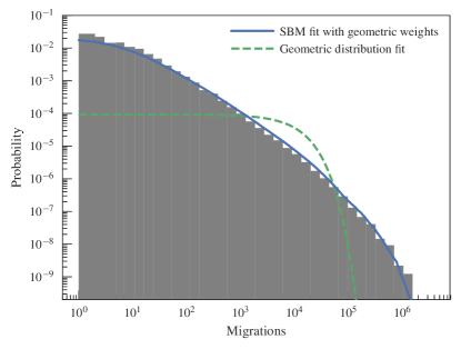
Figure 2: Overall distribution of the number of migrations for the UN data. The solid line shows the inferred distribution according to the weighted SBM using geometric distributions. The dashed line shows the best fit of a single geometric distribution.

\begin{overpic}[width=143.09538pt]{best-fit-datacamara-2009-weightedTrue-matrix.pdf}\put(0.0,0.0){(a)}\end{overpic}

\begin{overpic}[width=112.73882pt,trim=0.0pt -28.45274pt 0.0pt 0.0pt]{best-fit-datacamara-2009-weightedTrue-annotated.pdf}\put(0.0,0.0){(b)}\end{overpic}

\begin{overpic}[width=138.76157pt]{weight-dist-datacamara-2009.pdf}\put(0.0,0.0){(c)}\end{overpic}

Figure 3: (a) Fit of the weighted SBM for a matrix of vote correlations between deputies of the lower house of the Brazilian congress. The group boundaries are shown by horizontal and vertical lines. (b) Same as in (a) but using the layout of Fig. 1 that shows the entire hierarchical division. (c) Overall distribution of vote correlations. The solid line shows the inferred distribution according to the weighted SBM using transformed normal distributions. The dashed line shows the best fit using the same model, but on the shuffled data with the same empirical distribution.

We begin with an illustration of how incorporating edge weights with our method can have a significant effect on the analysis of network data. We use for this purpose a dataset of global migrations between $N=232$ countries, assembled in 2015 by the United Nations . This dataset can be represented as a directed network (see Appendix A), where for a pair of countries $(i,j)$ there is a net migrant stock $x_{ij}\in\mathbb{Z}$ which is defined as the number of migrants that moved from $i$ to $j$ minus the number that moved from $j$ to $i$. If we only had an unweighted SBM at our disposal, a common approach would be to threshold this data, yielding a directed edge $A_{ij}=1$ if $x_{ij}>0$ and $A_{ij}=0$ otherwise. As argued by Aicher et al Aicher et al. (2015), this type of data manipulation should be avoided whenever possible, since not only it destroys potentially valuable information, but also it is possible to construct examples where no single threshold can accurately reproduce the large-scale structure in the data. In this particular case, this approach actually does seem to yield usable information at first, as can be seen in Fig. 1a, which shows a fit of the unweighted SBM. We can see that the network division obtained in this manner essentially categorizes countries on whether they are net sources or targets of migration, as well as the typical regions people migrate to and from. However, a closer inspection reveals that it is not able to distinguish between countries like Costa Rica, South Africa and Finland (which end up clustered in the same group as Austria and Ireland), which not only are geographically far apart, but do have, in fact, very distinct migration volumes and patterns. Since migration volumes between countries can vary by several orders of magnitude (see Fig. 2), any analysis that ignores this aspect must be woefully incomplete. Indeed, if we include the values $x_{ij}$ of the migrant stock, in addition to the same adjacency matrix obtained with the threshold approach, and we use the weighted SBM defined previously, with geometric distributions for the weights as described in Sec IV.3, we obtain a much more detailed representation of the data, as shown in Fig. 1b. Not only we find a larger number of groups, but now countries like France, Canada and United Kingdom appear as members of very specific groups. The United States of America gets placed in its own group, due its unique volume and pattern of (mostly incoming) migrations. The remaining countries end up divided in geographically meaningful categories, with regions like South America, Middle East, Africa and Asia being easily recognizable. However, there are exceptions to this, where geographically separated countries get clustered together. Examples of this include Germany and India, as well as China and South Africa. These countries are either sources or targets of global migration which goes well beyond their immediate neighborhoods, and they possess similar overall patterns despite geographical distance (we emphasize that due to the degree-corrected nature of our model, countries with distinct migration balances can be put in the same category, if their group affinities are the same).

We can also assess the quality of the SBM in capturing the overall weight distribution, computed from the model as

$$P(x|\bm{A},\bm{x},\{\bm{b}^{l}\})=\frac{1}{E}\sum_{r\leq s}m_{rs}^{1}P(x|\bar{\bm{\gamma}}_{rs}^{1}),$$ (15)

with $E=\sum_{r\leq s}m_{rs}^{1}$ being the total number of edges, and $P(x|\bar{\bm{\gamma}}_{rs}^{1})$ is the marginal covariate distribution between groups $r$ and $s$, which in this case is given by Eq. 69. From Fig. 2, we see that the overall inferred distribution — which is a particular mixture of geometric distributions — is capable of providing a very good fit of the empirical data, despite the fact it is much broader than any single geometric distribution (a best fit of which is shown for reference).

III.2 Vote correlations in congress

We move now to another example where methods for unweighted graphs are ill suited. We consider the voting patterns of $N=475$ members of the lower house of the Brazilian congress during 2009 : Each deputy voted “yes” or “no” on proposed laws during the legislative year, and based on this, we computed the normalized correlation between the votes $x_{ij}\in[-1,1]$ of deputies $i$ and $j$. Note that in this case we have an adjacency matrix which is a complete graph, i.e. $A_{ij}=1$ for all $i,j$, and any pairs with zero correlation are considered particular values of the covariates.

This time we skip any attempt at thresholding the data, and we move directly to the analysis using the weighted SBM. For this, we use the version with normal distributions described in Sec. IV.2, adapted to bounded weights via the variable transformation $y_{ij}=2\operatorname{arctanh}(x_{ij})$ that maps the intervals $[-1,1]\to[-\infty,\infty]$, as described in Sec. IV.6. As shown in Fig. 3a, the method uncovers many groups of deputies, which collectively can be divided into two overall groups at the highest hierarchical level. These two large groups are more correlated with their own members than with non-members. An inspection of the known party affiliations of the deputies reveals that these two overall groups correspond to the government and opposition, which tend to vote together either against or in favor of bills. If we again inspect the overall distribution of vote correlations, we see that the weighted SBM provides a very good fit, as seen in Fig. 3c. The model captures the bimodal nature of the vote correlations — with higher values corresponding to pairs of deputies belonging both to either the government or opposition, and lower values to pairs belonging to different factions. It should be emphasized that the quality of the fit is not merely an outcome of using a sufficiently large mixture of normal distributions, as we are not modelling the overall distribution directly. Instead, the distributions are tied to the division of the nodes into groups, and the quality of the overall fit shows that the distribution of weights is well correlated with this categorization. For comparison, we show in Fig. 3c the outcome of the same analysis where the exact same weights are used, but they are randomly shuffled across pairs of deputies, thereby destroying any group organization but preserving the overall weight distribution. In this case, the best SBM fit is composed of only one group, $B=1$, and the corresponding normal fit cannot capture the bimodal structure of the weights — although it is still present in the shuffled data, albeit in a manner which is completely uncorrelated with any partition of the deputies. Therefore a close match between the empirical weight distribution and the SBM fit like the one in Fig. 3c — as well as the one in Fig. 2 for the UN migration data — is a testament to the quality of the SBM ansatz in explaining the data, rather than of an arbitrary mix of elementary unimodal distributions.

\begin{overpic}[width=260.17464pt,trim=0.0pt -14.22636pt 0.0pt 0.0pt]{{best-fit-databudapest_connectome_3.0_238_0_mean-20p-weightedTrue-walt9}.png} \put(0.0,0.0){(a)} \put(40.0,98.0){Right hemisphere} \put(37.0,0.0){Left hemisphere} \end{overpic}

\begin{overpic}[width=138.76157pt]{{weight-dist-databudapest_connectome_3.0_238_0_mean-20p-walt9a}.pdf}\put(0.0,0.0){(b)}\end{overpic} \begin{overpic}[width=138.76157pt]{{weight-dist-databudapest_connectome_3.0_238_0_mean-20p-walt9b}.pdf}\put(0.0,0.0){(c)}\end{overpic}

Figure 4: (a) Inferred SBM for the human connectome, using electrical connectivity and fractional anisotropy as edge covariates. The text labels show the most frequent anatomical annotation inside each group at the lowest hierarchical level; (b) Empirical and fitted distribution of electrical connectivity of the edges; (c) Empirical and fitted distribution of fractional anisotropy of the edges.

\begin{overpic}[width=433.62pt]{{modularity-databudapest_connectome_3.0_238_0_mean-20p-weightedTrue-walt9}.pdf}\put(0.0,1.0){(a)}\end{overpic}

\begin{overpic}[width=433.62pt]{{modularity-dispersity-databudapest_connectome_3.0_238_0_mean-20p-weightedTrue-walt9}.pdf}\put(0.0,1.0){(b)}\end{overpic}

Figure 5: (a) Group assortativity $q_{r}$ (Eq. 19) for the lowest level of the hierarchy in Fig 4a, with groups labelled using the most frequent anatomical annotation. Blue circle (red square) markers correspond to the left (right) hemisphere. On the right axis is shown a histogram of the $q_{r}$ values, with a horizontal line marking the average $Q=\sum_{r}q_{r}/B\approx 0.13$. The inset shows the modularity value $Q_{l}$ as a function of the hierarchy level $l$. (b) Dispersion of $q_{r}$ values for groups that share the same anatomical annotation, as labelled in the x-axis.

III.3 The human brain

We now analyze empirical networks of interactions between parts of human the brain, using data from the Budapest Reference Connectome Szalkai et al. (2017) (which itself is based on primary data from the Human Connectome Project McNab et al. (2013)). This dataset corresponds to a consensus between 477 people, where an edge between two of $N=1,006$ pre-defined anatomical regions is considered to exist, i.e. $A_{ij}=1$, if neuronal fibers connecting these two regions have been detected in at least 20% of the individuals. In addition to this basic connectivity, we consider two edge covariates, averaged over individuals: The “electrical connectivity” $x_{ij}\in[0,\infty]$, defined as the number of recorded fibers divided by their length, and the fractional anisotropy Basser and Pierpaoli (1996), $y_{ij}\in[0,1]$, which is maximal if all fibers in the affected region go in the same direction in 3D space, or minimal if they all go in different directions. Indeed, we use this dataset as an opportunity to highlight that our method can also be used when there are multiple covariates available. This can be done in an intuitive manner by assuming that their generation is conditioned on the same network partition, but otherwise are independent, i.e.

$$P(\bm{x},\bm{y}|\bm{A},\{\bm{b}^{l}\})=P(\bm{x}|\bm{A},\{\bm{b}^{l}\})P(\bm{y}|\bm{A},\{\bm{b}^{l}\}).$$ (16)

We can then use the exact same algorithm to obtain the posterior $P(\{\bm{b}^{l}\}|\bm{A},\bm{x},\bm{y})$ by simply combining both terms for $\bm{x}$ and $\bm{y}$. This approach will use the information in both covariates simultaneously to inform the partition of the network. (This is easily extended for an arbitrary number of covariates, and hence yields a method that is also suitable for vector-valued covariates, which is supported in our reference implementation Peixoto (2014c).) In the following, we use normal models for the transformed covariates $\ln x_{ij}$ and $\operatorname{logit}(y_{ij})$.

When applied to the brain dataset, our method reveals the structure shown in Fig. 4a. It decomposes the network into left and right hemispheres at the topmost hierarchical level, and proceeds to subdivide it into smaller regions. The subdivisions in both hemispheres are similar but not quite identical, indicating imperfect bilateral symmetry. The divisions at the bottom level are well correlated with known anatomical divisions, as shown by the labels in Fig. 4a. Most often, our method finds subdivisions of anatomical regions — i.e. a single anatomical region is divided in one or more groups — which are then grouped together higher in the hierarchy. But we also find some regions that belong to the same anatomical group that end up classified in significantly different hierarchy branches, pointing to a further degree of heterogeneity inside anatomical regions. Since the various traditional approaches to determine such anatomical classification do not always take into account the local and global connectivity patterns (i.e. the actual connectome), our approach suggests an alternative or complementary method to perform such a task.

Like in the previous examples, the fit of the overall distributions of edge covariates provided by the SBM is reasonably convincing, as we see in Figs. 4b and c, indicating that these nontrivial distributions — which deviate significantly from the basic distributions used in the model — can be well explained by group-to-group mixtures.

III.3.1 Community structure?

The modular structure of the brain has been studied numerous times before, using a variety of methods (e.g. Meunier et al. (2010); Bassett et al. (2013); Betzel et al. (2013)). Most often, however, this is done by searching for assortative modules Newman (2003), i.e. groups of nodes more connected to themselves than with the rest of the network — a pattern commonly called community structure Girvan and Newman (2002); Fortunato (2010). In contrast, the approach developed here seeks to find groups of nodes that have similar probabilities of connection with the rest of the network (and to generate edge covariates), regardless if they form a community or not. Naturally, community structure is a special case of the general class of patterns that we consider, but our approach is capable of accommodating many others, such as core-peripheries and bipartiteness — in fact, any arbitrary kind of group affinities. This means that if the formation of assortative communities is the main driving mechanism responsible for the network structure, we should be able to detect it with our method, but otherwise it will prefer a non-assortative division. This makes it a more flexible and potentially more informative approach in comparison to typical community detection methods, which, by construction, will tend to omit non-assortative divisions, however important they may be, in favor of assortative ones. In the case of brain networks, very often the community detection approach used is the maximization of modularity Newman (2003), defined as

$$Q=\frac{1}{2E}\sum_{r}e_{rr}-\frac{e_{r}^{2}}{2E},$$ (17)

where $e_{rs}=m_{rs}(1+\delta_{rs})$ is the number of edges between groups $r$ and $s$ (or twice that if $r=s$), and $e_{r}=\sum_{s}e_{rs}$. As has been known for a long time Guimerà et al. (2004), and since then has become well understood Reichardt and Bornholdt (2006); Bagrow (2012); McDiarmid and Skerman (2013, 2016); Prokhorenkova et al. (2016), the direct maximization of $Q$ to detect communities will generically overfit, as it will misleadingly find many spurious communities and produce large $Q$ values for completely random networks, as well as arguably non-modular networks such as trees. Somewhat paradoxically, the same approach will also generically underfit, as it is incapable of detecting a number of communities larger than $\sqrt{2E}$ Fortunato and Barthélemy (2007), even if their presence is statistically significant. Because of these and other limitations, as well as its non-statistical nature, the unsupervised maximization of $Q$ to find communities is ill-advised in most contexts Fortunato and Hric (2016). In contrast, the approach presented here is free of both these problems: When applied to completely random networks, it will not uncover spurious groups not sufficiently backed by statistical evidence Peixoto (2013); and it is capable of detecting up to $\propto N/\log N$ groups Peixoto (2014a, 2017b), whenever they are present. Since we have principled guarantees that the modules uncovered with our method are statistically significant, we can then use the value of $Q$ to characterize the degree of assortativity of the modules found (rather than the quality of the partition). For the result shown in Fig. 4, we obtain $Q\approx 0.13$, which is typically considered a low value indicating weak community structure. We may understand this value in more detail by decomposing it as

$$Q=\frac{1}{B}\sum_{r}q_{r}$$ (18)

where

$$q_{r}=\frac{B}{2E}\left(e_{rr}-\frac{e_{r}^{2}}{2E}\right)$$ (19)

is the local assortativity of group $r$, with $q_{r}\in[-1,1]$. In Fig. 5a we show the values of $q_{r}$ for the modules inferred with our method, labelled according to most prominent anatomical classification. We see that while most values are positive, $q_{r}>0$, strictly indicating a degree of assortativity, they are distributed across a broad range — with regions like the Caudate nucleus (associated with motor functions) even showing dissortativity with $q_{r}<0$ — indicating that assortativity, although it is present, is not an overwhelmingly dominant descriptor of the large-scale structure (a similar point has been made recently Betzel et al. (2017) using the method of Ref. Aicher et al. (2015)). We note also that inferred groups that are associated with the same anatomical region sometimes possess very different assortativity, as shown in Fig. 5b. This gives us an insight as to why they were classified in different groups in the first place, and further corroborating the idea that specific anatomical regions have noticeable internal heterogeneity.

One might speculate that assortativity is just one of a diverse set of driving forces behind the network formation, and that inspecting a detailed model of the network might dilute its importance. Here we can can further exploit the multilevel nature of our inferred model to assess if assortativity becomes more relevant at higher levels of coarse-graining. We can do so by computing a different value $Q_{l}$ for each hierarchical level $l$, defined by replacing $m_{rs}\to m_{rs}^{l}$ in Eq. 17, where $m_{rs}^{l}$ is the number of edges between groups $r$ and $s$ at level $l$. As we can see in the inset of Fig. 5a, the values of $Q_{l}$ do significantly increase at higher levels, suggesting that assortativity might be an important mechanism for the most global structures of the network, but not as much for its sub-structures at a smaller scale.

IV Elementary models for edge weights

The central piece of the posterior distribution of hierarchical partitions of Eq. 11 is the joint marginal probability of the network adjacency and weights,

$$P(\bm{A},\bm{x}|\{\bm{b}^{l}\})=P(\bm{x}|\bm{A},\{\bm{b}^{l}\})P(\bm{A}|\{\bm{b}^{l}\}).$$ (20)

For the unweighted part, $P(\bm{A}|\{\bm{b}^{l}\})$, we use the family of unweighted nested SBMs developed in Ref. Peixoto (2014a, 2017b). The reader is referred to those references, as well as the more recent overview provided in Ref. Peixoto (2017a), for a detailed derivation of the unweighted marginal likelihood, which we omit here for conciseness. To complete the model, we need to determine the placement of edge weights given the adjacency matrix and the hierarchical partition, with probability $P(\bm{x}|\bm{A},\{\bm{b}^{l}\})$ given by Eq. 10, which depends on the nature of the edge covariates.

In this section we derive models for edge covariates based on basic properties, such as whether they are signed or unsigned, continuous or discrete, bounded or unbounded. In particular, we focus on formulations that allow the integrated marginal likelihood $P(\bm{x}|\bm{A},\{\bm{b}^{l}\})$ to be computed exactly. For some of the derivations, we will assume — for convenience of notation — that the graphs are simple, i.e. $A_{ij}\in\{0,1\}$. We do so without loss of generality, as the final expressions will also be valid for multigraphs. In all cases, we begin with the simpler case of only one hierarchical level, where $\{\bm{b}^{l}\}$ is replaced by a single node partition $\bm{b}$, and generalize thereafter.

IV.1 Continuous unsigned weights

If all we know about the edge weights is that they are continuous and positive, i.e. $x_{ij}>0$, a reasonable model is a maximum-entropy distribution with a fixed average, i.e. the exponential distribution

$$P(x|\lambda)=\lambda\mathrm{e}^{-\lambda x}.$$ (21)

Using this as the basis of our weighted SBM yields,

$$P(\bm{x}_{rs}|\bm{A},\bm{\lambda},\bm{b}) =\prod_{ij}P(x_{ij}|\lambda_{rs})^{\frac{A_{ij}\delta_{b_{i},r}\delta_{b_{i},s}}{1+\delta_{rs}}}$$ (22)

$$=\lambda_{rs}^{m_{rs}}\mathrm{e}^{-\lambda_{rs}\mu_{rs}},$$ (23)

with

$$\mu_{rs}=\sum_{ij}\frac{A_{ij}x_{ij}\delta_{b_{i},r}\delta_{b_{j},s}}{1+\delta_{rs}}$$ (24)

being the sum of the weights between groups $r$ and $s$. Before computing the integrated marginal likelihood of Eq. 7, we need to select a prior for $\bm{\lambda}$. A natural choice that makes the computation feasible is known as a conjugate prior, which in this case is the gamma distribution

$$P(\lambda|\alpha,\beta)=\frac{\beta^{\alpha}\lambda^{\alpha-1}}{\Gamma(\alpha)}\mathrm{e}^{-\lambda\beta},$$ (25)

where $\alpha$ and $\beta$ are hyperparameters controlling its shape. Using this prior, we can write the marginal likelihood for the network weights by integrating over all $\lambda_{rs}$, yielding

$$P(\bm{x}|\bm{A},\bm{b},\alpha,\beta)=\prod_{r\leq s}\frac{\Gamma(m_{rs}+\alpha)}{\Gamma(\alpha)}\frac{\beta^{\alpha}}{(\mu_{rs}+\beta)^{m_{rs}+\alpha}}.$$ (26)

Doing so, we have reduced the initially high number of parameters from $B(B+1)/2$ to only two, corresponding to the hyperparameters $\alpha$ and $\beta$. Being global parameters, independent of the internal dimension of the model, they can be chosen via maximum likelihood, without significant risk of overfitting,

$$\hat{\alpha},\hat{\beta}=\underset{\alpha,\beta}{\operatorname{argmax}}\;P(\bm{x}|\bm{A},\bm{b},\alpha,\beta),$$ (27)

which can be done efficiently with any standard optimization method. Alternatively, we may consider the choice $\alpha=1$, for which $P(\lambda|\alpha,\beta)$ becomes the maximum-entropy distribution with a fixed mean, and hence has the same shape as $P(x|\lambda)$. Even with this choice, however, is difficult to incorporate this prior in the nested SBM via Eq. 10, as the integration over the remaining hierarchical levels is cumbersome. Instead, we now describe a microcanonical formulation which generates covariates in an asymptotically identical manner, but permits the exact integration of Eq. 10.

IV.1.1 Microcanonical distribution

Instead of generating each covariate independently, we consider the uniform joint distribution of $N$ positive real values $\bm{x}=\{x_{1},\dots,x_{N}\}$ conditioned on their total sum $\mu=\sum_{i}x_{i}$,

$$P(\bm{x}|\mu)=\begin{cases}{\displaystyle\frac{(N-1)!}{\mu^{N-1}}}\delta(\mu-\sum_{i}x_{i})&\text{ if }\mu>0\\ \prod_{i}\delta(x_{i})&\text{ if }\mu=0,\end{cases}$$ (28)

where the normalization constant $(N-1)!/\mu^{N-1}$ above accounts for the volume of a scaled simplex of dimension $N-1$. Although the covariates are not generated independently in Eq. 28, the marginal distribution of the individual values $x_{i}$ can be obtained as

$$P(x_{i}|N,\mu) =\frac{P(\bm{x}|\mu)}{P(\bm{x}\setminus x_{i}|\mu-x_{i})},$$ (29)

$$=\frac{(N-1)(\mu-x_{i})^{N-2}}{\mu^{N-1}}\Theta(\mu-x_{i})$$ (30)

using Eq. 28 both in the numerator and denominator of Eq. 29, and $\Theta(x)$ is the Heaviside step function. Taking the limit $N\to\infty$ while keeping the mean $\bar{x}=\mu/N$ fixed, $P(x_{i}|N,\mu)$ becomes Eq. 21 with $\lambda=1/\bar{x}$ (see Fig. 6). Since in the limit of sufficient data both models become identical, the microcanonical model enables us to have an exact hierarchical SBM, as we will now show, without sacrificing descriptive power.

Incorporating the microcanonical model of Eq. 28 in the SBM amounts simply to

$$P(\bm{x}_{rs}|\bm{A},\bm{\lambda},\bm{b})=P(\bm{x}_{rs}|\mu_{rs}),\vspace{.5em}$$ (31)

where, as before, $\mu_{rs}$ is the sum of covariates between groups $r$ and $s$. To generate the parameters $\mu_{rs}$ — which are also non-negative real numbers — we can use the exact same distribution again at a higher hierarchical level, by treating them as edge covariates of the graph of groups, as described in Eq. 10. The microcanonical nature of this model makes the integration over all parameters $\{\bm{\mu}_{rs}^{l}\}$ trivial due to the hard constraints, i.e.

$$P(\bm{x}|\bm{A},\{\bm{b}^{l}\}) =\int P(\bm{x}|\bm{A},\bm{\mu}^{1},\bm{b}^{1})\prod_{l=1}^{L}\prod_{r\leq s}\left[P(\bm{\mu}^{l}_{rs}|\mu^{l+1}_{b_{r}^{(l+1)},b_{s}^{(l+1)}})\;\mathrm{d}\bm{\mu}^{l}_{rs}\right]^{1-\delta_{m_{rs}^{l},0}}$$ (32)

$$=\prod_{l=1}^{L}\prod_{r\leq s}\left[\frac{(m_{rs}^{l}-1)!}{(\bar{\mu}_{rs}^{l})^{m_{rs}^{l}-1}}\right]^{1-\delta_{\mu_{rs}^{l},0}},$$ (33)

where

$$\bar{\mu}_{rs}^{l}=\sum_{tu}\left(\frac{\bar{\mu}_{tu}^{l-1}\delta_{b_{t}^{l},r}\delta_{b_{u}^{l},s}}{1+\delta_{rs}}\right)^{1-\delta_{m_{tu}^{l},0}}$$ (34)

is the sum of covariates between groups $r$ and $s$ at level $l>1$, and with $\bar{\mu}_{rs}^{1}=\mu_{rs}$ given by Eq. 24 at the lowest level. Recall that the boundary condition used in Eq. 10 is that at the topmost level there is only one group, and hence $m_{rs}^{L}=E\delta_{r,1}\delta_{s,1}$ and $\bar{\mu}_{rs}^{L}=\hat{\mu}\delta_{r,1}\delta_{s,1}$, where $\hat{\mu}=\sum_{i<j}A_{ij}x_{ij}$ is the total sum of edge weights, and the sole remaining parameter of the model. The marginal likelihood of Eq. 33 is a simple term that can be computed easily by obtaining the covariate summaries at each level, and amounts to a straightforward modification of the algorithm of Ref. Peixoto (2017b) to obtain the posterior distribution of hierarchical partitions. In particular, this additional term does not affect its algorithm complexity, since changes in a lower hierarchical level that are compatible with the partition at higher level do not alter the likelihoods in the upper levels, as the covariate sums remain unchanged.

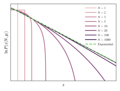
Figure 6: The marginal distribution of each individual covariate $x$ in the unsigned microcanonical model, given by Eq. 30, approaches asymptotically the exponential distribution as the number of values $N$ increases, and if the mean $\bar{x}=\mu/N$ is kept fixed.

IV.2 Continuous signed weights

For weights that can be either positive or negative, we require a maximum entropy distribution with fixed average and variance, which is the normal distribution

$$P(x|\bar{x},\sigma^{2})=\frac{1}{\sqrt{2\pi\sigma^{2}}}\mathrm{e}^{-\frac{(x-\bar{x})^{2}}{2\sigma^{2}}}.$$ (35)

Incorporating this in the SBM, we obtain

$$P(\bm{x}_{rs}|\bm{A},\bar{x}_{rs},\sigma^{2}_{rs}) =\prod_{ij}P(x_{ij}|\bar{x}_{rs},\sigma^{2}_{rs})^{\frac{A_{ij}\delta_{b_{i},r}\delta_{b_{i},s}}{1+\delta_{rs}}}$$ (36)

$$=\frac{\mathrm{e}^{-\frac{\nu_{rs}-2\mu_{rs}\bar{x}_{rs}+m_{rs}\bar{x}_{rs}^{2}}{2\sigma_{rs}^{2}}}}{(2\pi\sigma_{rs}^{2})^{m_{rs}/2}},$$ (37)

with

$$\nu_{rs}=\sum_{ij}\frac{A_{ij}x_{ij}^{2}\delta_{b_{i},r}\delta_{b_{j},s}}{1+\delta_{rs}}$$ (38)

being the sum of squares of covariates between groups $r$ and $s$. The conjugate prior for $\bar{x}$ and $\sigma^{2}$ is the normal-inverse-chi-squared distribution Box and Tiao (2011)

$$P(\bar{x},\sigma^{2}|\mu_{0},\kappa_{0},\nu_{0},\sigma^{2}_{0})=\mathcal{N}(\bar{x}|\mu_{0},\sigma^{2}/\kappa_{0})\chi^{-2}(\sigma^{2}|\nu_{0},\sigma^{2}_{0}),$$ (39)

where $\mathcal{N}(\bar{x}|a,b)$ is a normal distribution with mean $a$ and variance $b$, and the variance is sampled from an inverse-chi-squared distribution

$$\chi^{-2}(\sigma^{2}|\upsilon,\tau^{2})=\frac{(\tau^{2}\upsilon/2)^{\upsilon/2}}{\Gamma(\upsilon/2)}\leavevmode\nobreak\ \frac{\mathrm{e}^{\frac{-\upsilon\tau^{2}}{2\sigma^{2}}}}{\sigma^{2+\upsilon}}.$$ (40)

Using this prior, after the integration over $\bar{x}$ and $\sigma^{2}$, the marginal likelihood becomes

$$P(\bm{x}_{rs}|\bm{A},\mu_{0},\kappa_{0},\nu_{0},\sigma^{2}_{0})=\\ \frac{\Gamma(\nu_{rs}^{\prime}/2)}{\Gamma(\nu_{0}/2)}\sqrt{\frac{\kappa_{0}}{\kappa_{rs}}}\frac{(\nu_{0}\sigma^{2}_{0})^{\nu_{0}/2}}{(\nu_{rs}^{\prime}S_{rs})^{\nu_{rs}/2}}\frac{1}{\pi^{m_{rs}/2}},$$ (41)

with auxiliary quantities

$$\kappa_{rs} =\kappa_{0}+m_{rs},\quad\nu_{rs}^{\prime}=\nu_{0}+m_{rs},$$ (42)

$$z_{rs} =\nu_{rs}-\mu_{rs}^{2}/m_{rs},$$ (43)

$$S_{rs} =\frac{1}{\nu_{rs}^{\prime}}\left[\nu_{0}\sigma_{0}^{2}+z_{rs}+\frac{m_{rs}\kappa_{0}}{\kappa_{0}+m_{rs}}\left(\mu_{0}-\frac{\mu_{rs}}{m_{rs}}\right)^{2}\right].$$ (44)

This leaves us with four global parameters, $\mu_{0}$, $\kappa_{0}$, $\nu_{0}$ and $\sigma^{2}_{0}$, that we have to determine either with maximum likelihood, or maximum entropy arguments. However, like the unsigned case previously, the shape of the marginal likelihood leaves little chance of building a hierarchical model in closed form. Luckily, we can once more construct a microcanonical model that allows us do precisely that.

IV.2.1 Microcanonical distribution

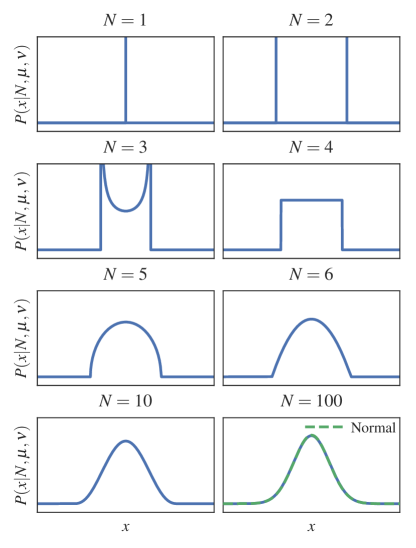
Figure 7: The marginal distribution of each individual covariate $x$ in the signed microcanonical model, given by Eq. 52, approaches asymptotically the normal distribution as the number of values $N$ increases, and if the mean $\bar{x}=\mu/N$ and variance $\sigma^{2}=\nu/N-\bar{x}^{2}$ are kept fixed.

The corresponding microcanonical maximum-entropy formulation for signed covariates is the uniform distribution of $N$ values $\bm{x}$ conditioned in the total sum $\mu$ and sum of squares $\nu$,

$$P(\bm{x}|\mu,\nu)=\frac{\delta(\mu-{\textstyle\sum_{i}x_{i}})\delta(\nu-{\textstyle\sum_{i}x_{i}^{2}})}{\Omega}.$$ (45)

The normalization constant is computed as

$$\Omega =\int\delta(\mu-{\textstyle\sum_{i}x_{i}})\delta(\nu-{\textstyle\sum_{i}x_{i}^{2}})\,\mathrm{d}\bm{x}$$ (46)

$$=\int_{H}\frac{\delta(\textstyle\nu-\sum_{i}x_{i}(\bm{y})^{2})}{\sqrt{N}}\,\mathrm{d}\bm{y}(\bm{x})$$ (47)

$$=\int_{S}\frac{\mathrm{d}\bm{\sigma}(\bm{x})}{2\sqrt{N\nu-\mu^{2}}}$$ (48)

$$=\frac{\pi^{(N-1)/2}\left(\nu-\mu^{2}/N\right)^{(N-3)/2}}{\Gamma(N/2-1/2)\sqrt{N}},$$ (49)

where $H$ in Eq. 47 is the hyperplane given by $\textstyle\sum_{i}x_{i}=\mu$, parametrized by $N-1$ coordinates $\bm{y}(\bm{x})$, and $S$ in Eq. 48 is the intersection of a $N$-sphere of radius $\sqrt{\nu}$ and the hyperplane $H$, which corresponds to the surface of a $(N-1)$-sphere of radius $\sqrt{\nu-\mu^{2}/N}$, with surface element $\mathrm{d}\bm{\sigma}(\bm{x})$, leading to Eq. 49. Therefore, we have for the complete microcanonical distribution

$$P(\bm{x}|\mu,\nu)=\\ \begin{cases}\displaystyle\frac{\displaystyle\Gamma(N/2-1/2)\sqrt{N}}{\displaystyle\pi^{(N-1)/2}(\nu-\mu^{2}/N)^{(N-3)/2}}\delta(\mu-{\textstyle\sum_{i}x_{i}})\delta(\nu-{\textstyle\sum_{i}x_{i}^{2}}),&\text{ if }\nu>\mu^{2}/N,\\ \prod_{i}\delta(\mu/N-x_{i}),&\text{ if }\nu=\mu^{2}/N.\end{cases}$$ (50)

The marginal distribution of the individual covariates $x_{i}$ can be obtained as

$$P(x_{i}|N,\mu,\nu) =\frac{P(\bm{x}|\mu,\nu)}{P(\bm{x}\setminus x_{i}|\mu-x_{i},\nu-x_{i}^{2})},$$ (51)

$$=\frac{\Gamma(N/2-1/2)}{\Gamma(N/2-1)}\sqrt{\frac{N}{\pi(N-1)}}\frac{[\nu-x_{i}^{2}-(\mu-x_{i})^{2}/(N-1)]^{N/2-2}}{(\nu-\mu^{2}/N)^{(N-3)/2}}\Theta(\mu-x_{i})\Theta(\nu-x_{i}^{2}),$$ (52)

using Eq. 50 both in the numerator and denominator of Eq. 51. Taking the limit $N\to\infty$ while keeping both the mean $\bar{x}=\mu/N$ and variance $\sigma^{2}=\nu/N-\bar{x}^{2}$ fixed, $P(x_{i}|N,\mu,\nu)$ becomes the normal distribution of Eq. 45 (see Fig. 7). Therefore, like with the unsigned case, the microcanonical model yields an easy-to-integrate model, without sacrificing descriptive power.

Incorporating the above distribution into the SBM yields

$$P(\bm{x}_{rs}|\bm{A},\bm{\mu},\bm{\nu},\bm{b})=P(\bm{x}_{rs}|\mu_{rs},\nu_{rs}),$$ (53)

where, as before, $\mu_{rs}$ is the sum of covariates between groups $r$ and $s$, and $\nu_{rs}$ is the sum of squares of the same covariates. To generate the parameters $\mu_{rs}$, we can use the exact same distribution again at a higher hierarchical level. The parameters $\nu_{rs}$, however, are strictly positive, and hence require a different model. Furthermore, $\mu_{rs}$ and $\nu_{rs}$ are not independent parameters, as they must satisfy the inequality $\nu_{rs}\geq\mu_{rs}^{2}/m_{rs}$. Therefore, we re-parametrize the model using the auxiliary quantity of Eq. 43

$$z_{rs}=\nu_{rs}-\mu_{rs}^{2}/m_{rs},$$ (54)

which is simply the scaled variance of the covariates, and thus is strictly non-negative and can be chosen independently from $\mu_{rs}$. We can then generate $z_{rs}$ from the unsigned microcanonical model of Eq. 28. Although we can easily write the final marginal likelihood of the model if we propagate the hyperpriors of $z_{rs}$ upwards in the hierarchy of the nested SBM, we would have the following problems: Not only this would increase the total number of edge covariates at the highest levels (and hence it is unclear a priori if it is the most parsimonious approach), since each signed parameter requires two hyperparameters, but also it leads to a model that is cumbersome computationally, as changes in a lower level would always propagate through the whole hierarchy. Instead, here we opt to propagate only $\mu_{rs}$ upwards in the hierarchy, whereas we generate all $z_{rs}$ from the same distribution at each level. More concretely, we write

$$P(\bm{x}|\bm{A},\{\bm{b}^{l}\}) =\int P(\bm{x}|\bm{A},\bm{\mu}^{1},\bm{z}^{1},\bm{b}^{1})P(\bm{\mu}_{z})\prod_{l=1}^{L}P(\bm{z}^{l}|\mu_{z}^{l})\prod_{r\leq s}\left[P(\bm{\mu}^{l}_{rs}|\mu^{l+1}_{b_{r}^{(l+1)},b_{s}^{(l+1)}},\bm{z}^{l+1}_{b_{r}^{(l+1)},b_{s}^{(l+1)}})\right]^{1-\delta_{m_{rs}^{l},0}}\;\mathrm{d}\bm{\mu}^{l}\mathrm{d}\bm{z}^{l}\mathrm{d}\mu_{z}^{l},$$ (55)

$$=\frac{(\bar{L}-1)!}{(\sum_{l=1}^{L}m_{z}^{l}\bar{\mu}_{z}^{l})^{\bar{L}-1}}\prod_{l=1}^{L}(m_{z}^{l})^{1-\delta_{m_{z}^{l},0}}\left[\frac{(m_{z}^{l}-1)!}{(\bar{\mu}_{z}^{l})^{m_{z}^{l}-1}}\right]^{1-\delta_{\bar{\mu}_{z}^{l},0}}\prod_{r\leq s}\left[\frac{\Gamma(m_{rs}^{l}/2-1/2)\sqrt{m_{rs}^{l}}}{\pi^{(m_{rs}^{l}-1)/2}(\bar{z}_{rs}^{l})^{(m_{rs}^{l}-3)/2}}\right]^{1-\delta_{\bar{z}_{rs}^{l},0}},$$ (56)

where $\bar{z}_{rs}^{l}=\bar{\nu}_{rs}^{l}-(\bar{\mu}_{rs}^{l})^{2}/m^{l}_{rs}$, with $\bar{\mu}_{rs}^{l}$ given by Eq. 34, and

$$\bar{\nu}_{rs}^{l}=\sum_{tu}\left[\frac{(\bar{\mu}_{tu}^{l-1})^{2}\delta_{b_{t}^{l},r}\delta_{b_{u}^{l},s}}{1+\delta_{rs}}\right]^{1-\delta_{m_{tu}^{l},0}},$$ (57)

corresponds to the scaled variance of the values of $\bar{\mu}_{rs}^{l-1}$ at a lower level (assuming the boundary conditions $\bar{\mu}_{rs}^{1}=\mu_{rs}$ and $\bar{\nu}_{rs}^{1}=\nu_{rs}$ given by Eqs. 24 and 38, respectively), and where

$$m_{z}^{l} =\sum_{r\leq s}H(m_{rs}^{l}-1),$$ (58)

$$\bar{\mu}_{z}^{l} =\sum_{r\leq s}\bar{z}_{rs}^{l}H(m_{rs}^{l}-1),$$ (59)

are the sum and scaled average $\bar{z}_{rs}^{l}$ of $m_{rs}^{l}>1$ entries at level $l$, with $H(x)=1$ if $x>0$, otherwise $H(x)=0$, and $P(\bm{z}^{l}|\mu_{z}^{l})$ is given by Eq. 28. The above means that when computing $P(\bm{z}^{l}|\mu_{z}^{l})$ we must only consider values of $z_{rs}^{l}$ for which $m_{rs}^{l}>1$. Otherwise, if $m_{rs}^{l}=1$, the corresponding parameter must always be $\nu_{rs}^{l}=(\mu_{rs}^{l})^{2}$, and hence $z_{rs}^{l}=0$, which does not need to be sampled from a prior. Finally, the values of $\bm{\mu}_{z}=\{\mu_{z}^{l}\}$ across all levels are also sampled from their own model as

$$P(\bm{\mu}_{z})=P(\{m_{z}^{l}\mu_{z}^{l}\}|{\textstyle\sum_{l=1}^{L}m_{z}^{l}\mu_{z}^{l}})\prod_{l=1}^{L}(m_{z}^{l})^{1-\delta_{m_{z}^{l},0}},$$ (60)

using again Eq. 28, and where the trailing product is a derivative term that accounts for the scaling of the variables in the argument of the first term, and with

$$\bar{L}=\sum_{l=1}^{L}H(m_{z}^{l})$$ (61)

being the number of levels with non-zero values of $m_{z}^{l}$. The boundary condition in Eqs. 10 and 55, i.e. that the last level of the hierarchy has only one group, means that the two remaining parameters are $\bar{\mu}_{rs}^{L}=\hat{\mu}\delta_{r,1}\delta_{s,1}$, where $\hat{\mu}=\sum_{i<j}A_{ij}x_{ij}$ is the total sum of edge weights, and $\hat{\mu}_{z}=\sum_{l}m_{z}^{l}\bar{\mu}_{z}^{l}$ which is the sum of scaled variances across the hierarchy levels.

Like with the unsigned model, Eq. 56 amounts to a straightforward modification of the algorithm of Ref. Peixoto (2017b), requiring only an additional book-keeping of the values of $z_{rs}^{l}$ for which $m_{rs}^{l}$ is larger than one, and their respective sums, which can be done without altering the overall algorithmic complexity. We remark also that, unlike maximum likelihood approaches applied directly to Eq. 45, the resulting marginal likelihood of the microcanonical model is well defined and yields non-degenerate results for any possible set of covariates, even those yielding zero variance or populations with single elements.

IV.3 Geometric discrete weights

For discrete non-negative weights, i.e. $x\in\mathbb{N}_{0}$, the maximum entropy distribution with a fixed average is the geometric distribution

$$P(x|p)=(1-p)^{x}p.$$ (62)

Using it for the SBM, we have

$$P(\bm{x}_{rs}|\bm{A},\bm{b},p_{rs})=(1-p_{rs})^{\mu_{rs}}p_{rs}^{m_{rs}}.$$ (63)

The conjugate prior for $p$ is the beta distribution

$$P(p|\alpha,\beta)=\frac{p^{\alpha-1}(1-p)^{\beta-1}}{B(\alpha,\beta)},$$ (64)

with $B(x,y)=\Gamma(x)\Gamma(y)/\Gamma(x+y)$, which yields the marginal distribution

$$P(\bm{x}_{rs}|\bm{A},\bm{b},\alpha,\beta)=\frac{B(m_{rs}+\alpha,\mu_{rs}+\beta)}{B(\alpha,\beta)}.$$ (65)

Unlike the continuous case, we can make a fully “uninformative” choice $\alpha=\beta=1$ that reflects our maximum ignorance about the parameter $p$, as in this case it is uniformly sampled in the interval $p\in[0,1]$. This yields simply

$$P(\bm{x}_{rs}|\bm{A},\bm{b})=\frac{m_{rs}!\,\mu_{rs}!}{(m_{rs}+\mu_{rs}+1)!}.$$ (66)

However, this kind of uninformative assumption rarely matches what we end up finding in the data, which tends to be significantly more structured. A more robust approach is to construct a hierarchical model, which can be more easily done with a microcanonical description.

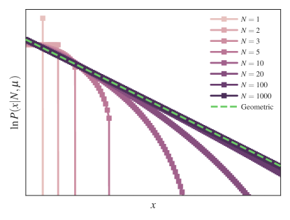
Figure 8: The marginal distribution of each individual covariate $x$ in the discrete microcanonical model, given by Eq. 69, approaches asymptotically the geometric distribution as the number of values $N$ increases, and the mean value $\mu/N$ is kept fixed.

IV.3.1 Microcanonical distribution

The microcanonical analogue of the geometric distribution is the uniform distribution of $N$ non-negative discrete real values $\bm{x}$ conditioned on their total sum $\mu$, given by

$$P(\bm{x}|\mu)=\left(\kern-3.00003pt\left(\genfrac{}{}{0.0pt}{}{N}{\mu}\right)\kern-3.00003pt\right)^{-1}\delta_{\mu,\sum_{i}x_{i}},$$ (67)

where $\left(\kern-3.00003pt\left(\genfrac{}{}{0.0pt}{}{N}{\mu}\right)\kern-3.00003pt\right)={N+\mu-1\choose\mu}$ counts the number of ways to distribute a total of $\mu$ values into $N$ distinguishable parts. The marginal distribution of the individual covariates $x_{i}$ can be obtained as

$$P(x_{i}|N,\mu) =\frac{P(\bm{x}|\mu)}{P(\bm{x}\setminus x_{i}|\mu-x_{i})},$$ (68)

$$=\frac{(N+\mu-x_{i}-1)!\mu!}{(N+\mu-1)!(\mu-x_{i})!}H(\mu-x_{i}).$$ (69)

Like with the continuous model, for sufficiently large $N$ and with the mean $\mu/N$ fixed, the marginal distribution of individual values $x_{i}$ will follow asymptotically a geometric distribution with $p=N/(\mu+N)$ (see Fig. 8).

Since the value of the parameter $\mu$ is also non-negative, we can sample it from the same distribution as a prior. Putting this in the SBM yields

$$P(\bm{x}|\bm{A},\bm{\mu}^{1},\bm{b}^{1})=\prod_{r\leq s}P(\bm{x}_{rs}^{1}|\mu_{rs}^{1})$$ (70)

and the final marginal distribution

$$P(\bm{x}|\bm{A},\{\bm{b}^{l}\})=\sum_{\{\mu^{l}_{rs}\}}P(\bm{x}|\bm{A},\bm{\mu}^{1},\bm{b}^{1})\prod_{l=1}^{L}\prod_{r\leq s}\left[P(\bm{\mu}^{l}_{rs}|\mu^{l+1}_{b_{r}^{(l+1)},b_{s}^{(l+1)}})\right]^{1-\delta_{m_{rs}^{l},0}}\\ =\prod_{l=1}^{L}\prod_{r\leq s}\left[\left(\kern-3.00003pt\left(\genfrac{}{}{0.0pt}{}{m_{rs}^{l}}{\bar{\mu}_{rs}^{l}}\right)\kern-3.00003pt\right)^{-1}\right]^{1-\delta_{\bar{\mu}_{rs}^{l},0}},$$ (71)

with $\bar{\mu}_{rs}^{l}$ given by Eq. 34. Like with the continuous models, the use of Eq. 71 requires only a simple modification of the algorithm of Ref. Peixoto (2017b), that does not alter its algorithmic complexity.

IV.4 Binomial discrete weights

Often, discrete covariates are bounded in a finite range $x\in\{0,\dots,M\}$ (a common example are ratings in recommendation systems Godoy-Lorite et al. (2016)). In this case, the appropriate distribution is the binomial,

$$P(x|p,M)={M\choose x}p^{x}(1-p)^{M-x},$$ (72)

where the value $x$ is commonly interpreted as the sum of $M$ independent Bernoulli outcomes with a probability $p\in[0,1]$ of success. Incorporating it in the SBM yields

$$P(\bm{x}_{rs}|\bm{A},\bm{b},\bm{p},N)\\ \begin{aligned} \quad&=\prod_{ij}P(x_{ij}|p_{rs},N)^{\frac{A_{ij}\delta_{b_{i},r}\delta_{b_{i},r}}{(1+\delta_{rs})}}\\ &=\left[\prod_{ij}{M\choose x_{ij}}^{\frac{A_{ij}\delta_{b_{i},r}\delta_{b_{i},r}}{(1+\delta_{rs})}}\right]p_{rs}^{\mu_{rs}}(1-p_{rs})^{Mm_{rs}-\mu_{rs}}.\end{aligned}$$ (73)

The conjugate prior is the beta distribution of Eq. 64 again, yielding the marginal after integration over all $p_{rs}$,

$$P(\bm{x}|\bm{A},\bm{b},\alpha,\beta)=\\ \left[\prod_{i<j}{M\choose x_{ij}}\right]\prod_{r\leq s}\frac{B(\mu_{rs}+\alpha,Mm_{rs}-\mu_{rs}+\beta)}{B(\alpha,\beta)}.$$ (74)

Once more, we can make the uninformative choice $\alpha=\beta=1$, which yields

$$P(\bm{x}|\bm{A},\bm{b}) =\left[\prod_{i<j}{M\choose x_{ij}}\right]\prod_{r\leq s}\frac{\mu_{rs}!(Mm_{rs}-\mu_{rs})!}{(Mm_{rs}+1)!}.$$ (75)

But as for the other cases, the best path for a hierarchical model is through a microcanonical model, as described in the following.

IV.4.1 Microcanonical distribution

A microcanonical version of the Binomial distribution — i.e. the uniform distribution of $N$ non-negative discrete values $\bm{x}$, where each value is bounded in the range $x_{i}\in\{0,\dots,M\}$, conditioned in the total sum $\mu$ — can be obtained by randomly sampling exactly $\mu$ positive outcomes from a total of $NM$ trials. The joint probability for $\bm{x}=\{x_{1},\dots,x_{N}\}$ is therefore

$$P(\bm{x}|\mu,M)=\left[\prod_{i}{M\choose x_{i}}\right]{MN\choose\mu}^{-1}\delta_{\mu,\sum_{i}x_{i}},$$ (76)

where ${MN\choose\mu}$ counts the possible distributions of $\mu$ positive outcomes of $MN$ distinguishable trials, and the remaining terms discount all outcomes that lead to the same value of $\bm{x}$. The marginal distribution of the individual covariates $x_{i}$ can be obtained as

$$P(x_{i}|N,\mu,M)\\ \begin{aligned} &=\frac{P(\bm{x}|\mu,M)}{P(\bm{x}\setminus x_{i}|\mu-x_{i},M)},\\ &={M\choose x_{i}}\frac{[M(N-1)]![M(N-1)-\mu+x_{i}]!\mu!}{(MN)!(\mu-x_{i})!(MN-\mu)!}.\end{aligned}$$ (77)

Like with the previous models, for sufficiently large $N$ and with $\mu/N$ fixed, the marginal distribution of individual values $x_{i}$ will follow asymptotically a binomial distribution with $p=\mu/(NM)$ (see Fig. 9).

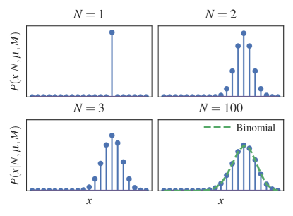
Figure 9: The marginal distribution of each individual covariate $x$ in the discrete microcanonical model, given by Eq. 77, approaches asymptotically the binomial distribution as the number of values $N$ increases, and the mean $\bar{x}=\mu/N$ is kept fixed.

The parameter $\mu$ is a non-negative integer that can be chosen arbitrarily, as long as the inequality $M\geq\mu/N$ is satisfied. Therefore, we may sample $\mu$ from the distribution of Eq. 67 in an unconstrained manner, and then sample the parameter $M$ from a constrained distribution $P(M|\mu,N)$. Incorporating this into the SBM yields,

$$P(\bm{x}|\bm{A},\bm{\mu}^{1},\bm{b}^{1})=\prod_{r\leq s}P(\bm{x}_{rs}^{1}|\mu_{rs}^{1},M),$$ (78)

and the overall marginal distribution

$$P(\bm{x},M|\bm{A},\{\bm{b}^{l}\}) =\sum_{\{\mu^{l}_{rs}\}}P(\bm{x}|\bm{A},\bm{\mu}^{1},\bm{b}^{1})P(M|\bm{\mu}^{1},\bm{A},\bm{b}^{1})\prod_{l=1}^{L}\prod_{r\leq s}\left[P(\bm{\mu}^{l}_{rs}|\mu^{l+1}_{b_{r}^{(l+1)},b_{s}^{(l+1)}})\right]^{1-\delta_{m_{rs}^{l},0}}$$ (79)

$$=P(M|\bar{\bm{\mu}}^{1},\bm{A},\bm{b}^{1})\left[\prod_{i\leq j}{M\choose x_{ij}}\right]\left[\prod_{r\leq s}{Mm_{rs}^{1}\choose\bar{\mu}_{rs}^{1}}^{-1}\right]\prod_{l=2}^{L}\prod_{r\leq s}\left[\left(\kern-3.00003pt\left(\genfrac{}{}{0.0pt}{}{m_{rs}^{l}}{\bar{\mu}_{rs}^{l}}\right)\kern-3.00003pt\right)^{-1}\right]^{1-\delta_{\bar{\mu}_{rs}^{l},0}},$$ (80)

where $P(M|\bar{\bm{\mu}}^{1},\bm{A},\bm{b}^{1})$ is a prior distribution for $M$ that respects the constraint $M\geq\bar{\mu}_{rs}^{1}/m_{rs}^{1}$. Thus, given any arbitrary value $M^{*}$, we can choose

$$P(M|\bar{\bm{\mu}}^{1},\bm{A},\bm{b}^{1})\\ =\begin{cases}1&\text{ if }M=\max\left(M^{*},{\lceil\max_{rs}\bar{\mu}^{1}_{rs}/m^{1}_{rs}\rceil}\right),\\ 0&\text{ otherwise,}\end{cases}$$ (81)

such that if $M^{*}$ is compatible with the observed covariates, i.e. $M^{*}\geq x_{ij}$, we have $P(M^{*}|\bar{\bm{\mu}}^{1},\bm{A},\bm{b}^{1})=1$ for any possible value of $\bar{\bm{\mu}}^{1}$ and $\bm{b}^{1}$ encountered in the posterior, as long as $M=M^{*}$, thereby effectively removing it from Eq. 80. A completely nonparametric approach would require us to include a prior $P(M^{*})$, but since it is a single global number, we can safely omit it, as it cannot influence the posterior distribution of partitions. In most practical scenarios, the bound $M^{*}$ is known a priori; otherwise it can be chosen as $M^{*}=\max_{ij}x_{ij}$.

IV.5 Poisson discrete weights

A natural extension of the binomial weights is the situation where $M\to\infty$ with the mean $\lambda=pM$ kept fixed, which yields the Poisson distribution

$$P(x|\lambda)=\frac{\lambda^{x}\mathrm{e}^{-\lambda}}{x!}.$$ (82)

Using this in the SBM gives us

$$P(\bm{x}|\bm{A},\bm{b},\bm{\lambda}) =\prod_{i<j}P(x_{ij}|\lambda_{b_{i},b_{j}})^{A_{ij}}$$ (83)

$$=\left[\prod_{i<j}x_{ij}!^{A_{ij}}\right]^{-1}\prod_{r\leq s}\lambda_{rs}^{\mu_{rs}}\mathrm{e}^{-m_{rs}\lambda_{rs}}.$$ (84)

Once more, the conjugate prior is the gamma distribution of Eq. 25, which after integrating over $\lambda_{rs}$ yields the marginal distribution

$$P(\bm{x}|\bm{A},\bm{b},\alpha,\beta)=\\ \left[\prod_{i<j}x_{ij}!^{A_{ij}}\right]^{-1}\prod_{r\leq s}\frac{\beta^{\alpha}\Gamma(\mu_{rs}+\alpha)}{\Gamma(\alpha)(m_{rs}+\beta)^{\mu_{rs}+\alpha}}.$$ (85)

The uninformative maximum entropy choice is $\alpha=1$, yielding

$$P(\bm{x}|\bm{A},\bm{b},\beta)=\left[\prod_{i<j}x_{ij}!^{A_{ij}}\right]^{-1}\prod_{r\leq s}\frac{\beta\mu_{rs}!}{(m_{rs}+\beta)^{\mu_{rs}+1}}.$$ (86)

But once more, we can obtain a deeper hierarchical model by formulating an asymptotically equivalent microcanonical model.

IV.5.1 Microcanonical distribution

The joint distribution of $N$ Poisson variables $\bm{x}=\{x_{1},\dots,x_{N}\}$ can be decomposed into a Poisson distribution for the total sum $\mu$ with mean $N\lambda$ and a uniform multinomial distribution for $\bm{x}$ conditioned on the total sum, i.e.

$$P(\bm{x}|\lambda)=P(\bm{x}|\mu)P(\mu|N\lambda).$$ (87)

The microcanonical version, therefore, is given simply by replacing $P(\mu|N\lambda)\to\delta_{\mu,\sum_{i}x_{i}}$, yielding

$$P(\bm{x}|\mu)=\frac{\mu!}{\prod_{i}x_{i}!}\frac{1}{N^{\mu}}\delta_{\mu,\sum_{i}x_{i}}.$$ (88)

The marginal distribution of the individual covariates $x_{i}$ can be obtained again as

$$P(x_{i}|N,\mu) =\frac{P(\bm{x}|\mu)}{P(\bm{x}\setminus x_{i}|\mu-x_{i})},$$ (89)

$$=\frac{\mu!(N-1)^{\mu-x_{i}}}{(\mu-x)!N^{\mu}x_{i}!},$$ (90)

The global constraint on the total sum has a vanishing effect for sufficiently large $N$, as long as the mean $\mu/N$ is kept fixed, as the marginal distribution of individual values $x_{i}$ will follow asymptotically a Poisson distribution with $\lambda=\mu/N$ (see Fig. 10).

The parameter $\mu$ is a non-negative integer that can be chosen arbitrarily. Therefore, we may sample $\mu$ from the distribution of Eq. 67. Incorporating this into the SBM yields,

$$P(\bm{x}|\bm{A},\bm{\mu}^{1},\bm{b}^{1})=\prod_{r\leq s}P(\bm{x}_{rs}^{1}|\mu_{rs}^{1}),$$ (91)

and the overall marginal distribution

$$P(\bm{x}|\bm{A},\{\bm{b}^{l}\}) =\sum_{\{\mu^{l}_{rs}\}}P(\bm{x}|\bm{A},\bm{\mu}^{1},\bm{b}^{1})\prod_{l=1}^{L}\prod_{r\leq s}\left[P(\bm{\mu}^{l}_{rs}|\mu^{l+1}_{b_{r}^{(l+1)},b_{s}^{(l+1)}})\right]^{1-\delta_{m_{rs}^{l},0}}$$ (92)

$$=\left[\prod_{i\leq j}x_{ij}!^{A_{ij}}\right]^{-1}\left[\prod_{r\leq s}\left(\frac{\bar{\mu}_{rs}^{1}!}{(m_{rs}^{1})^{\bar{\mu}_{rs}^{1}}}\right)^{1-\delta_{m_{rs}^{1},0}}\right]\prod_{l=2}^{L}\prod_{r\leq s}\left[\left(\kern-3.00003pt\left(\genfrac{}{}{0.0pt}{}{m_{rs}^{l}}{\bar{\mu}_{rs}^{l}}\right)\kern-3.00003pt\right)^{-1}\right]^{1-\delta_{\bar{\mu}_{rs}^{l},0}}.$$ (93)

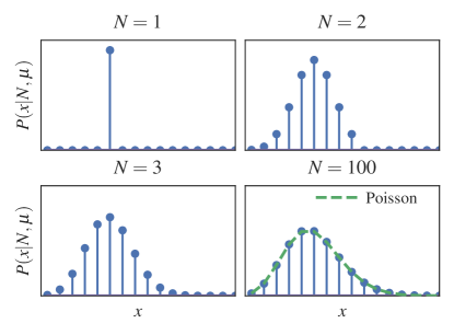
Figure 10: The marginal distribution of each individual covariate $x$ in the discrete microcanonical model, given by Eq. 90, approaches asymptotically the Poisson distribution as the number of values $N$ increases, and the mean $\bar{x}=\mu/N$ is kept fixed.

IV.6 Transformed weights

The models above can be easily modified to accommodate a much wider class of covariates, without any substantial change to the likelihoods, via variable transformations of the type $y_{ij}=f(x_{ij})$, according to some function $f(x)$. For the continuous models in particular, such variable transformations yield the scaled marginal likelihoods

$$P(\bm{x}|\bm{A},\{\bm{b}^{l}\})=P(\bm{y}(\bm{x})|\bm{A},\{\bm{b}^{l}\})\prod_{i<j}\left[\frac{\mathrm{d}f}{\mathrm{d}x}(x_{ij})\right]^{A_{ij}}.$$ (94)

The product of derivatives in the equation above is a multiplicative constant that does not depend on the hierarchical partition $\{\bm{b}^{l}\}$, and hence does not affect the posterior distribution (although it is relevant for model selection; see Sec. IV.7 below). We are thus free to choose any weight transformation $f(x)$, and use the previously defined distributions and associated algorithms on the transformed weights, without any other alteration. This gives us a wider class of covariate models that may be better suitable for specific datasets, and can be developed in an ad hoc manner. In the following, we cover some typical examples, non-exhaustively.

IV.6.1 Broadly distributed weights

If the observed weights are positive and broadly distributed, a possibly better model is the Pareto distribution,

$$P(x|\alpha,x_{m})=\begin{cases}\displaystyle\frac{\alpha x_{m}^{\alpha}}{x^{\alpha+1}},&\text{ if }x>x_{m},\\ 0,&\text{ otherwise.}\end{cases}$$ (95)

Instead of computing the integrated likelihood from scratch, we use the fact that the variable transformation $y=\ln(x/x_{m})$ yields

$$P(y|\alpha)=\alpha\mathrm{e}^{-\alpha y},$$ (96)

which is the exponential distribution we used before. So when dealing with broad weights, we can just make this transformation on the weights and use the exponential model.

Alternatively, we may use the normal model for $y=\ln x$, which assumes that $x$ is distributed according to a log-normal. In our experience, we found that this choice also typically yields better results when the positive weights are peaked around a typical value, in a manner that is difficult to represent with a mixture of exponential distributions.

IV.6.2 Bounded weights

If the weights are bounded in an interval $x\in[a,b]$, we can adapt it to an unbounded distribution by first uniformly mapping the weights to the unit interval $x^{\prime}\in[0,1]$, via

$$x^{\prime}=\frac{x-a}{b-a},$$ (97)

and then using a logit transformation

$$y=\ln\left(\frac{x^{\prime}}{1-x^{\prime}}\right),$$ (98)

or, equivalently, first mapping to the symmetric interval $x^{\prime}\in[-1,1]$, via

$$x^{\prime}=2\frac{x-a}{b-a}-1,$$ (99)

and using the inverse hyperbolic tangent

$$y=2\,\text{arctanh}(x^{\prime})=\ln\left(\frac{1+x^{\prime}}{1-x^{\prime}}\right),$$ (100)

both of which yield the same signed unbounded weight $y\in[-\infty,\infty]$, which can be fit using the normal distribution. Alternatively, the negative logarithm can be used with Eq. 97

$$z=-\ln x^{\prime},$$ (101)

which yields a positive unbounded weight $z\in[0,\infty]$ that can be used with the exponential distribution. Which approach is most suitable depends on the actual shape of the data, and can be determined a posteriori via model selection, as described in Sec. IV.7.

IV.6.3 Decomposing covariates

We can also obtain more elaborate models by decomposing a single covariate into multiple ones. Consider, for example, the case of signed discrete weights $x\in[\dots,-2,-1,0,1,2,\dots]$, which was not considered directly by any of the models so far. This can be done in a straightforward manner by decomposing the numbers into a sign and magnitude, i.e.

$$x_{ij}=(2s_{ij}-1)y_{ij}$$ (102)

where

$$s_{ij} =(\operatorname{sgn}(x_{ij})+1)/2,$$ (103)

$$y_{ij} =\operatorname{abs}(x_{ij})$$ (104)

is a reversible transformation that extracts the sign and absolute values of $x_{ij}$. We may then use a Binomial distribution with $M=1$ (i.e. Bernoulli) for $s_{ij}\in\{0,1\}$, and any non-negative distribution for $y_{ij}\in\{0,1,2,\dots\}$, and obtain the posterior using the joint marginal likelihood

$$P(\bm{x}|\bm{A},\{\bm{b}^{l}\}) =P(\bm{y},\bm{s}|\bm{A},\{\bm{b}^{l}\})$$ (105)

$$=P(\bm{y}|\bm{A},\{\bm{b}^{l}\})P(\bm{s}|\bm{A},\{\bm{b}^{l}\}).$$ (106)

IV.7 Model selection

Given any two models $\mathcal{M}_{1}$ and $\mathcal{M}_{2}$ for the same weighted network with edge covariates $\bm{x}$, for which we obtain the partitions $\{\bm{b}^{l}\}_{1}$ and $\{\bm{b}^{l}\}_{2}$ from their respective posterior distributions, we can perform model selection as described in Ref. Peixoto (2017b), by computing the posterior odds ratio

$$\Lambda =\frac{P(\{\bm{b}^{l}\}_{1},\mathcal{M}_{1}|\bm{A},\bm{x})}{P(\{\bm{b}^{l}\}_{2},\mathcal{M}_{2}|\bm{A},\bm{x})}$$ (107)

$$=\frac{P(\bm{A}|\{\bm{b}^{l}\}_{1},\mathcal{M}_{1})P(\bm{x}|\bm{A},\{\bm{b}^{l}\}_{1},\mathcal{M}_{1})P(\{\bm{b}^{l}\}_{1})P(\mathcal{M}_{1})}{P(\bm{A}|\{\bm{b}^{l}\}_{2},\mathcal{M}_{2})P(\bm{x}|\bm{A},\{\bm{b}^{l}\}_{2},\mathcal{M}_{2})P(\{\bm{b}^{l}\}_{2})P(\mathcal{M}_{2})},$$ (108)

where $P(\mathcal{M})$ is the prior preference for either model [typically, we are agnostic with $P(\mathcal{M}_{1})=P(\mathcal{M}_{2})$]. For values of $\Lambda>1$, the choice $(\{\bm{b}^{l}\}_{1},\mathcal{M}_{1})$ is preferred over $(\{\bm{b}^{l}\}_{2},\mathcal{M}_{2})$ according to the data, and the magnitude of $\Lambda$ yields the degree of statistical significance.

Using this criterion we can select between unweighted variations of the SBM (e.g. degree-corrected or not) Peixoto (2017b), but also between different models of the weights. This is particularly useful when using weight transformations as described in Sec. IV.6. For example, when considering two different transformations $y_{ij}=f(x_{ij})$ and $z_{ij}=g(x_{ij})$, using different models $\mathcal{M}_{y}$ and $\mathcal{M}_{z}$ for the transformed covariates, the posterior odds ratio [with agnostic priors $P(\mathcal{M}_{y})=P(\mathcal{M}_{z})$] becomes

$$\Lambda=\frac{P(\bm{A},\bm{y}(\bm{x})|\bm{A},\{\bm{b}^{l}\}_{1},\mathcal{M}_{y})P(\{\bm{b}^{l}\}_{1})\prod_{i<j}f^{\prime}(x_{ij})^{A_{ij}}}{P(\bm{A},\bm{z}(\bm{x})|\bm{A},\{\bm{b}^{l}\}_{2},\mathcal{M}_{z})P(\{\bm{b}^{l}\}_{2})\prod_{i<j}g^{\prime}(x_{ij})^{A_{ij}}}.$$ (109)

The approach is entirely analogous for transformations on discrete weights, where one simple omits the derivative terms.

Transformation	Derivatives	Weight model	$\ln P(\bm{A},\bm{x},\{\bm{b}^{l}\})$
$y_{ij}=x_{ij}$	$1$	Exponential	$-56,512$
$y_{ij}=\ln x_{ij}$	$\prod_{i<j}1/x_{ij}^{A_{ij}}$	Normal	$-52,054$

Table 1: Joint log-likelihood $\ln P(\bm{A},\bm{x},\{\bm{b}^{l}\})$ for the human brain data in Sec. III.3 using the electrical connectivity as edge covariate, for two model variations according to weight transformations.

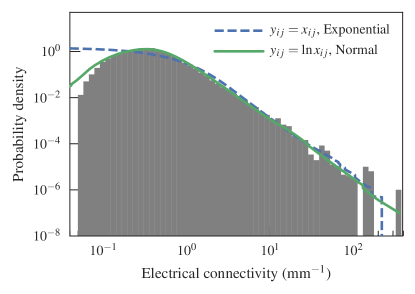
Figure 11: Overall distribution of the electrical connectivity of the human brain data. The solid lines shows the inferred distribution according to the weighted SBM using two models for the edge covariates, as shown in the legend.

We illustrate the use of this criterion on the human brain data analyzed in Sec. III.3. We consider here only the electric connectivity covariate, which is non-negative and unbounded in the range $[0,\infty]$. We consider two models for the weights: The first is the exponential model of Sec. IV.1 applied directly to the original covariates, and the second is the normal model of Sec. IV.2, applied to the transformed weights $y_{ij}=\ln x_{ij}$, which results in a log-normal model for $x_{ij}$. As the results of Table 1 show, we obtain for this dataset a posterior odds ratio of $\ln\Lambda\approx 4,458$ favoring the log-normal model, despite the fact that it contains more internal parameters. As we see in Fig. 11, indeed the log-normal model is better suited to capture the peaked nature of the overall distribution. It should be noted that while it is a trivial feat to obtain better fits with more complicated models, the Bayesian criterion above takes into account the complexity of the model, and will point towards a more complicated one only if the statistical evidence in the data supports it.

V Conclusion

The weighted extensions of the SBM presented in this work allow for a principled inference of large-scale modular structure of weighted networks, in a manner that is fully nonparametric, and algorithmically efficient. As they include a hierarchical description of the network — taking into account both the node adjacency as well as the edge weights — our SBM implementations enable the detection of modular structures at multiple scales, without being biased towards any specific kind of mixing pattern (such as assortativity) in any of them.

The nonparametric nature of our approach means that it can be used to detect the most appropriate model dimension, including the number of groups as well as size and shape of the hierarchical division, directly from data, in a parsimonious way, without requiring any prior input. This comes with the guarantee that the inferred hierarchy is statistically significant, and hence is not the result of statistical fluctuations of a simpler model (such as a completely random graph).

The edge weights are included in the model description as additional covariates, and thus require specific models that reflect their nature. The explicit variations presented in this work cover a broad range of possible types of covariates, that can be either continuous or discrete, signed or unsigned, bounded or unbounded. Furthermore, all these particular variations can be arbitrarily extended to accommodate a much wider class of weight models via variable transformations, which incur no modification to the algorithms. Such transformations can be performed in an ad hoc manner, reflecting the specificity of the data at hand, and the best choice can be evaluated a posteriori using Bayesian model selection, simultaneously taking into account the quality of fit, the model complexity and the statistical evidence available from the data.

Although we do not describe this in detail here, it is easy to see that the exact same approach we present can be used for other variations of the SBM, such as with overlapping groups Ball et al. (2011); Peixoto (2015a), edge layers Peixoto (2015b); Stanley et al. (2016); Heimlicher et al. (2012) and dynamic networks Xu and Iii (2013); Peixoto (2015b); Peixoto and Rosvall (2017).

Despite its advantages, our approach inherits the limitations of the underlying SBM ansatz. In particular, it assumes that the weights are distributed on the edges in a manner that is (asymptotically, in the microcanonical case) conditionally independent. Hence, in the same manner that the unweighted SBM does not include the often realistic propensity of the network to form triangles and other local structures, the weighted extensions preclude the existence of certain kinds of weight correlations that are known to exist in key cases MacMahon and Garlaschelli (2015). The development of tractable and versatile models that incorporate such higher-order aspects remains an open challenge.

Appendix A Directed networks

Although we focused on undirected networks in the main text, our methods can be easily adapted to directed networks. The models for directed adjacency matrices $P(\bm{A}|\{\bm{b}^{l}\})$ are described in detail in Ref Peixoto (2017b). For the edge covariates, the modifications are straightforward yielding expressions for $P(\bm{x}|\bm{A},\{\bm{b}^{l}\})$ that are identical, but with products going over directed pairs of groups and nodes, i.e. $\prod_{r\leq s}\to\prod_{rs}$ and $\prod_{i\leq j}\to\prod_{ij}$. Our reference implementation supports these variations Peixoto (2014c).

References

- Fortunato (2010) Santo Fortunato, “Community detection in graphs,” Physics Reports 486, 75–174 (2010).
- Peixoto (2017a) Tiago P. Peixoto, “Bayesian stochastic blockmodeling,” arXiv:1705.10225 [cond-mat, physics:physics, stat] (2017a), arXiv: 1705.10225.
- Holland et al. (1983) Paul W. Holland, Kathryn Blackmond Laskey, and Samuel Leinhardt, “Stochastic blockmodels: First steps,” Social Networks 5, 109–137 (1983).
- Aicher et al. (2015) Christopher Aicher, Abigail Z. Jacobs, and Aaron Clauset, “Learning latent block structure in weighted networks,” Journal of Complex Networks 3, 221–248 (2015).
- Peixoto (2014a) Tiago P. Peixoto, “Hierarchical Block Structures and High-Resolution Model Selection in Large Networks,” Physical Review X 4, 011047 (2014a).
- Peixoto (2017b) Tiago P. Peixoto, “Nonparametric Bayesian inference of the microcanonical stochastic block model,” Physical Review E 95, 012317 (2017b).
- Peixoto (2013) Tiago P. Peixoto, “Parsimonious Module Inference in Large Networks,” Physical Review Letters 110, 148701 (2013).
- Karrer and Newman (2011) Brian Karrer and M. E. J. Newman, “Stochastic blockmodels and community structure in networks,” Physical Review E 83, 016107 (2011).
- Guimerà and Sales-Pardo (2009) Roger Guimerà and Marta Sales-Pardo, “Missing and spurious interactions and the reconstruction of complex networks,” Proceedings of the National Academy of Sciences 106, 22073 –22078 (2009).
- Yan et al. (2010) Xiaoran Yan, Yaojia Zhu, Jean-Baptiste Rouquier, and Cristopher Moore, “Active Learning for Hidden Attributes in Networks,” arXiv:1005.0794 (2010).
- Côme and Latouche (2015) Etienne Côme and Pierre Latouche, “Model selection and clustering in stochastic block models based on the exact integrated complete data likelihood,” Statistical Modelling 15, 564–589 (2015).
- Newman and Reinert (2016) M. E. J. Newman and Gesine Reinert, “Estimating the Number of Communities in a Network,” Physical Review Letters 117, 078301 (2016).
- Jaynes (2003) E. T. Jaynes, Probability Theory: The Logic of Science, edited by G. Larry Bretthorst (Cambridge University Press, Cambridge, UK ; New York, NY, 2003).
- Metropolis et al. (1953) Nicholas Metropolis, Arianna W. Rosenbluth, Marshall N. Rosenbluth, Augusta H. Teller, and Edward Teller, “Equation of State Calculations by Fast Computing Machines,” The Journal of Chemical Physics 21, 1087 (1953).
- Hastings (1970) W. K. Hastings, “Monte Carlo sampling methods using Markov chains and their applications,” Biometrika 57, 97 –109 (1970).
- Peixoto (2014b) Tiago P. Peixoto, “Efficient Monte Carlo and greedy heuristic for the inference of stochastic block models,” Physical Review E 89, 012804 (2014b).
- Peixoto (2014c) Tiago P. Peixoto, “The graph-tool python library,” figshare (2014c), 10.6084/m9.figshare.1164194, available at https://graph-tool.skewed.de.
- Holten (2006) D. Holten, “Hierarchical Edge Bundles: Visualization of Adjacency Relations in Hierarchical Data,” IEEE Transactions on Visualization and Computer Graphics 12, 741–748 (2006).
- Note (1) Data available at https://www.un.org/en/development/desa/population/migration/data/estimates2/estimates15.shtml.
- Note (2) Data available from the official website http://www2.camara.leg.br/.
- Szalkai et al. (2017) Balázs Szalkai, Csaba Kerepesi, Bálint Varga, and Vince Grolmusz, “Parameterizable consensus connectomes from the Human Connectome Project: the Budapest Reference Connectome Server v3.0,” Cognitive Neurodynamics 11, 113–116 (2017).
- McNab et al. (2013) Jennifer A. McNab, Brian L. Edlow, Thomas Witzel, Susie Y. Huang, Himanshu Bhat, Keith Heberlein, Thorsten Feiweier, Kecheng Liu, Boris Keil, Julien Cohen-Adad, M. Dylan Tisdall, Rebecca D. Folkerth, Hannah C. Kinney, and Lawrence L. Wald, “The Human Connectome Project and beyond: Initial applications of 300mt/m gradients,” NeuroImage Mapping the Connectome, 80, 234–245 (2013).
- Basser and Pierpaoli (1996) Peter J. Basser and Carlo Pierpaoli, “Microstructural and physiological features of tissues elucidated by quantitative-diffusion-tensor MRI,” Journal of Magnetic Resonance Magnetic Moments, 213, 560–570 (1996).
- Meunier et al. (2010) David Meunier, Renaud Lambiotte, and Edward T. Bullmore, “Modular and Hierarchically Modular Organization of Brain Networks,” Frontiers in Neuroscience 4 (2010), 10.3389/fnins.2010.00200.
- Bassett et al. (2013) Danielle S. Bassett, Mason A. Porter, Nicholas F. Wymbs, Scott T. Grafton, Jean M. Carlson, and Peter J. Mucha, “Robust detection of dynamic community structure in networks,” Chaos: An Interdisciplinary Journal of Nonlinear Science 23, 013142 (2013).
- Betzel et al. (2013) Richard F. Betzel, Alessandra Griffa, Andrea Avena-Koenigsberger, Joaquín Goñi, Jean-Philippe Thiran, Patric Hagmann, and Olaf Sporns, “Multi-scale community organization of the human structural connectome and its relationship with resting-state functional connectivity,” Network Science 1, 353–373 (2013).
- Newman (2003) M. E. J. Newman, “Mixing patterns in networks,” Phys. Rev. E 67, 026126 (2003).
- Girvan and Newman (2002) M. Girvan and M. E. J. Newman, “Community structure in social and biological networks,” Proceedings of the National Academy of Sciences 99, 7821 –7826 (2002).
- Guimerà et al. (2004) Roger Guimerà, Marta Sales-Pardo, and Luís A. Nunes Amaral, “Modularity from fluctuations in random graphs and complex networks,” Physical Review E 70, 025101 (2004).
- Reichardt and Bornholdt (2006) Jörg Reichardt and Stefan Bornholdt, “When are networks truly modular?” Physica D: Nonlinear Phenomena 224, 20–26 (2006).
- Bagrow (2012) James P. Bagrow, “Communities and bottlenecks: Trees and treelike networks have high modularity,” Physical Review E 85, 066118 (2012).
- McDiarmid and Skerman (2013) Colin McDiarmid and Fiona Skerman, “Modularity in random regular graphs and lattices,” Electronic Notes in Discrete Mathematics 43, 431–437 (2013).
- McDiarmid and Skerman (2016) Colin McDiarmid and Fiona Skerman, “Modularity of tree-like and random regular graphs,” ArXiv e-prints 1606, arXiv:1606.09101 (2016).
- Prokhorenkova et al. (2016) Liudmila Ostroumova Prokhorenkova, Paweł Prałat, and Andrei Raigorodskii, “Modularity of Complex Networks Models,” in Algorithms and Models for the Web Graph, Lecture Notes in Computer Science (Springer, Cham, 2016) pp. 115–126.
- Fortunato and Barthélemy (2007) Santo Fortunato and Marc Barthélemy, “Resolution limit in community detection,” Proceedings of the National Academy of Sciences 104, 36–41 (2007).
- Fortunato and Hric (2016) Santo Fortunato and Darko Hric, “Community detection in networks: A user guide,” Physics Reports (2016), 10.1016/j.physrep.2016.09.002.
- Betzel et al. (2017) Richard F. Betzel, John D. Medaglia, and Danielle S. Bassett, “Diversity of meso-scale architecture in human and non-human connectomes,” ArXiv e-prints 1702, arXiv:1702.02807 (2017).
- Box and Tiao (2011) George E. P. Box and George C. Tiao, Bayesian Inference in Statistical Analysis (John Wiley & Sons, 2011) google-Books-ID: T8Askeyk1k4C.
- Godoy-Lorite et al. (2016) Antonia Godoy-Lorite, Roger Guimerà, Cristopher Moore, and Marta Sales-Pardo, “Accurate and scalable social recommendation using mixed-membership stochastic block models,” Proceedings of the National Academy of Sciences 113, 14207–14212 (2016).
- Ball et al. (2011) Brian Ball, Brian Karrer, and M. E. J. Newman, “Efficient and principled method for detecting communities in networks,” Physical Review E 84, 036103 (2011).
- Peixoto (2015a) Tiago P. Peixoto, “Model Selection and Hypothesis Testing for Large-Scale Network Models with Overlapping Groups,” Physical Review X 5, 011033 (2015a).
- Peixoto (2015b) Tiago P. Peixoto, “Inferring the mesoscale structure of layered, edge-valued, and time-varying networks,” Physical Review E 92, 042807 (2015b).
- Stanley et al. (2016) N. Stanley, S. Shai, D. Taylor, and P. J. Mucha, “Clustering Network Layers with the Strata Multilayer Stochastic Block Model,” IEEE Transactions on Network Science and Engineering 3, 95–105 (2016).
- Heimlicher et al. (2012) Simon Heimlicher, Marc Lelarge, and Laurent Massoulié, “Community Detection in the Labelled Stochastic Block Model,” arXiv:1209.2910 (2012).
- Xu and Iii (2013) Kevin S. Xu and Alfred O. Hero Iii, “Dynamic Stochastic Blockmodels: Statistical Models for Time-Evolving Networks,” in Social Computing, Behavioral-Cultural Modeling and Prediction, Lecture Notes in Computer Science No. 7812, edited by Ariel M. Greenberg, William G. Kennedy, and Nathan D. Bos (Springer Berlin Heidelberg, 2013) pp. 201–210.
- Peixoto and Rosvall (2017) Tiago P. Peixoto and Martin Rosvall, “Modelling sequences and temporal networks with dynamic community structures,” Nature Communications 8, 582 (2017).
- MacMahon and Garlaschelli (2015) Mel MacMahon and Diego Garlaschelli, “Community Detection for Correlation Matrices,” Physical Review X 5, 021006 (2015).