The ESO Diffuse Interstellar Bands Large Exploration Survey

The carriers of the diffuse interstellar bands (DIBs) are largely unidentified molecules ubiquitously present in the interstellar medium (ISM). After decades of study, two strong and possibly three weak near-infrared DIBs have recently been attributed to the C${}_{60}^{+}$ fullerene based on observational and laboratory measurements. There is great promise for the identification of the over 400 other known DIBs, as this result could provide chemical hints towards other possible carriers.

In an effort to systematically study the properties of the DIB carriers, we have initiated a new large-scale observational survey: the ESO Diffuse Interstellar Bands Large Exploration Survey (EDIBLES). The main objective is to build on and extend existing DIB surveys to make a major step forward in characterising the physical and chemical conditions for a statistically significant sample of interstellar lines-of-sight, with the goal to reverse-engineer key molecular properties of the DIB carriers.

EDIBLES is a filler Large Programme using the Ultraviolet and Visual Echelle Spectrograph at the Very Large Telescope at Paranal, Chile. It is designed to provide an observationally unbiased view of the presence and behaviour of the DIBs towards early-spectral-type stars whose lines-of-sight probe the diffuse-to-translucent ISM. Such a complete dataset will provide a deep census of the atomic and molecular content, physical conditions, chemical abundances and elemental depletion levels for each sightline. Achieving these goals requires a homogeneous set of high-quality data in terms of resolution ($R\sim 70\,000$ – $100\,000$), sensitivity (S/N up to 1000 per resolution element), and spectral coverage (305–1042 nm), as well as a large sample size (100$+$ sightlines). In this first paper the goals, objectives and methodology of the EDIBLES programme are described and an initial assessment of the data is provided.

1 Introduction

The unknown identity of the carriers of all but two diffuse interstellar bands (DIBs) constitutes the longest standing spectroscopic enigma of modern astronomy (Sarre 2006). Two features at 5797 and 5780 Å, which are now known to be interstellar in origin, were first noted by Heger (1922) and studied in relation to interstellar gas and dust by Merrill & Wilson (1938). At present, over 400 of these interstellar absorption features are known (for a handful of sightlines), superimposed on an otherwise nearly smooth interstellar extinction curve (Herbig 1995; Galazutdinov et al. 2000; Hobbs et al. 2008). Only recently has the attribution of a pair of near-infrared DIBs (Foing & Ehrenfreund 1994) to C${}_{60}^{+}$ been confirmed with laboratory gas phase experiments (Campbell et al. 2015; Kuhn et al. 2016) along with the tentative astronomical detection of three more predicted bands (Walker et al. 2015, 2016), though this needs further verification and investigation (Galazutdinov et al. 2017; Cordiner et al. 2017). This is an exciting result because C₆₀ (Cami et al. 2010; Sellgren et al. 2010), and C${}_{60}^{+}$ (Berné et al. 2013) have also recently been detected in space through their mid-infrared emission spectra. This identification may be a chemical clue towards identifying further DIB carriers; so far only C₃ (Haffner & Meyer 1995; Maier et al. 2001; Schmidt et al. 2014) and C${}_{60}^{+}$ have been identified as pure polyatomic carbon species in the diffuse ISM and this leaves a large gap to be filled in our current understanding of the carbon chemical network in diffuse clouds. It is possible that the detection of C${}_{60}^{+}$ hints at a long predicted important role of polycyclic aromatic hydrocarbons (PAHs) in the ISM (Van der Zwet & Allamandola 1985; Léger & d’Hendecourt 1985; Salama et al. 1996). Recent laboratory (Zhen et al. 2014) and modelling (Berné et al. 2015) works support the proposal by Berné & Tielens (2012) that fullerenes may form upon photo-dissociation of large PAH precursors.

Observational surveys (e.g. Herbig 1993; Friedman et al. 2011; Kos & Zwitter 2013) have shown that the strength of the strongest $\sim$20 of the DIBs correlates roughly linearly with the amount of dust and gas, measured by the reddening ${E}{\mathrm{(}B-V)}$ or the column density of atomic hydrogen $N$(H i), respectively. This indicates a thorough mixing of the DIB carriers with interstellar matter (Cox 2011). However, a large real scatter is observed in these relations with gas and dust, and the relative strengths of several bands are known to have an environmental dependence (Cox & Spaans 2006); some bands vary as a function of radiation strength between different lines-of-sight (Krełowski & Walker 1987; Cami et al. 1997; Vos et al. 2011; Friedman et al. 2011). The scatter is also partly due to multiple cloud structures along sightlines. The relationship between several DIBs and, for example, C₂ and CN, has been investigated (Thorburn et al. 2003; Weselak et al. 2008), but generally the link with di-atomic species is not well understood. This relation between DIBs and reddening has not been investigated for the remaining $>$380 bands. Whether or not there is a direct physical connection between DIB carriers and dust grains, e.g. in terms of depletion onto grains or as carrier formation sites, remains to be seen – so far no polarisation signal has been detected for the twenty strongest DIBs (Cox et al. 2011).

Studies of selected bands in a dozen sightlines have revealed a complex substructure in the narrowest bands (Sarre et al. 1995; Ehrenfreund & Foing 1996; Galazutdinov et al. 2008) which show small variations with local temperature (Cami et al. 2004; Kaźmierczak et al. 2010a), typical for a molecular carrier. Substructure has also been identified in weak DIBs, but line-of-sight variations are less well studied (Galazutdinov et al. 2005). On the other hand, broader DIBs do not contain substructure (Snow 2002; Galazutdinov et al. 2008), which may be due to lifetime broadening of the absorption band (Linnartz et al. 2010). Considerations of the available elemental abundances and plausible oscillator strengths lead to the conclusion that abundant large organic molecules are suitable candidates (Léger & d’Hendecourt 1985; Huang & Oka 2015). The combination of observational studies, theoretical models, and laboratory astrophysics indicates that candidate carriers should primarily be sought among a large number of possible carbon-based organic molecules [see Sarre (2006) for a review, and Cami & Cox (2014) for an overview of recent progress].

Ongoing and future large spectroscopic surveys offer the possibility to study (mostly the strongest) DIBs in large areas of the sky. For example, Lan et al. (2014) and Baron et al. (2015) constructed DIB strength maps from SDSS spectra, Kos et al. (2014) produced pseudo-3D maps for the 8621 Å DIB using the RAVE survey, Zasowski et al. (2015) and Elyajouri et al. (2016) used the APOGEE near-infrared survey to study the distribution of the 15267 Å near-infrared DIB. The spatial distribution and properties of DIBs can also be studied in smaller fields-of-view (van Loon et al. 2009; Raimond et al. 2012; Puspitarini et al. 2015) or closer regions, such as the Local Bubble (Farhang et al. 2015; Bailey et al. 2016).

In the last decade it has also been firmly established that many band carriers are universal; DIBs have been detected and surveyed in the Magellanic Clouds (Cox et al. 2006, 2007; Welty et al. 2006; van Loon et al. 2013; Bailey et al. 2015), in M31 and M33 (Cordiner et al. 2008, 2011), and in individual sightlines in more distant galaxies (Junkkarinen et al. 2004; Sollerman et al. 2005; Lawton et al. 2008; Cox & Patat 2008, 2014; Monreal-Ibero et al. 2015). DIB carriers therefore constitute an important reservoir of (organic) material throughout the Universe.

Identifying the DIB carriers and understanding their properties must come from high-quality data in the nearby Galactic interstellar medium (ISM). Identification of the carrier species will directly impact our understanding of interstellar chemistry, and can help reconstruct 3D line-of-sight properties if related to specific environments. It is clear that the ultimate confirmation must come from a direct comparison between astronomical, theoretical, and laboratory spectra over a broad wavelength range. A commonly applied and straightforward approach is to acquire laboratory spectra of possible candidate carriers taken under astrophysical relevant conditions until an unambiguous match with the astronomical data is found. With the notable exception of the above mentioned work on C${}_{60}^{+}$ previous studies have thus far failed, such as attempts to link PAH cations (Bréchignac & Pino 1999; Salama et al. 2011, 1999; Romanini et al. 1999), neutral PAHs (Salama et al. 2011; Gredel et al. 2011), carbon chains (Motylewski et al. 2000; Maier et al. 2004), or H₂ (Sorokin & Glownia 1999; Ubachs 2014) to the DIBs. The search for a laboratory match can be optimised if the most likely candidates can be pre-selected out of the vast collection of possible species, and if the relevant conditions can be accurately constrained. Hence it is necessary to unravel the physical and chemical properties of the DIB carriers through analysis and modelling of observations. This includes deriving environmental conditions that affect their strength/profile shapes, as well as understanding the molecular physics and spectroscopy of candidate carriers.

This paper presents the observational overview of the ESO Diffuse Interstellar Bands Large Exploration Survey (EDIBLES) and how we intend to use the obtained spectra in our long-term goal of reverse-engineering the molecular characteristics of DIB carriers. In Sect. 2 we describe the scientific goals and immediate objectives of EDIBLES. Sect. 3 describes the methodology and survey design. The survey target selection is discussed in Sect. 4 and the data processing steps are described in Sect. 5. Sect. 6 discusses several confounding factors such as telluric and stellar spectral lines. In Sect. 7 we present a preview of the EDIBLES data and illustrate their scope and quality. A brief summary is given in Sect. 8.

Table 1: UVES instrument setups used. The two spectrograph arms are used to collect data for a pair of wavelength regions simultaneously. A second setup allows the gaps to be covered with another pair of settings. For each setting we give the slit width, nominal resolving power, and nominal wavelengths covered. Red-L and Red-U refer to the spectra recorded with the Red Lower EEV CCD and the Red Upper MIT CCD (c.f. Sect. 5).

Setting	Arm	Slit width	Resolving	Spectral range
(nm)		(″)	power	(nm)
346	blue	0.4	71 000	304.2 – 387.2
564	red-L	0.3	107 000	461.6 – 560.8
	red-U			566.9 – 665.3
437	blue	0.4	71 000	375.2 – 498.8
860	red-L	0.3	107 000	670.4 – 853.9
	red-U			866.0 – 1042.0

2 Scientific goals & immediate objectives

The primary science goal of EDIBLES is to reverse-engineer molecular characteristics of DIB carriers, through studying the behaviour of DIBs in relation to the physical and chemical parameters of their environment. This approach differs from earlier work in which attempts to identify DIBs were based mainly on direct comparisons of astronomical and laboratory or theoretical spectra. A large systematic high-fidelity survey of the diffuse-to-translucent ISM is necessary to realise this approach.

The aim is to assemble a sample of interstellar spectra with sufficiently high spectral resolution and signal-to-noise ratio to allow detailed analysis of numerous DIBs and known atomic and molecular absorption lines in the same lines-of-sight. At the same time, our sample is designed to sample a wide range of interstellar conditions, in terms of reddening, molecular content and radiation field, within a practical observing time.

With EDIBLES we plan to compile the global properties of a large ensemble of both weak and strong DIBs, and variations therein, as a function of depletion (patterns) and local physical conditions. The new dataset should allow us to: (a) determine the relation between weak and strong DIBs by identifying correlations and sequences; (b) identify (sets of) DIBs that correlate with different physical conditions in the ISM, and assess whether the DIBs can be used to determine those conditions as a remote diagnostic tool; (c) study the physico-chemical parameters that influence the DIB properties, by using state-of-the-art chemical modelling, combined with extensive auxiliary line-of-sight data (e.g. on dust); and (d) constrain the chemical composition of the DIB carriers by studying their relation to interstellar elemental abundances (depletion levels) and dust grain properties and composition derived from, for example, the UV-visual extinction (including the conspicuous 2175 Å UV bump) and optical polarisation curves.

A number of studies have attempted to investigate links between the physical and chemical conditions of the ISM and the properties of the DIBs. However, most studies focus only on a few strong bands in a moderate-to-large number ($\approx$100) of sightlines (Friedman et al. 2011; Vos et al. 2011; Zasowski et al. 2015), or on many DIBs in just a few sightlines (Cami et al. 1997; Tuairisg et al. 2000; Hobbs et al. 2008, 2009). Hence, more recent progress in the field has been limited to the study of only a handful of the strongest DIBs due to high demands on the signal-to noise ratio (S/N), spectral resolution, the removal of stellar and telluric lines, and the lack of large, uniform data sets. EDIBLES is designed to fill this gap, making just such a large, uniform data set available and thus enabling a large and systematic study of the physical and chemical parameters that are expected to directly influence the formation efficiency and spectroscopic response of DIB carriers.

3 Methodology & survey design

EDIBLES provides the community with optical ($\sim$305–1042 nm) spectra at high spectral resolution (R $\sim$ 70 000 in the blue arm and 100 000 in the red arm) and high signal-to-noise (S/N; median value $\sim$ 500–1000), for a statistically significant sample of interstellar sightlines. Many of the $>$100 sightlines included in the survey already have auxiliary available ultraviolet, infrared and/or polarisation data on the dust and gas components.

Studies of DIBs typically report data such as equivalent width, central depth, profile shape and substructure identification. These cannot easily be compared between surveys due to differences in the instrumentation, data quality and analysis procedures – e.g. continuum normalisation and measurement of spectroscopic lines. Archival material comprises a heterogeneous sample of spectra with varying S/N, resolving power, and spectral coverage. To achieve the goals and objectives described above requires a large and homogeneous survey of UV/visible spectroscopic tracers across a broad spectral range, covering a broad variety of interstellar environments. From this self-consistent set of observations we can extract:

1. Accurate column density measurements (or upper limits) for the most important atomic and molecular species, across a wide spectral range. These can be used to assess the velocity structure of the line-of-sight (in particular to determine radial velocity differences between species; e.g. Bondar et al. 2007), derive depletion levels of metals, infer and compute physical conditions (within the limitations imposed by the current knowledge on interstellar processes), using diffuse cloud PDR models (Le Petit et al. 2006) or turbulent energy dissipation models (c.f. Flower & Pineau des Forêts 2015; Godard et al. 2014; Bron 2014).

   For the photo-chemistry and derivation of particle density, radiation fields, turbulent energy dissipation, the key transitions are those of CN $\lambda\lambda$3874, 7906, CH $\lambda\lambda$3879, 4300, and CH⁺ $\lambda\lambda$3958, 4232 Å, together with H₂ (from archival UV spectroscopy). For example, rotational temperatures can be derived from bands of C₂ ($\lambda 8756$) and C₃ ($\lambda$4053), and cosmic ray ionisation rates can be derived from OH⁺ abundances ($\lambda\lambda$3300–3600 Å). CH measurements can be used to estimate the H₂ column density (Danks et al. 1984; Weselak et al. 2004).

2. Accurate measurements of DIB profiles (asymmetries, wings, substructure) and variations therein. Substructure can be related to molecular properties / sizes of carrier species (Kerr et al. 1996; Ehrenfreund & Foing 1996; Huang & Oka 2015) with variations due to changes in the rotational temperature (Cami et al. 2004; Kaźmierczak et al. 2010b) or the presence of hot bands (Marshall et al. 2015).

3. Updated measurements of peak positions of weak (per unit reddening) diffuse bands along single cloud sightlines.

4. Measurements and cross-correlation of over 50 weak and strong bands along the most reddened sightlines (${E}{\mathrm{(}B-V)}$ $>$ 0.4 mag). Correlations between strong and weak bands might reveal additional information on groups (or families) of DIBs, but it should be noted that a strong correlation between DIBs is not a necessarily a guarantee that they have a common carrier (McCall et al. 2010; Krełowski et al. 2016).

5. Stacking analyses to search for molecules and/or DIBs which are too weak to be seen in individual spectra.

6. Firm detection limits or abundance constraints on specific molecular carriers for which laboratory spectra are obtained.

7. Variations in interstellar species due to the small-scale structure of the diffuse ISM (Cordiner et al. 2013; Smith et al. 2013).

Figure 1: Galactic distribution of EDIBLES targets. The symbol size reflects the value of $R_{V}$, while the interior colour represents the line-of-sight reddening, ${E}{\mathrm{(}B-V)}$. Symbols with green edges represent the observed targets, while blue edges correspond to the targets to be observed by the end of the programme.

To achieve our objectives efficiently we use the Ultra-violet Visual Echelle Spectrograph (UVES; Dekker et al. 2000; Smoker et al. 2009) mounted on the 8-metre second Unit Telescope (UT2) of the ESO (European Southern Observatory) Very Large Telescope at the Paranal Observatory. The relative brightness of nearby early-type stars allows the observation strategy to take advantage of poor observing conditions and twilight hours that would otherwise be under-utilised. The programme is running as a Large ‘Filler’ Programme (ESO ID 194.C-0833, PI. N.L.J. Cox), which has been allocated 280 hours of observing time. About 8 500 science exposures with a total exposure time of 229 hours (with blue and red arm exposures taken simultaneously) have been collected between September 2014 and May 2017. The program is expected to be completed by late 2017.

UVES has two arms, red and blue, which can be used simultaneously by inserting a dichroic mirror (Dekker et al., 2000). To obtain coverage of the entire spectral range accessible with UVES, we use two instrumental settings per target: setting #1: 346+564 and setting #2: 437+860, where the pairs of numbers refer to the central wavelengths in nanometres of the two arms. Together this provides near-continuous wavelength coverage from $\sim$305 to 1042 nm. The blue and red arm slit widths are 0.4″ and 0.3″, respectively, yielding nominal resolving powers $R=\lambda/\Delta\lambda$ of $\sim$71 000 and $\sim$107 000. Table 1 presents a summary of the instrumental setups. The EDIBLES data presented here were collected over a period of two years, and it is therefore important to realize that the UVES resolution is not fully stable with time, but the values listed in Table 1 were typically realised in the actual spectra.

The “filler”-type observation strategy means that observations are often executed in non-optimal (and unpredictable) conditions e.g. in terms of seeing, cloud coverage, sky emission/air glow, lunar phase, and water vapour content. This needs to be taken into account in the implementation of the observations. Despite these limitations, S/N ratios of 200–300 per exposure can be reached in short exposure times for the bright ($2<V<6$ mag) targets, and up to 20 exposures (to avoid saturation of individual frames) are obtained for each to build up higher S/N. Observations are divided into observing blocks (OBs) for a specific instrument setting and target. OB execution times range from $\sim$20 minutes for the bright ($V<6$ mag) stars up to $\sim$45 minutes for the fainter ($6<V<9$) stars.

Additional flat-field calibration exposures were taken during the day-time (when possible, subject to operational constraints) to reduce residual fringing that would persist with the standard UVES calibration plan and to increase the overall S/N ratio. Details of the flat-field corrections are given in Sect. 5.

Figure 2: Number of selected targets as function of reddening ${E}{\mathrm{(}B-V)}$, extinction $A_{V}$, the ratio of total-to-selective extinction $R_{V}$ ($=A_{V}$/${E}{\mathrm{(}B-V)}$), and the fraction of molecular hydrogen $f_{\text{H}_{2}}$for the target sample. The number of observed targets with reported values for each quantity are given at the top of each panel. The dark blue and light blue distributions correspond to the samples of observed and observed $+$ foreseen targets. The vertical red lines indicate the value of the 5, 10, 25, 50, 75, 90, and 95 percentiles of each sample. The labels are located such that they trace the cumulative target distribution.

4 Target survey sample selection and characteristics

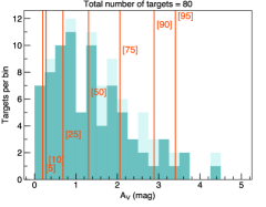
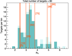
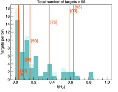
We constructed a statistically representative survey sample that probes a wide range of interstellar environment parameters including reddening ${E}{\mathrm{(}B-V)}$, visual extinction $A_{V}$, total-to-selective extinction ratio $R_{V}$, and molecular hydrogen fraction $f_{\text{H}_{2}}$. This is essential to (a) trace depletion patterns from diffuse $\rightarrow$ translucent clouds, (b) study the effect of shock- and photo-processing, (c) probe the behaviour of DIBs with respect to grain properties, and (d) identify unusual DIB environments.

During target selection the following factors were taken into account:

• Given that $f_{\text{H}_{2}}$depends non-linearly on $A_{V}$, due to the transition from atomic to molecular hydrogen driven by H₂ self-shielding, we require numerous sightlines probing $A_{V}\sim 1-3$ mag and below, in small increments $\Delta$$A_{V}$.

• The dust grain properties and attenuation of UV photons (important for photo-chemistry) are constrained by the extinction curve, i.e. the $A_{V}$ and $R_{V}$ parametrisation (Valencic et al. 2004; Fitzpatrick & Massa 2007) or from fitting with a well-defined dust-PAH extinction model (Mulas et al. 2013).

• Preference is given to sightlines with auxiliary atomic/molecular data, such as H i and H₂ measurements (Jenkins 2009; Gudennavar et al. 2012), optical polarisation data (Whittet et al. 1992; Weitenbeck 2008), or Mg/Fe abundances (Voshchinnikov et al. 2012).

Figure 3: Relation between visual extinction, $A_{V}$, and neutral hydrogen column density $N$(H i), molecular hydrogen column density $N$(H₂), and total hydrogen column density $N$(H_tot), computed as $N$(H i)+2$N$(H₂). Note that some EDIBLES lines-of-sight are not included since no direct H i or H₂ measurements are available.

Where two targets with similar interstellar conditions are available, we preferentially selected targets which are brighter and/or of earlier spectral type.

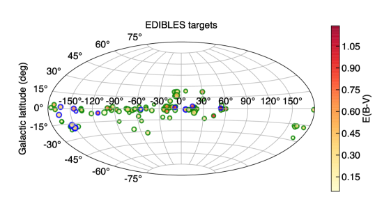
The target list is given in the Appendix, Table LABEL:tb:targetlist1 (their Galactic distribution is shown in Fig. 1). Columns (1) to (3) provide basic information on the target id (HD number) and coordinates (RA/Dec). Columns (4) and (5) list the spectral type and corresponding literature reference. The interstellar line-of-sight dust extinction properties, ${E}{\mathrm{(}B-V)}$, $R_{V}$, $A_{V}$, are given in columns (6) to (9). Columns (10) and (11) list the atomic and molecular hydrogen abundances with the molecular fraction $f_{\text{H}_{2}}$listed in column (12).

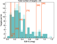
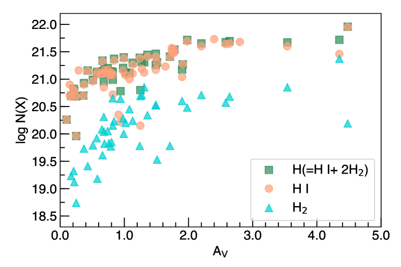
The total number of selected targets amounts to 114 (of which 96 have been observed at least once as of May 2017) and comprises mostly bright O and B stars ($V\approx$ 2–7 mag with a small fraction $7<V<9$ mag). The sample probes a wide range of interstellar dust extinction properties (${E}{\mathrm{(}B-V)}$$\sim$ 0–2 mag; $R_{V}\sim$ 2–6; $A_{V}\sim$ 0.1–4.5 mag) and molecular content ($f_{\text{H}_{2}}$$\sim$ 0.0–0.8). The histograms in Fig. 2 illustrate the range of parameters included in the survey sample. In Fig. 3 we show comparisons between visual extinction, $A_{V}$, and the measured neutral hydrogen column density $N$(H i), molecular hydrogen column density $N$(H₂), and total hydrogen column density $N$(H_tot) (=$N$(H i)+2$N$(H₂)). As noted above H₂ can be estimated using the CH transitions (Danks et al. 1984; Weselak et al. 2004).

5 Data processing

Acquiring high-S/N spectra with UVES is challenging in the context of EDIBLES for a number of reasons. For example, small errors in the wavelength calibration at the edges of individual adjacent orders can cause the appearance of ripples in the continuum in high-S/N exposures. Moreover, the unpredictable seeing and other observing conditions inherent in a filler programme mean that individual exposure times cannot be optimised for the actual sky conditions.

The overall quality of all 8 500 science and $\sim$ 1600 flat exposures was checked visually. This visual inspection led us to discard about 150 exposures that appeared corrupted. This could, for example, be due to sudden changes in weather conditions or premature termination of exposures. In addition, we carefully inspected for the presence of incorrect thorium-argon lamp, format-check, and flat field exposures that could result in faulty order tracing or wavelength calibration solutions (see also below).

Within a sequence of observations (20–40 minutes including overheads) the change in barycentric velocity correction is small ($<0.1$ km s^-1 per hour) so the spectra can be averaged without compromising the velocity precision. However, exposures taken on different nights were not averaged. This is to preserve multi-epoch information – specifically for spectroscopic binaries and the search for time-variable interstellar absorption – and to avoid addition of misaligned interstellar features due to variations in the barycentric velocity of the frame of the observer.

The data reduction was performed by two semi-independent teams, one using version 5.7.0 of the UVES pipeline (Ballester et al. 2000), esorex (version 3.12; ESO CPL Development Team 2015) integrated in a python pipeline (hereafter Reduction ’A’), and the other using the 4.4.8 version of the UVES pipeline (Reduction ’B’).

Each set of around 20 science frames was processed with the same set of calibration frames. For the format check, order definition and wavelength calibrations these were the nearest in time, with the master bias and master flats using frames taken typically over several days or weeks. In general, both data reductions used similar parameters for the different pipeline recipes, but with a few differences. Reduction ‘A’ adopts optimal merging, applies the blaze correction and uses about 100–130 flats for each arm, while reduction ‘B’ uses optimal merging and takes the nearest 140 flat field frames.

In the following we provide a detailed description of the different data processing steps and discuss their impact on the quality of the reduced spectra. The differences between reductions ‘A’ and ‘B’ are discussed in relation to the blaze correction and order merging step.

Figure 4: Comparison of the S/N of HD 23180 with changing number of flat frames. The S/N ratios plotted for each instrument setting are average values of S/N measured in five different continuum regions in the respective setting.

Bias

To subtract the CCD bias level in science frames, we created a master bias frame by median-stacking a set of 50 (reduction ‘A’) or 25 (reduction ‘B’) bias exposures, using the uves_cal_mbias recipe. To handle the bad columns in the REDL CCD, by default the recipe interpolates across bad pixels but does not apply this interpolation in science frames. This inconsistency creates boxy emission-like artifacts in the reduced spectra. To avoid this from occurring, high-quality bias frames are carefully pre-selected and the data are processed without interpolating over bad pixels.

Figure 5: (a) Part of the extracted spectrum of HD 23180 taken using the Red Lower EEV CCD (Red-L). (b) Ditto but for Red Upper MIT CCD (Red-U). The latter is a thick chip so fringing is much reduced compared with the EEV detector. The vertical scale is the same in both cases.

Order definition

In order to find the physical position of echelle orders in the X and Y directions of spectral frames for a given instrument setting, esorex uses a physical model based on the instrument configuration, ambient pressure, the humidity, slit width, central wavelength, camera temperature and CCD rotation angle. The physical model then predicts the X and Y pixel position corresponding to the nominal orders and stores the calculations into the guess line and order tables. These tables are then normally used as the initial values for identifying the specific positions of the orders.

To accurately detect the order positions, esorex defines a search box on the detected lines in the arc lamp frames and tries to match the predicted position of the physical model lines. The following procedure robustly detects the order positions:

1. measure the raw X and Y pixel positions of the thorium-argon lines on an arc frame exposure by defining a $\mathbf{60\times 60}$ pix² square search box,

2. compute the difference of predicted and detected order positions,

3. decrease the size of the search box to $\mathbf{40\times 40}$ pix², iterate the X and Y shifts to search for residuals less than $\mathbf{\pm 1}$ pixel and to reduce the root-mean-square (RMS) values,

4. fit a 2D Gaussian function to XY pixel positions within a ‘fit box’ centred at the predicted line positions,

5. For reduction ‘B’ additional iterations of the format check are done using different values of the CCD rotation offset, selecting the one with the maximum number of lines found,

6. and, finally, perform a 2D second-order polynomial fit in XY to the fitted line positions.

The highlighted values in the above steps are our tuned parameters in the uves_cal_predict recipe.

Figure 6: Close-up view of a region including two overlapping orders in the 564-nm setting for HD 23180 for both reduction ‘A’ (bottom red trace) and reduction ‘B’ (top black trace). The small jump in the continuum at approximately 5855 Å seen in reduction B (top black trace) is due to imperfect merging of two echelle orders. The apparent difference in S/N is due to alternative choices of wavelength sampling.

Table 2: Wavelength calibration uncertainties for the thorium-argon frames corresponding each of the observed UVES settings for HD 23180.

Arm	uncertainty (Å)	uncertainty (m s-1)
346-nm	$6.4\times 10^{-4}$	52
437-nm	$7.8\times 10^{-4}$	54
564-nm L	$4.5\times 10^{-4}$	26
564-nm U	$7.0\times 10^{-4}$	34
860-nm L	$8.3\times 10^{-4}$	33
860-nm U	$1.1\times 10^{-3}$	36

Flat fielding

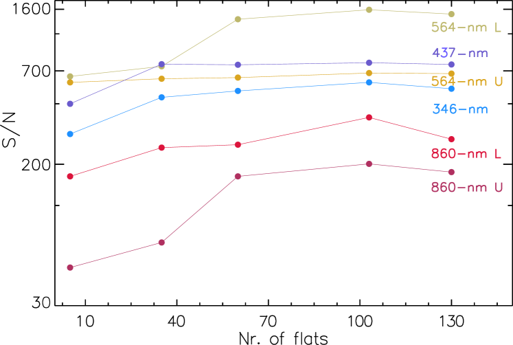
The flat-fielding is applied, to the 2D frame, before the order extraction (see below). This is known as the pixel flat-fielding method. The standard UVES pipeline uses only five flat field frames, which limits the maximum S/N. To demonstrate the necessity for accurate flat-fielding to reach the required S/N ratio, we reduced 11 science frames of HD 23180 using a different number of flat field frames to build the master flat frame. As shown in Fig. 4, increasing the number of flat fields helps to increase the final S/N. More than 100 flat field frames do not cause the S/N to increase further, indicating that flat fielding is no longer the limiting factor on the S/N. In the case of the 860-nm setting the S/N drops between 100 and 130 applied flats due to the presence of several bad-quality flat frame exposures. For the final reduction these were rejected and we selected as many as possible, usually about 100, good quality flat frames. By using the additional flat fields, we were able to improve the final S/N by factors of two to five, depending on the wavelength.

Note that the intensity (photon counts) of normal flats are very low in the UV ($<$320 nm). Therefore, to improve the quality of the first-orders of the 346-nm arm spectra, a final master flat is constructed by combining a set of normal flats with flats obtained by exposing with a deuterium calibration lamp. The merging was done at orders 145 and 146 around 321 nm with the master deuterium-lamp flat being used bluewards of this and the normal flat redwards. This is to avoid as much as possible spurious absorption-line features in the final science spectrum caused by emission features in the deuterium lamp redwards of 321 nm.

Table 3: Median S/N per “resolution-element” (0.04 Å spectral bin) for each UVES setting/arm configuration for all available EDIBLES spectra.

Setting	Arm	$\lambda$-range (nm)	Median S/N	Sample
			(0.04 Å bin)	size
346	blue	339.3 – 339.4	780	204
437	blue	398.8 – 398.9	1070	187
564	red-L	511.0 – 511.1	1090	205
	red-U	613.1 – 613.2	1020	205
860	red-L	675.35 – 6754.55	670	184
	red-U	869.9 – 870.0	880	183

Figure 7: Comparison between the ADP and EDIBLES processing of HD184915 spectra (0.02 Å binsize). The S/N measurements, taken at 4912–4913 Å and 6129–6130 Å for the Red-L and Red-U spectra, are given in the top and bottom panel. Resampling to 0.04 Å binsize (i.e. corresponding to the spectral resolution) further increases the S/N by factor $\sqrt{2}$.

Figure 8: EDIBLES UVES spectra of HD 170740 (B2 V) for each setting from top to bottom: 346B, 437B, 564L, 564U, 860L, 860U. This overview figure is a demonstration of the data quality. The main gaps in wavelength coverage are between 5610–5670 Å and 8530–8680 Å which correspond to the physical separation of the Red-L and Red-U detectors in both the 564 and 860-nm settings. Note also the inter-order gaps, several are indicated with arrows, in the 860-nm Red-U spectrum above $\sim$9600 Å as well as several conspicuous regions containing bands of closely-spaced telluric absorption lines (indicated with red horizontal bars) mostly in the Red-L and Red-U 860-nm spectra (bottom two panels). Two order-merging jumps are indicated in the fourth panel. A more detailed version of this figure is shown in the appendix (Fig. 15) where specific interstellar species are labeled and a synthetic DIB spectrum is shown for comparison.

Order extraction

Various possible extraction methods were tested and we find that the average extraction method with performing a flat fielding before the extraction (see above) leads to a higher S/N with respect to other methods (such as optimal extraction), which is generally the case for high S/N spectroscopy. This method also reduces the fringing seen in the red wavelengths $\geq$ 700 nm, although does not entirely remove it. Fig. 5 shows that displays parts of an extracted science spectrum near the gap between the upper and lower CCDs. The fringing is much worse in the lower thinned EEV chip than in the upper MIT thick chip (Smoker et al. 2009).

Cosmic ray rejection and hot pixels

To remove the cosmic rays and possible hot pixels we applied a sigma-clipping method to each extracted spectrum. The default sigma-clipping threshold value in esorex is $\kappa=10$, but to identify all induced hot pixels we set this $\kappa=6$ to be sure that all cosmic/hot pixels are removed and no real data are clipped.

Wavelength calibration

UVES wavelength calibration errors are typically in the range of 0.1–0.5 km s^-1 (Whitmore et al. 2010). To achieve an accurate wavelength calibration, the dispersion relation is obtained by extracting the thorium-argon arc lamp frames using the same weights as those used for the science objects. Therefore, first we reduced the science frames with an optimal extraction method to generate a pixel weight map. Then by applying this weight map to the wavelength calibration, an accurate wavelength calibration with a statistical error less than $5\times 10^{-4}$ Å typically in all central wavelengths (for more details see Table 2) and a systematic uncertainty less than $1.7\times 10^{-4}$ Å is achieved. To optimize the number of lines used in the wavelength calibration solution we tested a tolerance value $\simeq 0.07$ pixels to reject the line identification with wavelength residuals worse than the tolerance. For the final iterations of the fit of the wavelength calibration solutions we set the sigma-clipping to $\kappa=3$. Further improvements to the wavelength calibration are being studied for the public release of the data. For example, there is a temperature and density dependent shift (which can be as much as 1 pixel and different for the different wavelength regions) in the position of the thorium-argon lines (UVES User Manual). This can be potentially corrected by taking into account the difference between the observation and calibration temperatures and pressures. Also, we foresee improvements to the final wavelength calibration in the 860 nm Red-U arm, where there are few thorium-argon lines, by cross-referencing with a model telluric transmission spectrum.

Figure 9: (Left) Example of telluric line correction in the weak line regime by means of the rope-length method applied to the spectrum of HD 170740. Telluric lines of O₂ are corrected first, then H₂O lines. (Right) Example of telluric line correction in the strong line regime by means of a two-step method and a composite instrumental profile adjustment (see text). Residuals remain at the location of the deepest lines, especially when the model does not predict their shape and exact Doppler shift very accurately. The positions of the 9577 and 9632 Å DIBs attributed to C${}_{60}^{+}$ are indicated.

Blaze function and order merging

Previous analyses of data obtained with UVES demonstrate that the shape and position of the blaze function is the primary source of problems in the order overlap regions. The continuum changes vary smoothly over subsequent orders, which may be related to the fact that the blaze profiles produced by UVES are not the same as the theoretical predictions. Accordingly, the blaze function at the overlapping regions is not sufficiently well characterised, therefore by averaging the overlap regions some artificial features appear and cause the signal level to fall off at the end of the orders. Irregular variations in the continua at the edges of orders are likely due to a mismatch between the paths of the light from the star and the flat-field lamp (Nissen 2008) and result in discontinuities where orders have been merged.

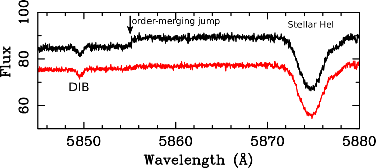
For reduction ‘B’, no blaze correction was performed. Optimal merging provided the best results in the overlapping regions for both reductions ‘A’ and ‘B’. Fig. 6 shows a comparison of reductions ‘A’ and ‘B’ for HD 23180 in a spectral region with two overlapping orders. Reduction ‘B’ reveals a mismatch of the order-overlapping regions, resulting in a jump in the spectra at 5855 Å not present in the reduction ‘A’ spectrum.

Quality control

The S/N of the spectra as a function of wavelength was estimated by fitting a first order polynomial to regions of the spectra in bins of 1 Å  and measuring the residual in each 0.02 Å wavelength bin. Table 3 lists the median S/N (per 2-pixel “resolution-element”) for each setting, together with the respective continuum wavelength regions. In Fig. 7 we compare for HD 184915 the spectra obtained with the dedicated EDIBLES processing presented here and the default archive data products (ADP) provided by ESO. The increase in S/N (labelled in the figure) is almost a factor two for both the Red-L and Red-U spectra (cf. Table 1). For each target the different settings/arms generally have different S/N ratios. This is primarily due to (1) the choice of targets which are often brighter in V band compared to B band (i.e. reddening), and (2) the lower efficiency of UVES in the very blue and very red parts of the accessible wavelength range. In terms of S/N reduction ‘A’ performs slightly better than reduction ’B’ for the 346-nm setting, both perform similar for the 437-nm and 860-nm settings, while reduction ‘B’ performs better for the 564-nm setting. The main difference between the two reductions is in terms of the order-merging jumps. In addition, there are small, though noticeable differences in the ‘noise’ between both reductions. The reduction scheme ‘A’ is adopted as the primary scheme for results shown in this work. Both reductions are therefore retained for reference and as a control for spurious features.

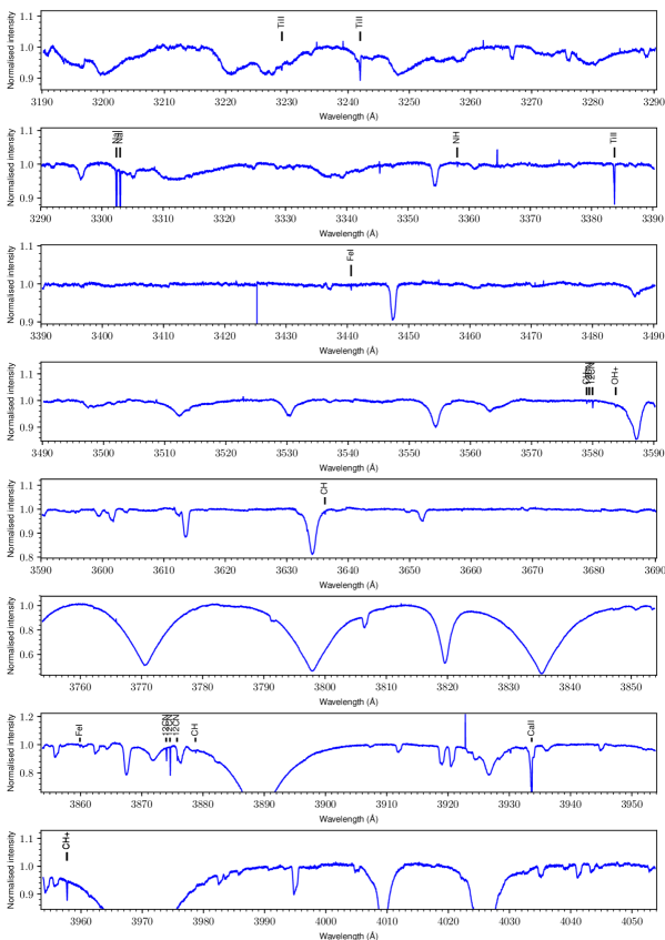
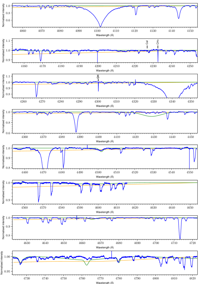
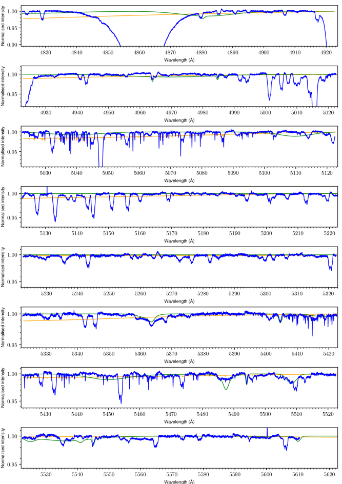
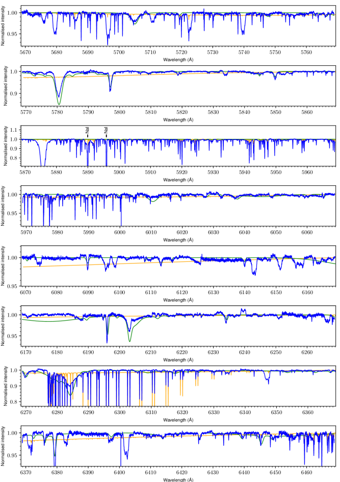
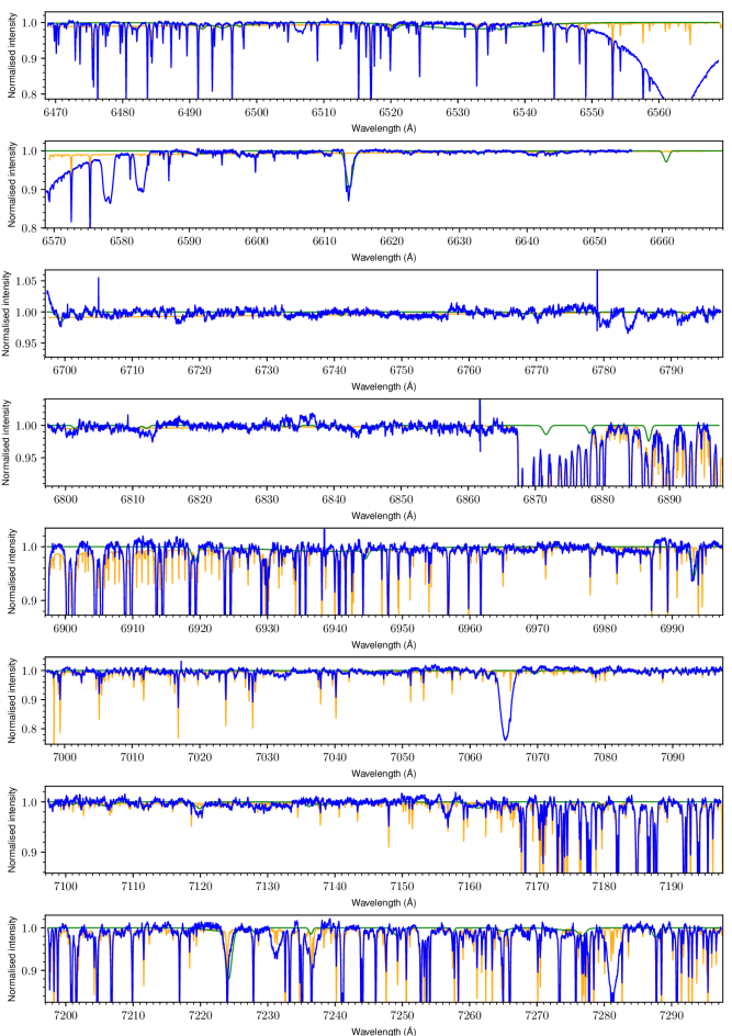
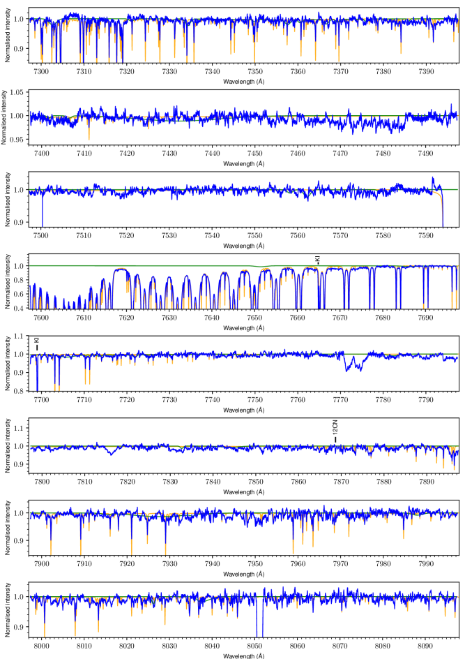
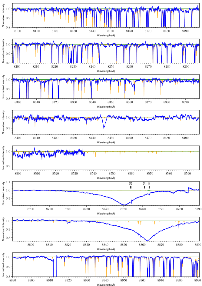
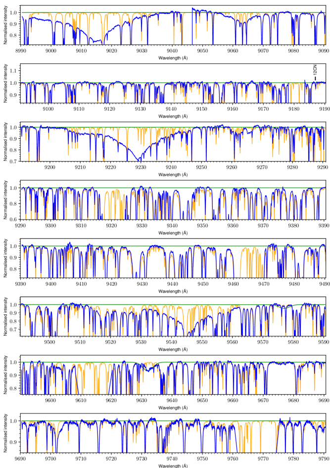
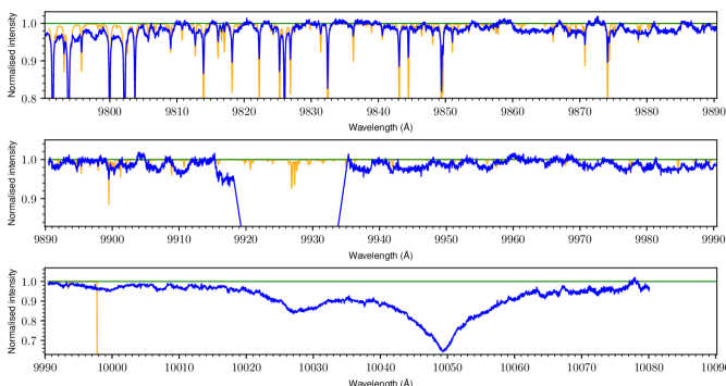
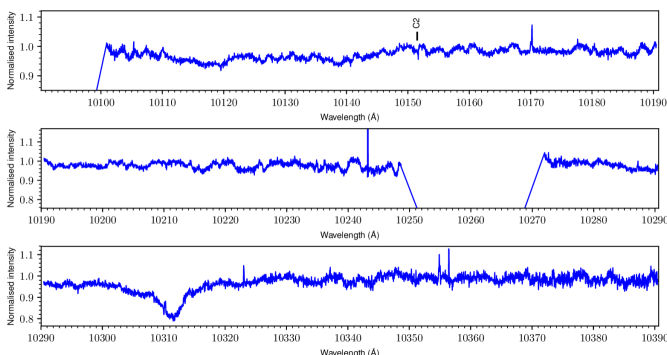
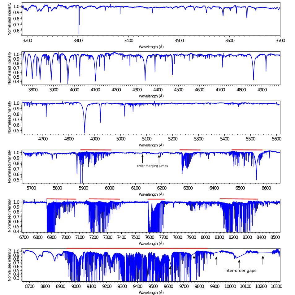
As an example, the final continuum normalised EDIBLES UVES spectrum of HD 170740 (from reduction ‘A’) is shown in full in Fig. 8, where each panel corresponds to one of the instrument settings (Table 1). A closer view of this spectrum in shown in Appendix B. All processed EDIBLES spectra will be released as new “Phase 3” data to the ESO archive later in the project.

6 Telluric and stellar features

6.1 Earth transmission spectrum

A large number of weak and strong telluric oxygen and water absorption bands arise from molecules present in the Earth atmosphere covering nearly the full DIB range. In addition, for the near-UV spectral domain (300–350 nm) a correction for atmospheric ozone needs to be applied.

These telluric lines can be removed or modelled by using bright, early-type type star spectra recorded in the same conditions as the targets, or by using synthetic atmospheric transmittance spectra. The former method requires observing (unreddened) standard stars at roughly similar airmass, shortly before or after the primary science target observations. This procedure is not possible within the filler observation strategy, and as the EDIBLES targets are themselves bright this would double the required observing time. The latter method has the advantage of saving observing time, avoiding features associated with the standard star and benefits from the increase in quality and availability of the molecular databases. The first tests of atmospheric spectra correction were performed based on the following approach:

First, the telluric transmittance is optimally adapted to each target. Paranal observing conditions are downloaded from the TAPAS facility (Bertaux et al. 2014). The TAPAS transmittance spectra are based on the latest HITRAN molecular database (Rothman et al. 2013), radiative transfer computations (Line-By-Line Radiative Transfer Model; Clough & Iacono 1995), and are computed for atmospheric temperature, pressure and composition interpolated by the ETHER data centre based on a combination meteorological field observations and other information.

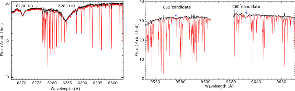
Then, in regions of moderate absorption (i.e. less than 70% at line centers before instrumental broadening), a simple method called rope-length minimization is used (Raimond et al. 2012). Briefly, the algorithm searches for the minimal length of the spectrum that is obtained after division of the data by the transmittance model. To do so the column of the absorbing species, the Doppler shift and the width of the instrumental function by which the transmittance model is convolved are all tuned. The method uses the fact that when the telluric lines are not well reproduced, strong maxima and minima remain after the data-model division and the spectrum length increases. On the contrary, if the modelled lines follow very well the observed ones, the corrected spectrum is smooth. An example of correction is shown in Fig. 9 for the 6284 Å DIB. Here the rope-length method has been first applied to the O₂ lines, then in a subsequent step the O₂-corrected spectrum is corrected for the weak H₂O lines that are also present in this spectral region.

For regions of stronger telluric lines, division by deep lines induces overshoot and the exact shape of the telluric profiles and of the instrumental function becomes crucial. The simple rope-length method alone is no longer appropriate. We have tested an iterative method that is a combination of the rope-length method and a classical fitting. In a first step we excluded all spectral intervals around the centres of the deep lines and performed a segmented rope-length optimization, i.e. the algorithm searches for the model parameters that minimize the sum of the lengths of the individual spectral segments. We then divided the data by the corresponding adjusted model and performed a running average of the divided spectrum to obtain an approximate stellar continuum. We then fitted the data to the convolved product of this continuum and a telluric transmittance. The instrumental function is now modelled as the sum of a Gaussian and a Lorentzian, which allows weak extended wings to be taken into account. The instrumental profile is the same for all lines within the corrected interval. The parameters defining these two components as well as the column of the absorbing species are free to vary during the adjustment. The data were then divided by this updated model. This process can be iterated and stopped when there is no longer any decrease of the ”rope-length”. An example of such a two-step correction is shown in Fig. 9 for the spectral region of the C${}_{60}^{+}$ 9577 and 9632 Å DIBs. There are still some residuals, but these are limited mostly to the deepest, (partially) saturated telluric lines. This occurs particularly when these lines are slightly Doppler shifted or broadened due to atmospheric pressure in a way that is not fully predicted by the model. For a description of such effects see Bertaux et al. (2014). Nevertheless, the DIBs at 9577 and 9632 Å, assigned to be due to C${}_{60}^{+}$ as mentioned in the introduction, stand out clearly in the telluric corrected spectrum. The three weaker DIBs between 9350 and 9450 Å reported by Walker et al. (2015), though not yet confirmed independently (Galazutdinov et al. 2017; Cordiner et al. 2017) present significant challenges for detection due to the presence of strong, saturated telluric water lines in this spectral range. We intend to investigate the C${}_{60}^{+}$ bands in more detail later in the EDIBLES project, but this will depend upon the accuracy and success of the telluric line modelling for each line-of-sight (as there are numerous saturated atmospheric water absorption lines in this wavelength region) as well as the stellar atmosphere modelling required to account for, for example, contribution of Mg ii (as discussed in Galazutdinov et al. 2017).

Figure 10: An illustration of the quality of the spectra for the 5780 and 5797 Å (left) and 6614 Å (right) DIBs. For each target all observed spectra were co-added in the heliocentric reference frame. The five targets shown have comparable E(B-V) values (Tables LABEL:tb:targetlist1 and LABEL:tb:targetlist2), and thus have similar 5797 Å DIB strengths. The well established, strongly variable 5780/5797 ratio can be seen in the spectra, with the intensity of 5780 absorption inversely related to the molecular gas fraction, $f_{\text{H}_{2}}$ (Tables LABEL:tb:targetlist1 and LABEL:tb:targetlist2). The five spectra are shown superimposed on each other at the top of the panels. Note that because of generally poor observing conditions there are numerous weak and narrow atmospheric water features present (particularly noticeable around 5788–5792 Å) that could influence the 5797 Å profile. In the future these features will be removed using the method described in Sect. 6.

6.2 Stellar spectra

In addition to the goals discussed above, the EDIBLES observations provide high-quality spectra of the target stars themselves. These span the full spectral range of early-type stars, from early O-type dwarfs through to late B-type supergiants (plus a couple of later/cooler stars). Published spectral classifications of the sample are summarised in Tables LABEL:tb:targetlist1 and LABEL:tb:targetlist2.

All of the O-type EDIBLES targets have been observed as part of the Galactic O-Star Spectroscopic Survey (GOSSS), a comprehensive survey of bright Galactic O stars at a resolving power of $R$ $\sim$2500 (Sota et al., 2011, 2014). The detailed O-star classifications quoted in Tables LABEL:tb:targetlist1 and LABEL:tb:targetlist2 are the GOSSS types – a thorough description of the classification criteria was given by Sota et al. (2011), including an overview of the various classification qualifiers used to convey additional information on the spectra (their Table 3).

In contrast, most of the B-type stars in the EDIBLES sample have not been subject to such morphological rigour with high-quality digital spectroscopy. Work is underway within the GOSSS to better define spectral standards and the classification framework for early B-type stars (Villaseñor et al. in prep.), with a few stars overlapping with the EDIBLES sample. Nonetheless, the high-quality, high-resolution spectra from EDIBLES will be useful to refine the classification framework for B-type stars, particularly compared to similar efforts in the Magellanic Clouds (e.g. Evans et al., 2015).

In the short-term we will inspect the EDIBLES data in the context of classification, to update/refine spectral types as required – whether arising from the added information of the high-resolution UVES data (cf. lower-resolution spectroscopy from the GOSSS, for example), or simply from intrinsic spectral variability, which is seen in many early-type stars. This will ensure the best parameters are adopted in estimating stellar colours, thence the line-of-sight extinctions. We will also look for evidence of spectroscopic binaries in targets with multiple observations (and/or relevant archival data, see, e.g., Sect. 7.4). Our longer-term objective is a quantitative analysis of the stellar spectra to determine their physical parameters (effective temperature, gravities, rotational velocities, mass-loss rates etc), employing tools developed specifically for the analysis of early-type spectra (e.g. Mokiem et al., 2005; Simón-Díaz et al., 2011). Ultimately this will help removal of stellar features from the EDIBLES spectra to aid analysis of the interstellar features.

7 Quality assessment: the interstellar spectrum

In this Section we highlight the interstellar lines and bands observed for a few selected lines-of-sight.

7.1 EDIBLES

As noted above, the full spectrum of HD 170740 is shown as an example in Figs. 8 and 15. For initial guidance in identifying the DIBs in this line-of-sight the average ISM DIB spectrum (Jenniskens & Désert 1994), scaled to ${E}{\mathrm{(}B-V)}$= 0.5 mag, is shown in the latter figure. This reference spectrum includes broad DIBs not included in e.g. Hobbs et al. (2009) but which appear to be present in the observed spectrum.

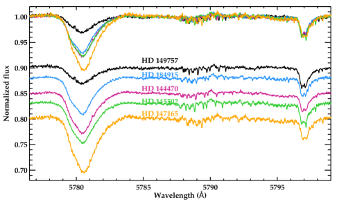
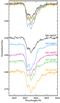
In Fig. 10 we compare the three strong DIBs at 5780, 5797 Å (Heger 1922; Merrill & Wilson 1938) and 6614 Å for single-cloud lines-of-sight towards five EDIBLES targets, HD 149757, HD 184915, HD 144470, HD 145502, and HD 147165. The line of sight reddening, ${E}{\mathrm{(}B-V)}$, for these sightlines differs by less than 0.17 mag (c.f. Table LABEL:tb:targetlist1). The spectra are averages of individual exposures co-added in the heliocentric rest frame and subsequently continuum normalised (but not otherwise scaled other than to offset them in the figure).

As expected, for sightlines with such small variations in reddening, the 5797 Å DIB profiles have similar central depths (insensitive to $f_{\text{H}_{2}}$; Cami et al. 1997). The large variations in the strength of the 5780 Å DIB are thought to be related to variations in the local interstellar conditions. The sightline with the weakest 5780 Å DIB is more neutral as indicated by the large molecular fraction, whereas the sightline with the strongest 5780 Å DIB has the highest atomic column density. However, while the 6614 Å DIB of the former is also the weakest, the latter does not exhibit the strongest 6614 Å DIB, thus indicating that additional parameters must play a role in determining the DIB carrier column density.

7.2 EDIBLES versus CES

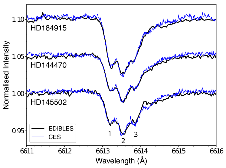
High-resolution (R = 220,000) spectra of the 6614 Å band have been recorded using the Coude Échelle Spectrograph (CES) fed by the fibre link with the Cassegrain focus of the 3.6 m telescope at La Silla Observatory (Galazutdinov et al. 2002). A signal-to-noise of $\sim$600–1000 was achieved. Comparison of the EDIBLES and CES data is shown in Fig. 11 for HD 184915, HD 144470 and HD 145502 and the main features are in good agreement. Of the three principal absorption components, the shortest wavelength feature (component 1) is relatively strong for HD 184915 in both studies, whereas components 1 and 3 have comparable intensities for the lines-of-sight towards HD 144470 and HD 145502. No significant additional structure is evident in the higher resolution CES spectra.

Figure 11: Comparison of the 6614 Å DIB for HD 184915, HD 144470, and HD 145502 obtained with EDIBLES (black solid line; this work, $R\sim 110\,000$) and the CES (blue solid line; Galazutdinov et al. 2002; $R\sim 220\,000$). The sub-structure components 1, 2, and 3 are labelled in the bottom trace (see text).

Figure 12: Comparison of the 6614 Å DIB for HD 147888 ($\rho$ Oph D) obtained with EDIBLES (this work, $R\sim 110\,000$) and the AAT (Cordiner et al. 2013, $R\sim 58\,000$). The top spectrum labeled “ADP” is the spectrum obtained with the standard ESO archive pipeline processing (i.e. using the default number of 5 flat-field frames). The red dotted line represents the telluric absorption spectrum, shifted to match the heliocentric rest frame of each target; highlighting the presence of a small telluric absorption feature at 6614/6614.5 Å.

Figure 13: Comparison of EDIBLES (black) and UVES POP (red) spectra of HD 169454 for interstellar lines of NH($\lambda\lambda$3353.92, 3358.05 Å) (top) and CN(1-0) ($\lambda\lambda$3579.45, 3579.96, and 3580.9 Å; Meyer et al. 1989) (bottom); the telluric spectrum is shown in orange. HD 169454 is a blue supergiant (B1 Ia) – the broad stellar line in the spectrum is He i $\lambda$3355 Å.

Figure 14: Comparison of EDIBLES (black) and UVES POP (red) spectra of HD 148937 (O6 f?p) for the interstellar Na lines (UV, top left; D, top right) and DIBs at $\lambda\lambda$5480–5545 Å (lower left) and $\lambda\lambda$6360–6379 Å (lower right). The telluric spectrum is shown in orange, and the average ISM DIB spectrum in green. The apparent feature at 6384 Å in the UVES POP data (bottom right panel) is related to the order merging, but the significant change in the He i 5876 line (top right panel) appears astrophysical in nature.

7.3 EDIBLES versus AAT

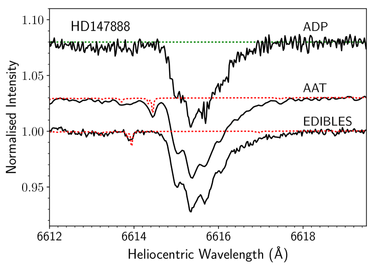
To assess the quality of our spectra with respect to previous studies, we compared our EDIBLES spectrum of HD147888 (obtained in a single exposure on 2016-08-08) with a spectrum obtained using the Anglo-Australian Telescope (AAT) in June 2004 by Cordiner et al. (2013). The AAT spectra were obtained using the UCLES instrument at a resolving power of 58 000 and have S/N $\sim$ 900. Cordiner et al. (2013) reduced their data using a custom procedure, taking special care to optimally correct for CCD non-linearity, scattered light subtraction and flat fielding, as well as wavelength calibration. A comparison between the EDIBLES and AAT spectra is shown in Fig. 12 for the 6614 Å DIB, which makes for a good general test case due to the presence of narrow and broad features within its profile. Apart from differences in the wavelengths of the telluric features, and a slight difference in the overall spectral slope (presumably due to uncorrected differences between the UVES and UCLES blaze functions), the spectra are almost identical within the noise. Slight differences in the depths and widths of the substructure peaks are attributable to the higher resolution of the UVES spectrum. The overall excellent match demonstrates the quality of our EDIBLES reduction procedure. For reference we show also the ADP spectrum, which uses only 5 flat-field frames; the large increase in S/N when using our custom flat-field processing is apparent.

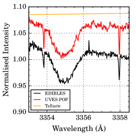
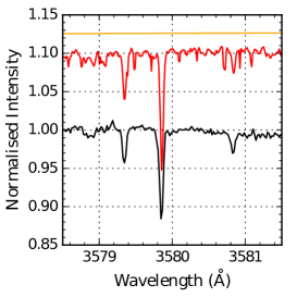
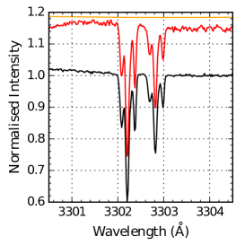
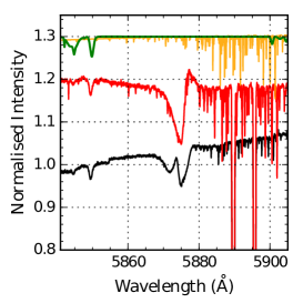
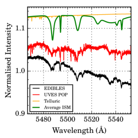
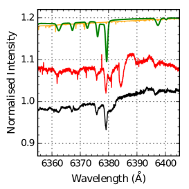
7.4 EDIBLES versus UVES POP

To further illustrate the quality of the data we compared spectra of two targets, HD 148937 (Fig. 14) and HD 169454 (Fig. 14), which were both observed as part of the EDIBLES survey and the UVES Paranal Observatory Project (POP; Bagnulo et al. 2003). The UVES POP programme gathered a library of high-resolution, high S/N spectra of (field) stars across the Hertzsprung-Russell diagram. The spectra in the figures have been scaled in intensity to facilitate comparison, but not continuum normalised.

Fig. 14 shows the NH and OH⁺ lines in the sightline towards HD 169454. The top panels in Fig. 14 compare the sodium doublets at $\sim$3303 Å (see also Hunter et al. 2006) and $\sim$5895 Å for the sightline towards HD 148937. The bottom panel compares several weak and strong DIBs in the HD 148937 line-of-sight. In each panel the EDIBLES and UVES POP spectra are shown in black and red, respectively. The average ISM synthetic DIB spectrum (adapted from Jenniskens & Désert 1994) is shown in green and a generic Paranal model telluric spectrum is shown in orange. The agreement between stellar and interstellar features in the EDIBLES and UVES POP is excellent, where the EDIBLES data generally reach a higher S/N.

The two right-hand panels of Fig. 14 reveal apparent variations between the EDIBLES data compared to the UVES POP spectrum. The strong absorption in the POP data at $\sim$6384 Å coincides with the order ends/overlap, and appears to be an artefact of the order merging. In contrast, the significant change in the He I 5876 absorption seems robust. In the context of HD 148937 being a peculiar magnetic star, this variation is quite remarkable. This aspect will be discussed elsewhere.

These comparisons with existing data for selected sightlines show the excellent data quality of the spectra acquired within EDIBLES, illustrating its potential for detailed studies of physical conditions and DIB properties in the diffuse ISM.

8 Summary

In this first of a series of papers we have presented the design and scope of the ESO Diffuse Interstellar Bands Large Exploration Survey (EDIBLES). We presented the scientific goals and the immediate objectives of EDIBLES, along with the survey sample and its characteristics.

At the time of writing (May 2017), spectra had been acquired for 96 targets from 114 in the overall programme. These spectra cover the wavelength range from 305 to 1042 nm at a spectral resolving power of $\sim$70 000–110 000. We have presented the data-processing steps employed to reduce the survey data so far.

The median S/N ratio (per 0.04 Å spectral bin) varies from $\sim$600–700 hundred in the blue ($<$400 nm) and near-infrared ($>$800 nm) ranges, to $\geq$1000 in the green-red (500–700 nm). To illustrate the quality and scope of the new spectra we have compared (1) EDIBLES and AAT spectra of the 6613 Å DIB towards HD 147888, (2) EDIBLES and CES spectra of the 6613 Å DIB for the sightlines towards HD 184915, HD 144470 and HD 145502, and (3) EDIBLES and UVES POP spectra of HD 148937 and HD 169454.

Upcoming papers in this series will present in detail the array of scientific results that are being explored with the EDIBLES data set. Once the program is completed the advanced data products (merged and normalised spectra) will be released to the community through the ESO Science Archive and the CDS/ViZieR service.

Appendix A Survey sample

Table LABEL:tb:targetlist1 lists spectral classifications and line-of-sight parameters for the observed EDIBLES targets to date; Table LABEL:tb:targetlist2 lists the additional observations that will supplement the data discussed here in due course. The $R_{V}$ and $A_{V}$ extinction values are taken (in order of preference) from Valencic et al. (2004), Fitzpatrick & Massa (2007), or Wegner (2003). H i and H₂ column densities are from Jenkins (2009). The interstellar reddening, ${E}{\mathrm{(}B-V)}$, was computed from $(B-V)_{J}$ colours (taking the average from Tycho-2 and Simbad $B-V$ colours; where Tycho-2 colours were converted to Johnson colours; Mamajek et al. 2002) and the published spectral classifications, adopting intrinsic colours from Fitzgerald (1970).

References for the spectral classifications in col. 4 of both tables are: M50 (Morgan & Roman 1950); S52 (Sharpless 1952); M55 (Morgan et al. 1955); H56 (Hiltner 1956); S56 (Stebbins & Kron 1956, classification originally from W. W. Morgan); F57 (Feast et al. 1957); O59 (Osawa 1959); G68 (Guetter 1968); L68 (Lesh 1968); A69 (Abt & Morgan 1969); C69 (Cowley et al. 1969); H69 (Hiltner et al. 1969); S71 (Schild & Chaffee 1971); W71 (Walborn 1971); H73 (Humphreys 1973); M73 (Morgan & Keenan 1973); L75 (Levato 1975); L76 (Levato & Abt 1976); W76 (Walborn 1976); G77 (Garrison et al. 1977); H78 (Houk 1978); H82 (Hendry 1982); G94 (Garrison & Gray 1994); M95 (Massey et al. 1995); P98 (Parsons & Ake 1998); S99 (Steele et al. 1999); G01 (Gray et al. 2001); E05 (Evans et al. 2005); L06 (Levenhagen & Leister 2006); R09 (Renson & Manfroid 2009); S11 (Sota et al. 2011); H13 (Holberg et al. 2013); S14 (Sota et al. 2014).

Table 4: Targets observed for EDIBLES.

Identifier	RA	Dec	Spectral type	Ref.	${E}{\mathrm{(}B-V)}$	$R_{V}$	$A_{V}$	Ref	log $N$(H i)	log $N$(H2)	$f_{H_{2}}$
	J2000	J2000			mag		mag		cm-2	cm-2
HD 22951	03:42:22.7	$+$33:57:54.1	B0.5 V	M55	0.23	–	–		21.04	20.46	0.35
HD 23016	03:42:19.0	$+$19:42:00.9	B8 Ve	S99	0.05	2.30	0.12	W03	–	–	–
HD 23180	03:44:19.1	$+$32:17:17.7	B1 III	G77	0.28	3.11	0.93	V04	20.88	20.60	0.51
HD 24398	03:54:07.9	$+$31:53:01.1	B1 Ib	L68	0.29	2.63	0.89	W03	20.8	20.67	0.60
HD 27778	04:23:59.8	$+$24:18:03.6	B3 V	O59	0.36	2.59	0.91	V04	20.35	20.72	0.82
HD 34748	05:19:35.3	$-$01:24:42.8	B1.5 Vn	L68	0.13	2.61	0.29	W03	21.16	–
HD 36486	05:32:00.4	$-$00:17:56.7	O9.5 II Nwk	S11	0.16	–	–		20.19	14.68	0.00
HD 36695	05:33:31.5	$-$01:09:21.9	B1 V	L68	0.08	2.45	0.15	W03	20.7	–	–
HD 36822	05:34:49.2	$+$09:29:22.5	B0 III	L75	0.14	2.64	0.21	W03	20.81	19.32	0.06
HD 36861	05:35:08.3	$+$09:56:03.0	O8 III ((f))	S11	0.13	2.46	0.22	W03	20.78	19.12	0.04
HD 37022	05:35:16.5	$-$05:23:23.2	O7 Vp	S11	0.31	5.73	1.78	V04	21.54	17.55	0.00
HD 37041	05:35:22.9	$-$05:24:57.8	O9.5 IVp	S11	0.21	5.67	1.13	V04	–	–	–
HD 37061	05:35:31.4	$-$05:16:02.6	B0.5 V	S71	0.52	4.29	2.40	V04	–	–	–
HD 37367	05:39:18.3	$+$29:12:54.8	B2 IV-V	L68	0.37	3.55	1.49	V04	21.17	20.53	0.31
HD 37903	05:41:38.4	$-$02:15:32.5	B1.5 V	S52	0.34	3.74	1.31	V04	21.12	20.85	0.60
HD 38771	05:47:45.4	$-$09:40:10.6	B0.5 Ia	W71	0.07	–	–		20.52	15.68	0.00
HD 40111	05:57:59.7	$+$25:57:14.1	B1 Ib	L68	0.11	3.05	0.37	W03	20.9	19.73	0.12
HD 41117	06:03:55.2	$+$20:08:18.4	B2 Ia	W71	0.41	3.12	1.25	V04	20.15	20.69	0.87
HD 43384	06:16:58.7	$+$23:44:27.3	B3 Iab	L68	0.54	3.29	1.91	W03	21.27	–	–
HD 53975	07:06:36.0	$-$12:23:38.0	O7.5 Vz	S11	0.20	3.25	0.62	W03	21.13	19.18	0.02
HD 54439	07:08:23.2	$-$11:51:08.6	B2 IIIn	M55	0.27	2.73	0.79	V04	–	–	–
HD 54662	07:09:20.3	$-$10:20:47.8	O7 Vz var? (SB2)	S14	0.32	3.12	0.81	W03	21.38	20.00	0.08
HD 55879	07:14:28.3	$-$10:18:58.5	O9.7 III	S11	0.13	2.47	0.15	W03	20.9	–	–
HD 57061	07:18:42.5	$-$24:57:15.8	O9 II (SB2+SBE)	S14	0.12	3.57	0.36	W03	20.7	15.48	0.00
HD 66194	07:58:50.6	$-$60:49:28.1	B2 Vne	A69	0.15	2.25	0.41	W03	–	–	–
HD 66811	08:03:35.1	$-$40:00:11.3	O4 I(n)fp	S14	0.08	5.01	0.25	W03	19.96	14.45	0.01
HD 73882	08:39:09.5	$-$40:25:09.3	O8.5 IV (SB1+SBE)	S14	0.68	3.56	2.46	V04	21.11	21.08	0.65
HD 75309	08:47:28.0	$-$46:27:04.0	B2 Ib/II	H78	0.16	3.53	1.02	V04	21.07	20.20	0.21
HD 75860	08:50:53.2	$-$43:45:05.4	BC2 Iab	W76	0.87	3.44	3.10	W03	–	–	–
HD 79186	09:11:04.4	$-$44:52:04.4	B5 Ia	H69	0.28	3.21	1.28	V04	21.18	20.72	0.41
HD 80558	09:18:42.4	$-$51:33:38.3	B6 Ia	H69	0.57	3.35	2.01	W03	–	–	–
HD 81188	09:22:06.8	$-$55:00:38.4	B2 IV	L75	0.10	–	–		19.95	17.70	0.01
HD 91824	10:34:46.6	$-$58:09:22.0	O7 V((f))z (SB1)	S14	0.25	3.35	0.80	V04	21.12	19.85	0.10
HD 93030	10:42:57.4	$-$64:23:40.0	B0.2 Vp	W76	0.08	2.43	0.10	W03	20.26	15.02	0.00
HD 93205	10:44:33.7	$-$59:44:15.5	O3.5 V((f)) + O8 V	S14	0.34	3.25	1.24	V04	21.38	19.78	0.05
HD 93222	10:44:36.2	$-$60:05:29.0	O7 V((f))z	S14	0.34	4.76	1.71	V04	21.4	19.78	0.05
HD 93843	10:48:37.8	$-$60:13:25.5	O5 III(fc) SB1?	S14	0.27	3.89	0.66	V04	21.33	19.61	0.04
HD 94493	10:53:15.1	$-$60:48:53.2	B0.5 Ib:	H73	0.23	3.57	0.82	V04	21.08	20.15	0.19
HD 99953	11:29:15.1	$-$63:33:14.2	B2 Ia	M55	0.45	3.69	1.77	V04	–	–	–
HD 103779	11:56:58.0	$-$63:14:56.7	B0.5 Iab	G77	0.24	3.29	0.69	V04	21.16	19.82	0.08
HD 104705	12:03:23.9	$-$62:41:45.8	B0.5 III	M55	0.23	2.81	0.65	V04	21.1	20.08	0.16
HD 109399	12:35:16.5	$-$72:43:00.8	B0.5 Ib	H73	0.26	3.26	0.68	W03	21.11	20.04	0.15
HD 111934	12:53:37.6	$-$60:21:25.4	B1.5 Ib	E05	0.34	2.45	1.25	V04	–	–	–
HD 112272	12:56:33.7	$-$64:21:39.2	B0.5 Ia	M55	0.85	3.09	3.09	V04	–	–	–
HD 113904	13:08:07.2	$-$65:18:21.7	O9 III	S14	0.20	3.63	0.76	W03	21.08	19.83	0.10
HD 116852	13:30:23.5	$-$78:51:20.5	O8.5 II-III((f))	S14	0.20	2.42	0.51	V04	20.96	19.79	0.12
HD 122879	14:06:25.2	$-$59:42:57.3	B0 Ia	W76	0.34	3.15	1.13	V04	21.26	20.24	0.16
HD 124314	14:15:01.6	$-$61:42:24.4	O6 IV(n)((f))	S14	0.49	2.97	1.49	W03	21.41	20.52	0.21
HD 133518	15:06:56.0	$-$52:01:47.2	B2 Vp	G77	0.13	1.79	0.27	W03	–	–	–
HD 135591	15:18:49.1	$-$60:18:51.5	O8 IV((f))	S14	0.20	3.57	0.79	W03	21.08	19.77	0.09
HD 143275	16:00:20.0	$-$22:37:18.1	B0.3 IV	M73	0.19	3.09	0.43	W03	21.15	19.41	0.04
HD 144470	16:06:48.4	$-$20:40:09.1	B1 V	W71	0.21	3.37	0.74	V04	21.17	20.05	0.13
HD 145502	16:11:59.7	$-$19:27:38.5	B2 V (SB2)	L75	0.27	–	–		21.07	19.89	0.12
HD 147084	16:20:38.2	$-$24:10:09.8	A5 II	G01	0.78	–	–		–	–	–
HD 147165	16:21:11.3	$-$25:35:34.1	B1 III	W71	0.37	3.86	1.47	V04	21.17	20.05	0.13
HD 147683	16 24 43.7	$-$34 53 37.5	B3: Vn (SB2)	G77	0.29	–	–		21.20	20.68	0.38
HD 147888	16:25:24.3	$-$23:27:36.8	B3 V:	F57	0.44	3.89	1.98	V04	21.69	20.48	0.11
HD 147889	16:25:24.3	$-$24:21:07.1	B2 V	H56	1.03	3.95	4.35	V04	–	–	–
HD 147933	16:25:35.1	$-$23:26:48.7	B2 IV	H69	0.43	5.74	2.58	V04	21.64	20.57	0.15
HD 147934	16:25:35.0	$-$23:26:46.0	B2 V	H69	0.43	–	–		–	–	–
HD 148605	16:30:12.5	$-$25:06:54.8	B2 V	M73	0.07	3.18	0.25	W03	20.68	18.74	0.02
HD 148937	16:33:52.4	$-$48:06:40.5	O6 f?p	S14	0.65	3.28	2.20	W03	21.60	20.71	0.21
HD 149038	16:34:05.0	$-$44:02:43.1	O9.7 Iab	S14	0.31	4.92	1.08	V04	21.00	20.45	0.36
HD 149404	16:36:22.6	$-$42:51:31.9	O8.5 Iab(f)p (SB2)	S14	0.67	3.53	2.19	V04	–	–	–
HD 149757	16:37:09.5	$-$10:34:01.5	O9.2 IVnn	S14	0.32	2.55	0.82	V04	20.72	20.65	0.63
HD 150136	16:41:20.4	$-$48:45:46.8	O3.5-4 III(f*) + O6 IV	S14	0.43	3.27	1.64	W03	–	–	–
HD 151804	16:51:33.7	$-$41:13:49.9	O8 Iaf (SB2)	S14	0.34	4.33	1.30	V04	21.08	20.26	0.23
HD 152248	16:54:10.1	$-$41:49:30.1	O7 Iabf $+$ O7 Ib(f)	S14	0.47	3.68	1.51	V04	–	20.92	–
HD 152408	16:54:58.5	$-$41:09:03.1	O8: Iafpe	S14	0.44	4.17	1.75	V04	21.27	20.38	0.21
HD 152424	16:55:03.3	$-$42:05:27.0	OC9.2 Ia (SB1)	S14	0.66	3.23	2.07	W03	–	–	–
HD 153919	17:03:56.8	$-$37:50:38.9	O6 Iafcp (SB1E)	S14	0.59	3.58	1.97	V04	–	–	–
HD 154043	17:05:18.9	$-$47:04:08.5	B2 Iab	H78	0.80	3.30	2.57	W03	–	–	–
HD 155806	17:15:19.3	$-$33:32:54.3	O7.5 V((f))z(e)	S14	0.27	2.48	0.57	W03	21.08	19.92	0.12
HD 157246	17:25:23.7	$-$56:22:39.8	B1 Ib	H69	0.06	2.82	0.17	W03	20.68	19.23	0.07
HD 157978	17:26:19.0	$+$07:35:44.3	G0/K0 II: $+$ A1	P98	0.64	3.72	2.42	W03	–	–	–
HD 158926	17:33:36.5	$-$37:06:13.8	B2 IV $+$ DA.79	H13	0.10	–	–		19.23	12.70	0.00
HD 161056	17:43:47.0	$-$07:04:46.6	B1.5 V	L68	0.58	–	–		21.23	–	–
HD 164073	18:02:00.6	$-$48:48:37.7	B3III/IV	H78	0.22	2.96	0.62	V04	–	–	–
HD 164353	18:00:39.0	$+$02:55:53.6	B5 Ib	M50	0.10	–	–		21.00	20.26	0.27
HD 166937	18:13:45.8	$-$21:03:31.8	B8 Iab(e)	G94	0.22	–	–		–	–	–
HD 167264	18:15:12.9	$-$20:43:41.8	O9.7 Iab	S14	0.24	3.26	0.98	V04	21.15	20.28	0.21
HD 167838	18:17:37.7	$-$15:25:50.6	B5 Ia	M55	0.55	3.39	2.13	V04	–	–	–
HD 167971	18:18:05.9	$-$12:14:33.3	O8 Iaf(n) $+$ O4/5	S11	1.01	3.44	3.54	V04	21.6	20.85	0.26
HD 169454	18:25:15.2	$-$13:58:42.3	B1 Ia	W76	1.03	3.37	3.64	V04	–	–	–
HD 170740	18:31:25.7	$-$10:47:45.0	B2 V	S56	0.45	3.01	1.51	V04	21.03	20.86	0.58
HD 170938	18:32:37.8	$-$15:42:05.9	B1 Ia	M55	0.97	3.34	3.47	W03	–	–	–
HD 171957	18:38:04.5	$-$14:00:16.9	B9 IV	C69	0.27	–	–		–	–	–
HD 172694	18:42:16.6	$-$16:25:41.0	B1: Vne	G68	0.34	5.04	1.86	W03	–	–	–
HD 180554	19:16:13.0	$+$21:23:25.4	B4 IV	L68		–	–		–	–	–
HD 184915	19:36:53.5	$-$07:01:38.9	B0.5 IIIn	L68	0.24	3.07	0.68	W03	20.85	20.31	0.37
HD 185418	19:38:27.5	$+$17:15:26.1	B0.5 V	M55	0.42	2.54	1.27	V04	21.19	20.71	0.40
HD 185859	19:40:28.3	$+$20:28:37.5	B0.5 Ia	L68	0.56	2.74	1.64	V04	21.23	–	–
HD 186745	19:45:24.3	+23:56:34.4	B8 Ia	M55	0.88	3.10	2.98	W03	–	–	–
HD 186841	19:45:54.0	+24:05:47.0	B0.5 I	M95	0.95	2.89	3.01	W03	–	–	–
HD 203532	21:33:54.6	$-$82:40:59.1	B3 IV	H69	0.30	3.37	0.94	V04	20.22	20.64	0.84
HD 303308	10:45:05.9	$-$59:40:06.4	O4.5 V((fc)) (SB1?)	S14	0.43	3.02	1.36	V04	21.41	20.34	0.15

Table 4: continued

Table 5: Observations planned to complete the EDIBLES sample.

Identifier	RA	Dec	Spectral type	Ref.	${E}{\mathrm{(}B-V)}$	$R_{V}$	$A_{V}$	Ref	log $N$(H i)	log $N$(H2)	$f_{H_{2}}$
	J2000	J2000			mag		mag		cm-2	cm-2
HD 36982	05:35:09.8	$-$05:27:53.3	B1.5 Vp	S52	0.31	4.84	1.74	V04	21.57	–	–
HD 37020	05:35:15.8	$-$05:23:14.3	B0.5 V	L76	0.28	6.33	1.77	V04	21.48	–	–
HD 37021	05:35:16.1	$-$05:23:07.3	B0 V	G68	0.30	5.84	2.80	V04	21.68	–	–
HD 37023	05:35:17.2	$-$05:23:15.6	B1.5 Vp	L06	0.37	4.82	1.74	V04	–	–	–
HD 37128	05:36:12.8	$-$01:12:06.9	B0 Ia	M50	0.09	–	–		20.45	16.57	0.04
HD 38087	05:43:00.6	$-$02:18:45.4	B5 V	S71	0.28	4.93	1.48	V04	20.91	20.64	0.52
HD 39680	05:54:44.7	$+$13:51:16.9	O6 V:[n]pe var	S11	0.33	4.73	1.51	W03	21.3	19.53	0.03
HD 45314	06:27:15.8	$+$14:53:21.1	O9: npe	S11	0.13	4.42	1.90	V04	21.04	20.60	0.42
HD 49787	06:49:55.5	$-$05:30:47.5	B1 V:pe	M55	0.20	2.39	0.43	W03	–	–	–
HD 50820	06:54:42.0	$-$01:45:23.4	B3 IVe $+$ K2 II	H82	0.72	4.39	3.38	W03	–	–	–
HD 61827	07:39:49.3	$-$32:34:42.2	B3 Iab	G77	0.78	2.98	2.68	W03	–	–
HD 114886	13:14:44.4	$-$63:34:51.8	O9 III $+$ O9.5 III	S14	0.28	2.90	0.84	W03	21.34	20.23	0.13
HD 156201	17:17:45.5	$-$35:13:27.0	B0.5 Ia	G77	0.91	3.23	2.78	W03	–	–	–
HD 164740	18:03:40.0	$-$24:22:43.0	O7: V $+$ sec.	S14	0.90	5.03	4.48	V04	21.95	20.19	0.03
HD 164906	18:04:25.8	$-$24:23:08.3	B0 Ve	L06	0.44	4.57	2.06	V04	–	–	–
HD 165319	18:05:58.8	$-$14:11:53.0	O9.7 Ib	S11	0.78	3.25	2.70	W03	–	–	–
HD 168076	18:18:36.4	$-$13:48:02.0	O4 III(f)	S11	0.76	3.47	2.64	V04	21.65	20.68	0.18
HD 183143	19:27:26.6	+18:17:45.2	B7 Ia	M55	1.19	–	–		–	–	–

Table 5: continued

Appendix B Spectrum of HD170740

Figure 15: EDIBLES spectrum for HD 170740 (solid blue). The preliminary normalisation shown here is from spline fits to broad regions of each UVES settings, and order-merging residuals can also be seen – future quantitative analysis will employ tailored, local rectifications of the data. Electronic transitions of interstellar atomic and di-atomic species are labeled. Above 4000 Å a generic model of the telluric transmission spectrum (retrieved from the ESO Sky Calculator) is shown in yellow/orange as well as the Jenniskens & Désert (1994) average ISM DIB spectrum (scaled to ${E}{\mathrm{(}B-V)}$ = 0.5 mag) in solid green.

Figure 15: EDIBLES spectrum for HD 170740 (continued).

Figure 15: EDIBLES spectrum for HD 170740 (continued).

Figure 15: EDIBLES spectrum for HD 170740 (continued).

Figure 15: EDIBLES spectrum for HD 170740 (continued).

Figure 15: EDIBLES spectrum for HD 170740 (continued).

Figure 15: EDIBLES spectrum for HD 170740 (continued).

Figure 15: EDIBLES spectrum for HD 170740 (continued).

Figure 15: EDIBLES spectrum for HD 170740 (continued).