Optimal Power Allocation Strategies in
Full-duplex Relay Networks

Abstract

In this work, we consider a dual-hop, decode-and-forward network where the relay can operate in full-duplex (FD) or half-duplex (HD) mode. We model the residual self-interference as an additive Gaussian noise with variance proportional to the relay transmit power, and we assume a Gaussian input distribution at the source. Unlike previous work, we assume that the source is only aware of the transmit power distribution adopted by the relay over a given time horizon, but not of the symbols that the relay is currently transmitting. This assumption better reflects the practical situation where the relay node also forwards signaling traffic, or data originated by other sources. Under these conditions, we identify the optimal power allocation strategy at the source and relay, which in some cases coincides with the half duplex transmission mode. In particular, we prove that such strategy implies either FD transmissions over an entire frame, or FD/HD transmissions over a variable fraction of the frame. We determine the optimal transmit power level at the source and relay for each frame, or fraction thereof. We compare the performance of the proposed scheme against reference FD and HD techniques, which assume that the source is aware of the symbols instantaneously transmitted by the relay. Our results highlight that our scheme closely approaches or outperforms such reference strategies.

I Introduction

Multi-hop relay communications are a key technology for next generation wireless networks, as they can extend radio access in case of coverage holes or users at the cell edge, as well as increase the potentialities of device-to-device data transfers. The dual-hop relay channel, in particular, has been widely investigated under different cooperative schemes, namely, decode-and-forward (DF), compress-and-forward (CF) and amplify-and-forward (AF) [1, 2, 3, 4, 5]. Most of this body of work has assumed the relay node to operate in half-duplex (HD) mode. Specifically, results on the capacity of the HD dual-hop relay channel have appeared in [6, 7], where it was shown that the network capacity is achieved by a discrete input when no direct link between the source and the destination exists.

More recently, a number of studies [8, 9, 10, 11, 12] have addressed the case where the relay operates in full-duplex (FD) mode, i.e., it can transmit and receive simultaneously on the same frequency band. Indeed, advances in self-interference suppression in FD systems have made such a technology very attractive for relay networks. The capacity of Gaussian two-hop FD relay channels has been characterized in [13], under the assumption that the residual self-interference can be neglected. The more realistic case where residual self-interference ([14, 15]) is taken into account, has been instead addressed in [8, 9, 10, 11, 12]. In these works, the signal looping back from the relay output to its input is modeled as an additive Gaussian noise with variance proportional to the relay transmit power. In particular, [8] analyses the instantaneous and average spectral efficiency of a dual-hop network with direct link between source and destination, and a relay node that can operate in either HD or FD mode. Interestingly, the authors propose hybrid FD/HD relaying policies that, depending on the channel conditions, optimally switch between the two operational modes when the FD relay transmit power is fixed to its maximum value, as well as when it can be reduced in order to mitigate self-interference as needed. The FD mode only is considered in [10], which aims to maximize the signal-to-interference plus noise ratio (SINR) as the relay transmit power varies, in the case where AF is used, the relay has multiple transmit antennas and a single receive antenna, and constraints on the average and maximum relay transmit power must hold. In [11], the maximum achievable rate and upper bounds on the capacity are obtained when the relay node operates in DF and CF and Gaussian inputs are considered at the source and the relay node.

The study in [12] is the first to derive the capacity of the Gaussian two-hop FD relay channel with residual self-interference, assuming the average transmit power at the source and the relay nodes to be limited to some maximum values. The study shows that the conditional probability distribution of the source input, given the relay input, is Gaussian while the optimal distribution of the relay input is either Gaussian or symmetric discrete with finite mass points. This result implies that a capacity achieving scheme requires the source to know at each time instant what the relay is transmitting. This can be realized with the aid of a buffer at the relay, which holds the data previously transmitted by the source and correctly decoded by the relay. The relay re-encodes such data before forwarding it to the destination in the next available channel use. The source can use the same encoder as the relay, in order to predict what will be transmitted by the relay and hence guarantee a capacity achieving transmission.

In this work, we consider a scenario similar to [12], including a dual-hop, DF network where the relay can operate in FD mode, and the residual self-interference is modeled as an additive Gaussian noise, with variance proportional to the relay transmit power. Different from [12], in this paper we consider the case where the source does not know what symbols are transmitted by the relay and is aware only of the transmit power distribution adopted by the relay over a given time horizon. Therefore, our scenario can accommodate the case where the relay node has to handle multiple, simultaneous traffic flows, e.g., in-band signaling as well as data traffic originated at the relay itself or previously received from other sources. The source knowledge about the relay power is exploited in order to optimally set the source transmit power and decide whether the relay should operate in HD or FD. Furthermore, we assume a Gaussian input distribution at both source and relay, with variance not exceeding a target maximum value.

Under this scenario, we formulate an optimization problem that aims at maximizing the achievable data rate, subject to the system constraints. We characterize different operational regions corresponding to optimal network performance, and provide conditions for their existence, as the values of the system parameters vary. Our analysis led to the following major results:

• The distribution of the transmit power at the relay can be conveniently taken as the driving factor toward the network performance optimization. We prove that the optimal distribution of such a quantity is discrete and composed of either one or two delta functions, depending on the target value of average transmit power at the source and relay. We provide the expression of the above distribution for the whole range of the system parameter values, including the channel gains and the target values for the average transmit power at the source and the relay.

• The above finding leads to the optimal communication strategy for the network under study, which implies either FD transmissions over an entire frame, or FD/HD transmissions over a fraction of the frame.

• Given the optimal transmit power distribution at the relay and the system constraints, we derive the optimal power level to be used over time at the relay and the source. Such power allocation policy allows the system to achieve the maximum data rate. We remark that our policy establishes the time fractions during which the relay should work in FD and in HD, as well as the transmit power to be used at the source and the relay, given that only the average (not the instantaneous) relay transmit power needs to be known at the source.

• We compare the results of our optimal power allocation to a reference FD and HD scheme, where the source knows the instantaneous relay transmit power. Interestingly, our scheme closely approaches the performance of such strategy in all the considered scenarios.

The remainder of the paper is organized as follows. Section II introduces our system model, while Section III presents the constrained optimization problem. The optimal communication strategy and our main analytical results are presented in Sections IV and V, for different values of the system parameters. Section VI shows the performance results, and Section VII discusses how to extend the analysis to the case where the average transmission power at the source is limited. Finally, Section VIII concludes the paper.

II System model

We consider a two-hop, DF relay network including a source node $s$, a relay $r$ and a destination $d$. All network nodes are equipped with a single antenna, and the relay is assumed to be FD enabled. No direct link exists between source and destination, thus information delivery from the source to the destination necessarily takes place through the relay. As far as the channel is concerned, we consider independent, memoryless block fading channels with additive Gaussian noise, between source and relay as well as between relay and destination.

Source and relay operate on a frame basis, of constant duration $T$, with $T$ being set so that channel conditions do not vary during a frame; without loss of generality, in the following we set $T=1$. In general, the following modes of operations are possible for source and relay: (i) the source transmits while the relay receives only (HD-RX mode); the source is inactive while the relay transmits (HD-TX mode), (iii) the source transmits while the relay transmits and receives at the same time (FD mode).

We remark, however, that source and relay do not need to be synchronized on a per-symbol basis, and that the relay can handle multiple (data or control) traffic streams originated at different network nodes, according to any scheduling scheme of its choice. This implies that, in order to select its operational mode, the source is not required to be aware of the information the relay is transmitting. We assume instead that the source has knowledge of the distribution of the transmit power adopted by the relay across a frame.

When the relay transmits to the destination, a residual self-interference (after analog and digital suppression) adds up to what the relay receives from the source. Then the signal received at the relay and destination can be written as:

$$y_{r} = \sqrt{P}h_{1}x_{s}+\nu+n_{r}$$

$$y_{d} = \sqrt{p}h_{2}x_{r}+n_{d}$$ (1)

where

• $h_{1}$ and $h_{2}$ are the complex channel gains associated with, respectively, the source-relay and relay-destination links;

• $x_{s}$ and $x_{r}$ are the input symbols transmitted by, respectively, the source and the relay. We assume the input at both source and relay to be zero-mean complex Gaussian distributed with unit variance. From (1), we have that the levels of instantaneous power transmitted by source and relay, are $P|x_{s}|^{2}$ and $p|x_{r}|^{2}$, respectively. In the most general case, $P$ and $p$ are time-varying continuous random variables ranging in $[0,P^{\rm max}]$ and $[0,p^{\rm max}]$, respectively.

• $n_{r}$ and $n_{d}$ represent zero-mean complex Gaussian noise over, respectively, the source-relay and the relay-destination link, with variance $N_{0}$;

• $\nu$ represents the instantaneous residual self-interference at the relay. As typically done in previous studies [16, 17, 11, 12], we model $\nu$ as a Gaussian noise with variance proportional to the instantaneous transmission power at the relay, i.e., $|\nu|^{2}=\beta p|x_{r}|^{2}$ and variance $\mathbb{E}_{x_{r}}[|\nu|^{2}]=\beta p$. In these expressions, $\beta$ denotes the self-interference attenuation factor at the relay and $\mathbb{E}_{x_{r}}[\cdot]$ is the expectation operator with respect to $x_{r}$. Also, we remark that, as shown in [12], assuming $\nu$ as a zero-mean i.i.d. Gaussian random variable represents the worst-case linear residual self-interference model.

We define $f(p)$ as the probability density function of $p$, with support in $[0,p^{\rm max}]$.

Finally, we consider that the average power over a frame at the source and at the relay is constrained to given target values, denoted by $\bar{P}$ and $\bar{p}$, respectively. The average power at the source and relay is therefore given by:

$$\bar{p} = \mathbb{E}_{p}\mathbb{E}_{x_{r}}[p|x_{r}|^{2}]=\mathbb{E}_{p}[p]=\int_{0}^{p^{\rm max}}pf(p){\rm\,d}p$$ (2)

$$\bar{P} = \mathbb{E}_{p}\mathbb{E}_{x_{s}}[P|x_{s}|^{2}]=\mathbb{E}_{p}[P]=\int_{0}^{p^{\rm max}}P(p)f(p){\rm\,d}p$$ (3)

where the expression in (3) is due to the fact that the source selects its transmission power based on its knowledge of $p$, hence $P$ depends on $p$. In order to highlight this dependency, in the above expression and in the following, we use the $P(p)$ notation.

III Problem formulation

In our study, we aim at determining the power allocation at the source and relay that maximizes the achievable rate of the dual-hop network described above. To this end, we start by recalling some fundamental concepts:

• the network rate will be determined by the minimum between the rate achieved over the source-relay link and over the relay-destination link, hereinafter referred to as $R_{1}$ and $R_{2}$, respectively;

• $R_{1}$ depends on the source transmit power, the Gaussian noise, as well as on the residual self-interference at the relay, which, in turn, depends on the relay transmit power;

• $R_{2}$ depends on the relay transmit power and the noise at the destination;

• the transmit power at source and relay may vary over time. Whenever $P>0$ and $p>0$, the relay works in FD mode, while, when $P>0$ and $p=0$ the relay is receiving in HD mode. When $P=0$ and $p>0$, the relay is transmitting in HD mode while the source is silent.

Based on (b) and (c), the residual self-interference introduces a dependency between the performance of the first and second hop. Thus, in order to maximize the network rate, source and relay should coordinate their power allocation strategies. In our study, we optimize the power allocation, hence the network rate, by controlling the distribution of the transmit power, $f(p)$, at the relay. As a first step, we fix $f(p)$ and derive the expressions of the rates $R_{1}$ and $R_{2}$ as detailed below.

III-A Optimal power distribution at the source

Given the system model introduced above and fixed the value of $p$, the rate on the source-relay and relay-destination links are given by $R_{1}(p)=\log\left(1+\frac{P(p)|h_{1}|^{2}}{N_{0}+\beta p}\right)$ and $R_{2}(p)=\log\left(1+\frac{|h_{2}|^{2}}{N_{0}}p\right)$, respectively. Then the average rates over a frame can be written as:

$$R_{1} = \int_{0}^{p^{\rm max}}f(p)\log\left(1+\frac{P(p)|h_{1}|^{2}}{N_{0}+\beta p}\right){\rm\,d}p$$

$$R_{2} = \int_{0}^{p^{\rm max}}f(p)\log\left(1+vp\right){\rm\,d}p$$ (4)

where $v\triangleq\frac{|h_{2}|^{2}}{N_{0}}$.

For a given distribution $f(p)$, the rate $R_{1}$ can be maximized with respect to $P(p)$. It can be shown (see Appendix A) that, given $f(p)$, the power distribution at the source maximizing $R_{1}$ is given by $P(p)=\min\left\{\frac{\beta}{|h_{1}|^{2}}[\omega-p]^{+},P^{\rm max}\right\}$ where $\omega$ is a parameter defined as (see Appendix A):

$$\omega=\frac{|h_{1}|^{2}}{\beta\lambda}+\frac{N_{0}}{\beta}$$

with $\lambda$ being the Lagrange multiplier used in the constrained maximization of $R_{1}$. In the following, we assume that $P^{\rm max}$ is large enough so that

$$P(p)=\frac{\beta}{|h_{1}|^{2}}[\omega-p]^{+}\,.$$ (5)

We will remove this assumption and discuss the impact on the obtained results in Section VII.

By substituting (5) in (3), we note that $\omega$ has to satisfy the average transmit power constraint, i.e.,

$$\int_{0}^{p^{\rm max}}f(p)[\omega-p]^{+}{\rm\,d}p=\bar{{\cal P}}\triangleq\bar{P}\frac{|h_{1}|^{2}}{\beta}\,.$$ (6)

Also, by substituting (5) in (4) and by defining $\beta_{0}\triangleq\frac{\beta}{N_{0}}$, we get

$$R_{1} = \int_{0}^{p^{\rm max}}f(p)\log\left(1\mathord{+}\beta\frac{[\omega\mathord{-}p]^{+}}{N_{0}+\beta p}\right){\rm\,d}p$$ (7)

$$= \int_{0}^{p^{\rm max}}f(p)\log\left(1\mathord{+}\frac{\beta_{0}}{1\mathord{+}\beta_{0}p}[\omega\mathord{-}p]^{+}\right){\rm\,d}p\,.$$

III-B Optimal power distribution at the relay

Having expressed the source power as a function of $p$, and the rates $R_{1}$ and $R_{2}$ as functions of $f(p)$, we need to find the optimal distribution $f(p)$ that maximizes the network data rate $R$. We therefore formulate the following optimization problem, subject to the system constraints:

P1: $$R=\max_{f(p)}\min\{R_{1},R_{2}\}\quad\quad{\rm s.t.}$$

$$(a) R_{1}=\int_{0}^{p^{\rm max}}f(p)\log\left(1\mathord{+}\frac{\beta_{0}[\omega\mathord{-}p]^{+}}{1\mathord{+}\beta_{0}p}\right){\rm\,d}p$$

$$(b) R_{2}=\int_{0}^{p^{\rm max}}f(p)\log\left(1\mathord{+}vp\right){\rm\,d}p$$

$$(c) \int_{0}^{p^{\rm max}}f(p)[\omega\mathord{-}p]^{+}{\rm\,d}p=\bar{{\cal P}}$$

$$(d) \int_{0}^{p^{\rm max}}pf(p){\rm\,d}p=\bar{p}$$

$$(e) \int_{0}^{p^{\rm max}}f(p){\rm\,d}p=1$$

$$(f) 0\leq p\leq p^{\rm max}$$

In the above formulation,

• constraints (a) and (b) represent the average rates achieved on the source-relay and relay-destination links, respectively;

• (c) is the average power constraint at the source;

• (d) is the average power constraint at the relay;

• (e) imposes that $f(p)$, being a distribution, integrates to 1;

• (f) constraints $p$ to not exceed $p^{\rm max}$.

IV Optimal power allocation for $\omega\geq p^{\rm max}$

In order to solve problem P1 we first consider the case $\omega\geq p^{\rm max}$. By using such assumption in the constraints (c), (d) and (e) of P1, we obtain $\omega=\bar{{\cal P}}+\bar{p}$. Then the constraint $\omega\geq p^{\rm max}$ implies that a solution to problem P1 exists if $\bar{{\cal P}}\geq{\cal P}_{0}=p^{\rm max}-\bar{p}$. Moreover, by using $\omega=\bar{{\cal P}}+\bar{p}$ in (a) and in (5), we obtain

$$R_{1}=\log\left(1+\beta_{0}(\bar{{\cal P}}+\bar{p})\right)-\int_{0}^{p^{\rm max}}f(p)\log(1+\beta_{0}p){\rm\,d}p$$ (8)

and $P(p)=\frac{\beta}{|h_{1}|^{2}}[\bar{{\cal P}}+\bar{p}-p]$. Since $\log(1+cp)$, $c>0$, is a concave function of $p$ and $f(p)$ has average $\bar{p}$, we can apply Lemma B.1 reported in Appendix B and write:

$$R_{1} \leq r_{1}^{\rm max}=\log\left(1\mathord{+}\beta_{0}(\bar{{\cal P}}\mathord{+}\bar{p})\right)\mathord{-}\frac{\bar{p}}{p^{\rm max}}\log(1\mathord{+}\beta_{0}p^{\rm max})$$ (9)

$$R_{2} \geq r_{2}^{\rm min}=\frac{\bar{p}}{p^{\rm max}}\log(1\mathord{+}vp^{\rm max})$$ (10)

with the equality holding when $f(p)=\left(1-\frac{\bar{p}}{p^{\rm max}}\right)\delta(p)+\frac{\bar{p}}{p^{\rm max}}\delta(p-p^{\rm max})$ where $\delta(\cdot)$ is the Dirac delta function. Similarly, by applying again Lemma B.1, we get:

$$R_{1} \geq r_{1}^{\rm min}=\log\left(1+\beta_{0}(\bar{{\cal P}}+\bar{p})\right)-\log(1+\bar{p}\beta_{0})$$

$$R_{2} \leq r_{2}^{\rm max}=\log(1+\bar{p}v)$$ (11)

with the equality holding when $f(p)=\delta(p-\bar{p})$. Now, after having bounded the rates $R_{1}$ and $R_{2}$, we consider the following three cases.

1. If $r_{2}^{\rm min}\geq r_{1}^{\rm max}$, then $R=r_{1}^{\rm max}$ and the optimal relay power distribution is $f^{\star}(p)=\left(1-\frac{\bar{p}}{p^{\rm max}}\right)\delta(p)+\frac{\bar{p}}{p^{\rm max}}\delta(p-p^{\rm max})$. Solving for $\bar{{\cal P}}$ the inequality $r_{2}^{\rm min}\geq r_{1}^{\rm max}$, we obtain

   $$\bar{{\cal P}}\leq{\cal P}_{1}=\frac{1}{\beta_{0}}\left[(1+p^{\rm max}\beta_{0})(1+p^{\rm max}v)\right]^{\frac{\bar{p}}{p^{\rm max}}}-\frac{1+\bar{p}\beta_{0}}{\beta_{0}}$$

   and

   $$R=\log\left(1+\beta_{0}(\bar{{\cal P}}+\bar{p})\right)-\frac{\bar{p}}{p^{\rm max}}\log\left(1+\beta_{0}p^{\rm max}\right)\,.$$

2. If $r_{1}^{\rm min}\geq r_{2}^{\rm max}$, then $R=r_{2}^{\rm max}$ and the optimal relay power distribution is $f^{\star}(p)=\delta(p-\bar{p})$. Solving for $\bar{{\cal P}}$ the inequality $r_{1}^{\rm min}\geq r_{2}^{\rm max}$, we get

   $$\bar{{\cal P}}\geq{\cal P}_{2}=\bar{p}v\frac{1+\bar{p}\beta_{0}}{\beta_{0}}$$ (12)

   and

   $$R=\log\left(1+\bar{p}v\right)\,.$$

3. Otherwise, we find solutions for $f(p)$ such that $R=R_{1}=R_{2}$. Indeed, for ${\cal P}_{1}\leq\bar{{\cal P}}\leq{\cal P}_{2}$, problem P1 becomes:

   P2: $$R =\log\left(1+\beta_{0}(\bar{{\cal P}}+\bar{p})\right)$$

   $$\qquad-\min_{f(p)}\int_{0}^{p^{\rm max}}f(p)\log(1+\beta_{0}p){\rm\,d}p\quad\quad{\rm s.t.}$$

   $$(a) \int_{0}^{p^{\rm max}}f(p)\log\left[(1+p\beta_{0})(1+pv)\right]{\rm\,d}p=$$

   $$\hskip 85.35826pt\log\left(1+\beta_{0}(\bar{{\cal P}}+\bar{p})\right)$$

   $$(b) \int_{0}^{p^{\rm max}}pf(p){\rm\,d}p=\bar{p}$$

   $$(c) \int_{0}^{p^{\rm max}}f(p){\rm\,d}p=1\,.$$

   In this case the minimizer of the functional can be found by applying the following theorem.

   Theorem IV.1

   Consider the following constrained minimization problem:

   $$\min_{f(p)} \int_{a}^{b}f(p)\phi(p){\rm\,d}p\quad\quad{\rm s.t.}$$

   $$(a) \int_{a}^{b}f(p)\psi(p){\rm\,d}p=c$$

   $$(b) \int_{a}^{b}pf(p){\rm\,d}p=m$$

   $$(c) \int_{a}^{b}f(p){\rm\,d}p=1$$

   $$(d) f(p)\geq 0,\forall p\in[a,b]$$

   where $\phi(p)=\log(1+\gamma_{1}p)$, $\eta(p)=\log(1+\gamma_{2}p)$, $\psi(p)=\phi(p)+\eta(p)$, and $f(p)$ is a probability distribution with $p$ ranging in $[a,b]$, $a>0$. Moreover, $\gamma_{1}>0$, $\gamma_{2}>0$, $m\in[a,b]$ and $c$ are constant parameters. Then the minimizer has the following expression

   $$f^{\star}(p)\mathord{=}\left\{\begin{array}[]{ll}\frac{p_{2}-m}{p_{2}-a}\delta(p\mathord{-}a)+\frac{m-a}{p_{2}-a}\delta(p\mathord{-}p_{2})&\mbox{if}\hskip 4.30554pt\gamma_{1}\geq\gamma_{2}\\ \frac{b-m}{b-p_{1}}\delta(p\mathord{-}p_{1})+\frac{m-p_{1}}{b-p_{1}}\delta(p\mathord{-}b)&\mbox{if}\hskip 4.30554pt\gamma_{1}<\gamma_{2}\end{array}\right.$$ (14)

   where the constants $p_{1}\in[a,m]$ and $p_{2}\in[m,b]$ are obtained by replacing (14) in the constraint (a) in (IV.1).

   Proof:

   The proof is given in Appendix C. ∎

   Through the above theorem and considering $v\geq\beta_{0}$, the maximizer of the rate in P2 is given by

   $$f^{\star}(p)=\frac{p^{\rm max}-\bar{p}}{p^{\rm max}-p_{1}}\delta(p-p_{1})+\frac{\bar{p}-p_{1}}{p^{\rm max}-p_{1}}\delta(p-p^{\rm max})$$ (15)

   where $p_{1}$ is obtained by replacing $f(p)$ with $f^{\star}(p)$ in constraint (a) in P2, i.e., by solving

   $$\left[\frac{(1\mathord{+}p_{1}\beta_{0})(1\mathord{+}p_{1}v)}{k}\right]^{\frac{p^{\rm max}\mathord{-}\bar{p}}{p^{\rm max}\mathord{-}p_{1}}}=\frac{1\mathord{+}\beta_{0}(\bar{{\cal P}}\mathord{+}\bar{p})}{k}$$ (16)

   with $k=(1\mathord{+}p^{\rm max}\beta_{0})(1\mathord{+}p^{\rm max}v)$. When instead $v<\beta_{0}$, the maximizer of the rate in P2 is given by

   $$f^{\star}(p)=\frac{p_{2}-\bar{p}}{p_{2}}\delta(p)+\frac{\bar{p}}{p_{2}}\delta(p-p_{2})$$ (17)

   where $p_{2}$ is obtained again using $f^{\star}(p)$ in constraint (a), i.e., by solving

   $$\left[(1+p_{2}\beta_{0})(1+p_{2}v)\right]^{\frac{\bar{p}}{p_{2}}}=1+\beta_{0}(\bar{{\cal P}}+\bar{p})\,.$$ (18)

Given the optimal distribution $f^{\star}(p)$, which is related to the power transmitted at the relay, the optimal power allocation at the source node can be obtained by using (5).

From the above results, some important observations can be made:

• the power allocation at the relay that leads to the maximum rate depends on the channel gain $h_{2}$ through $v$ (see (15) and (17) where $p_{1}$ and $p_{2}$, given in, respectively, (16) and (18), appear). Similarly, the power allocation at the source depends on channel gain $h_{1}$ (see (5));

• even more importantly, the optimal power allocation $f^{\star}(p)$ at the relay is discrete, with either one or two probability masses depending on the number of $\delta$ functions appearing in the expression of $f^{\star}(p)$;

• the above finding implies that source and relay should operate according to a time division strategy consisting of transmissions over either the entire frame (when $f^{\star}(p)$ includes one probability mass only), or two fractions of the frame (when two probability masses appear in $f^{\star}(p)$). Hereinafter, we will refer to such fractions as, respectively, phase A and phase B; clearly, they reduce to one phase when $f^{\star}(p)$ includes only one probability mass. An example where two phases exist is depicted in Figure 1(top).

• The phases durations are given by the coefficients of the $\delta$ functions composing $f^{\star}(p)$ (see Figure 1(bottom)). Note that now $p$ takes on a new meaning, as it represents the average level of transmission power to be used at the relay during a phase of the frame. The values of $p$, hence of the average transmission power at the relay over each phase, are given by the arguments of the $\delta$ functions in $f^{\star}(p)$. Likewise, through (5), the average level of transmitted power at the source is determined by the arguments of the $\delta$ functions in $f^{\star}(p)$.

Figure 1: Top: Optimal communication strategy during a frame resulting in two phases (A and B). Bottom: Optimal distribution of the average relay transmit power at the relay ($p$).

To summarize, Table I reports the solution of problem P1 for $\bar{{\cal P}}\geq{\cal P}_{0}$, along with the corresponding power allocation at the source and relay.

TABLE I: Optimal power allocation and rate for ${\cal P}\geq{\cal P}_{0}$ where $p_{1}$ is the solutions of (16) and $p_{2}$ is the solution of (18). $t_{A}$ and $t_{B}=1-t_{A}$ are the phases duration. The phases in which the relay works in HD are highlighted in blue

$v\geq\beta_{0}$	Phase A			Phase B
	$t_{A}$	$P_{A}$	$p_{A}$	$t_{B}$	$P_{B}$	$p_{B}$
$\bar{{\cal P}}\leq{\cal P}_{1}$	$\frac{\bar{p}}{p^{\rm max}}$	$\frac{\beta}{|h_{1}|^{2}}(\bar{{\cal P}}+\bar{p}-p^{\rm max})$	$p^{\rm max}$	$1-\frac{\bar{p}}{p^{\rm max}}$	$\frac{\beta}{|h_{1}|^{2}}(\bar{{\cal P}}+\bar{p})$	0
$\bar{{\cal P}}\in({\cal P}_{1},{\cal P}_{2})$	$\frac{\bar{p}-p_{1}}{p^{\rm max}-p_{1}}$	$\frac{\beta}{|h_{1}|^{2}}(\bar{{\cal P}}+\bar{p}-p^{\rm max})$	$p^{\rm max}$	$\frac{p^{\rm max}-\bar{p}}{p^{\rm max}-p_{1}}$	$\frac{\beta}{|h_{1}|^{2}}(\bar{{\cal P}}+\bar{p}-p_{1})$	$p_{1}$
$\bar{{\cal P}}\geq{\cal P}_{2}$	–	–	–	1	$\frac{\beta}{|h_{1}|^{2}}\bar{{\cal P}}$	$\bar{p}$
$v<\beta_{0}$	Phase A			Phase B
	$t_{A}$	$P_{A}$	$p_{A}$	$t_{B}$	$P_{B}$	$p_{B}$
$\bar{{\cal P}}\leq{\cal P}_{1}$	$\frac{\bar{p}}{p^{\rm max}}$	$\frac{\beta}{|h_{1}|^{2}}(\bar{{\cal P}}+\bar{p}-p^{\rm max})$	$p^{\rm max}$	$1-\frac{\bar{p}}{p^{\rm max}}$	$\frac{\beta}{|h_{1}|^{2}}(\bar{{\cal P}}+\bar{p})$	0
$\bar{{\cal P}}\in({\cal P}_{1},{\cal P}_{2})$	$\frac{\bar{p}}{p_{2}}$	$\frac{\beta}{|h_{1}|^{2}}(\bar{{\cal P}}+\bar{p}-p_{2})$	$p_{2}$	$1-\frac{\bar{p}}{p_{2}}$	$\frac{\beta}{|h_{1}|^{2}}(\bar{{\cal P}}+\bar{p})$	$0$
$\bar{{\cal P}}\geq{\cal P}_{2}$	1	$\frac{\beta}{|h_{1}|^{2}}\bar{{\cal P}}$	$\bar{p}$	–	–	–

	Rate $R$
$\bar{{\cal P}}\leq{\cal P}_{1}$	$\log\left(1+\beta_{0}(\bar{{\cal P}}+\bar{p})\right)-\frac{\bar{p}}{p^{\rm max}}\log(1+p^{\rm max}\beta_{0})$
$\bar{{\cal P}}\in({\cal P}_{1},{\cal P}_{2})$; $v\geq\beta_{0}$	$\log\left(1+\beta_{0}(\bar{{\cal P}}+\bar{p})\right)-\frac{p^{\rm max}-\bar{p}}{p^{\rm max}-p_{1}}\log\left(1+p_{1}\beta_{0}\right)-\frac{\bar{p}-p_{1}}{p^{\rm max}-p_{1}}\log\left(1+p^{\rm max}\beta_{0}\right)$
$\bar{{\cal P}}\in({\cal P}_{1},{\cal P}_{2})$; $v<\beta_{0}$	$\log\left(1+\beta_{0}(\bar{{\cal P}}+\bar{p})\right)-\frac{\bar{p}}{p_{2}}\log\left(1+p_{2}\beta_{0}\right)$
$\bar{{\cal P}}\geq{\cal P}_{2}$	$\log(1+\bar{p}v)$

Looking at the top tables, we remark that:

• for $\bar{{\cal P}}\leq{\cal P}_{1}$, both source and relay transmit during phase A and thus the relay operates in FD. In phase B, the relay is silent and only receives (HD-RX mode);

• for ${\cal P}_{1}\leq\bar{{\cal P}}\leq{\cal P}_{2}$, two cases are possible. For $v\geq\beta_{0}$ the relay always operates in FD but source and relay use different power levels in the two phases. Otherwise, the relay uses the same scheme as for $\bar{{\cal P}}\leq{\cal P}_{1}$, i.e., FD in phase A and HD-RX in phase B, but its transmit power in phase A should be set to $p_{2}$;

• for $\bar{{\cal P}}\geq{\cal P}_{2}$, the relay continuously operates in FD, and source and relay always transmit at their average power.

V Optimal power allocation for $\omega<p^{\rm max}$

Here, we consider the solution of the problem P1 when $\omega<p^{\rm max}$. We first fix $\omega\in[0,p^{\rm max})$ and then rewrite $f(p)$ as the weighted sum of two distributions, i.e.,

$$f(p)=F(\omega)g(p)+[1-F(\omega)]h(p)$$ (19)

where the distributions $g(p)$ and $h(p)$ have support in $[0,\omega]$ and $(\omega,p^{\rm max})$, respectively. $F(\omega)\in[0,1]$ is the cumulative distribution function of $f(p)$, given by $F(\omega)=\int_{0}^{\omega}f(p){\rm\,d}p$. By imposing constraint (2), we get

$$\bar{p}=F(\omega)\int_{0}^{\omega}pg(p){\rm\,d}p+[1-F(\omega)]\int_{\omega}^{p^{\rm max}}ph(p){\rm\,d}p\,.$$ (20)

If we define

$$\int_{0}^{\omega}pg(p){\rm\,d}p\triangleq\frac{G(\omega)}{F(\omega)}\,,$$ (21)

where $0\leq G(\omega)\leq\bar{p}$, from (20) it immediately follows that

$$\int_{\omega}^{p^{\rm max}}ph(p){\rm\,d}p=\frac{\bar{p}-G(\omega)}{1-F(\omega)}\,.$$ (22)

For simplicity, from now on we drop the dependence on $\omega$ from $F(\omega)$ and $G(\omega)$. Also, using the above definition, constraint (6) can be rewritten as

$$\int_{0}^{p^{\rm max}}[\omega-p]^{+}f(p){\rm\,d}p=\int_{0}^{\omega}(\omega-p)Fg(p){\rm\,d}p=F\omega-G=\bar{{\cal P}}\quad\quad\mbox{i.e.,}$$

$$G=F\omega-\bar{{\cal P}}\,.$$ (23)

We also need to impose that the averages in (21) and (22) lie in the support of the distributions $g(p)$ and $h(p)$, respectively. In other words,

$$0\leq\frac{G}{F}\leq\omega;\,\,\,\omega<\frac{\bar{p}-G}{1-F}<p^{\rm max};\,\,\,0\leq G\leq\bar{p}\,.$$

All the above conditions can be rewritten in terms of $F$ and $\omega$ as follows:

$$F\leq\frac{\bar{p}+\bar{{\cal P}}}{\omega}\,;\hskip 8.61108ptF<\frac{p^{\rm max}-\bar{p}-\bar{{\cal P}}}{p^{\rm max}-\omega}\,;\hskip 8.61108ptF\geq\frac{\bar{{\cal P}}}{\omega}\,;\hskip 8.61108pt\omega<\bar{{\cal P}}+\bar{p}$$ (24)

where we recall that $\omega\in[0,p^{\rm max})$ and $F\in[0,1]$.

Note that the condition $\omega<\bar{{\cal P}}+\bar{p}$ implies $\frac{p^{\rm max}-\bar{p}-\bar{{\cal P}}}{p^{\rm max}-\omega}<1$ and $\frac{\bar{p}+\bar{{\cal P}}}{\omega}>1$. Furthermore, in order to ensure that $F$ takes positive values, we must have $\frac{p^{\rm max}-\bar{p}-\bar{{\cal P}}}{p^{\rm max}-\omega}>0$, i.e., $\bar{{\cal P}}+\bar{p}\leq p^{\rm max}$. Since by assumption $\omega\leq p^{\rm max}$, the above condition is less restrictive than $\omega<\bar{{\cal P}}+\bar{p}$. In the light of these considerations, our conditions on $F$ reduce to

$$\frac{\bar{{\cal P}}}{\omega}\leq F<\frac{p^{\rm max}-\bar{p}-\bar{{\cal P}}}{p^{\rm max}-\omega}\,.$$

Clearly, a solution of the above inequalities exists if $\frac{\bar{{\cal P}}}{\omega}\leq\frac{p^{\rm max}-\bar{p}-\bar{{\cal P}}}{p^{\rm max}-\omega}$, i.e., if $\omega\geq\frac{p^{\rm max}\bar{{\cal P}}}{p^{\rm max}-\bar{p}}$. Summarizing, these inequalities represent a region $\Omega\subset\mathbb{R}^{2}$ defined as

$$\Omega=\left\{(\omega,F)\in\mathbb{R}^{2}\Bigg{|}\frac{p^{\rm max}\bar{{\cal P}}}{p^{\rm max}-\bar{p}}\leq\omega\leq\bar{{\cal P}}+\bar{p},\frac{\bar{{\cal P}}}{\omega}\leq F\leq\frac{p^{\rm max}-\bar{p}-\bar{{\cal P}}}{p^{\rm max}-\omega}\right\}$$

with vertices

$$V_{1}=\left(\frac{p^{\rm max}\bar{{\cal P}}}{p^{\rm max}-\bar{p}},1-\frac{\bar{p}}{p^{\rm max}}\right);V_{2}=\left(\bar{{\cal P}}+\bar{p},1\right);V_{3}=\left(\bar{{\cal P}}+\bar{p},\frac{\bar{{\cal P}}}{\bar{{\cal P}}+\bar{p}}\right)\,.$$ (25)

The region $\Omega$ is depicted in Figure 2, where the edge $V_{1}$–$V_{2}$ has equation $F=\frac{p^{\rm max}-\bar{p}-\bar{{\cal P}}}{p^{\rm max}-\omega}$ while the edge $V_{1}$–$V_{3}$ has equation $F=\frac{\bar{{\cal P}}}{\omega}$.

It turns out that the maximization problem P1 is equivalent to the maximization of the rate $R$ over the region $\Omega$. To this end we substitute (19) in the expressions of the rates $R_{1}$ and $R_{2}$ and obtain

$$R_{2} = F\int_{0}^{\omega}g(p)\log(1+pv){\rm\,d}p+(1-F)\int_{\omega}^{p^{\rm max}}h(p)\log(1+pv){\rm\,d}p$$ (26)

$$\leq F\int_{0}^{\omega}g(p)\log(1+pv){\rm\,d}p+(1-F)\log\left(1+v\frac{\bar{p}-F\omega+\bar{{\cal P}}}{1-F}\right)$$

$$= \widetilde{R}_{2}$$

where the inequality follows from Lemma B.1. The upper bound, $\widetilde{R}_{2}$, is achieved for

$$h(p)=\delta\left(p-\frac{\bar{{\cal P}}+\bar{p}-\omega}{1-F}-\omega\right)\,.$$ (27)

Similarly the rate $R_{1}$ in (7) can be rewritten as

$$R_{1}=F\log(1+\beta_{0}\omega)-F\int_{0}^{\omega}g(p)\log(1+p\beta_{0}){\rm\,d}p\,.$$

Thus, the maximization problem can be recast as

P3 $$R =\max_{g(p),(\omega,F)\in\Omega}\min\{R_{1},\widetilde{R}_{2}\}$$

$${\rm s.t.}$$

$$R_{1}=F\log(1+\beta_{0}\omega)-F\int_{0}^{\omega}g(p)\log(1+p\beta_{0}){\rm\,d}p$$

$$\widetilde{R}_{2}=F\int_{0}^{\omega}g(p)\log(1+pv){\rm\,d}p+(1-F)\log\left(1+v\frac{\bar{{\cal P}}+\bar{p}-F\omega}{1-F}\right)$$

$$\int_{0}^{\omega}pg(p){\rm\,d}p=\omega-\frac{\bar{{\cal P}}}{F}$$

$$\int_{0}^{\omega}g(p){\rm\,d}p=1$$

where the last two constraints come from (21), (23) and the fact that $g(p)$ is a probability distribution. In order to solve ${\bf P3}$, we first apply Lemma B.1 to $R_{1}$ and $\widetilde{R}_{2}$. By doing so, we obtain:

$$R_{1} \geq F\log\frac{F(1+\omega\beta_{0})}{F(1+\omega\beta_{0})-\bar{{\cal P}}\beta_{0}}=R_{1}^{\rm min}$$ (31)

$$\widetilde{R}_{2} \leq F\log\left(1+v\left(\omega-\frac{\bar{{\cal P}}}{F}\right)\right)+(1-F)\log\left(1+v\frac{\bar{{\cal P}}+\bar{p}-F\omega}{1-F}\right)=\widetilde{R}_{2}^{\rm max}\,.$$ (32)

The above bounds hold with equality when

$$g(p)=\delta\left(p-\omega+\frac{\bar{{\cal P}}}{F}\right)\,.$$ (33)

Similarly, we can write

$$R_{1} \leq \frac{\bar{{\cal P}}}{\omega}\log(1+\beta_{0}\omega)=R_{1}^{\rm max}$$ (34)

$$\widetilde{R}_{2} \geq \left(F-\frac{\bar{{\cal P}}}{\omega}\right)\log(1+v\omega)+(1-F)\log\left(1+v\frac{\bar{{\cal P}}+\bar{p}-F\omega}{1-F}\right)=\widetilde{R}_{2}^{\rm min}\,.$$ (35)

In the above expressions, equality holds for

$$g(p)=\frac{\bar{{\cal P}}}{F\omega}\delta(p)+\left(1-\frac{\bar{{\cal P}}}{F\omega}\right)\delta(p-\omega)\,.$$ (36)

Figure 2: A graphical representation of Region $\Omega$ and its subregions $\Omega_{1}$, $\Omega_{2}$ and $\Omega_{3}$.

V-A Breaking the solution space into subregions

In order to maximize the rate over $\Omega$, we exploit the above bounds and define the following subregions.

• Let $\Omega_{1}=\left\{(\omega,F)\in\Omega\Big{|}R_{1}^{\rm min}\geq\widetilde{R}_{2}^{\rm max}\right\}$. Then in $\Omega_{1}$ the problem P3 reduces to maximizing $\widetilde{R}_{2}^{\rm max}$. The maximum rate will be denoted by $R_{\Omega_{1}}$. We observe that $\Omega_{1}$ can be viewed as the set of points where $Q_{1}(\omega,F)=R_{1}^{\rm min}-\widetilde{R}_{2}^{\rm max}\geq 0$ (i.e., $R_{1}^{\rm min}\geq\widetilde{R}_{2}^{\rm max}$). Then the implicit curve $Q_{1}(\omega,F)=0$ is one of the edges of $\Omega_{1}$ (see Figure 2). Also, the intersection point between $Q_{1}(\omega,F)=0$ and the edge $V_{1}$–$V_{3}$, whose equation is $F=\frac{\bar{{\cal P}}}{\omega}$, is $A=\left(\omega_{A},F_{A}=\frac{\bar{{\cal P}}}{\omega_{A}}\right)$. The value of $\omega_{A}$ can be computed numerically by solving $Q_{1}\left(\omega_{A},F_{A}\right)=0$.

  The intersection between $Q_{1}(\omega,F)=0$ and the edge $V_{1}$–$V_{2}$, whose equation is $F=\frac{p^{\rm max}-\bar{p}-\bar{{\cal P}}}{p^{\rm max}-\omega}$, is $B=\left(\omega_{B},F_{B}=\frac{p^{\rm max}-\bar{p}-\bar{{\cal P}}}{p^{\rm max}-\omega_{B}}\right)$. The value of $\omega_{B}$ can be computed numerically by solving $Q_{1}(\omega_{B},F_{B})=0$. Moreover, we observe that the curve $Q_{1}(\omega,F)$ intersects the line $\omega=\bar{p}+\bar{{\cal P}}$ at most in a single point. The proof is given in Appendix D. Finally, as shown in Appendix E, $R_{1}^{\rm min}$ decreases with $\omega$ while $\widetilde{R}_{2}^{\rm max}$ increases with $\omega$. Thus, we conclude that $\Omega_{1}$ is located on the left of the curve $Q_{1}(\omega,F)=0$ (see Figure 2).

• Let $\Omega_{2}=\left\{(\omega,F)\in\Omega\Big{|}\widetilde{R}_{2}^{\rm min}\geq R_{1}^{\rm max}\right\}$. Then in $\Omega_{2}$ the problem P3 reduces to maximizing $R_{1}^{\rm max}$. The maximum rate achieved in this subregion will be denoted by $R_{\Omega_{2}}$. We observe that $\Omega_{2}$ is given by the set of points $(\omega,F)$ where $Q_{2}(\omega,F)=\widetilde{R}_{2}^{\rm min}-R_{1}^{\rm max}\geq 0$ (i.e., $\widetilde{R}_{2}^{\rm min}\geq R_{1}^{\rm max}$). Then the implicit curve $Q_{2}(\omega,F)=0$ is one of the edges of $\Omega_{2}$. From the results obtained in Appendix E, we conclude that $Q_{2}(\omega,F)$ increases with $\omega$ while decreases with $F$. By consequence, the curve defined by the implicit equation $Q_{2}(\omega,F)=0$, has positive derivative:

  $$-\frac{\frac{\partial Q_{2}(\omega,F)}{\partial\omega}}{\frac{\partial Q_{2}(\omega,F)}{\partial F}}\geq 0\,.$$

  Moreover, the curve $Q_{2}(\omega,F)=0$ intersects the edge $V_{1}$–$V_{3}$ in $A=\left(\omega_{A},F_{A}=\frac{\bar{{\cal P}}}{\omega_{A}}\right)$, as it can be easily proven by observing that $Q_{2}(\omega_{A},F_{A})=0$. The curve $Q_{2}(\omega,F)=0$ intersects the edge $V_{1}$–$V_{2}$ in $C=\left(\omega_{C},F_{C}=\frac{\bar{{\cal P}}+p^{\rm max}-\bar{p}}{p^{\rm max}-\omega_{C}}\right)$.

  Note that the curve $Q_{2}(\omega,F)=0$ never crosses the line $\omega=\bar{{\cal P}}+\bar{p}$. Indeed, when $\omega=\bar{{\cal P}}+\bar{p}$, the expression $Q_{2}(\bar{{\cal P}}+\bar{p},F)$ does not depend on $F$ any longer. As shown in Appendix E, $R_{1}^{\rm max}$ decreases with $\omega$ while $\widetilde{R}_{2}^{\rm min}$ increases with $\omega$; thus, $\Omega_{2}$ is located on the right of the curve $Q_{2}(\omega,F)=0$ (see Figure 2).

• Finally, let $\Omega_{3}=\Omega\setminus(\Omega_{1}\cup\Omega_{2})$. The maximum rate achieved in $\Omega_{3}$ is denoted by $R_{\Omega_{3}}$ and can be obtained by maximizing the rate $R=R_{1}=\widetilde{R}_{2}$ over $g(p)$. To this end, we reformulate P3 as follows:

  P4 $$R_{\Omega_{3}} =\max_{(\omega,F)\in\Omega_{3}}\left[F\log(1+\omega\beta_{0})-F\min_{g(p)}\int_{0}^{\omega}g(p)\log(1+\beta_{0}p){\rm\,d}p\right]$$ (38)

  $${\rm s.t.}$$

  $$\int_{0}^{\omega}g(p)\left[\log(1+\beta_{0}p)+\log(1+vp)\right]{\rm\,d}p=C(\omega,F)$$

  $$\int_{0}^{\omega}pg(p){\rm\,d}p=\omega-\frac{\bar{{\cal P}}}{F}$$

  $$\int_{0}^{\omega}g(p){\rm\,d}p=1$$

  $$C(\omega,F)=\log(1+\beta_{0}\omega)+\left(1-\frac{1}{F}\right)\log\left(1+v\frac{\bar{{\cal P}}+\bar{p}-F\omega}{1-F}\right)$$

  where $R_{1}$ is maximized with respect to $\omega,F$, and $g(p)$, and we imposed $R_{1}=\widetilde{R}_{2}$ (first constraint).

The maximum rate over $\Omega$ is therefore given by:

$$R=\max\{R_{\Omega_{1}},R_{\Omega_{2}},R_{\Omega_{3}}\}\,.$$

In the following, we state the conditions under which the three subregions exist.

Figure 3: A graphical representation of the subregions $\Omega_{1}$, $\Omega_{2}$, and $\Omega_{3}$ and of the cases when they exist.

V-B Existence of regions $\Omega_{1}$, $\Omega_{2}$, and $\Omega_{3}$

We first observe that, depending on the system parameters, the positions of the points $A$ and $B$ vary. Several cases are possible.

• Point $A$ is located on the left of $V_{1}$, hence, outside $\Omega$. Since the curve $Q_{2}(\omega,F)=0$ intersects the edge $V_{1}$–$V_{2}$ at most once, we conclude that in this case $\Omega_{2}=\Omega$. This situation is depicted in Figure 3(a) and arises when $Q_{2}(V_{1})\geq 0$. By solving $Q_{2}(V_{1})\geq 0$ for $\bar{{\cal P}}$, we obtain

  $$\bar{{\cal P}}\leq{\cal P}_{3}=\frac{p^{\rm max}-\bar{p}}{p^{\rm max}\beta_{0}}\left[(1+p^{\rm max}v)^{\frac{\bar{p}}{p^{\rm max}-\bar{p}}}-1\right]\,.$$

  Clearly, $\Omega_{1}$ and $\Omega_{3}$ do not exist in this case.

• Points $A$ and $B$ are located on the right of the points $V_{3}$ and $V_{2}$, respectively, as depicted in Figure 3(b). Since the curve $Q_{1}(\omega,F)=0$ intersects the edge $V_{2}$–$V_{3}$ at most in a single point (as proven in Appendix D), we conclude that in this case $\Omega_{1}=\Omega$. The condition $Q_{1}(V_{2})\geq 0$ (i.e., for which $B$ is on the right of $V_{2}$), solved for $\bar{P}$, provides

  $$\bar{{\cal P}}\geq\bar{p}\frac{v}{\beta_{0}}(1+\bar{p}\beta_{0})={\cal P}_{2}$$

  while the condition $Q_{1}(V_{3})\geq 0$ (i.e., for which $A$ is to the right of $V_{3}$) is equivalent to

  $$\bar{p}\log\left(1+v(\bar{{\cal P}}+\bar{p})\right)\leq\bar{{\cal P}}\log(1+(\bar{{\cal P}}+\bar{p})\beta_{0})$$

  with solution $\bar{{\cal P}}\geq{\cal P}_{4}$. Therefore, the above situation arises when

  $$\bar{{\cal P}}\geq\max\{{\cal P}_{2},{\cal P}_{4}\}\,.$$

• Point $A$ is located on the right of $V_{3}$ and $B$ is on the left of $V_{2}$. Here, only regions $\Omega_{1}$ and $\Omega_{3}$ exist, as depicted in Figure 3(c). This situation arises when $Q_{1}(V_{3})\geq 0$ and $Q_{1}(V_{2})\leq 0$, i.e., for ${\cal P}_{4}\leq\bar{{\cal P}}\leq{\cal P}_{2}$. Furthermore, in this case the curve $Q_{1}(\omega,F)=0$ intersects the edge $V_{2}$–$V_{3}$ in $D$.

• Point $A$ lies on the edge connecting $V_{1}$ and $V_{3}$. In this case, all regions $\Omega_{1},\Omega_{2}$, and $\Omega_{3}$ exist, as depicted in Figure 3(d). This situation happens when ${\cal P}_{3}\leq\bar{{\cal P}}\leq{\cal P}_{4}$.

V-C Maximizing the rate for varying average source power

We consider the four cases reported in Figure 3.

• For $\bar{{\cal P}}\leq{\cal P}_{3}$ (case depicted in Figure 3(a)), $R=R_{\Omega_{2}}=\max_{\Omega_{2}}R_{1}^{\rm max}$. Since $R_{1}^{\rm max}$ decreases with $\omega$ and does not depend on $F$, we conclude that the maximum is achieved in $V_{1}$. We then replace (36) and (27) in (19), set $\omega$ and $F$ to the coordinates of $V_{1}$, and find:

  $$f^{\star}(p)=\left(1-\frac{\bar{p}}{p^{\rm max}}\right)\delta(p)+\frac{\bar{p}}{p^{\rm max}}\delta(p-p^{\rm max})\,.$$

  Recalling that the source power is given by $P(p)=\frac{\beta}{|h_{1}|^{2}}[\omega-p]^{+}$, we have that for $p=0$ we get $P(p)=\frac{p^{\rm max}\bar{P}}{p^{\rm max}-\bar{p}}$, while for $p=p^{\rm max}$ we have $P(p)=0$. The achieved rate results to be:

  $$R=R_{\Omega_{2}}=\left(1-\frac{\bar{p}}{p^{\rm max}}\right)\log\left(1+\frac{p^{\rm max}\bar{{\cal P}}}{(p^{\rm max}-\bar{p})\beta_{0}}\right)\,.$$

• For $\bar{{\cal P}}\geq\max\{{\cal P}_{4},{\cal P}_{2}\}$ (case depicted in Figure 3(b)), $R=R_{\Omega_{1}}=\max_{\Omega_{1}}\widetilde{R}_{2}^{\rm max}$. Since $\widetilde{R}_{2}^{\rm max}$ increases with $\omega$ (as shown in Appendix E), the values on the edge $V_{1}$–$V_{2}$ monotonically increase with $\omega$, and the values on the edge $V_{1}$–$V_{3}$ monotonically decrease with $\omega$, we conclude that the maximum of $\widetilde{R}_{2}^{\rm max}$ is located on the rightmost edge of $\Omega_{1}$, i.e., on the edge $V_{2}$–$V_{3}$ where $\omega=\bar{{\cal P}}+\bar{p}$. Once we fix $\omega$ to such value, $\widetilde{R}_{2}^{\rm max}|_{\omega=\bar{{\cal P}}+\bar{p}}$ increases with $F$. Therefore, the rate is maximized in $V_{2}$ and is given by:

  $$R=R_{\Omega_{1}}=\log(1+v\bar{p})\,.$$

  Moreover, by replacing (33) and (27) in (19) and by setting $\omega=\bar{{\cal P}}+\bar{p}$ and $F=1$, we obtain

  $$f^{\star}(p)=\delta(p-\bar{p})\,.$$

  Since this is a single delta function, the source power can be computed for $p=\bar{p}$ as: $P(\bar{p})=\frac{\beta}{|h_{1}|^{2}}[\omega-\bar{p}]^{+}=\bar{P}$.

• For ${\cal P}_{4}<\bar{{\cal P}}<{\cal P}_{2}$, only subregions $\Omega_{1}$ and $\Omega_{3}$ exist, thus $R=\max\{R_{\Omega_{1}},R_{\Omega_{3}}\}$. Let us first focus on $\Omega_{1}$. As observed before, $R_{\Omega_{1}}=\max_{\Omega_{1}}\widetilde{R}_{2}^{\rm max}$ where $\widetilde{R}_{2}^{\rm max}$ increases with $\omega$, thus $\widetilde{R}_{2}^{\rm max}$ is maximized on the edge $B$–$D$ and on the segment $D$–$V_{3}$ (where $\omega=\bar{{\cal P}}+\bar{p}$). However, as mentioned for $\omega=\bar{{\cal P}}+\bar{p}$, $\widetilde{R}_{2}^{\rm max}$ increases with $F$. It follows that the maximum must lie on the edge $B$–$D$.

  As for the subregion $\Omega_{3}$, the maximum achievable rate is given by the solution of P4, which can be solved by using Theorem IV.1. We have that:

  • if $v\geq\beta_{0}$, as shown in Appendix F, $R_{\Omega_{3}}$ lies on the edge $B$–$D$. Thus, $R=R_{\Omega_{1}}=R_{\Omega_{3}}$ and $R$ can be computed by solving $R=\max_{Q_{1}(\omega,F)=0}R_{1}^{\rm min}$, which is convex, hence, easy to be solved. Let $(\omega^{\star},F^{\star})$ be the point where the rate is maximized, then the corresponding function $f^{\star}(p)$ is given by combining (27) with $g(p)=\delta(p-\omega+\bar{{\cal P}}/F)$, i.e.,

    $$f^{\star}(p)=F^{\star}\delta(p-\omega^{\star}+\bar{{\cal P}}/F^{\star})+(1-F^{\star})\delta\left(p-\frac{\bar{{\cal P}}+\bar{p}-\omega^{\star}}{1-F^{\star}}-\omega^{\star}\right)\,;$$ (39)

  • otherwise, as shown in Appendix F, the problem can be solved numerically and the rate is maximized in $V_{2}=(\bar{{\cal P}}+\bar{p},1)$. The optimal distribution of the transmission power at the relay is then given by:

    $$f^{\star}(p)=\frac{p_{2}-\bar{p}}{p_{2}}\delta(p)+\frac{\bar{p}}{p_{2}}\delta(p-p_{2})\,.$$ (40)

• When ${\cal P}_{3}<\bar{{\cal P}}<{\cal P}_{4}$, the situation is depicted in Figure 3(d) where all three subregions exist. In subregion $\Omega_{1}$, following the same rational as in case (c), we conclude that the rate $R_{\Omega_{1}}$ lies on the edge $B$–$A$. In subregion $\Omega_{2}$, the rate is $R_{\Omega_{2}}=\max_{\Omega_{2}}R_{1}^{\rm max}$. Since $R_{1}^{\rm max}$ does not depend on $F$, it decreases with $\omega$, and the implicit curve $Q_{2}(\omega,F)=0$ is monotonically increasing, we conclude that $R_{\Omega_{2}}$ is obtained when operating in $A$. Hence, $R_{\Omega_{2}}\leq R_{\Omega_{1}}$. With regard to subregion $\Omega_{3}$, the maximum achievable rate is given by the solution of P4, which can be solved by using Theorem IV.1. We have that:

  • if $v\geq\beta_{0}$, as observed for case (c), $R_{\Omega_{3}}$ lies on the edge $B$–$A$. Thus, $R=R_{\Omega_{1}}=R_{\Omega_{3}}$ and $R$ can be computed by solving $R=\max_{Q_{1}(\omega,F)=0}R_{1}^{\rm min}$;

  • else, similarly to the previous case (see Appendix F), the problem can be solved numerically and the optimum is located in $A=(\omega_{A},F_{A})$. The optimal distribution of the transmission power at the relay is given by:

    $$f^{\star}(p)=F_{A}\delta(p)+(1-F_{A})\delta\left(p-\frac{\bar{p}}{1-F_{A}}\right)\,.$$ (41)

  TABLE II: Optimal power allocation and rate for ${\cal P}<{\cal P}_{0}$ where $p_{2}$ is the solutions of (69) for $F=1$ and $\omega=\bar{{\cal P}}+\bar{p}$. $t_{A}$ and $t_{B}=1-t_{A}$ denote the phases duration. The phases in which the relay works in HD are highlighted in blue

  $v\geq\beta_{0}$		Phase A			Phase B
  		$t_{A}$	$P_{A}$	$p_{A}$	$t_{B}$	$P_{B}$	$p_{B}$
  (a)	$\bar{{\cal P}}\leq{\cal P}_{3}$	$\frac{\bar{p}}{p^{\rm max}}$	$0$	$p^{\rm max}$	$1-\frac{\bar{p}}{p^{\rm max}}$	$\frac{\beta}{|h_{1}|^{2}}\frac{p^{\rm max}\bar{{\cal P}}}{p^{\rm max}-\bar{p}}$	0
  (b)	$\bar{{\cal P}}\geq\max\{{\cal P}_{2},{\cal P}_{4}\}$	–	–	–	1	$\frac{\beta}{|h_{1}|^{2}}\bar{{\cal P}}$	$\bar{p}$
  (c), (d)	$\bar{{\cal P}}\in({\cal P}_{3},\max\{{\cal P}_{2},{\cal P}_{4}\})$	$1-F^{\star}$	0	$\frac{\bar{{\cal P}}+\bar{p}-F^{\star}\omega^{\star}}{1-F^{\star}}$	$F^{\star}$	$\frac{\beta}{|h_{1}|^{2}}\frac{\bar{{\cal P}}}{F^{\star}}$	$\omega^{\star}-\frac{\bar{{\cal P}}}{F^{\star}}$
  $v<\beta_{0}$		Phase A			Phase B
  		$t_{A}$	$P_{A}$	$p_{A}$	$t_{B}$	$P_{B}$	$p_{B}$
  (a)	$\bar{{\cal P}}\leq{\cal P}_{3}$	$\frac{\bar{p}}{p^{\rm max}}$	$0$	$p^{\rm max}$	$1-\frac{\bar{p}}{p^{\rm max}}$	$\frac{\beta}{|h_{1}|^{2}}\frac{p^{\rm max}\bar{{\cal P}}}{p^{\rm max}-\bar{p}}$	0
  (b)	$\bar{{\cal P}}\geq\max\{{\cal P}_{2},{\cal P}_{4}\}$	1	$\frac{\beta}{|h_{1}|^{2}}\bar{{\cal P}}$	$\bar{p}$	–	–	–
  (c)	$\bar{{\cal P}}\in({\cal P}_{4},\max\{{\cal P}_{2},{\cal P}_{4}\})$	$\frac{\bar{p}}{p_{2}}$	$\frac{\beta(\bar{{\cal P}}+\bar{p}-p_{2})}{|h_{1}|^{2}}$	$p_{2}$	$1-\frac{\bar{p}}{p_{2}}$	$\frac{\beta(\bar{{\cal P}}+\bar{p})}{|h_{1}|^{2}}$	0
  (d)	$\bar{{\cal P}}\in({\cal P}_{3},{\cal P}_{4}]$	$1-F_{A}$	$0$	$\frac{\bar{p}}{1-F_{A}}$	$F_{A}$	$\frac{\beta\bar{{\cal P}}}{|h_{1}|^{2}F_{A}}$	$0$

  		Rate $R$
  (a)	$\bar{{\cal P}}\leq{\cal P}_{3}$	$(1-\frac{\bar{p}}{p^{\rm max}})\log\left(1+\frac{p^{\rm max}\bar{{\cal P}}\beta_{0}}{p^{\rm max}-\bar{p}}\right)$
  (b)	$\bar{{\cal P}}\geq\max\{{\cal P}_{2},{\cal P}_{4}\}$	$\log(1+\bar{p}v)$
  (c), (d)	$\bar{{\cal P}}\in({\cal P}_{3},\max\{{\cal P}_{2},{\cal P}_{4}\})$; $v\geq\beta_{0}$	$F^{\star}\log\left(\frac{F^{\star}(1+\omega^{\star}\beta_{0})}{F^{\star}(1+\omega^{\star}\beta_{0})-\bar{{\cal P}}\beta_{0}}\right)$
  (c)	$\bar{{\cal P}}\in({\cal P}_{4},\max\{{\cal P}_{2},{\cal P}_{4}\})$, $v<\beta_{0}$	$\log(1+\beta_{0}(\bar{{\cal P}}+\bar{p}))-\frac{\bar{p}}{p_{2}}\log(1+\beta_{0}p_{2})$
  (d)	$\bar{{\cal P}}\in({\cal P}_{3},{\cal P}_{4}]$; $v<\beta_{0}$	$F_{A}\log(1+\beta_{0}\omega_{A})$

  As done before, we use the obtained power probability density function of the transmit power at the relay, to derive the optimal power allocation at the source node using (5). In Table II, we report our results highlighting the power allocation at both source and relay, the phases duration, and the data rate for the different cases analyzed above. By looking at the top tables, we can make the following observations:

  • for $\bar{{\cal P}}\leq{\cal P}_{3}$, the source transmits during phase B only (i.e., the relay operates in HD-RX mode) while in phase A the relay operates in HD transmitting at its maximum power (HD-TX mode);

  • for $\bar{{\cal P}}\geq\max\{{\cal P}_{2},{\cal P}_{4}\}$, the relay operates in FD mode for the whole frame and both source and relay transmit at their average power;

  • for $\bar{{\cal P}}\in({\cal P}_{3},\max\{{\cal P}_{2},{\cal P}_{4}\})$ and $v\geq\beta_{0}$, the relay works in HD-TX in phase A and in FD mode during phase B;

  • for $\bar{P}\in({\cal P}_{4},\max\{{\cal P}_{2},{\cal P}_{4}\})$ and $v<\beta_{0}$, the relay works in FD in phase A and in HD-RX mode during phase B;

  • for $\bar{{\cal P}}\in({\cal P}_{3},{\cal P}_{4}]$ and $v<\beta_{0}$, the relay works in HD-TX mode during phase A and in HD-RX in phase B; thus, this case corresponds to the traditional HD mode.

VI Results

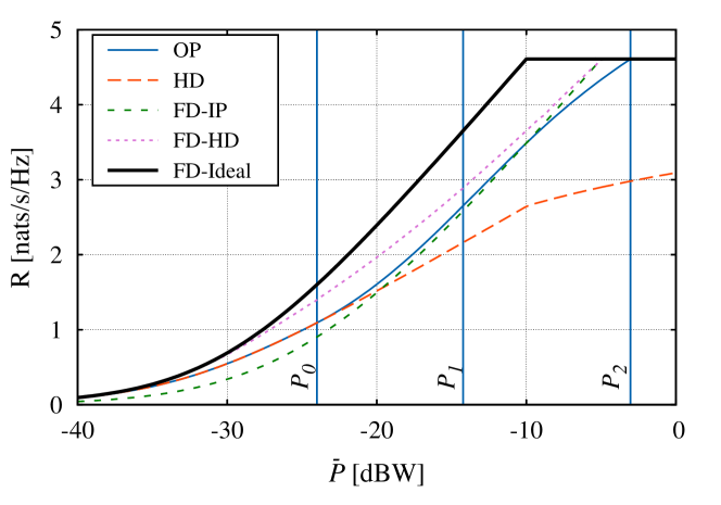
Figure 4: Achieved rate vs. $\bar{P}$, for $\bar{p}=-10$ dBW, $p^{\rm max}=-7$ dBW and $\beta=-135$ dB.

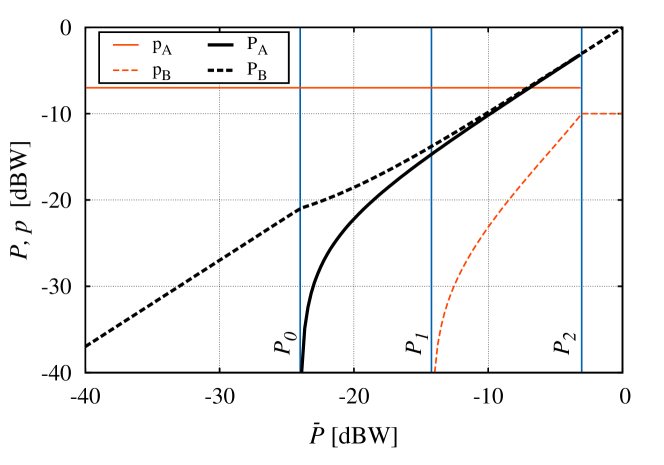
Figure 5: Optimal source and relay transmit power for phase A (solid lines) and phase B (dashed lines), for the same scenario as in Figure 4.

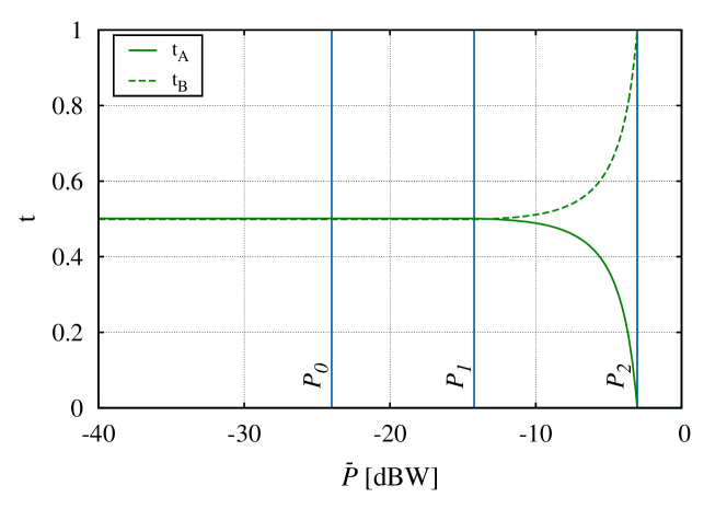
Figure 6: Phase durations $t_{A}$ (solid line) and $t_{B}$ (dashed line), for the same scenario as in Figure 4.

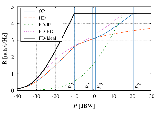
Figure 7: Achieved rate vs. $\bar{P}$, for $\bar{p}=-10$ dBW, $p^{\rm max}=-7$ dBW and $\beta=-110$ dB.

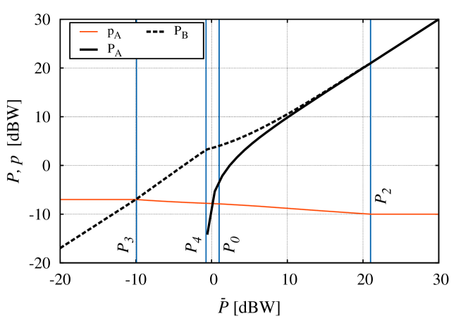
Figure 8: Optimal source and relay transmit power for phase A (solid lines) and phase B (dashed lines), for the same scenario as in Figure 7.

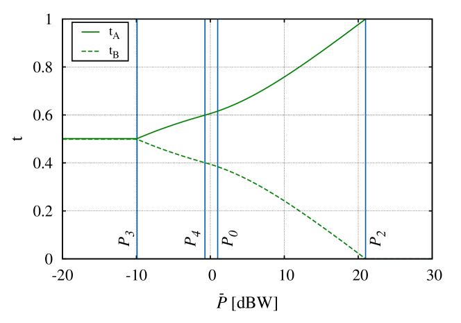
Figure 9: Phase durations $t_{A}$ (solid line) and $t_{B}$ (dashed line), for the same scenario as in Figure 7.

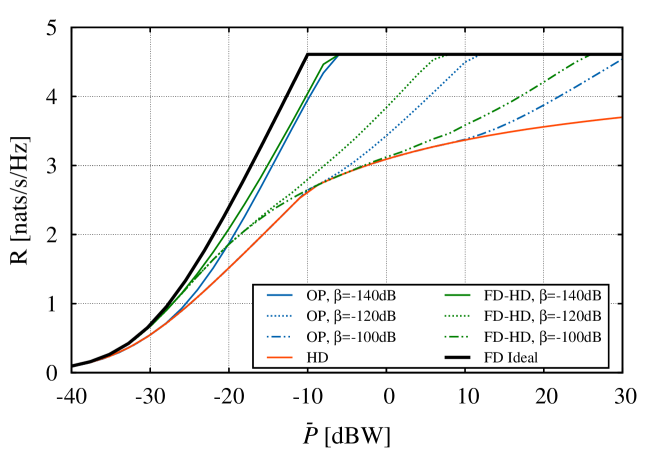
Figure 10: Achieved rate vs. $\bar{P}$, for $\bar{p}=-10$ dBW, $p^{\rm max}=-7$ dBW, and different values of $\beta$.

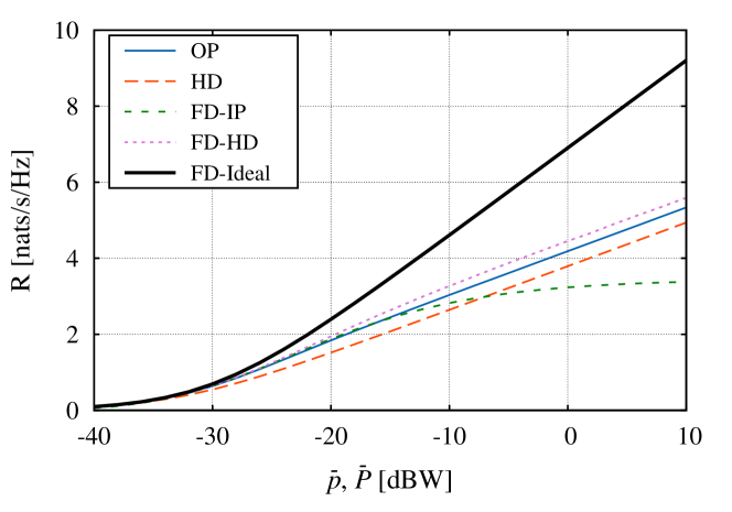
Figure 11: Achieved rate vs. $\bar{P}=\bar{p}$, for $p^{\rm max}=\bar{p}+3$ dB and $\beta=-130$ dB.

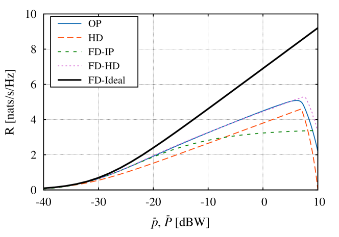
Figure 12: Achieved rate vs. $\bar{P}=\bar{p}$, for $p^{\rm max}=10$ dBW and $\beta=-130$ dB.

We compare the performance of our proposed scheme against the ideal full duplex communication scheme (in the following referred to as “FD Ideal”) where the relay does not suffer from self-interference. The expression of the corresponding rate is

$$R_{\rm FD-Ideal}=\min\left\{\log\left(1+\frac{\bar{P}|h_{1}|^{2}}{N_{0}}\right),\log\left(1+\frac{\bar{p}|h_{2}|^{2}}{N_{0}}\right)\right\}$$

which is also reported in [12, eq.(38)]. We then consider the full duplex scheme (referred to as “FD-IP”) where the source is aware of the instantaneous power (IP) at which the relay transmits. In FD-IP, the source always transmits with average power $\bar{P}$ while the relay transmits with average power $\bar{p}$. We stress that, unlike FD-IP, our scheme only requires the knowledge at the source of the average power used at the relay. The expression of the rate achieved by FD-IP is:

$$R_{\rm FD-IP} = \min\left\{\int_{-\infty}^{+\infty}\log\left(1+\frac{\bar{P}|h_{1}|^{2}}{N_{0}+\beta x^{2}}\right)\frac{{\rm e}^{-x^{2}/(2\bar{p})}}{\sqrt{2\pi\bar{p}}}{\rm\,d}x,\log\left(1+\frac{\bar{p}|h_{2}|^{2}}{N_{0}}\right)\right\}\,.$$ (42)

Furthermore, we compare our solution to the conventional half duplex scheme (named “HD”), for which the rate is given by

$$R_{\rm HD} = \max_{\bar{p}/p^{\rm max}\leq t\leq 1}\min\left\{(1\mathord{-}t)\log\left(1\mathord{+}\frac{|h_{1}|^{2}\bar{P}}{(1\mathord{-}t)N_{0}}\right),t\log\left(1+\frac{\bar{p}|h_{2}|^{2}}{tN_{0}}\right)\right\}$$ (43)

where the relay always operates in half duplex and its transmit power is limited to $p^{\rm max}$. This scheme implies that the communication is organized in two phases of duration $t$ and $1-t$, respectively.

Finally, we consider a hybrid communication scheme named FD-HD where the relay leverages on FD-IP or on HD, depending on which operational mode provides the highest rate. Specifically, FD-HD is organized in the following three phases: (A) the source transmits at power $P_{A}$ for a time fraction $t_{A}$ while the relay is silent; (B) the source is silent and the relay transmits at power $p_{B}$ for a time fraction $t_{B}$; (C) the relay operates in FD, source and relay transmit at power $P_{C}$ and $p_{C}$, respectively, for a time fraction $t_{C}$. As in FD-IP, the source has knowledge of the instantaneous power used by the relay. The achieved rate is given by:

$$R_{\rm FD-HD} = \max_{\begin{subarray}{c}t_{A},t_{B},t_{C}\\ P_{A},P_{C}\\ p_{B},p_{C}\end{subarray}}\min\left\{t_{A}\log\left(1+\frac{P_{A}|h_{1}|^{2}}{N_{0}}\right)+t_{C}\int_{-\infty}^{+\infty}\log\left(1+\frac{P_{C}|h_{1}|^{2}}{N_{0}+\beta x^{2}}\right)\frac{{\rm e}^{-x^{2}/(2p_{C})}}{\sqrt{2\pi p_{C}}}{\rm\,d}x,\right.$$ (44)

$$\left.t_{B}\log\left(1+\frac{p_{B}|h_{2}|^{2}}{N_{0}}\right)+t_{C}\log\left(1+\frac{p_{C}|h_{2}|^{2}}{N_{0}}\right)\right\}$$

where the first argument of the $\min$ operator represents the rate achieved on the source-relay link, the second one represents the rate achieved on the relay-destination link, and the following constraints must hold: $t_{A}+t_{B}+t_{C}=1$, $t_{A}P_{A}+t_{C}P_{C}=\bar{P}$, $t_{B}p_{B}+t_{C}p_{C}=\bar{p}$, and $p_{B},p_{C}\leq p^{\rm max}$.

In order to evaluate the performance of our solution against the above schemes, we consider a scenario similar to that employed in [12] where the source-relay and relay-destination distances are both set to $d=500$ m, the signal carrier frequency is $f_{c}=2.4$ GHz and the path loss is given by $|h_{1}|^{2}=|h_{2}|^{2}=\left(\frac{c}{4\pi f_{c}}\right)^{2}d^{-\alpha}$, with $\alpha=3$. Considering an additive noise with power spectral density -204 dBW/Hz and a bandwidth $B=200$ kHz, the noise power at both relay and destination receivers is about $N_{0}=-151$ dBW. Note that, for this setting, we have $v=|h_{1}|^{2}/N_{0}\approx 30$ dB.

Figure 4 compares the rate of our optimal power allocation scheme, labeled “OP”, against the performance of FD-Ideal, FD-IP, FD-HD and HD, for $\bar{p}=-10$ dBW, $p^{\rm max}=-7$ dBW and $\beta=-135$ dB. Since $\beta_{0}=\beta/N_{0}\approx 16$ dB, the results we derived for $v>\beta_{0}$ apply. Let $P_{i}={\cal P}_{i}\frac{\beta}{|h_{1}|^{2}}$, for $i=0,\ldots,4$. For the parameters used in this example, the value of the thresholds $P_{i}$ ($i=0,\ldots,4$) are: $P_{0}=-24$ dBW, $P_{1}=-14.23$ dBW, $P_{2}=-3.04$ dBW, $P_{3}=-9.92$ dBW, and $P_{4}=-20.56$ dBW. The thresholds $P_{3}$ and $P_{4}$ are meaningful only if lower than $P_{0}$ (see Section V), thus they are not shown in the figure. The achieved rates are depicted as functions of the average transmit power at the source, $\bar{P}$. For $\bar{P}\geq P_{0}$, the results obtained in Section IV hold. Accordingly, the plot highlights three operational regions corresponding to $P_{0}\leq\bar{P}\leq P_{1}$, $P_{1}<\bar{P}\leq P_{2}$, and $\bar{P}>P_{2}$, respectively. Instead, for $\bar{P}<P_{0}$ (see Section V), we have a single operational region only, since $P_{3}>P_{0}$ and $P_{4}>P_{0}$. We observe that all communication strategies are outperformed by FD-Ideal, which assumes no self-interference at the relay. Also, FD-HD outperforms both FD-IP and HD since it assumes perfect knowledge at the source about the instantaneous relay transmit power (as FD-IP) and can work in either FD or HD mode, depending on the system parameters. As far as our proposed technique is concerned, OP always outperforms HD and achieves higher rates than FD-IP for $\bar{P}<-10$ dBW. Furthermore, OP gets very close to FD-HD, especially for $\bar{P}>P_{1}$.

Such performance of the OP scheme is achieved for the source and relay transmit power levels and for the phase durations depicted in Figures 5 and 6, respectively. Interestingly, for $\bar{P}<P_{1}$, the time durations of the two communication phases remain constant. With regard to the transmit power, for $\bar{P}<P_{0}$, the source transmits in phase B and is silent in phase A while the relay only transmits in phase A at its maximum power. For $P_{0}\leq\bar{P}<P_{1}$, the source always transmits (even if at different power levels), while the relay only receives in phase B and transmits at its maximum power in phase A. For $P_{1}\leq\bar{P}<P_{2}$, both source and relay transmit but the duration of the two phases varies, with $t_{A}\to 0$ as $\bar{P}\to P_{2}$. Finally, for $\bar{P}\geq P_{2}$, both source and relay transmit at their average power level.

Figure 7 refers to the same scenario as that considered in Figure 4, but with the self-interference attenuation factor, $\beta$, set to -110 dB. In this case, $\beta_{0}=\beta/N_{0}\approx 41$ dB and the results obtained for $v<\beta_{0}$ apply. Moreover, we have: $P_{0}=1$ dBW, $P_{2}=21$ dBW, $P_{3}=-9.9$ dBW, and $P_{4}=-0.7$ dBW, while the threshold $P_{1}$ is negative (hence, it is not shown). The figure highlights two operational regions for $\bar{P}\geq P_{0}$ (namely, $P_{0}\leq\bar{P}\leq P_{2}$ and $\bar{P}\geq P_{2}$), and three operational regions for $\bar{P}<P_{0}$ (i.e., $\bar{P}<P_{3}$, $P_{3}\leq\bar{P}\leq P_{4}$ and $P_{4}<\bar{P}<P_{0}$). In this case too, OP outperforms FD-IP (except for high values of $\bar{P}$) and performs very close to FD-HD. By looking at Figure 8, which depicts the corresponding power levels used at source and relay, we note that in phase B the relay is always silent. In phase A, instead, the relay transmits at its maximum power (namely, -7 dBW) when $\bar{P}\leq P_{3}$, and it slowly decreases its power to $\bar{p}$ as $\bar{P}$ approaches $P_{2}$. With regard to the source, in phase B it always transmits for $\bar{P}<P_{2}$, although at different power levels depending on $\bar{P}$. On the contrary, in phase A it is silent for $\bar{P}<P_{4}$, and it always transmits for larger values of $\bar{P}$. These results match the values of the phase durations depicted in Figure 9: now, the region where the phase durations are constant is limited to $\bar{P}<P_{3}$, while, as $\bar{P}$ approaches $P_{2}$, $t_{A}\to 1$ and $t_{B}\to 0$.

Figure 10 highlights the impact of self-interference on the network performance. Indeed, the plot shows the rate versus $\bar{P}$, achieved by OP and its counterpart FD-HD, as $\beta$ varies. For sake of completeness, also the results for FD-Ideal and HD (which do not depend on $\beta$) are shown. For $\beta=-120$ dB (i.e., $v<\beta_{0}$), the system is affected by a substantial self-interference at the relay, and OP performs as HD for low-medium values of $\bar{P}$. As $\beta$ decreases (i.e., the effect of self-interference is smaller), the OP performance becomes closer to that of FD-HD and FD-Ideal; in particular, for $\beta=-140$ dB, the gap between OP and FD-HD reduces to about 1 dB.

In Figure 11, we study a different scenario where $\beta$ is fixed to -130 dB, $\bar{p}$ and $\bar{P}$ vary, and $p^{\rm max}=\bar{p}+3$ dB. Since now $\bar{P}$, $\bar{p}$ and $p^{\rm max}$ can all grow very large, the gap between FD-Ideal and all other schemes becomes much more evident. However, OP closely matches FD-HD and significantly outperforms HD. Interestingly, FD-IP provides a lower rate than HD as the transmit power at source and relay increases. This is because FD-IP cannot exploit the HD mode; thus, when $\bar{p}$ is large and the impact of self-interference becomes severe, there is no match with the other schemes.

Finally, Figure 12 addresses a similar scenario to the one above, but $p^{\rm max}$ is now fixed to 10 dBW. We observe that, as $\bar{p}$ grows, the rate provided by all schemes increases. However, when $\bar{p}$ approaches $p^{\rm max}$, the relay is constrained to transmit, i.e., to work in FD, for an increasingly longer time. For $\bar{p}=p^{\rm max}$, the relay always transmits at a power level equal to $\bar{p}=p^{\rm max}$. Also, the rate provided by the HD scheme drops to 0 while FD-IP and FD-HD provide the same performance; indeed, the latter cannot exploit anymore the advantages of HD. For the same reason, the OP scheme experiences a rate decrease. These results clearly suggest that significantly better performance can be achieved when $\bar{p}$ is not too close to $p^{\rm max}$.

VII Extension to finite $P^{\rm max}$

The analysis performed in Sections IV and V as well as the numerical results reported in Section VI have been obtained by assuming $P^{\rm max}$ to be very large. By relaxing this assumption, the transmission power at the source can be written as (see Appendix A):

$$P(p)=\min\left\{\frac{\beta}{|h_{1}|^{2}}[\omega-p]^{+},P^{\rm max}\right\}\,.$$ (45)

For simplicity, we define ${\cal P}^{\rm max}=\frac{|h_{1}|^{2}}{\beta}P^{\rm max}$ so that $P(p)$ can be more conveniently written as $P(p)=\frac{\beta}{|h_{1}|^{2}}{\cal P}(p)$ with ${\cal P}(p)=\min\left\{[\omega-p]^{+},{\cal P}^{\rm max}\right\}$.

Figure 13: Transmission power at the source, ${\cal P}(p)$, for ${\cal P}^{\rm max}\leq\omega$ (left) and ${\cal P}^{\rm max}>\omega$ (right).

The function ${\cal P}(p)$ is plotted in Figure 13 (blue line) for the cases ${\cal P}^{\rm max}\leq\omega$ (left) and ${\cal P}^{\rm max}>\omega$ (right).

The following cases can occur:

• ${\cal P}^{\rm max}>\omega$, then ${\cal P}(p)=[\omega-p]^{+}$. This leads to a situation similar to that considered in Sections IV and V. Indeed,

  • in Section IV, by imposing $\omega\geq p^{\rm max}$ in constraints (c), (d), and (e) of problem P1, we obtained $\omega=\bar{P}+\bar{p}$. It follows that $\bar{{\cal P}}$ should lie in the range $[p^{\rm max}-\bar{p},{\cal P}^{\rm max}-\bar{p}]$ where the results reported in Table I hold;

  • in Section V, we considered the case $\omega<p^{\rm max}$. Since ${\cal P}^{\rm max}>\omega$, we obtain $\omega<\min\{p^{\rm max},{\cal P}^{\rm max}\}$. If ${\cal P}^{\rm max}>p^{\rm max}$ the results shown in Table II hold, otherwise they need to be recomputed by simply considering $\omega$ ranging in $[0,{\cal P}^{\rm max})$.

• ${\cal P}^{\rm max}\leq\omega$, which is a more challenging scenario to analyse. Indeed, in such a situation function ${\cal P}(p)$, with $p\in[0,p^{\rm max}]$, takes values in up to three linear regions, depending on the value of $p^{\rm max}$. Specifically,

  • if $p^{\rm max}<\omega-{\cal P}^{\rm max}$, we have ${\cal P}(p)={\cal P}^{\rm max}$. Then the integral in (3) holds only if $\bar{{\cal P}}={\cal P}^{\rm max}$. This corresponds to the case where the source always transmits at its maximum power, regardless what the relay does;

  • if $\omega-{\cal P}^{\rm max}\leq p^{\rm max}<\omega$, ${\cal P}(p)$ takes values in two linear regions, i.e., ${\cal P}(p)={\cal P}^{\rm max}$ if $p\in[0,\omega-{\cal P}^{\rm max})$, and ${\cal P}(p)=\omega-p$ if $p\in[\omega-{\cal P}^{\rm max},p^{\rm max})$. In order to maximize the rate $R$ over the distribution $f(p)$, we then need to split it in two parts as done in Section V and the same analysis therein applies;

  • if $p^{\rm max}\geq\omega$ , ${\cal P}(p)$ is composed of three linear regions, i.e., ${\cal P}(p)={\cal P}^{\rm max}$ if $p\in[0,\omega-{\cal P}^{\rm max})$, ${\cal P}(p)=\omega-p$ if $p\in[\omega-{\cal P}^{\rm max},\omega)$, and ${\cal P}(p)=0$ otherwise. In this case, for any given $\omega$, the rate maximization problem can be solved by splitting $f(p)$ in three distributions having support in $[0,\omega-{\cal P}^{\rm max})$, $[\omega-{\cal P}^{\rm max},\omega)$, and $[\omega,p^{\rm max}]$, and having masses $F_{1}(\omega)$, $F_{2}(\omega)$, and $1-F_{1}(\omega)-F_{2}(\omega)$, respectively. The rate maximization can be performed following a procedure similar to that used in Section V, although in this case, we need to consider a three-dimensional (instead of a bi-dimensional) region $\Omega$, with coordinates $(\omega,F_{1},F_{2})$. Such maximization is quite cumbersome if performed analytically, but quite easy to solve numerically.

VIII Conclusions

We investigated the maximum achievable rate in dual-hop decode-and-forward networks where the relay can operate in full-duplex mode. Unlike existing work, in our scenario the source must be aware only of the distribution of the transmit power at the relay; under this assumption, we derived the allocation of the transmit power at the source and relay that maximize the data rate. Such distribution turned out to be discrete and composed of either one or two delta functions. This finding allowed us to identify the optimal network communication strategy, which, in general, is given by a two-phase time division scheme.

Our numerical results highlight the advantage of being able to gauge full-duplex and half-duplex at the relay, depending on the channel gains and the amount of self-interference affecting the system. They also underline the excellent performance of the proposed scheme, even when compared to strategies that assume the source to be aware of the instantaneous transmit power at the relay.

Appendix A Maximizing $R_{1}$ for a given $f(p)$

The optimization problem at hand is as follows:

$$\max\int_{0}^{p^{\rm max}}f(p)\log\left(1+\frac{P(p)|h_{1}|^{2}}{N_{0}+\beta p}\right){\rm\,d}p$$

$$s.t.$$

$$(a) \int_{0}^{p^{\rm max}}f(p)P(p){\rm\,d}p=\bar{P}$$

$$(b) 0\leq P(p)\leq P^{\rm max}$$

with $f(p)$ to be considered as a fixed arbitrary distribution.

We can solve the problem by writing Lagrange’s equation and leveraging the well-known Karush-Kuhn-Tucker (KKT) conditions. We define the Lagrangian as:

$${\cal L}(P) = f(p)\log\left(1+\frac{|h_{1}|^{2}}{N_{0}+\beta p}P(p)\right)-\lambda\left(f(p)P(p){\rm\,d}p-\bar{P}\right)$$ (46)

$$-\mu_{1}(p)(P(p)-P^{\rm max})+\mu_{2}(p)P(p)$$

where $\mu_{1}(p),\mu_{2}(p)\geq 0$ and $\lambda$ are the KKT multipliers. Writing the KKT conditions, we obtain:

$$\frac{|h_{1}|^{2}}{N_{0}+\beta p}\cdot\frac{f(p)}{1+\frac{P(p)|h_{1}|^{2}}{N_{0}+\beta p}}-\lambda f(p)-\mu_{1}(p)+\mu_{2}(p) = 0$$ (47)

$$\mu_{1}(p)(P(p)-P^{\rm max}) = 0$$ (48)

$$\mu_{2}(p)P(p) = 0$$ (49)

along with (a) and (b) that must still hold. It can be easily verified that the above system is satisfied when $\mu_{1}(p)=\mu_{2}(p)=0$, for which (47) reduces to:

$$f(p)\left[\frac{|h_{1}|^{2}}{N_{0}+\beta p}\cdot\frac{1}{1+\frac{P(p)|h_{1}|^{2}}{N_{0}+\beta p}}-\lambda\right]=0\,.$$ (50)

Excluding the trivial case where $f(p)=0$ $\forall p$ and taking into account the constraint $0\leq P(p)\leq P^{\rm max}$, we get the following expression for the optimal $P(p)$:

$$P(p)=\min\left\{\left[\frac{1}{\lambda}+\frac{N_{0}+\beta p}{|h_{1}|^{2}}\right]^{+},P^{\rm max}\right\}=\min\left\{\frac{\beta[\omega-p]^{+}}{|h_{1}|^{2}},P^{\rm max}\right\}$$ (51)

where we defined

$$\omega=\frac{|h_{1}|^{2}}{\beta\lambda}+\frac{N_{0}}{\beta}$$

which, in order to provide feasible solutions, must satisfy (a).

Appendix B

Lemma B.1

Let $\phi(p)$ be a continuous concave function in $p\in[a,b]$ and $f(p)$ be a probability distribution with support in $p\in[a,b]$ and average $\int_{a}^{b}pf(p){\rm\,d}p=m$. Then

$$p^{*}\phi(a)+(1-p^{*})\phi(b)\leq\int_{a}^{b}f(p)\phi(p){\rm\,d}p\leq\phi(m)$$

where $p^{*}=\frac{b-m}{b-a}$.

Proof:

The upper bound is obtained by applying Jensen inequality and holds with equality when $f(p)=\delta(p-m)$.

With regard to the lower bound, being $\phi(p)$ concave in $p\in[a,b]$, we can write

$$\phi(p)\geq\frac{\phi(b)-\phi(a)}{b-a}(p-a)+\phi(a)$$

Therefore,

$$\int_{a}^{b}f(p)\phi(p){\rm\,d}p \geq \int_{a}^{b}f(p)\left[\frac{\phi(b)-\phi(a)}{b-a}(p-a)+\phi(a)\right]{\rm\,d}p$$ (52)

$$= \frac{b-m}{b-a}\phi(a)+\left(1-\frac{b-m}{b-a}\right)\phi(b)\,.$$

The lower bound holds with equality when

$$f(p)=\frac{b-m}{b-a}\delta(p-a)+\left(1-\frac{b-m}{b-a}\right)\delta(p-b)\,.$$

∎

Appendix C Proof of Theorem IV.1

The calculus of variations problem in (IV.1) can be solved by using the Euler-Lagrange formula. To do so we first define the Lagrangian

$$L(z,f(p))=f(p)\phi(p)+\lambda_{1}f(p)\psi(p)+\lambda_{2}pf(p)+\lambda_{3}f(p)-\mu(p)f(p)$$

where the first term represents the functional to be minimized. The second, third and fourth terms represent the constraints (a), (b), and (c) with associated Lagrange multipliers $\lambda_{1}$, $\lambda_{2}$ and $\lambda_{3}$, respectively. As far as the last term is concerned, we first observe that constraint (d) can be rewritten as $-f(p)\leq 0$. In order to include (d) in the Lagrangian, we need to add a Lagrange multiplier for every $p\in[a,b]$. This can be done by introducing the multiplier $\mu(p)\geq 0$.

Next, we apply the Euler-Lagrange formula and we write the Karush-Kuhn-Tucker conditions associated with the problem. Specifically, we get

$$\frac{\partial L}{\partial f}=0\Rightarrow\mu(p)=\phi(p)+\lambda_{1}\psi(p)+\lambda_{2}p+\lambda_{3}$$

subject to the conditions (a), (b), (c), (d), $\mu(p)\geq 0$, and $\mu(p)f(p)=0$.

Now the key observation is that $\mu(p)=\phi(p)+\lambda_{1}\psi(p)+\lambda_{2}p+\lambda_{3}$ identifies a family of continuous functions driven by the parameters $\lambda_{1}$, $\lambda_{2}$ and $\lambda_{3}$. Such parameters need to be properly chosen in order to have $\mu(p)\geq 0,\forall p\in[a,b]$. If $\mu(p)$ is strictly positive in $[a,b]$ (i.e., $\mu(p)>0,\forall p\in[a,b]$), then the condition $\mu(p)f(p)=0$ implies $f(p)=0,\forall p\in[a,b]$, which is not a valid solution. Moreover, $\phi(p)$ and $\psi(p)$ are not constant functions, therefore it is not possible to find values of the Lagrange multipliers such that $\mu(p)=0$, in a subset of $[a,b]$ having non-zero measure. The only option is to allow $\mu(p)>0$ for all $p\in[a,b]$, except for a discrete set of points $p_{i}\in[a,b]$ for which $\mu(p_{i})=0$. This observation hints that the solution of the problem must be found in the set of discrete distributions. In practice, every solution $p_{i}$ of $\mu(p)=0$ is associated with a mass of probability, $\pi_{i}$, located at $p_{i}$.

The number of solutions of $\mu(p)=0$ can vary depending on the values of $\lambda_{1}$, $\lambda_{2}$, $\lambda_{3}$, $\gamma_{1}$, and $\gamma_{2}$. In general such a number can be computed by analyzing the first derivative of $\mu(p)$, i.e.,

$$\mu^{\prime}(p)=\frac{k_{1}p^{2}+k_{2}p+k_{3}}{(1+\gamma_{1}p)(1+\gamma_{2}p)}$$ (53)

where $k_{1},k_{2},k_{3}$ depend on $\lambda_{1}$, $\lambda_{2}$, $\lambda_{3}$, $\gamma_{1}$, $\gamma_{2}$.

The numerator of (53) is a polynomial in $p$ of degree 2 and thus has up to two solutions for $p$ in $[a,b]$, which correspond to local minima or maxima of $\mu(p)$.

Let $f^{\star}(p)$ be the minimizer of (IV.1). Then several cases are possible:

• $\mu(p)$ has a single solution $p_{1}\in[a,b]$ which does not correspond to local minima or maxima. Then $p_{1}=a$ or $p_{1}=b$. This implies $f^{\star}(p)=\pi_{1}\delta(p-a)$ (or, $f^{\star}(p)=\pi_{1}\delta(p-b)$) which, however has only one degree of freedom (i.e., the value of $\pi_{1}$) and thus, in general, cannot satisfy constraints (a), (b), and (c) of (IV.1) all together;

• $\mu(p)$ has a single solution $p_{1}\in[a,b]$ which corresponds to a local minimum. Thus $f^{\star}(p)=\pi_{1}\delta(p-p_{1})$. However, this solution is not feasible since it has only two degrees of freedom (i.e., $p_{1}$ and $\pi_{1}$) and therefore, in general, cannot satisfy the three constraints (a), (b), and (c) of (IV.1) at the same time;

• $\mu(p)$ has two solutions $p_{1},p_{2}\in[a,b]$ none of which corresponds to a local minimum. Thus $p_{1}=a$ and $p_{2}=b$, and $f^{\star}(p)=\pi_{1}\delta(p-a)+\pi_{2}\delta(p-b)$. Again, in general, this solution is not feasible since it has only two degrees of freedom ($\pi_{1}$ and $\pi_{2}$) and therefore cannot meet (a), (b), and (c) at the same time;

• $\mu(p)$ has two solutions $p_{1},p_{2}\in[a,b]$ one of which is a local minimum. Then two cases are possible, i.e., $\{p_{1}=a,p_{2}>a\}$ or $\{p_{1}<b,p_{2}=b\}$) and the minimizer $f^{\star}(p)$ takes the expression $f^{\star}(p)=\pi_{1}\delta(p-a)+\pi_{2}\delta(p-p_{2})$ or $f^{\star}(p)=\pi_{1}\delta(p-p_{1})+\pi_{2}\delta(p-b)$. This solution is feasible since it has three degrees of freedom represented by $\{\pi_{1},\pi_{2},p_{1}\}$ or $\{\pi_{1},\pi_{2},p_{2}\}$ that can be determined by imposing the constraints (a), (b), and (c). The constants $\gamma_{1}$, and $\gamma_{2}$ determine which of the two expressions in (14) is the minimizer. This is shown in Section C-A.

Since $\mu(p)$ cannot have more than two distinct solutions in $[a,b]$, (as it can be observed from the fact that $\mu^{\prime}(p)$ has at most two solutions), we conclude that the minimizer of (IV.1) is given by (14).

C-A Selecting the minimizer expression

As shown above, the minimizer can assume one of the two possible expressions reported in (14). Here we show that the choice of the minimizer depends on the parameters $\gamma_{1}$ and $\gamma_{2}$. To do so, we first observe that the family of distributions

$$f^{\star}(p,x,y)=\pi(x,y)\delta(p-x)+[1-\pi(x,y)]\delta(p-y)\,,$$ (54)

where

$$\pi(x,y)=\frac{y-m}{y-x}>0\,,$$

with $m\leq y\leq b$ and $a\leq x\leq m$, encompasses both expressions in (14). Specifically, the expressions reported in (14) are given by $f^{\star}(p,a,p_{2})$ and $f^{\star}(p,p_{1},b)$, respectively.

For the family of distributions in (54), constraint (c) in (IV.1) can be rewritten as

$$F(x,y) = \int_{a}^{b}f^{\star}(p,x,y)\psi(p){\rm\,d}p$$ (55)

$$= \pi(x,y)\psi(x)+[1-\pi(x,y)]\psi(y)$$

$$= c\,.$$

Similarly, the cost function, $\int_{a}^{b}f(p)\phi(p){\rm\,d}p$, can be written as

$$G(x,y)=\pi(x,y)\phi(x)+[1-\pi(x,y)]\phi(y)\,.$$

Observe that, since $\psi(p)=\phi(p)+\eta(p)$, we have $F(x,y)=G(x,y)+H(x,y)$ where

$$H(x,y)=\pi(x,y)\eta(x)+[1-\pi(x,y)]\eta(y)\,.$$

In the following, for the sake of notation simplicity, we drop the argument of the functions when not needed. We now make the following observations:

1. $F$ and $G$ are increasing functions of $x$ and decreasing functions of $y$. Indeed, for any concave function $\rho(p)$, $p\in[a,b]$ (as $\phi(p)$, $\eta(p)$ and $\psi(p)$) the partial derivative of $\pi\rho(x)+(1-\pi)\rho(y)$ is given by

   $$\frac{\partial[\pi\rho(x)+(1-\pi)\rho(y)]}{\partial x}=\frac{\pi}{y-x}\left(\rho^{\prime}(x)-\frac{\rho(y)-\rho(x)}{y-x}\right)>0\,.$$

   The factor $\pi/(y-x)$ is clearly positive since $\pi$ is positive by definition and $y>x$. Moreover, for a concave function, the difference quotient $\frac{\rho(y)-\rho(x)}{y-x}$ is smaller than the derivative of $\rho(p)$ computed in $x$. Similarly, it is straightforward to show that

   $$\frac{\partial[\pi\rho(x)+(1-\pi)\rho(y)]}{\partial y}<0\,;$$

2. the equation $F(x,y)=c$ is the implicit definition of the function $y_{c}(x)$, $a\leq x\leq p_{1}$ and $p_{2}\leq y\leq b$ with derivative defined as

   $$y_{c}^{\prime}(x)=\frac{{\rm\,d}y_{c}(x)}{{\rm\,d}x}=-\frac{\frac{\partial F}{\partial x}}{\frac{\partial F}{\partial y}}=-\frac{F_{x}}{F_{y}}\,,$$

   where, for simplicity, we defined $F_{x}=\frac{\partial F}{\partial x}$ and $F_{y}=\frac{\partial F}{\partial y}$. By the above arguments on the partial derivatives of $F$, we conclude that $y_{c}^{\prime}(x)>0$. Similarly, the function $G(x,y)=t$ is the implicit definition of the function $y_{t}(x)$ whose derivative $y_{t}^{\prime}(x)$ is positive.

3. Given the constant $c$, a value for $t$ exists such that $y_{c}(x)$ and $y_{t}(x)$ have a common solution $(x^{*},y^{*})$. For example, if $t=G(a,p_{2})$, the two curves share the point $(a,p_{2})$ where $p_{2}=y_{c}(a)$.

Now consider a value of $t$ such that the curves $y_{c}(x)$ and $y_{t}(x)$ intersect at point $P=(x^{*},y^{*})$, with $P\neq(a,p_{2}),P\neq(p_{1},b)$.

If $y_{c}^{\prime}(x)>y_{t}^{\prime}(x)$ at $P$ then $t$ is not the global minimum of the cost function in (IV.1). Indeed, it exists $\epsilon>0$ such that the curve $y_{t-\epsilon}(x)$ intersects $y_{c}(x)$ at some point $P^{\prime}=(x^{*}+\Delta_{x},y^{*}+\Delta_{y})$ where the cost function $G(x^{*}+\Delta_{x},y^{*}+\Delta_{y})=t-\epsilon$ is clearly lower than at $P$. Since this is true for any point $P=(x^{*},y^{*})$ we conclude that the minimizer is $f^{\star}(p,p_{1},b)$ and that the minimum is thus $G(p_{1},b)$. By applying similar arguments, if $y_{c}^{\prime}(x)<y_{t}^{\prime}(x)$ at $P$ the minimizer is $f^{\star}(p,a,p_{2})$ and the minimum is $G(a,p_{2})$.

In order to compare the derivatives of $y_{c}^{\prime}(x)$ and $y_{t}^{\prime}(x)$ we use the definitions of $F$, $G$, and $H$ and write the following differential equations

$$y_{c}^{\prime}(x)=-\frac{F_{x}}{F_{y}}=-\frac{G_{x}+H_{x}}{G_{y}+H_{y}}\,,\hskip 17.22217pty_{t}^{\prime}(x)=-\frac{G_{x}}{G_{y}}$$

where $G_{x}$, $H_{x}$, $G_{y}$, $H_{y}$ are the partial derivatives of $G$ and $H$ w.r.t. $x$ and $y$, respectively. By considering $y_{c}^{\prime}(x)\geq y_{t}^{\prime}(x)$, we obtain

$$-\frac{G_{x}+H_{x}}{G_{y}+H_{y}}\geq-\frac{G_{x}}{G_{y}}\Rightarrow-\frac{G_{x}}{G_{y}}\leq-\frac{H_{x}}{H_{y}}\,.$$

We also observe that

$$\frac{\partial\pi}{\partial x}=\pi_{x}=\frac{\pi}{y-x}\,;\hskip 25.83325pt\frac{\partial\pi}{\partial y}=\pi_{y}=\frac{1-\pi}{y-x}\,.$$

Therefore, we have

$$G_{x} = \pi_{x}\phi(x)+\pi\phi^{\prime}(x)-\pi_{x}\phi(y)=\pi\left[\phi^{\prime}(x)-\frac{\phi(y)-\phi(x)}{y-x}\right]$$

$$G_{y} = \pi_{y}\phi(x)-\pi_{y}\phi(y)+(1-\pi)\phi^{\prime}(y)=(1-\pi)\left[\phi^{\prime}(y)-\frac{\phi(y)-\phi(x)}{y-x}\right]$$

$$H_{x} = \pi_{x}\eta(x)+\pi\eta^{\prime}(x)-\pi_{x}\eta(y)=\pi\left[\eta^{\prime}(x)-\frac{\eta(y)-\eta(x)}{y-x}\right]$$

$$H_{y} = \pi_{y}\eta(x)-\pi_{y}\eta(y)+(1-\pi)\eta^{\prime}(y)=(1-\pi)\left[\eta^{\prime}(y)-\frac{\eta(y)-\eta(x)}{y-x}\right]\,.$$

Now observe that $\phi(p)=\log(1+\gamma_{1}p)$ and $\eta(p)=\log(1+\gamma_{2}p)$ are the same function (i.e., $\log(1+\gamma p)$), the former evaluated in $\gamma=\gamma_{1}$ and the latter in $\gamma=\gamma_{2}$. Therefore, since $G$ depends on $\phi(p)$ and $H$ depends on $\eta(p)$, we can write $-\frac{G_{x}}{G_{y}}=\zeta(\gamma_{1})$ and $-\frac{H_{x}}{H_{y}}=\zeta(\gamma_{2})$.

It is easy to show that $\zeta(\gamma)$ increases with $\gamma$; indeed, by imposing $\zeta^{\prime}(\gamma)\geq 0$, after some algebra and after simplifying positive factors, we obtain

$$\log\left(\frac{1+\gamma y}{1+\gamma x}\right)(2+\gamma y+\gamma x)\geq 2\gamma(y-x)\,.$$

The right hand side (r.h.s.) of the previous inequality is positive and linear with $\gamma$, $\gamma\geq 0$. The left hand side (l.h.s.) is positive, convex and tangent to the r.h.s. at $\gamma=0$. Therefore, the above inequality always holds and $\zeta(\gamma)$ increases with $\gamma$. We conclude that if $\gamma_{1}<\gamma_{2}$, we have $-\frac{G_{x}}{G_{y}}\leq-\frac{H_{x}}{H_{y}}$ and, thus, $y_{c}(x)>y_{t}(x)$. In such a case the minimizer is $f^{\star}(p,p_{1},b)$. Similarly, when $\gamma_{1}>\gamma_{2}$, the minimizer is $f^{\star}(p,a,p_{2})$.

Appendix D Behavior of the curve $Q_{1}(\omega,F)=0$

The curve $Q_{1}(\omega,F)$ intersects the line $\omega=\bar{p}+\bar{{\cal P}}$ at most in a single point. To prove this, we substitute $\omega=\bar{p}+\bar{{\cal P}}$ in the expression for $Q_{1}(\omega,F)=0$, i.e., we compute $(R_{1}^{\rm min}=\widetilde{R}_{2}^{\rm max})|_{\omega=\bar{p}+\bar{{\cal P}}}$. After some algebra and by setting $a=\beta_{0}(\bar{p}+\bar{{\cal P}})$, we obtain:

$$-\log\left(1-\frac{\bar{{\cal P}}\beta_{0}}{F(1+a)}\right)=F\log\left(1-\frac{\bar{{\cal P}}\beta_{0}v}{F(\beta_{0}+av)}\right)+\log\left(1+\frac{av}{\beta_{0}}\right)\,.$$ (57)

Observe that the l.h.s of (57) is defined when $\frac{\bar{{\cal P}}\beta_{0}}{F(1+a)}<1$, i.e., when $F\geq\frac{\bar{{\cal P}}\beta_{0}}{1+a}$, which is always true since in $\Omega$ $F$ is larger that the value it achieves in $V_{3}$, i.e., $\frac{\bar{{\cal P}}\beta_{0}}{a}$. Moreover, the l.h.s of (57) decreases with $F$ while the r.h.s of (57) increases with $F$; thus, (57) has at most one solution.

Appendix E Behavior of $R_{1}^{\rm min}$,$R_{1}^{\rm max}$, $R_{2}^{\rm min}$,$R_{2}^{\rm max}$

E-A $R_{1}^{\rm min}$

We first observe that $R_{1}^{\rm min}$ can be rewritten as

$$R_{1}^{\rm min}=F\log\left(1+\frac{\bar{{\cal P}}\beta_{0}}{F(1+\omega\beta_{0})-\bar{{\cal P}}\beta_{0}}\right)\,.$$

From the above expression, we immediately observe that $R_{1}^{\rm min}$ decreases with $\omega$. We then compute the partial derivative of $R_{1}^{\rm min}$ w.r.t. $F$. We have

$$\frac{\partial}{\partial F}R_{1}^{\rm min}=\log\left(1+\frac{a}{F-a}\right)-\frac{a}{F-a}$$

where $a=\bar{{\cal P}}\beta_{0}/(1+\omega\beta_{0})$. Then $\frac{\partial}{\partial F}R_{1}^{\rm min}\leq 0$ implies

$$\log\left(1+\frac{a}{F-a}\right)\leq\frac{a}{F-a}\,.$$

Since $\log(1+y)\leq y$, for $y>-1$, we conclude that $R_{1}^{\rm min}$ decreases with $F$.

E-B $R_{1}^{\rm max}$

$R_{1}^{\rm max}$ does not depend on $F$; moreover,

$$\frac{\partial}{\partial\omega}R_{1}^{\rm max}=-\bar{{\cal P}}\frac{(1+\beta_{0}\omega)\log(1+\beta_{0}\omega)-\beta_{0}\omega}{\omega^{2}(1+\beta_{0}\omega)}\,.$$

Therefore, $\frac{\partial}{\partial\omega}R_{1}^{\rm max}\leq 0$ implies $(1+\beta_{0}\omega)\log(1+\beta_{0}\omega)>\beta_{0}\omega$, which is always true since $\beta_{0}\omega\geq 0$ and $y\leq(1+y)\log(1+y)$ for $y\geq 0$. Hence, $R_{1}^{\rm max}$ decreases with $\omega$.

E-C $R_{2}^{\rm min}$

We now consider the expression for $\widetilde{R}_{2}^{\rm min}$ reported in (35), which can be rewritten as

$$\widetilde{R}_{2}^{\rm min}=(1-F)\log\left(1+\frac{a}{1-F}\right)+c$$

where $a>0$ and $c$ do not depend on $F$. Now

$$\frac{\partial}{\partial F}\widetilde{R}_{2}^{\rm min}=\frac{\frac{a}{1-F}}{1+\frac{a}{1-F}}-\log\left(1+\frac{a}{1-F}\right)\,.$$

Thus, $\frac{\partial}{\partial F}\widetilde{R}_{2}^{\rm min}\leq 0$ implies

$$\frac{a}{1-F}\leq\left(1+\frac{a}{1-F}\right)\log\left(1+\frac{a}{1-F}\right)\,.$$

Since $y\leq(1+y)\log(1+y)$ for $y>0$, the above statement is true; hence, $\widetilde{R}_{2}^{\rm min}$ decreases with $F$.

We now consider the partial derivative w.r.t. $\omega$:

$$\frac{\partial}{\partial\omega}\widetilde{R}_{2}^{\rm min}=\frac{\bar{{\cal P}}}{\omega^{2}}\log(1+\omega v)+v\frac{\left(F-\frac{\bar{{\cal P}}}{\omega}\right)}{1+\omega v}-\frac{vF}{1+\omega v+v\frac{\bar{p}+\bar{{\cal P}}-\omega}{1-F}}\,.$$

We observe that the arguments of the logarithms are always positive. Moreover, the last term is negative since $F>0$ and $\bar{p}+\bar{{\cal P}}\geq\omega$, while the second term is positive since $F\geq\frac{\bar{{\cal P}}}{\omega}$. We now make the following key observation about the last term:

$$\frac{vF}{1+\omega v+v\frac{\bar{p}+\bar{{\cal P}}-\omega}{1-F}}\leq\frac{vF}{1+\omega v}\,.$$

Thus,

$$\frac{\partial}{\partial\omega}\widetilde{R}_{2}^{\rm min} \geq \frac{\bar{{\cal P}}}{\omega^{2}}\log(1+\omega v)+v\frac{F-\frac{\bar{{\cal P}}}{\omega}}{1+\omega v}-\frac{vF}{1+\omega v}$$ (58)

$$= \frac{\bar{{\cal P}}}{\omega^{2}}\log(1+\omega v)-\frac{\bar{{\cal P}}v}{\omega(1+\omega v)}$$

which is positive since $(1+\omega v)\log(1+\omega v)\geq\omega v$. It follows that $\widetilde{R}_{2}^{\rm min}$ increases with $\omega$.

E-D $R_{2}^{\rm max}$

By deriving $\widetilde{R}_{2}^{\rm max}$ in (35) w.r.t. $\omega$, we get

$$\frac{\partial}{\partial\omega}\widetilde{R}_{2}^{\rm max}=\frac{(F\bar{p}-\omega F+\bar{{\cal P}})v^{2}}{(1-F)\left(1+v\frac{\bar{p}+\bar{{\cal P}}-\omega F}{1-F}\right)\left(1+v\left(\omega-\frac{\bar{{\cal P}}}{F}\right)\right)}\,.$$

Since the arguments of the logarithms are positive, so is the denominator. Therefore, by imposing $\frac{\partial}{\partial\omega}\widetilde{R}_{2}^{\rm max}\geq 0$ and solving for $\omega$, we get $\omega\leq\bar{p}+\frac{\bar{{\cal P}}}{F}$. Since $F<1$, then $\bar{p}+\frac{\bar{{\cal P}}}{F}\geq\bar{p}+\bar{{\cal P}}$. Since in the region $\Omega$ we have $\omega\leq\bar{p}+\bar{{\cal P}}$, we conclude that $\widetilde{R}_{2}^{\rm max}$ increases with $\omega$.

Appendix F Maximizing the rate over subregion $\Omega_{3}$

• For $v\geq\beta_{0}$, according to Theorem IV.1, the function $g(p)$ for which P4 is maximized is given by

  $$g(p)=\frac{\frac{\bar{{\cal P}}}{F}}{\omega-p_{1}}\delta(p-p_{1})+\left(1-\frac{\frac{\bar{{\cal P}}}{F}}{\omega-p_{1}}\right)\delta(p-\omega)\,.$$ (59)

  Substituting this expression in (38), we can rewrite the problem as:

  $$R_{\Omega_{3}} = \max_{(\omega,F)\in\Omega_{3}}\frac{\bar{{\cal P}}}{\omega-p_{1}}\log\left(\frac{1+\beta_{0}\omega}{1+\beta_{0}p_{1}}\right)$$ (62)

  $${\rm s.t.}$$

  $$\frac{\bar{{\cal P}}}{\omega-p_{1}}\log\left[\frac{(1+\beta_{0}p_{1})(1+vp_{1})}{(1+\beta_{0}\omega)(1+v\omega)}\right]=C_{1}(\omega,F)$$

  $$C_{1}(\omega,F)=FC(\omega,F)-F\log\left[(1+\beta_{0}\omega)(1+v\omega)\right]\,.$$

  We first observe that the argument of (62) decreases with $p_{1}$. Indeed,

  $$\frac{\partial}{\partial p_{1}}\frac{\log\left(\frac{1+\beta_{0}\omega}{1+\beta_{0}p_{1}}\right)}{\omega-p_{1}} = \frac{1}{(\omega-p_{1})^{2}}\left[\log\left(\frac{1+\beta_{0}\omega}{1+\beta_{0}p_{1}}\right)-\frac{\beta_{0}(\omega-p_{1})}{1+\beta_{0}p_{1}}\right]$$ (63)

  $$\leq \frac{1}{(\omega-p_{1})^{2}}\left[\frac{1+\beta_{0}\omega}{1+\beta_{0}p_{1}}-1-\frac{\beta_{0}(\omega-p_{1})}{1+\beta_{0}p_{1}}\right]$$

  $$= 0$$

  where we used the bound $\log y\leq y-1$.

  Also, the l.h.s. of (62) increases with $p_{1}$. This can be easily seen considering that, if we let $\zeta(p)=\frac{(1+\beta_{0}p)(1+vp)}{(1+\beta_{0}\omega)(1+v\omega)}>0$, we can write

  $$\frac{\partial}{\partial p}\frac{\log\zeta(p)}{\omega-p}=\frac{\zeta^{\prime}(p)}{\zeta(p)(\omega-p)}+\frac{\log\zeta(p)}{(\omega-p)^{2}}=\frac{\zeta^{\prime}(p)(\omega-p)+\zeta(p)\log\zeta(p)}{\zeta(p)(\omega-p)^{2}}\,.$$ (64)

  Note that the denominator of the above equation is positive. Now $\zeta(p)=\zeta_{1}(p)\zeta_{2}(p)$ where $\zeta_{1}(p)=\frac{1+\beta_{0}p}{1+\beta_{0}\omega}$ and $\zeta_{2}(p)=\frac{1+vp}{1+v\omega}$. It follows that the numerator of (64) can be rewritten as

  $$\zeta^{\prime}(p)(\omega-p)+\zeta(p)\log\zeta(p) = \zeta^{\prime}(p)(\omega-p)+\zeta_{2}(p)\zeta_{1}(p)\log\zeta_{1}(p)+\zeta_{1}(p)\zeta_{2}(p)\log\zeta_{2}(p)$$ (65)

  $$\geq \zeta^{\prime}(p)(\omega-p)+\zeta_{2}(p)[\zeta_{1}(p)-1]+\zeta_{1}(p)[\zeta_{2}(p)-1]$$

  $$= \zeta^{\prime}(p)(\omega-p)+2\zeta(p)-\zeta_{1}(p)-\zeta_{2}(p)$$

  $$= 0$$

  where we used the bound $y\log y\geq y-1$ which holds for any $y>0$. With regard to $C_{1}(\omega,F)$, we consider the curves $Q_{2}(\omega,F)=t$ where $t<0$ is a parameter. Note that such curves are located on the left of $Q_{2}(\omega,F)=0$. By definition of $Q_{2}(\omega,F)$, we have

  $$Q_{2}(\omega,F) = \widetilde{R}_{2}^{\rm min}-R_{1}^{\rm max}$$ (66)

  $$= \left(F-\frac{\bar{{\cal P}}}{\omega}\right)\log(1+v\omega)+(1-F)\log\left(1+v\frac{\bar{{\cal P}}+\bar{p}-F\omega}{1-F}\right)$$

  $$\qquad-\frac{\bar{{\cal P}}}{\omega}\log(1+\beta_{0}\omega)$$

  $$= \left(F-\frac{\bar{{\cal P}}}{\omega}\right)\log\left[(1+\beta_{0}\omega)(1+v\omega)\right]-FC(\omega,F)$$

  $$= t\,.$$

  Therefore, the term $C_{1,t}(\omega,F)$ defined in (62) can be written as

  $$C_{1,t}(\omega,F)=-t-\frac{\bar{{\cal P}}}{\omega}\log\left[(1+\beta_{0}\omega)(1+v\omega)\right]\,.$$

  The subscript $t$ indicates that we are restricting our analysis to the curve $Q_{2}(\omega,F)=t$. Observe that the expression for $C_{1,t}(\omega,F)$ does not depend on $F$; thus, as $t$ increases, $C_{1,t}(\omega,F)$ decreases. Since the l.h.s. of (62) increases with $p_{1}$, the value of $p_{1}$ for which the constraint is met decreases as $t$ increases. Finally, since the argument of (62) decreases with $p_{1}$, we conclude that the rate increases as $t$ increases.

  Since the curves $Q_{2}(\omega,F)=t$ have positive derivative in the $(\omega,F)$ plane, and as $t$ increases they move to the right, then, for any fixed $\hat{\omega}$, the solution for $F$ of $Q_{2}(\hat{\omega},F)=t$ decreases as $t$ increases. It follows that the rate $R_{\Omega_{3}}$ is achieved on curve $B$–$D$ as well. Thus, $R=R_{\Omega_{1}}=R_{\Omega_{3}}$ and $R$ can be computed by solving $R=\max_{Q_{1}(\omega,F)=0}R_{1}^{\rm min}$.

• For $v<\beta_{0}$, according to Theorem IV.1, $g(p)$ of P4 is given by

  $$g(p)=\frac{p_{2}-\omega+\frac{\bar{{\cal P}}}{F}}{p_{2}}\delta(p)+\frac{\omega-\frac{\bar{{\cal P}}}{F}}{p_{2}}\delta(p-p_{2})\,.$$ (67)

  Replacing $g(p)$ in (38) with the above expression, we get

  $$R_{\Omega_{3}}=\max_{(\omega,F)\in\Omega_{3}}F\log(1+\beta_{0}\omega)+\frac{\bar{{\cal P}}-F\omega}{p_{2}}\log(1+\beta_{0}p_{2})$$ (68)

  under the constraint

  $$\frac{\log\left[(1+\beta_{0}p_{2})(1+vp_{2})\right]}{p_{2}} = \frac{\log(1+\beta_{0}\omega)+\left(1-\frac{1}{F}\right)\log\left(1+v\frac{\bar{{\cal P}}+\bar{p}-F\omega}{1-F}\right)}{\omega-\frac{\bar{{\cal P}}}{F}}\,.$$ (69)

  In this case, an analytic solution of the optimization problem cannot be easily obtained since the involved terms do not exhibit the monotonic behavior observed above. By solving the problem numerically, it turns out that the optimum is located in $A=(\omega_{A},F_{A})$ for ${\cal P}_{3}\leq\bar{{\cal P}}\leq{\cal P}_{4}$, and in $V_{2}=(\bar{{\cal P}}+\bar{p},1)$ for ${\cal P}_{4}\leq\bar{{\cal P}}\leq{\cal P}_{2}$.

References

- [1] A. E. Gamal, M. Mohseni, and S. Zahedi, “Bounds on capacity and minimum energy-per-bit for awgn relay channels,” IEEE Transactions on Information Theory, vol. 52, no. 4, pp. 1545–1561, April 2006.
- [2] A. Zafar, M. Shaqfeh, M. S. Alouini, and H. Alnuweiri, “Resource allocation for two source-destination pairs sharing a single relay with a buffer,” IEEE Transactions on Communications, vol. 62, no. 5, pp. 1444–1457, May 2014.
- [3] M. Cardone, D. Tuninetti, R. Knopp, and U. Salim, “On the gaussian half-duplex relay channel,” IEEE Transactions on Information Theory, vol. 60, no. 5, pp. 2542–2562, May 2014.
- [4] R. R. Thomas, M. Cardone, R. Knopp, D. Tuninetti, and B. T. Maharaj, “A practical feasibility study of a novel strategy for the gaussian half-duplex relay channel,” IEEE Transactions on Wireless Communications, vol. 16, no. 1, pp. 101–116, Jan 2017.
- [5] L. Wang and M. Naghshvar, “On the capacity of the noncausal relay channel,” IEEE Transactions on Information Theory, vol. 63, no. 6, pp. 3554–3564, June 2017.
- [6] G. Kramer, “Models and theory for relay channels with receive constraints,” in Proc. 42nd Annu. Allerton Conf. Commun., Control, Comput., September 2004, p. 1312–1321.
- [7] N. Zlatanov, V. Jamali, and R. Schober, “On the capacity of the two-hop half-duplex relay channel,” in 2015 IEEE Global Communications Conference (GLOBECOM), Dec 2015, pp. 1–7.
- [8] T. Riihonen, S. Werner, and R. Wichman, “Hybrid full-duplex/half-duplex relaying with transmit power adaptation,” IEEE Transactions on Wireless Communications, vol. 10, no. 9, pp. 3074–3085, September 2011.
- [9] B. P. Day, A. R. Margetts, D. W. Bliss, and P. Schniter, “Full-duplex mimo relaying: Achievable rates under limited dynamic range,” IEEE Journal on Selected Areas in Communications, vol. 30, no. 8, pp. 1541–1553, September 2012.
- [10] Y. Y. Kang, B. J. Kwak, and J. H. Cho, “An optimal full-duplex af relay for joint analog and digital domain self-interference cancellation,” IEEE Transactions on Communications, vol. 62, no. 8, pp. 2758–2772, Aug 2014.
- [11] A. Behboodi, A. Chaaban, R. Mathar, and M. S. Alouini, “On full duplex gaussian relay channels with self-interference,” in 2016 IEEE International Symposium on Information Theory (ISIT), July 2016, pp. 1864–1868.
- [12] N. Zlatanov, E. Sippel, V. Jamali, and R. Schober, “Capacity of the gaussian two-hop full-duplex relay channel with residual self-interference,” IEEE Transactions on Communications, vol. 65, no. 3, pp. 1005–1021, March 2017.
- [13] T. Cover and A. E. Gamal, “Capacity theorems for the relay channel,” IEEE Transactions on Information Theory, vol. 25, no. 5, pp. 572–584, September 1979.
- [14] T. Riihonen, S. Werner, and R. Wichman, “Mitigation of loopback self-interference in full-duplex mimo relays,” IEEE Transactions on Signal Processing, vol. 59, no. 12, pp. 5983–5993, Dec 2011.
- [15] D. Korpi, T. Riihonen, K. Haneda, K. Yamamoto, and M. Valkama, “Achievable transmission rates and self-interference channel estimation in hybrid full-duplex/half-duplex mimo relaying,” in 2015 IEEE 82nd Vehicular Technology Conference (VTC2015-Fall), Sept 2015, pp. 1–5.
- [16] C. Y. A. Shang, P. J. Smith, G. K. Woodward, and H. A. Suraweera, “Linear transceivers for full duplex mimo relays,” in 2014 Australian Communications Theory Workshop (AusCTW), Feb 2014, pp. 11–16.
- [17] Q. Shi, M. Hong, X. Gao, E. Song, Y. Cai, and W. Xu, “Joint source-relay design for full-duplex mimo af relay systems,” IEEE Transactions on Signal Processing, vol. 64, no. 23, pp. 6118–6131, Dec 2016.