Optimal Throughput Fairness Trade-offs for Downlink Non-Orthogonal Multiple Access over Fading Channels

Abstract

Recently, non-orthogonal multiple access (NOMA) has attracted considerable interest as one of the 5G-enabling techniques. However, users with better channel conditions in downlink communications intrinsically benefits from NOMA thanks to successive decoding, judicious designs are required to guarantee user fairness. In this paper, a two-user downlink NOMA system over fading channels is considered. For delay-tolerant transmission, the average sum-rate is maximized subject to both average and peak power constraints as well as a minimum average user rate constraint. The optimal resource allocation is obtained using Lagrangian dual decomposition under full channel state information at the transmitter (CSIT), while an effective power allocation policy under partial CSIT is also developed based on analytical results. In parallel, for delay-limited transmission, the sum of delay-limited throughput (DLT) is maximized subject to a maximum allowable user outage constraint under full CSIT, and the analysis for the sum of DLT is also performed under partial CSIT. Furthermore, an optimal orthogonal multiple access (OMA) scheme is also studied as a benchmark to prove the superiority of NOMA over OMA under full CSIT. Finally, the theoretical analysis is verified by simulations via different trade-offs for the average sum-rate (sum-DLT) versus the minimum (maximum) average user rate (outage) requirement.

I Introduction

As the incoming fifth generation (5G) wireless communications features massive connectivity among heterogeneous types of users in the Internet of Things (IoT), non-orthogonal multiple access (NOMA) has been envisioned as a promising candidate for 5G networks [2, 3, 4], due to its advantage in enabling high spectral efficiency via non-orthogonal resource allocations over other orthogonal multiple access (OMA) techniques, such as time-division multiple access (TDMA) and frequency-division multiple access (FDMA) (see [5] and the references therein). Hence, it has recently sparked widespread interest in both industry [6, 7] and academia [8, 9, 10, 11, 12, 13, 14, 15, 16, 17]. Variation forms of NOMA, namely, multi-user superposition transmission (MUST) and layer division multiplexing (LDM), have been included in the 3rd Generation Partnership Project Long Term Evolution Advanced (3GPP-LTE-A) [6] and the next general digital TV standard ATSC 3.0 [7], respectively.

Among a variety of studies addressing the challenges posed by NOMA, a general NOMA downlink framework was proposed in [8] in which a base station (BS) is capable of simultaneously communicating with several randomly deployed users. To increase the throughput of cell-edge users in multi-cell NOMA networks, coordinated multi-point (CoMP) transmission techniques were adopted in [9] and [10] with the BS equipped with a single antenna and multiple antennas, respectively.

On another front, far users that suffer from severe path-loss attenuation are usually disadvantaged in competing for resources enhancing the sum throughput of the system, and therefore their performance could be substantially compromised without proper design. Multi-user proportional fairness was adopted in [2] as a scheduling metric to achieve a good trade-off between system throughput and user fairness. There are mainly three types of countermeasures against such unfairness in NOMA networks. The first strategy is to invoke cooperative NOMA [11, 12], in which a nearby user is regarded as a relay to assist a distant user. It is demonstrated in [11] that by utilizing the proposed cooperative protocol, all users experience the same diversity order. In [12] the nearby NOMA users are equipped with wireless energy harvesting capability to assist far users. The second strategy is to enhance the worst user performance [13, 14, 15]. The max-min power allocation problem that maximizes the minimum achievable user rate was studied for single-input-single-output (SISO) NOMA systems in [13], and for clustered multiple-input-multiple-output (MIMO) NOMA systems in [14]. In [15], the authors provided a mathematical proof for NOMA’s superiority over conventional OMA transmission in terms of the optimum sum rate subject to a minimum rate constraint. The third strategy is to introduce additional factors to guarantee fairness. Weighted sum-rate is an effective metric to reflect the priority of users in resource allocation [16, 17]. [16] considered a mutli-carrier downlink network, in which each sub-channel can be shared by multiple users by adopting NOMA. Joint sub-channel and power allocation was formulated as a weighted sum-rate maximization problem, and iteratively solved by leveraging a matching problem with externalities. multi-carrier NOMA systems employing a full-dupex (FD) BS was considered in [17], and an optimal joint sub-carrier and power policy for maximizing the weighted sum-rate was developed by applying monotonic optimization.

I-A Related Work

Fairness issues were studied for NOMA over fading channels in the above work. However, they were either considered in a long term with fixed power allocations, e.g., in [8, 12], or investigated exploiting adaptive allocation of power and/or bandwidth in a short term, e.g., in [16, 17]. By contrast, we consider adaptive resource allocations to channel dynamics for a two-user downlink NOMA over the whole fading process, the system design of which requires satisfying long-term constraints for quality-of-service (QoS) thus posing new challenges compared with short-term objectives. The information theoretic study of fading broadcast channels (BCs) can be traced back to [18] and [19]. Assuming perfect channel state information (CSI) at both the transmitter (Tx) and the receivers (Rxs), dynamic power and rate allocations for various transmission schemes including code division (CD) with and without successive decoding, time division, and frequency division over different fading states were studied for the ergodic capacity region (ECR) and the (zero-) outage capacity region (OCR) in [18] and [19], respectively. The boundaries of the ECRs have been characterized in [18] by solving equivalent weighted sum-rate problems each corresponding to one set of weights. The (zero-) OCRs were inexplicitly characterized by deriving the outage probability regions given a rate vector in [19]. The boundaries of these regions were also obtained by solving equivalent sum-reward maximization problems [19].

While [18] studied the boundary of the ergodic capacity region by solving an equivalent average weighted-sum rate problem subject to an average total power constraint, the optimal throughput fairness trade-off region that we characterize in this paper is obtained by maximizing the average sum rate subject to a minimum average rate constraint in addition to average and/or peak power constraints. Therefore, the single-variable Lagrangian multiplier employed to decide the “water-filing” power level therein is not readily applicable to our proposed problem. With more Lagrangian multipliers involved, our formulated Lagrangian can be decoupled into many (equal to the total number of fading states) subproblems, which can thus be solved in a parallel fashion with high efficiency. On the other hand, in [19], assuming that the transmission to each user is independent, for each joint fading state, an outage was declared when a given rate vector cannot be maintained for all the users using CD either with or without successive decoding. By contrast, we considered a more general scenario in which, for example, under full CSI at the Tx (CSIT), even if the user with better channel condition fails to decode the weak user’s message using successive decoding, it is still possible to directly retrieve its own treating the interference from the weak user as noise. Furthermore, unlike [19] that defined the usage probability via the power set of the users, we equivalently reformulate this continuous variable by arithmetic operation over multiple discrete variables via an indicator function [20].

I-B Motivation and Contributions

Since the performance of users with disadvantage channel conditions over multi-user fading BC tends to be compromised for the objective of mere sum-throughput maximization, we aim for maximizing the sum throughput of these systems while satisfying the QoS of the worst user. The classical results derived in the above work are nevertheless not readily extendible to problems with minimum ergodic rate constraints in delay-tolerant scenarios or those with maximum outage constraints in delay-limited scenarios. Although [21] investigated the minimum-rate capacity region taking fairness into account, it imposes the minimum rate constraint in every fading state, which may require quite complex encoding/coding design (see Section IV. B of [21]). Furthermore, other than the modified “water-filling” based optimal power allocation procedure [22, 18] that requires iteratively selecting the “best” Rx for each fading state, in this paper we are interested in optimal solution that can be obtained more efficiently, e.g., by solving a series of subproblems in parallel.

Motivated by these new challenges, we study the average sum-rate and/or the sum of delay-limited throughput (DLT) maximization subject to user fairness for a two-user downlink NOMA system over fading channels. The main contributions of this paper are summarized as follows. We 1) solve the ergodic sum-rate (ESR) maximization problem ensuring a minimum average user rate by optimally adapting the power and rate allocations to fading states with full CSIT for both NOMA and an optimal OMA scheme; 2) obtain the optimal power control to the sum of DLT maximization problem, which is subject to a maximum permissive user outage constraint, with full CSIT for both NOMA and the optimal OMA scheme; 3) under full CSIT, prove the superiority of NOMA over OMA in terms of the considered metrics; 4) under partial CSIT, analyse the ESR and the DLT, respectively, in closed-form with the static power allocation and/or proportion of orthogonal resources designed; and 5) characterize the optimal average sum-rate (sum-DLT) versus min-rate (max-outage) trade-offs for different transmission schemes via simulations.

The remainder of the paper is organized as follows: Section II introduces the system model and the corresponding performance metrics. In Section III, the average sum-rate is maximized subject to transmit power constraints as well as a minimum average user rate constraint under full and partial CSIT, respectively, while in Section IV, the sum of DLT is maximized subject to transmit power constraints as well as a maximum user outage constraint. Numerical results are provided in V. Finally, Section VI concludes the paper.

Notation—We use upper-case boldface letters for matrices and lower-case boldface letters for vectors. $\nabla_{\mbox{\boldmath{$x$}}}f(\mbox{\boldmath{$x$}})$ denotes the gradient of $f(\mbox{\boldmath{$x$}})$ with respect to (w.r.t.) $x$. $\mathbb{E}_{x}[\cdot]$ stands for the statistical expectation w.r.t. the random variable (RV) $x$. $\sim$ represents “distributed as” and $\triangleq$ means “denoted by”. The circularly symmetric complex Gaussian (CSCG) distribution with mean $u$ and variance $\sigma^{2}$ is denoted by $\mathcal{CN}(u,\sigma^{2})$. ${\rm Ei}(x)=\int_{-\infty}^{x}\frac{e^{t}}{t}\mathrm{d}t$ ($x<0$) is the exponential integral function of argument $x$. In addition, $(x)^{+}=\max(0,x)$ and $[x]_{a}^{b}=\max(\min(x,b),a)$.

II System Model

We consider a simplified single-carrier downlink cellular system that consists of one BS and two users, denoted by $\mathcal{U}_{k}$, $k\in\{1,2\}$, as shown in Fig. 1. Both the BS and the users are assumed to be equipped with single antenna. We assume that the complex channel coefficient from the BS to $\mathcal{U}_{k}$, $h_{k}(\nu)$ experiences block fading with a continuous joint probability density function (pdf), where $\nu$ represents a fading state. The channel remains constant during each transmission block, but may vary from block to block as $\nu$ changes. The channel gain $|h_{k}(\nu)|^{2}$ is assumed to consist of multiplicative small scale and large scale fading given by $|h_{k}(\nu)|^{2}=\frac{|\bar{h}_{k}(\nu)|^{2}}{\lambda_{k}}$, in which $\bar{h}_{k}(\nu)$ is a complex Gaussian RV denoted by $\bar{h}_{k}(\nu)\sim\mathcal{CN}(0,1)$, and $\lambda_{k}$ is a distant-dependent constant. Hence, $|h_{k}(\nu)|^{2}$ is an exponentially distributed RV with its mean value specified by $1\mathord{\left/\right.\kern-1.2pt}\lambda_{k}$.

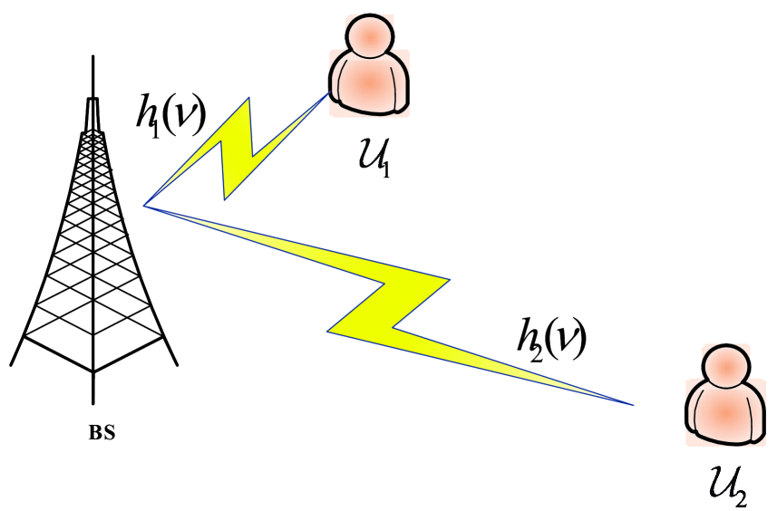
Figure 1: System model for a two-user downlink NOMA.

II-A Full CSIT

In this paper, we investigate two types of CSIT, i.e., full CSIT and partial CSIT, while CSI at the Rxs is assumed to be perfectly known. When full CSIT is available, the BS can adapt its power and rate of the transmit signal intended for each user to the channel $h_{k}(\nu)$’s in each fading state. On the other hand, when only partial CSIT including the order of the two channel gains and their channel distribution information (CDI) is available, due to some reasons like limited feedback from the users to the BS or reducing signalling for the purpose of reducing overhead, the BS can only determine its power allocation policy at each fading state based on this order. We also consider two different multiple access transmission schemes, viz., NOMA and optimal OMA. In the NOMA transmission scheme, the two users non-orthogonally access the channel by enabling superposition coding (SC) at the BS and SIC at the users. For optimal OMA transmission, we consider power and (continuous) time/frequency allocation both in an adaptive manner, which is referred as OMA-TYPE-II [15]. (Another benchmark scheme, OMA-Type-I, will be introduced in Section V.)

II-A1 NOMA

For NOMA transmission, the received signal at the downlink user $\mathcal{U}_{k}$ is given by

$$y_{k}(\nu)=\sqrt{p_{k}(\nu)}h_{k}(\nu)s_{k}+\sqrt{p_{\bar{k}}(\nu)}h_{k}(\nu)s_{\bar{k}}+n_{k},$$ (1)

where $\bar{k}$ denotes the element in the complementary set of $\{1,2\}$ w.r.t. $k$; $s_{k}$’s is the transmit signal intended for $\mathcal{U}_{k}$’s, denoted by $s_{k}\sim\mathcal{CN}(0,1)$; $p_{k}(\nu)$’s denotes $\mathcal{U}_{k}$’s transmit power; and $n_{k}$’s is the AWGN at $\mathcal{U}_{k}$’s Rx, denoted by $n_{k}\sim\mathcal{CN}(0,\sigma_{k}^{2})$.

We also define $\mathcal{U}_{k}$’s achievable rate for decoding $\mathcal{U}_{\bar{k}}$’s message at fading state $\nu$ in bits/sec/Hz, $k\in\{1,2\}$, treating interference as noise (TIAN), as follows.

$$R_{k\rightarrow\bar{k}}^{\rm NOMA}(\nu)=\log_{2}\left(1+\frac{p_{\bar{k}}(\nu)g_{k}(\nu)}{p_{k}(\nu)g_{k}(\nu)+1}\right),$$ (2)

where $g_{k}(\nu)$ is the normalized channel gain given by $\frac{|h_{k}(\nu)|^{2}}{\sigma_{k}^{2}}\triangleq g_{k}(\nu)$. Similarly, the achievable rate for $\mathcal{U}_{k}$ to decode its own message by TIAN is given by

$$R_{k\rightarrow k}^{\rm NOMA}(\nu)=\log_{2}\left(1+\frac{p_{k}(\nu)g_{k}(\nu)}{p_{\bar{k}}(\nu)g_{k}(\nu)+1}\right).$$ (3)

If $g_{k}(\nu)>g_{\bar{k}}(\nu)$, it implies that $R_{k\rightarrow\bar{k}}^{\rm NOMA}(\nu)>R_{\bar{k}\rightarrow\bar{k}}^{\rm NOMA}(\nu)$. In other words, under this condition, the achievable rate for $\mathcal{U}_{k}$ (the stronger user) to decode the message of $\mathcal{U}_{\bar{k}}$ (the weaker user) is larger than that intended for $\mathcal{U}_{\bar{k}}$’s transmission, and therefore $\mathcal{U}_{k}$ is able to successfully perform SIC. Otherwise, $\mathcal{U}_{k}$ is only able to decode its own message by TIAN. To sum up, the instantaneous achievable rate for $\mathcal{U}_{k}$’s is thus given by [18]

$$R_{k}^{\rm NOMA}(\nu)=$$

$$\left\{\begin{array}[]{l}\log_{2}\left(1+p_{k}(\nu)g_{k}(\nu)\right),\ {\rm if}\ g_{k}(\nu)>g_{\bar{k}}(\nu),\\ R_{k\rightarrow k}^{\rm NOMA}(\nu),\ {\rm otherwise.}\end{array}\right.$$ (6)

Moreover, similar to [21], we simultaneously consider two types of transmit power constraints on $p_{k}$’s, namely, average power constraint (APC) and peak power constraint (PPC), in which the former constrains the total transmit power in the long term, i.e., $\mathbb{E}_{\nu}[p_{k}(\nu)+p_{\bar{k}}(\nu)]\leq\bar{P}$, and the latter limits the instantaneous total transmit power below $\hat{P}$, i.e., $p_{k}(\nu)+p_{\bar{k}}(\nu)\leq\hat{P}$, $\forall\nu$. It is assumed that $\bar{P}\leq\hat{P}$ without loss of generality (w.l.o.g.).

II-A2 OMA-Type-II

For OMA-Type-II transmission, each user receives its information over $\alpha_{k}(\nu)$ of the time/frequency dedicated to it in fading state $\nu$, such that $\alpha_{k}(\nu)+\alpha_{\bar{k}}(\nu)=1$, where $\alpha_{k}(\nu)\in[0,1]$. The same sets of transmit power constraints as in its NOMA counterpart, i.e., APC and PPC, are taken into account as well. Accordingly, the instantaneous achievable rate for $\mathcal{U}_{k}$’s in fading state $\nu$ is given by

$$R_{k}^{\rm OMA\text{-}II}(\nu)=\alpha_{k}(\nu)\log_{2}\left(1+\frac{p_{k}(\nu)g_{k}(\nu)}{\alpha_{k}(\nu)}\right).$$ (7)

Note that (7) applies to both TDMA and FDMA transmission in the sense that the total energy consumed for the two users in fading state $\nu$ over time remains the same as that over frequency, which is given by $\alpha_{k}(\nu)\frac{p_{k}(\nu)}{\alpha_{k}(\nu)}+\alpha_{\bar{k}}(\nu)\frac{p_{\bar{k}}(\nu)}{\alpha_{\bar{k}}(\nu)}=p_{k}(\nu)+p_{\bar{k}}(\nu)$, $\forall\nu$.

II-B Partial CSIT

II-B1 NOMA

Under partial CSIT, for NOMA transmission, the BS does not know the exact CSI of the two users due to insufficient channel estimation but their relation, i.e., whether $g_{k}(\nu)\leq g_{\bar{k}}(\nu)$ or $g_{k}(\nu)<g_{\bar{k}}(\nu)$, and statistical characteristics, and therefore the Tx cannot dynamically adjust the allocation of power, rate and/or time/frequency resources to each fading state as in full CSIT. Hence, we adopt a binary power allocation strategy depending on which user has better CSI. Specifically, in each fading state $\nu$, an amount of power $p_{s}$ is always assigned to the stronger user while $p_{w}$ is assigned to the other weaker user. We also assume that $p_{s}$ and $p_{w}$ are static over all fading states, and therefore only APC applies, i.e., $p_{s}+p_{w}\leq\bar{P}$. In this case, the instantaneous rate $R_{k}^{\prime\rm NOMA}(\nu)$’s for $\mathcal{U}_{k}$’s is expressed as

$$R_{k}^{\prime\rm NOMA}(\nu)=$$

$$\left\{\begin{array}[]{l}\log_{2}\left(1+p_{s}g_{k}(\nu)\right),\ {\rm if}\ g_{k}(\nu)>g_{\bar{k}}(\nu),\\ \log_{2}\left(1+\frac{p_{w}g_{k}(\nu)}{p_{s}g_{k}(\nu)+1}\right),\ {\rm otherwise.}\end{array}\right.$$ (10)

II-B2 OMA-Type-II

Similarly, for OMA-Type-II transmission, the binary allocation policy with a fixed sharing of time/frequency between the two users is adopted. Specifically, the signal intended for $\mathcal{U}_{k}$ is transmitted with power $p_{s}$ if its channel gain from the BS is stronger than $\mathcal{U}_{\bar{k}}$’s, and with power $p_{w}$ otherwise. The fixed proportion of time/frequency assigned to $\mathcal{U}_{k}$ and $\mathcal{U}_{\bar{k}}$ is $\alpha_{k}$ and $\alpha_{\bar{k}}$, respectively. Consequently, the instantaneous achievable rate for $\mathcal{U}_{k}$’s is expressed as

$$R_{k}^{\prime\rm OMA\text{-}II}(\nu)=$$

$$\left\{\begin{array}[]{l}\alpha_{k}\log_{2}\left(1+\frac{p_{s}g_{k}(\nu)}{\alpha_{k}}\right),\ {\rm if}\ g_{k}(\nu)>g_{\bar{k}}(\nu),\\ \alpha_{k}\log_{2}\left(1+\frac{p_{w}g_{k}(\nu)}{\alpha_{k}}\right),\ {\rm otherwise.}\end{array}\right.$$ (13)

II-C System Throughput

II-C1 Delay-Tolerant Transmission

First, for “delay-tolerant” transmission, we refer it to the scenario in which no delay constraints are imposed for decoding, and thus the codeword can be designed arbitrarily long (approaching infinity in theory ) spanning over all the fading states, and decoded until it is received in its full length. The associated performance metric for each user is ergodic rate [18], at which the Tx delivers the intended data for each user over the entire fading process. Consequently, the ergodic sum-rate (ESR) of the two users are given by $\mathbb{E}_{\nu}[R_{k}^{\rm NOMA}(\nu)+R_{\bar{k}}^{\rm NOMA}(\nu)]$ ($\mathbb{E}_{\nu}[R_{k}^{\prime\rm NOMA}(\nu)+R_{\bar{k}}^{\prime\rm NOMA}(\nu)]$), and $\mathbb{E}_{\nu}[R_{k}^{\rm OMA\text{-}II}(\nu)+R_{\bar{k}}^{\rm OMA\text{-}II}(\nu)]$ ($\mathbb{E}_{\nu}[R_{k}^{\prime\rm OMA\text{-}II}(\nu)+R_{\bar{k}}^{\prime\rm OMA\text{-}II}(\nu)]$), for NOMA and OMA-Type-II transmission, respectively.

II-C2 Delay-Limited Transmission

Next, consider the delay-limited types of transmission for downlink NOMA and/or OMA-Type-II system. We relax the classical information theoretic “zero-outage” definition in [26]. Other than maintain a constant rate vector at all fading states via power control, we refer this notion to the scenario in which delay-sensitive data such as video streaming requires to be correctly decoded at a constant rate at the end of every fading state. The associated performance metric for each user is outage probability, which measures the percentage of fading states at which a predefined constant rate cannot be supported.

Specifically, under full CSIT, the outage probability for user $\mathcal{U}_{k}$ with the target rate $\bar{R}_{k}$, $k\in\{1,2\}$, is introduced as below.
Case 1: $g_{k}(\nu)>g_{\bar{k}}(\nu)$

$$\zeta_{k}^{\rm NOMA}=\Pr\left\{R_{k\rightarrow\bar{k}}^{\rm NOMA}(\nu)<\bar{R}_{\bar{k}},R_{k\rightarrow k}^{\rm NOMA}(\nu)<\bar{R}_{k}\right\}+\\ \Pr\left\{R_{k\rightarrow\bar{k}}^{\rm NOMA}(\nu)\geq\bar{R}_{\bar{k}},R_{k}^{\rm NOMA}(\nu)<\bar{R}_{k}\right\}.$$ (14)

Case 2: $g_{k}(\nu)\leq g_{\bar{k}}(\nu)$

$$\zeta_{k}^{\rm NOMA}=\Pr\left\{R_{k}^{\rm NOMA}(\nu)<\bar{R}_{k}\right\}.$$ (15)

As seen from (14), when $\mathcal{U}_{k}$ has better channel condition, whether its signal-to-noise ratio (SNR) or signal-to-interference-plus-noise ratio (SINR) leads to its outage depends on whether or not it manages to recover $\mathcal{U}_{\bar{k}}$’s message. If it fails to retrieve $\mathcal{U}_{\bar{k}}$’s message at the predefined transmission rate for $\mathcal{U}_{\bar{k}}$, i.e., $\bar{R}_{\bar{k}}$, it has to decode its own by TIAN. Otherwise, if it succeeds in decoding $\mathcal{U}_{\bar{k}}$’s message, SIC is performed before it decodes its own interference-free. On the other hand, when $\mathcal{U}_{k}$ has worse channel condition, it always decodes its own by TIAN (c.f. (15)).

In addition, at each fading state $\nu$, an outage indicator function is defined as follows [20].
Case 1: $g_{k}(\nu)>g_{\bar{k}}(\nu)$

$$X_{k}^{\rm NOMA}(\nu)=$$

$$\left\{\begin{array}[]{ll}1,&{\rm if}\ R_{k\rightarrow\bar{k}}^{\rm NOMA}(\nu)<\bar{R}_{\bar{k}},\ R_{k\rightarrow k}^{\rm NOMA}(\nu)<\bar{R}_{k},\\ 1,&{\rm if}\ R_{k\rightarrow\bar{k}}^{\rm NOMA}(\nu)\geq\bar{R}_{\bar{k}},\ R_{k}^{\rm NOMA}(\nu)<\bar{R}_{k},\\ 0,&{\rm otherwise.}\end{array}\right.$$ (19)

Case 2: $g_{k}(\nu)\leq g_{\bar{k}}(\nu)$

$$X_{k}^{\rm NOMA}(\nu)=\left\{\begin{array}[]{ll}1,&{\rm if}\ \ R_{k\rightarrow k}^{\rm NOMA}(\nu)<\bar{R}_{k},\\ 0,&{\rm otherwise.}\end{array}\right.$$ (22)

Combining (19) (c.f. (14)) and (22) (c.f. (15)), it is easily verified that $\mathbb{E}_{\nu}[X_{k}^{\rm NOMA}(\nu)]=\zeta_{k}^{\rm NOMA}$, $k\in\{1,2\}$.

For OMA-Type-II transmission, the outage probability of $\mathcal{U}_{k}$’s is defined independent of the other as follows:

$$\zeta_{k}^{\rm OMA\text{-}II}=\Pr\left\{R_{k}^{\rm OMA\text{-}II}(\nu)<\bar{R}_{k}\right\}.$$ (23)

By analogy, we introduce the following indicator function for $\mathcal{U}_{k}$ w.r.t. the target rate $\bar{R}_{k}$:

$$X_{k}^{\rm OMA\text{-}II}(\nu)=\left\{\begin{array}[]{ll}1,&{\rm if}\ R_{k}^{\rm OMA\text{-}II}(\nu)<\bar{R}_{k},\\ 0,&{\rm otherwise.}\end{array}\right.$$ (26)

It also follows that $\mathbb{E}_{\nu}[X_{k}^{\rm OMA\text{-}II}(\nu)]=\zeta_{k}^{\rm OMA\text{-}II}$, $k\in\{1,2\}$.

Accordingly, one relevant metric to assess the overall performance in delay-limited case is the sum of DLT expressed as $\bar{R}_{k}(1-\zeta_{k}^{\rm NOMA})+\bar{R}_{\bar{k}}(1-\zeta_{\bar{k}}^{\rm NOMA})$, and $\bar{R}_{k}(1-\zeta_{k}^{\rm OMA\text{-}II})+\bar{R}_{\bar{k}}(1-\zeta_{\bar{k}}^{\rm OMA\text{-}II})$, for NOMA and OMA-Type-II transmission under full CSIT, respectively. The sum of DLT for NOMA and OMA-Type-II transmission under partial CSIT is also similarly given by $\bar{R}_{k}(1-\zeta_{k}^{\prime\rm NOMA})+\bar{R}_{\bar{k}}(1-\zeta_{\bar{k}}^{\prime\rm NOMA})$, and $\bar{R}_{k}(1-\zeta_{k}^{\prime\rm OMA\text{-}II})+\bar{R}_{\bar{k}}(1-\zeta_{\bar{k}}^{\prime\rm OMA\text{-}II})$, respectively.

III Optimum Delay-Tolerant Transmission

In delay-tolerant scenarios, to maximize the ESR of the system while guaranteeing certain level of fairness, a minimum achievable ergodic rate requirement for each user, namely, $\mathbb{E}_{\nu}[R_{k}^{\rm XX}(\nu)]\geq\bar{R}$ ($\mathbb{E}_{\nu}[R_{k}^{\prime\rm XX}(\nu)]\geq\bar{R}^{\prime}$), $k\in\{1,2\}$, is imposed, where $(\cdot)^{\rm XX}$ denotes the multiple access scheme that is specified in the context throughout the paper. In this section, the optimal trade-off between the system ESR and user fairness is pursued in the case of full and partial CSIT, respectively. Particularly, under full CSIT, the ESR maximization problems are solved using Lagrangian dual decomposition levering “time-sharing” conditions, while under partial CSIT, individual user’s ergodic rate needs to be first analysed in closed form by means of CDFs of the related SNR and/or SNRs.

III-A Full CSIT

In the case of full CSIT, the design objective is to maximize the system ESR by jointly optimizing the power and/or orthogonal resource allocations, and the two users’ instantaneous rate at each fading state, subject to both APC and PPC at the BS, as well as a minimum ergodic rate constraint for the two users. As a result, the optimization problem is formulated as follows.

$$\mathrm{(P1\text{-}XX)}: ~{}~{}\mathop{\mathtt{Maximize}}_{\{p_{k}(\nu),p_{\bar{k}}(\nu),\alpha_{k}(\nu)\}}\mathbb{E}_{\nu}[R_{k}^{\rm XX}(\nu)+R_{\bar{k}}^{\rm XX}(\nu)]$$

$$~{}~{}\mathtt{Subject\ to}$$

$$~{}~{}\mathbb{E}_{\nu}[p_{k}(\nu)+p_{\bar{k}}(\nu)]\leq\bar{P},$$ (27a)

$$~{}~{}p_{k}(\nu)+p_{\bar{k}}(\nu)\leq\hat{P},\ \forall\nu,$$ (27b)

$$~{}~{}p_{k}(\nu)\geq 0,\ p_{\bar{k}}(\nu)\geq 0,\ \forall\nu,$$ (27c)

$$~{}~{}\mathbb{E}_{\nu}[R_{k}^{\rm XX}(\nu)]\geq\bar{R},\;\forall k,$$ (27d)

where the exclusive parameters for OMA-Type-II, $\{\alpha_{k}(\nu)\}$’s, are only valid when ${\rm XX}$ refers to OMA-Type-II. In the following, we develop optimal solution to $\mathrm{(P1\text{-}NOMA)}$ and $\mathrm{(P1\text{-}OMA\text{-}II)}$, respectively.

III-A1 Optimal Solution to $\mathrm{(P1\text{-}NOMA)}$

Problem $\mathrm{(P1\text{-}NOMA)}$ is non-convex due to the non-convex objective function (c.f. (6)), and therefore no immediate solution can be given. However, for channel fading following continuous distributions, $\mathrm{(P1\text{-}NOMA)}$ proves to satisfy the “time-sharing” condition. Note that if (P1-NOMA) satisfies the “time-sharing condition”, then it has a zero duality gap between the primal and the dual problem using Lagrangian duality [28, Theorem 1], i.e., strong duality [29] holds, despite of the convexity of the problem itself. Hence, we can still optimally solve it via its dual problem.

Next, we apply the Lagrangian dual method to solve $\mathrm{(P1\text{-}NOMA)}$, the Lagrangian of which is given by

$$\mathcal{L}_{1}^{\rm NOMA}(\{p_{k}(\nu)\},\{p_{\bar{k}}(\nu)\},\lambda,\delta,\mu)=\\ \mathbb{E}_{\nu}[(1+\delta)R_{k}^{\rm NOMA}(\nu)+(1+\mu)R_{\bar{k}}^{\rm NOMA}(\nu)-\lambda(p_{k}(\nu)+p_{\bar{k}}(\nu))]\\ +\lambda\bar{P}-\delta\bar{R}-\mu\bar{R},$$ (28)

where $\lambda$ is the Lagrangian multiplier associated with the APC given in (27a); $\delta$ and $\mu$ are those associated with the ergodic rate constraints given in (27d) for $\mathcal{U}_{k}$ and $\mathcal{U}_{\bar{k}}$, respectively. The dual function of $\mathrm{(P1\text{-}NOMA)}$ corresponding to (28) is accordingly given by

$$g(\lambda,\delta,\mu)=\max\mathcal{L}_{1}^{\rm NOMA}(\{p_{k}(\nu)\},\{p_{\bar{k}}(\nu)\},\lambda,\delta,\mu),$$

$$\mathtt{s.t.}~{}~{}p_{k}(\nu)\geq 0,p_{\bar{k}}(\nu)\geq 0,p_{k}(\nu)+p_{\bar{k}}(\nu)\leq\hat{P},\;\forall\nu.$$ (29)

The dual problem of $\mathrm{(P1\text{-}NOMA)}$ is thus formulated as

$$\mathrm{(P1\text{-}NOMA\text{-}dual)}:~{}\mathop{\mathtt{Minimize}}_{\lambda\geq 0,\delta\geq 0,\mu\geq 0} ~{}~{}~{}g(\lambda,\delta,\mu).$$

It is observed that $g(\lambda,\delta,\mu)$ is obtained by maximizing the Lagrangian given in (28), which can be decoupled into as many subproblems as the number of fading states all sharing the same structure. The index $\nu$ is now safely dropped for the ease of exposition. Taking one particular fading state as an example, the associated subproblem given a triple $(\lambda,\delta,\mu)$ can be expressed as

$$\mathrm{(P1\text{-}NOMA\text{-}sub)}:~{}\mathop{\mathtt{Maximize}}_{p_{k}\geq 0,p_{\bar{k}}\geq 0} ~{}~{}~{}\bar{\mathcal{L}}_{1}^{\rm NOMA}(p_{k},p_{\bar{k}})$$

$$\mathtt{Subject\ to} ~{}~{}~{}p_{k}+p_{\bar{k}}\leq\hat{P},$$

where $\bar{\mathcal{L}_{1}}^{\rm NOMA}(p_{k},p_{\bar{k}})=(1+\delta)R_{k}^{\rm NOMA}+(1+\mu)R_{\bar{k}}^{\rm NOMA}-\lambda(p_{k}+p_{\bar{k}})$. Since these problems are independent of each other, they can be solved in parallel each for one fading state. Therefore, w.l.o.g., we focus on solving $\mathrm{(P1\text{-}NOMA\text{-}sub)}$ in the sequel.

Proposition III.1

The optimal power allocation to Problem $\mathrm{(P1\text{-}NOMA\text{-}sub)}$ assuming $g_{1}>g_{2}$ is given by

$$(p_{1}^{\ast},p_{2}^{\ast})=\arg\max\{\bar{\mathcal{L}}_{1}^{\rm NOMA}(0,0),\bar{\mathcal{L}}_{1}^{\rm NOMA}(0,\hat{P}),\\ \bar{\mathcal{L}}_{1}^{\rm NOMA}(\hat{P},0),\bar{\mathcal{L}}_{1}^{\rm NOMA}(p_{i,1},p_{i,2})\},\;i\in\{1,2,3,4\},$$ (30)

where $(p_{i,1},p_{i,2})$, $i\in\{1,2,3,4\}$, are given at the top of the next page with each corresponding to one solution pair given by (40).

Proof:

Since $\bar{\mathcal{L}}_{1}^{\rm NOMA}(p_{1},p_{2})$ is a continuous function over $\Psi=\{(p_{1},p_{2})|p_{1}\geq 0,p_{2}\geq 0,p_{1}+p_{2}\leq\hat{P}\}$, its maximum proves to be either at the stationary point, denoted by $(p_{4,1},p_{4,2})$, or on the boundary of $\Psi$ depending on whether $(p_{4,1},p_{4,2})\in\Psi$ or not. We calculate $(p_{4,1},p_{4,2})$ as follows:

$$(p_{4,1},p_{4,2})=\arg\left\{\nabla_{(p_{1},p_{2})}\bar{\mathcal{L}}_{1}^{\rm NOMA}(p_{1},p_{2})=\mbox{\boldmath{$0$}}\right\}.$$ (31)

If $(p_{4,1},p_{4,2})\in\Psi$, the maximum is $\bar{\mathcal{L}}_{1}^{\rm NOMA}(p_{4,1},p_{4,2})$, otherwise the maximum can be attained by restricting $(p_{1},p_{2})$ to the lines $p_{1}=0$, $p_{2}=0$ or $p_{1}+p_{2}=\hat{P}$. The stationary points on these lines are denoted by $(p_{i,1},p_{i,2})$’s, $i=1$, $2$ and $3$, respectively. ∎

Note that Proposition III.1 assumes $g_{1}>g_{2}$ for the ease of exposition though, its results also apply to the fading states where $g_{1}<g_{2}$ by simply exchanging $\delta$, $p_{1}$, and $g_{1}$ with $\mu$, $p_{2}$, and $g_{2}$, respectively, in (40). Some optimal system design insights are gained from Proposition III.1. Considering an extreme case in favour of $\mathcal{U}_{2}$, in which $\delta\ll\mu$, it is observed from (40) that $p_{4,1}$ monotonically decreases with $\mu$ while $p_{4,2}$ monotonically increases with $\mu$, which suggests that when $\mu$ associated with $\mathcal{U}_{2}$’s QoS requirement is sufficiently large, the optimal power allocation policy tends to suppress $\mathcal{U}_{1}$’s transmission while supporting $\mathcal{U}_{2}$’s despite of $\mathcal{U}_{1}$’s channel condition better than $\mathcal{U}_{2}$.

$$\kern-8.0pt\left\{\begin{array}[]{ll}p_{1,1}=0,&p_{1,2}=\left[\frac{1+\mu}{\lambda\ln 2}-\frac{1}{g_{2}}\right]_{0}^{\hat{P}}\\ p_{2,1}=\left[\frac{1+\delta}{\lambda\ln 2}-\frac{1}{g_{1}}\right]_{0}^{\hat{P}},&p_{2,2}=0\\ p_{3,1}=\left[\frac{(1+\mu)\mathord{\left/\right.\kern-1.2pt}g_{1}-(1+\delta)\mathord{\left/\right.\kern-1.2pt}g_{2}}{\delta-\mu}\right]_{0}^{\hat{P}},&p_{3,2}=\left[\hat{P}-\frac{(1+\mu)\mathord{\left/\right.\kern-1.2pt}g_{1}-(1+\delta)\mathord{\left/\right.\kern-1.2pt}g_{2}}{\delta-\mu}\right]_{0}^{\hat{P}}\\ \left\{\begin{array}[]{l}p_{4,1}=\frac{(1+\mu)\mathord{\left/\right.\kern-1.2pt}g_{1}-(1+\delta)\mathord{\left/\right.\kern-1.2pt}g_{2}}{\delta-\mu}\\ p_{4,2}=\frac{1+\mu}{\lambda\ln 2}-\frac{1}{g_{2}}-\frac{(1+\mu)\mathord{\left/\right.\kern-1.2pt}g_{1}-(1+\delta)\mathord{\left/\right.\kern-1.2pt}g_{2}}{\delta-\mu}\end{array},\right.&\left.\begin{array}[]{l}\mbox{if}\ p_{4,1}\geq 0,p_{4,2}\geq 0,p_{4,1}+p_{4,2}\leq\hat{P},\\ \mbox{N/A, otherwise.}\end{array}\right.\end{array}\right.$$ (40)

Thanks to Proposition III.1, given a triple $(\lambda,\delta,\mu)$, $g(\lambda,\delta,\mu)$ is obtained efficiently by solving $\mathrm{(P1\text{-}NOMA\text{-}sub)}$ in parallel over all fading states. $\mathrm{(P1\text{-}NOMA\text{-}dual)}$ can thus be iteratively solved using sub-gradient based methods, e.g., deep-cut ellipsoid method (with constraints) [30, Localization methods]. The required sub-gradient for updating $(\lambda,\delta,\mu)$ turns out to be $(\bar{P}-\mathbb{E}_{\nu}[p_{k}^{\ast}(\nu)+p_{\bar{k}}^{\ast}(\nu)],\mathbb{E}_{\nu}[R_{k}^{\ast\rm NOMA}(\nu)]-\bar{R},\mathbb{E}_{\nu}[R_{\bar{k}}^{\ast\rm NOMA}(\nu)]-\bar{R})^{T}$, where $(p_{k}^{\ast}(\nu),p_{\bar{k}}^{\ast}(\nu))$ is the optimal solution to $\mathrm{(P1\text{-}NOMA\text{-}sub)}$ at fading state $\nu$, and $R_{k}^{\ast\rm NOMA}(\nu)$’s is obtained by substituting $(p_{k}^{\ast}(\nu),p_{\bar{k}}^{\ast}(\nu))$ into (6).

Note that a feasible $\bar{R}$ in (27d) ensures the successful implementation of the ellipsoid method, and thus it is important to consider a reasonable $\bar{R}$ that does not exceed $\bar{R}_{\max}$. We can obtain $\bar{R}_{\max}$ by replacing the objective function of $\mathrm{(P1\text{-}NOMA)}$ with a variable $\bar{R}$ and then solving the feasibility problem by bi-section over $\bar{R}$. Since the involved procedure is quite similar to that for solving $\mathrm{(P1\text{-}NOMA)}$, we omit it herein for brevity.

III-A2 Optimal Solution to $\mathrm{(P1\text{-}OMA\text{-}II)}$

First, $\mathrm{(P1\text{-}OMA\text{-}II)}$ is a convex problem, since (7) as the perspective of the jointly concave function $\log_{2}(1+p_{k}(\nu)g_{k}(\nu))$ proves to be jointly concave w.r.t. $\alpha_{k}(\nu)$ and $p_{k}(\nu)$, $k\in\{1,2\}$, $\forall\nu$. As such, we can solicit the Lagrangian dual method to solve $\mathrm{(P1\text{-}OMA\text{-}II)}$ due to strong duality.

The Lagrangian of $\mathrm{(P1\text{-}OMA\text{-}II)}$ is expressed as

$$\mathcal{L}_{1}^{\rm OMA\text{-}II}(\{p_{k}(\nu)\},\{p_{\bar{k}}(\nu)\},\{\alpha_{k}(\nu)\},\lambda,\delta,\mu)=\\ \mathbb{E}_{\nu}[(1+\delta)R_{k}^{\rm OMA\text{-}II}(\nu)+(1+\mu)R_{\bar{k}}^{\rm OMA\text{-}II}(\nu)-\lambda(p_{k}(\nu)+p_{\bar{k}}(\nu))]\\ +\lambda\bar{P}-\delta\bar{R}-\mu\bar{R},$$ (41)

where $\lambda$, $\delta$ and $\mu$ are Lagrangian multipliers associated with the same constraints as those for $\mathrm{(P1\text{-}NOMA)}$. Similar to the previous section, $\mathcal{L}_{1}^{\rm OMA\text{-}II}(\{p_{k}(\nu)\},\{p_{\bar{k}}(\nu)\},\{\alpha_{k}(\nu)\},\lambda,\delta,\mu)$ can also be decoupled into parallel sub-Lagrangian all having the same structure. We define $\bar{\mathcal{L}}_{1}^{\rm OMA\text{-}II}(p_{k},p_{\bar{k}},\alpha_{k})=(1+\delta)R_{k}^{\rm OMA\text{-}II}+(1+\mu)R_{\bar{k}}^{\rm OMA\text{-}II}-\lambda(p_{k}+p_{\bar{k}})$. Then the associated subproblem one particular fading state is formulated as

$$\mathrm{(P1\text{-}OMA\text{-}II\text{-}sub)}:~{}\mathop{\mathtt{Maximize}}_{p_{k}\geq 0,p_{\bar{k}}\geq 0,\alpha_{k}} ~{}~{}~{}\bar{\mathcal{L}}_{1}^{\rm OMA\text{-}II}(p_{k},p_{\bar{k}},\alpha_{k})$$

$$\mathtt{Subject\ to} ~{}~{}~{}p_{k}+p_{\bar{k}}\leq\hat{P},$$

$$~{}~{}~{}0\leq\alpha_{k}\leq 1,\;\forall k,$$

where the index $\nu$ has been dropped for the ease of exposition. To solve $\mathrm{(P1\text{-}OMA\text{-}II\text{-}sub)}$, the following two lemmas are required.

Lemma III.1

If the maximum of $\bar{\mathcal{L}}_{1}^{\rm OMA\text{-}II}(p_{1},p_{2},\alpha_{1})$ is achieved by its jointly stationary point, it is necessary to have the following conditions satisfied:

$$h(\lambda,\delta,\mu)=0,$$ (42a)

$$c_{1}\geq 0,$$ (42b)

$$c_{2}\geq 0,$$ (42c)

$$\left\{\begin{array}[]{ll}\frac{\hat{P}-c_{2}}{c_{1}-c_{2}}\geq 0,&{\rm if}\ c_{1}>c_{2},\\ \frac{\hat{P}-c_{2}}{c_{1}-c_{2}}\leq 1,&{\rm otherwise,}\end{array},\right.$$ (42f)

where $c_{1}=\frac{1+\delta}{\lambda\ln 2}-\frac{1}{g_{1}}$, $c_{2}=\frac{1+\mu}{\lambda\ln 2}-\frac{1}{g_{2}}$, and $h(\lambda,\delta,\mu)$ is given by

$$h(\lambda,\delta,\mu)=(1+\delta)\log_{2}\left(\frac{1+\delta}{\lambda\ln 2}g_{1}\right)-\\ (1+\mu)\log_{2}\left(\frac{1+\mu}{\lambda\ln 2}g_{2}\right)-\lambda c_{1}+\lambda c_{2}.$$ (43)

The corresponding stationary point is given by

$$p_{1}^{\ast}=c_{1}\alpha_{1}^{\ast},\ p_{2}^{\ast}=c_{2}(1-\alpha_{1}^{\ast}),$$ (44)

where

$$\alpha_{1}^{\ast}=\left\{\begin{array}[]{ll}\forall\in[0,\min\{\frac{\hat{P}-c_{2}}{c_{1}-c_{2}},1\}],&{\rm if}\ c_{1}>c_{2},\\ \forall\in[(\frac{\hat{P}-c_{2}}{c_{1}-c_{2}})^{+},1],&{\rm otherwise.}\end{array}\right.$$ (47)

Proof:

First, solve $\nabla_{(p_{1},p_{2},\alpha_{1})}\bar{\mathcal{L}}_{1}^{\rm OMA\text{-}II}(p_{1},p_{2},\alpha_{1})=\mbox{\boldmath{$0$}}$ to obtain the jointly stationary point. Next, by plugging $p_{1}=c_{1}\alpha_{1}$ and $p_{2}=c_{2}(1-\alpha_{1})$ into the partial derivative of $\bar{\mathcal{L}}_{1}^{\rm OMA\text{-}II}(p_{1},p_{2},\alpha_{1})$ w.r.t. $\alpha_{1}$, (42a) is obtained. Finally, constrain $P_{1}\geq 0$, $p_{2}\geq 0$, and $p_{1}+p_{2}\leq\hat{P}$, we arrive at (42b), (42c), and the feasible range for $\alpha_{1}$ given in (47), respectively. ∎

Lemma III.2

If the maximum of $\bar{\mathcal{L}}_{1}^{\rm OMA\text{-}II}(p_{1},p_{2},\alpha_{1})$ is achieved by points on the boundary $p_{1}+p_{2}=\hat{P}$, the optimum $(p_{1},p_{2},\alpha_{1})$ turns out to be

$$\left\{\begin{array}[]{ll}p_{1}^{\ast}=0,\ p_{2}^{\ast}=\hat{P},\ \alpha_{1}^{\ast}=0,&{\rm if}\ \frac{1+\mu}{1+\delta}>\frac{\log_{2}(1+\hat{P}g_{1})}{\log_{2}(1+\hat{P}g_{2})},\\ p_{1}^{\ast}=\hat{P},\ p_{2}^{\ast}=0,\ \alpha_{1}^{\ast}=1,&{\rm otherwise.}\end{array}\right.$$ (50)

Proof:

Please refer to Appendix A. ∎

Based on Lemma III.1 and Lemma III.2, the following proposition is derived.

Proposition III.2

The optimal power as well as time/frequency allocation to $\mathrm{(P1\text{-}OMA\text{-}II\text{-}sub)}$ is given by

$$(p_{1}^{\ast},p_{2}^{\ast},\alpha_{1}^{\ast})=\arg\max\{\bar{\mathcal{L}}_{1}^{\rm OMA\text{-}II}(0,0,0),\\ \bar{\mathcal{L}}_{1}^{\rm OMA\text{-}II}(0,\hat{P},0),\bar{\mathcal{L}}_{1}^{\rm OMA\text{-}II}(\hat{P},0,1),\\ \bar{\mathcal{L}}_{1}^{\rm OMA\text{-}II}(0,c_{2},0)\mathbbm{1}_{c_{2}},\bar{\mathcal{L}}_{1}^{\rm OMA\text{-}II}(c_{1},0,1)\mathbbm{1}_{c_{1}}\},$$ (51)

where $\mathbbm{1}_{(\cdot)}$ is an indicator function defined as

$$\mathbbm{1}_{x}=\left\{\begin{array}[]{ll}1,&{\rm if}\ 0\leq x\leq\hat{P},\\ 0,&{\rm otherwise.}\end{array}\right.$$ (54)

Proof:

Please refer to Appendix B. ∎

Remark III.1

When there are only two users, the optimal solution given by (51) shares some philosophy in common with that achieves the boundary of the time division (TD) capacity region discussed in [18, Theorem 3]. We focus on solving $\mathrm{(P1\text{-}OMA\text{-}II\text{-}sub)}$ in any fading state given a triple $(\lambda,\delta,\mu)$, while [18] maximized the total weighted sum-rate in any fading state by determining how to distribute $P(\mbox{\boldmath{$n$}})$ among $M=2$ users such that the instantaneous total power constraint $\sum_{j=1}^{2}\tau_{j}P_{j}(\mbox{\boldmath{$n$}})=P(\mbox{\boldmath{$n$}})$ (c.f. [18, Eqn. (11)]) is satisfied. The optimal solutions both suggest that with probability $1$, at most one single user transmits in any fading state. This is because the probability measure of any subset of $\{(g_{k}(\nu),g_{\bar{k}}(\nu)):h(\lambda,\delta,\mu)=0\}$ (c.f. (43)) assuming continuously joint distribution of $(g_{k}(\nu),g_{\bar{k}}(\nu))$ is zero, as is the probability measure of $\{\mbox{\boldmath{$n$}}:h(\lambda,\mbox{\boldmath{$n$}})=0\}$ in [18, Theorem 3]. This also explains why the maximum of $\bar{\mathcal{L}}_{1}^{\rm OMA\text{-}II}(p_{1},p_{2},\alpha_{1})$ cannot be achieved by its jointly stationary point in probability.

With Proposition III.2, given a triple $(\lambda,\delta,\mu)$, $\mathrm{(P1\text{-}OMA\text{-}II\text{-}sub)}$ is first solved state by state; then by updating $(\lambda,\delta,\mu)$ in accordance with the associated sub-gradient $(\bar{P}-\mathbb{E}_{\nu}[p_{k}(\nu)+p_{\bar{k}}(\nu)],\mathbb{E}_{\nu}[R_{k}^{\rm OMA\text{-}II}(\nu)]-\bar{R},\mathbb{E}_{\nu}[R_{\bar{k}}^{\rm OMA\text{-}II}(\nu)]-\bar{R})^{T}$, $\mathrm{(P1\text{-}OMA\text{-}II)}$ is iteratively solved.

Next, we rigorously prove that the ESR achieved by OMA-Type-II cannot perform better than that achieved by NOMA. To prove so, we denote the optimal power and time/frequency allocation to $\mathrm{(P1\text{-}OMA\text{-}II)}$ by $\{p_{1}^{\ast}(\nu),p_{2}^{\ast}(\nu),\alpha_{1}^{\ast}(\nu)\}$. Then let $p_{1}=p_{1}^{\ast}$ and $p_{2}=p_{2}^{\ast}$ in each fading state for NOMA transmission. If an alternative user is selected to transmit, then the optimum $\alpha_{k}$ associated with it is seen to be $1$ (c.f. (51)). Hence, assuming $p_{1}^{\ast}>0$ ($\alpha_{1}^{\ast}=1$) and $p_{2}^{\ast}=0$ ($\alpha_{2}^{\ast}=0$), $R_{1}^{\rm NOMA}$ turns out be $\log_{2}(1+p_{1}^{\ast}g_{1})$ and $R_{2}^{\rm NOMA}=0$, which is exactly equal to $R_{1}^{\ast\rm OMA\text{-}II}$ and $R_{2}^{\ast\rm OMA\text{-}II}$, respectively; vice versa when $p_{1}^{\ast}=0$ ($\alpha_{1}^{\ast}=0$) and $p_{2}^{\ast}>0$ ($\alpha_{2}^{\ast}=1$). The other trivial case is that $R_{k}^{\rm NOMA}=R_{k}^{\ast\rm OMA\text{-}II}=0$, $\forall k$, when $p_{1}^{\ast}=p_{2}^{\ast}=0$. Hence, with $p_{1}=p_{1}^{\ast}$ and $p_{2}=p_{2}^{\ast}$ in each fading state, $\mathbb{E}_{\nu}[R_{k}^{\rm NOMA}(\nu)]=\mathbb{E}_{\nu}[R_{k}^{\ast\rm OMA\text{-}II}(\nu)]\geq\bar{R}$, $\forall k$, is met. It is also easily examined that (27d) is satisfied. To sum up, the optimal solution to $\mathrm{(P1\text{-}OMA\text{-}II)}$ proves to be feasible to $\mathrm{(P1\text{-}NOMA)}$, the former of which thus yields an optimum value no more than the latter.

III-B Partial CSIT

By analogy, the partial CSIT counterpart of Problem $\mathrm{(P1\text{-}XX)}$ is formulated as below:

$$\mathrm{(P1^{\prime}\text{-}XX)}:~{}\mathop{\mathtt{Maximize}}_{p_{s},p_{w},\alpha_{k}} ~{}~{}~{}\mathbb{E}_{\nu}[R_{k}^{\prime\rm XX}(\nu)+R_{\bar{k}}^{\prime\rm XX}(\nu)]$$

$$\mathtt{Subject\ to} ~{}~{}~{}p_{s}+p_{w}\leq\bar{P},$$ (55a)

$$~{}~{}~{}p_{s}\geq 0,\ p_{w}\geq 0,$$ (55b)

$$~{}~{}~{}\mathbb{E}_{\nu}[R_{k}^{\prime\rm XX}(\nu)]\geq\bar{R}^{\prime},\;\forall k,$$ (55c)

where $\alpha_{k}$’s is only valid in the transmission adopting OMA-Type-II. Similar to Problem $\mathrm{(P1\text{-}XX)}$, (55c) constrain the minimum average user rate achieved by the two users. In the following, we provide optimal solution to $\mathrm{(P1^{\prime}\text{-}NOMA)}$ and $\mathrm{(P1^{\prime}\text{-}OMA\text{-}II)}$, respectively.

III-B1 Optimal Solution to $\mathrm{(P1^{\prime}\text{-}NOMA)}$

Since only the relation between the two users’ channel gains at each fading state and their CDI are known to the BS, we first derive the expectation of $R_{k}^{\prime\rm NOMA}(\nu)$’s as function of $p_{s}$ and $p_{w}$, and then solve $\mathrm{(P1^{\prime}\text{-}NOMA)}$ in accordance with these expectation results.

First, denote the RV $|h_{k}(\nu)|^{2}$ ($|h_{\bar{k}}(\nu)|^{2}$) by $X$ ($Y$). Also, denote the SNR $p_{s}g_{k}(\nu)$ and the SINR $p_{w}g_{k}(\nu)\mathord{\left/\right.\kern-1.2pt}(p_{s}g_{k}(\nu)+1)$ (c.f. (10)) by $\Gamma_{k}$ and $\tilde{\Gamma}_{k}$, respectively. It thus follows that the conditional cumulative density functions (CDFs) of $\Gamma_{k}$ and $\tilde{\Gamma}_{k}$ are given by

$${F_{{\Gamma_{k|X\geq Y}}}}\left({{z}}\right)= \frac{\Pr\{p_{s}X\mathord{\left/\right.\kern-1.2pt}\sigma_{k}^{2}\leq z,X\geq Y\}}{\Pr\{X\geq Y\}}$$

$$= 1-\frac{\lambda_{k}+\lambda_{\bar{k}}}{\lambda_{\bar{k}}}{e^{-{\lambda_{k}}{\varepsilon_{k}}}}+\frac{\lambda_{k}}{\lambda_{\bar{k}}}e^{-\left(\lambda_{k}+\lambda_{\bar{k}}\right)\varepsilon_{k}},$$ (56)

$${F_{{\tilde{\Gamma}_{k}|X<Y}}}\left({{z}}\right)= \frac{\Pr\{p_{w}X\mathord{\left/\right.\kern-1.2pt}\left(p_{s}X+\sigma_{k}^{2}\right)\leq z,X<Y\}}{\Pr\{X<Y\}}$$

$$= \left\{\begin{array}[]{l}1,\ \ \mbox{if}\ {p_{w}}-{p_{s}}{z}\leq 0,\\ 1-{e^{-\left({{\lambda_{k}}+{\lambda_{\bar{k}}}}\right){\tilde{\varepsilon}_{k}}}},\ \ \mbox{otherwise,}\end{array},\right.$$ (59)

respectively, where $\varepsilon_{k}\triangleq\frac{\sigma_{k}^{2}z}{p_{s}}$ and $\tilde{\varepsilon}_{k}\triangleq\frac{\sigma_{k}^{2}z}{p_{w}-p_{s}z}$. In accordance with (56) and (59), $\mathbb{E}_{\nu}[R_{k}^{\prime\rm NOMA}(\nu)]$’s can be obtained by the following proposition.

Proposition III.3

The ergodic rate for NOMA user $\mathcal{U}_{k}$, $k\in\{1,2\}$, under partial CSIT is given by

$$\mathbb{E}_{\nu}[R_{k}^{\prime\rm NOMA}(\nu)]=\frac{2}{{\ln 2}}\frac{{{\lambda_{k}}}}{{{\lambda_{k}}+{\lambda_{\bar{k}}}}}f\left(\frac{{\left({{\lambda_{k}}+{\lambda_{\bar{k}}}}\right)\sigma_{k}^{2}}}{{{p_{s}}}}\right)\\ -\frac{1}{{\ln 2}}\frac{{{\lambda_{k}}}}{{{\lambda_{k}}+{\lambda_{\bar{k}}}}}f\left(\frac{{\left({{\lambda_{k}}+{\lambda_{\bar{k}}}}\right)\sigma_{k}^{2}}}{{{p_{s}+p_{w}}}}\right)-\frac{1}{{\ln 2}}f\left(\frac{{{\lambda_{k}}\sigma_{k}^{2}}}{{{p_{s}}}}\right),$$ (60)

where $f(\cdot)$ denotes the function $f(x)=e^{x}{\rm Ei}(-x)$ ($x>0$).

Proof:

Please refer to Appendix C. ∎

Since the optimization variable $p_{w}$ only contributes to $f(\frac{{\left({{\lambda_{k}}+{\lambda_{\bar{k}}}}\right)\sigma_{k}^{2}}}{{{p_{s}}+{p_{w}}}})$, we examine the property of $\mathbb{E}_{\nu}[{R_{k}^{\prime\rm NOMA}(\nu)}]$ in terms of $p_{w}$ by studying $f(\frac{{\left({{\lambda_{k}}+{\lambda_{\bar{k}}}}\right)\sigma_{k}^{2}}}{{{p_{s}}+{p_{w}}}})$ as follows:

$$\frac{{\partial f\left(\frac{{\left({{\lambda_{k}}+{\lambda_{\bar{k}}}}\right)\sigma_{k}^{2}}}{{{p_{s}}+{p_{w}}}}\right)}}{{\partial{p_{w}}}}= \frac{{\partial\left({{e^{\frac{{\left({{\lambda_{k}}+{\lambda_{{}_{\bar{k}}}}}\right)\sigma_{k}^{2}}}{{{p_{s}}+{p_{w}}}}}}{\rm Ei}\left({-\frac{{\left({{\lambda_{k}}+{\lambda_{{}_{\bar{k}}}}}\right)\sigma_{k}^{2}}}{{{p_{s}}+{p_{w}}}}}\right)}\right)}}{{\partial{p_{w}}}}$$

$$= {\frac{1}{{{p_{s}}+{p_{w}}}}\left({u{\rm E1}\left(u\right){e^{u}}-1}\right)}$$

$$\stackrel{{\scriptstyle(a)}}{{<}} {\frac{1}{{{p_{s}}+{p_{w}}}}\left(u\ln\left(1+\frac{1}{u}\right)-1\right)}<0,$$ (61)

where $\frac{{({\lambda_{k}}+{\lambda_{\bar{k}}})\sigma_{k}^{2}}}{{{p_{s}}+{p_{w}}}}\triangleq u$, ${\rm E1}(x)=-{\rm Ei}(-x)$ ($x>0$), and $(a)$ is due to the inequality ${\rm E1}(x)e^{x}<\ln(1+\frac{1}{x})$ ($X>0$) [32, Eq. (5.1.20)]. Hence, $\mathbb{E}_{\nu}[{R_{k}^{\prime\rm NOMA}(\nu)}]$’s proves to monotonically increase with $p_{w}$.

Next, we solicit this monotonicity for solving $\mathrm{(P1^{\prime}\text{-}NOMA)}$. As it is easily seen that given any $p_{s}$, $\mathrm{(P1^{\prime}\text{-}NOMA)}$ attains its optimum value when $\mathbb{E}_{\nu}[{R_{k}^{\prime\rm NOMA}(\nu)}]$’s takes on its maximum w.r.t. $p_{w}$, i.e., when $p_{w}=\bar{P}-p_{s}$ (c.f. (55a)), $\mathrm{(P1^{\prime}\text{-}NOMA)}$ is thus related with only one optimization variable $p_{s}$. Hence, one-dimension search over $p_{s}\in[0,\bar{P}]$ can be implemented to find the optimum solution (up to numerical accuracy) to $\mathrm{(P1^{\prime}\text{-}NOMA)}$.

III-B2 Optimal Solution to $\mathrm{(P1^{\prime}\text{-}OMA\text{-}II)}$

Denoting the SNR of $\mathcal{U}_{k}$ in the case of $X\geq Y$ by $\Gamma_{k}$, and that in the case of $X<Y$ by $\tilde{\Gamma}_{k}$ (c.f. (13)), the conditional CDFs of $\Gamma_{k}$ and $\tilde{\Gamma}_{k}$ are given by

$${F_{{\Gamma_{k|X\geq Y}}}}\left({{z}}\right)= 1-\frac{\lambda_{k}+\lambda_{\bar{k}}}{\lambda_{\bar{k}}}{e^{-{\lambda_{k}}{\varphi_{k}}}}+\frac{\lambda_{k}}{\lambda_{\bar{k}}}e^{-\left(\lambda_{k}+\lambda_{\bar{k}}\right)\varphi_{k}},$$ (62)

$${F_{{\tilde{\Gamma}_{k|X<Y}}}}\left({{z}}\right)= 1-e^{-\left(\lambda_{k}+\lambda_{\bar{k}}\right)\tilde{\varphi}_{k}},$$ (63)

where $\varphi_{k}\triangleq\frac{\alpha_{k}\sigma_{k}^{2}z}{p_{s}}$ and $\tilde{\varphi}_{k}\triangleq\frac{\alpha_{k}\sigma_{k}^{2}z}{p_{w}}$. With (62) and (63), we have the following proposition.

Proposition III.4

The ergodic rate for user $\mathcal{U}_{k}$ operating with OMA-type-II, $k\in\{1,2\}$, under partial CSIT is given by

$$\mathbb{E}_{\nu}[R_{k}^{\prime\rm OMA\text{-}II}(\nu)]=\\ \frac{\alpha_{k}}{{\ln 2}}\left(-f\left(\frac{{{{\lambda_{k}}}\alpha_{k}\sigma_{k}^{2}}}{{{p_{s}}}}\right)+\frac{\lambda_{k}}{\lambda_{k}+\lambda_{\bar{k}}}f\left(\frac{{{{\left(\lambda_{k}+\lambda_{\bar{k}}\right)}}\alpha_{k}\sigma_{k}^{2}}}{{{p_{s}}}}\right)\right.\\ \left.-\frac{\lambda_{k}}{\lambda_{k}+\lambda_{\bar{k}}}f\left(\frac{{{{\left(\lambda_{k}+\lambda_{\bar{k}}\right)}}\alpha_{k}\sigma_{k}^{2}}}{{{p_{w}}}}\right)\right).$$ (64)

Proof:

Please refer to Appendix D. ∎

Similar as is done in (61), $\mathbb{E}_{\nu}[R_{k}^{\prime\rm OMA\text{-}II}(\nu)]$’s can be shown to monotonically increase with $p_{w}$ as well. Therefore it implies that the optimal solution to $\mathrm{(P1^{\prime}\text{-}OMA\text{-}II)}$ satisfies $p_{s}+p_{w}=\bar{P}$. As a result, there are two optimization variables ($p_{s}$ and $\alpha_{k}$) remaining for $\mathrm{(P1^{\prime}\text{-}OMA\text{-}II)}$, which can be solved (up to numerical accuracy) by two-dimension search over $\{(p_{s},\alpha_{k})|p_{s}\in[0,\bar{P}],\alpha_{k}\in[0,1]\}$ such that $\mathbb{E}_{\nu}[R_{k}^{\prime\rm OMA\text{-}II}(\nu)]\geq\bar{R}^{\prime}$, $k\in\{1,2\}$.

IV Optimum Delay-Limited Transmission

In delay-limited scenarios, each user attempts to maintain their respective prescribed rate in as much fading states as possible so as to reduce their outage probability (c.f. (14), (15), and (23)). When the users compete for power and/or time/frequency resources to get their intended data transmitted at the target rate in each fading state, the combined effects of outage probability and individual target rate accounts for the DLT of each user, which causes the solution to the sum of DLT maximization non-trivial. In this section, the optimal trade-offs between the system sum-DLT and the maximum outage probability requirement for the users is investigated for different multiple access schemes under full and partial CSIT, respectively. Particularly, under full CSIT, the DLT maximization problems are solved using Lagrangian dual decomposition levering “time-sharing” conditions, while under partial CSIT, the individual user’s outage probability needs to be first analysed in closed form by means of CDI.

IV-A Full CSIT

In the case of full CSIT, we aim for maximizing the system sum of DLT by jointly optimizing the individual transmit power as well as time/frequency allocation over different fading states, subject to a given pair of APC and PPC at the BS, and a maximum user outage probability constraint. The optimization problem is thus formulated as below.

$$\mathrm{(P2\text{-}XX)}: ~{}~{}\mathop{\mathtt{Maximize}}_{\{p_{k}(\nu),p_{\bar{k}}(\nu),\alpha_{k}(\nu)\}}\bar{R}_{k}(1-\zeta_{k}^{\rm XX})+\bar{R}_{\bar{k}}(1-\zeta_{\bar{k}}^{\rm XX})$$

$$~{}~{}\mathtt{Subject\ to}$$

$$~{}~{}\mathbb{E}_{\nu}[p_{k}(\nu)+p_{\bar{k}}(\nu)]\leq\bar{P},$$ (65a)

$$~{}~{}p_{k}(\nu)+p_{\bar{k}}(\nu)\leq\hat{P},\ \forall\nu,$$ (65b)

$$~{}~{}p_{k}(\nu)\geq 0,\ p_{\bar{k}}(\nu)\geq 0,\ \forall\nu,$$ (65c)

$$~{}~{}\mathbb{E}_{\nu}[X_{k}^{\rm XX}(\nu)]\leq\bar{\zeta},\;\forall k,$$ (65d)

where $\{\alpha_{k}(\nu)\}$’s are only valid when the two users access the channel by OMA-Type-II. It is worthy of noting that given the same target rate intended for each user, i.e., $\bar{R}_{k}=\bar{R}_{\bar{k}}=\bar{R}$, even if $\mathcal{U}_{k}$ and $\mathcal{U}_{\bar{k}}$ suffer from “near-far” physical condition, the far user can still successfully decode its data at this constant rate for more than $1-\bar{\zeta}$ proportion of the fading states, thanks to the constraints (65d). As seen from (19) and (22) ((26)), the discrete value of $X_{k}^{\rm NOMA}(\nu)$ ($X_{k}^{\rm OMA\text{-}II}(\nu)$)’s renders non-convexity w.r.t. the optimization variables $p_{k}(\nu)$, $k\in\{1,2\}$, and thus Problem $\mathrm{(P2\text{-}XX)}$ is also non-convex. Therefore we exploit the similar “time-sharing” condition aforementioned to find their optimal solutions in subsection IV-A1 and IV-A2, respectively. In the following, we aim for solving $\mathrm{(P2\text{-}NOMA)}$ and $\mathrm{(P2\text{-}OMA\text{-}II)}$, respectively.

IV-A1 Optimal Solution to $\mathrm{(P2\text{-}NOMA)}$

Adopting Lagrangian dual decomposition method, the Lagrangian of Problem $\mathrm{(P2\text{-}NOMA)}$ is given by

$$\mathcal{L}_{2}^{\rm NOMA}(\{p_{k}(\nu)\},\{p_{\bar{k}}(\nu)\},\lambda,\delta,\mu)=\\ \mathbb{E}_{\nu}[-\bar{R}_{k}X_{k}^{\rm NOMA}(\nu)-\bar{R}_{\bar{k}}X_{\bar{k}}^{\rm NOMA}(\nu)-\lambda(p_{k}(\nu)+p_{\bar{k}}(\nu))-\\ \delta X_{k}^{\rm NOMA}(\nu)-\mu X_{\bar{k}}^{\rm NOMA}(\nu)]+\lambda\bar{P}+\delta\bar{\zeta}+\mu\bar{\zeta},$$ (66)

where $\lambda$ is the Lagrangian multiplier associated with the APC; $\delta$ and $\mu$ are those associated with the maximum user outage probability constraints given in (65d) for $\mathcal{U}_{k}$ and $\mathcal{U}_{\bar{k}}$, respectively. In line with the principle of dual decomposition, (66) can be maximized by decoupling it into independent subproblems each for one fading state and solving those subproblems in parallel. Define $\bar{\mathcal{L}}_{2}^{\rm NOMA}(p_{k},p_{\bar{k}})=\bar{R}_{k}X_{k}^{\rm NOMA}+\bar{R}_{\bar{k}}X_{\bar{k}}^{\rm NOMA}+\lambda(p_{k}+p_{\bar{k}})+\delta X_{k}^{\rm NOMA}+\mu X_{\bar{k}}^{\rm NOMA}$. With the fading index $\nu$ safely dropped, given the dual variables’ triple $(\lambda,\delta,\mu)$, the following problem is typical of the subproblems sharing the same structure:

$$\mathrm{(P2\text{-}NOMA\text{-}sub)}:~{}\mathop{\mathtt{Minimize}}_{p_{k}\geq 0,p_{\bar{k}}\geq 0} ~{}~{}~{}\bar{\mathcal{L}}_{2}^{\rm NOMA}(p_{k},p_{\bar{k}})$$

$$\mathtt{Subject\ to} ~{}~{}~{}p_{k}+p_{\bar{k}}\leq\hat{P}.$$

Then, we investigate the possible combinations of outage occurrences for $\mathcal{U}_{k}$ and $\mathcal{U}_{\bar{k}}$. Assuming $g_{k}>g_{\bar{k}}$, $k\in\{1,2\}$, the possible combinations of indicator function $X_{k}^{\rm NOMA}$ and the corresponding decoding strategies adopted by $\mathcal{U}_{k}$ are summarized in Table I, where $\mathcal{U}_{\bar{k}}\rightarrow\mathcal{U}_{\bar{k}}$ represents that $\mathcal{U}_{\bar{k}}$ directly decodes its own information TIAN; $\mathcal{U}_{k}\rightarrow\mathcal{U}_{\bar{k}}\rightarrow\mathcal{U}_{k}$ denotes $\mathcal{U}_{k}$’s attempt to perform SIC; $\not\rightarrow$ indicates failure of decoding. Specifically, if the first step succeeds, $\mathcal{U}_{k}$ is able to cancel the interference from $\mathcal{U}_{\bar{k}}$, otherwise $\mathcal{U}_{k}$ continues to decode its own treating $\mathcal{U}_{\bar{k}}$’s as interference. Based on Table I, we derive the optimal solution to $\mathrm{(P2\text{-}NOMA\text{-}sub)}$ in the following proposition.

TABLE I:

$\mathcal{U}_{k}$	$\begin{aligned} \mathcal{U}_{k}\not\rightarrow\mathcal{U}_{\bar{k}}\not\rightarrow\mathcal{U}_{k},\,X_{k}^{\rm NOMA}=1\ \ ({\rm I.A})\\ \mathcal{U}_{k}\not\rightarrow\mathcal{U}_{\bar{k}}\rightarrow\mathcal{U}_{k},\,X_{k}^{\rm NOMA}=0\ \ ({\rm I.B})\\ \mathcal{U}_{k}\rightarrow\mathcal{U}_{\bar{k}}\not\rightarrow\mathcal{U}_{k},\,X_{k}^{\rm NOMA}=1\ \ ({\rm I.C})\\ \mathcal{U}_{k}\rightarrow\mathcal{U}_{\bar{k}}\rightarrow\mathcal{U}_{k},\,X_{k}^{\rm NOMA}=0\ \ ({\rm I.D})\end{aligned}$	$\begin{aligned} \mathcal{U}_{k}\rightarrow\mathcal{U}_{\bar{k}}\not\rightarrow\mathcal{U}_{k},\,X_{k}^{\rm NOMA}=1\ \ ({\rm II.A})\\ \mathcal{U}_{k}\rightarrow\mathcal{U}_{\bar{k}}\rightarrow\mathcal{U}_{k},\,X_{k}^{\rm NOMA}=0\ \ ({\rm II.B})\end{aligned}$
$\mathcal{U}_{\bar{k}}$	$\mathcal{U}_{\bar{k}}\not\rightarrow\mathcal{U}_{\bar{k}},\ X_{\bar{k}}^{\rm NOMA}=1$	$\mathcal{U}_{\bar{k}}\rightarrow\mathcal{U}_{\bar{k}},\ X_{\bar{k}}^{\rm NOMA}=0$

Proposition IV.1

The optimal power allocation to Problem $\mathrm{(P2\text{-}NOMA\text{-}sub)}$ assuming $g_{k}>g_{\bar{k}}$ is given by

$$(p_{k}^{\ast},p_{\bar{k}}^{\ast})=\arg\min\limits_{i\in\{1,2,3,4\}}\{\bar{\mathcal{L}}_{2}^{\rm NOMA}(p_{i,k},p_{i,\bar{k}})\mathbbm{1}_{p_{i,k}+p_{i,\bar{k}}}\},$$

where $p_{i,k}$’s and $p_{i,\bar{k}}$’s are given by

$$\kern-4.0pt\left\{\begin{array}[]{l}p_{1,k}=0,\ p_{1,\bar{k}}=0\\ p_{2,k}=\frac{2^{\bar{R}_{k}}-1}{g_{k}},\ p_{2,\bar{k}}=0\\ p_{3,k}=0,\ p_{3,\bar{k}}=\frac{2^{\bar{R}_{\bar{k}}}-1}{g_{\bar{k}}}\\ p_{4,k}=\frac{2^{\bar{R}_{k}}-1}{g_{k}},\ p_{4,\bar{k}}=\left(2^{\bar{R}_{\bar{k}}}-1\right)\left(\frac{2^{\bar{R}_{k}}-1}{g_{k}}+\frac{1}{g_{\bar{k}}}\right)\end{array},\right.$$ (71)

and the indicator function $\mathbbm{1}_{(\cdot)}$ is defined the same as (54).

Proof:

To minimize $\bar{\mathcal{L}}_{2}^{\rm NOMA}(p_{k},p_{\bar{k}})$, we need to examine every case of combination regarding $\mathcal{U}_{k}$’s and $\mathcal{U}_{\bar{k}}$’s outage occurrences so as to find the one that minimizes $\bar{\mathcal{L}}_{2}^{\rm NOMA}(p_{k},p_{\bar{k}})$. First, we show that the cases I.C and I.D can be safely removed since they are always outperformed by other cases. Take I.C as an example, if $\mathcal{U}_{k}$ succeeds in decoding $\mathcal{U}_{\bar{k}}$’s message at rate $\bar{R}_{\bar{k}}$, it inexplicitly suggests that $\mathcal{U}_{\bar{k}}$’s message is transmitted at $p_{\bar{k}}>0$. Therefore, the corresponding $\bar{\mathcal{L}}_{2}^{\rm NOMA}(p_{k},p_{\bar{k}})=\bar{R}_{k}+\bar{R}_{\bar{k}}+\lambda p_{\bar{k}}+\delta+\mu$ is strictly larger than $\bar{\mathcal{L}}_{2}^{\rm NOMA}(0,p_{\bar{k}})=\bar{R}_{k}+\bar{R}_{\bar{k}}+\delta+\mu$ in Case I.A. Similarly, Case I.D can be shown to be strictly outperformed by Case I.B. With the remaining four cases, $p_{i,k}$ ($p_{i,\bar{k}}$), $i\in\{1,2,3,4\}$, is the minimum power required for $\mathcal{U}_{k}$ ($\mathcal{U}_{\bar{k}}$) to succeed in transmission associated with the case I.A, I.B, II.A, and II.B, respectively. Next, select the minimizer out from these four cases, which depends on how the required transmit power weighs $\bar{R}_{k}$’s as well as the given multipliers $(\lambda,\delta,\mu)$. ∎

Note from Proposition IV.1 that the optimal power policy allocates either the minimum required power to support $\mathcal{U}_{k}$ and/or $\mathcal{U}_{\bar{k}}$’s transmission at their respective target rate or completely shuts down the transmission. For example, when $\mathcal{U}_{k}$ suspends its transmission in Cases I.A and II.A, Case II.A outperforms Case I.A if and only if (iff) $p_{\bar{k}}\leq\frac{\bar{R}_{\bar{k}}+\mu}{\lambda}$. From the perspective of fairness, when $\mu$ is large enough appealing for smaller outage, this condition is easier to be satisfied and thus $X_{\bar{k}}^{\rm NOMA}$ is more likely to be $0$, and vice versa.

With Proposition IV.1, given any multiplier-triple $(\lambda,\delta,\mu)$, the maximum of the Lagrangian in (66) is obtained by solving $\mathrm{(P2\text{-}NOMA\text{-}sub)}$ state by state in parallel. Finally, $\mathrm{(P2\text{-}NOMA)}$ is solved by updating $(\lambda,\delta,\mu)$ in accordance with the ellipsoid method.

IV-A2 Optimal Solution to $\mathrm{(P2\text{-}OMA\text{-}II)}$

Despite of its non-convexity due to the same reason as that for $\mathrm{(P2\text{-}NOMA)}$, we can still find the optimal solution to $\mathrm{(P2\text{-}OMA\text{-}II)}$ thanks to the “time-sharing” condition that $\mathrm{(P2\text{-}OMA\text{-}II)}$ meets.

Similar to Section IV-A1, $(\mathrm{(P2\text{-}OMA\text{-}II)}$ can also be decoupled into as many subproblems as the number of fading states each for one fading state, which is expressed as

$$\mathrm{(P2\text{-}OMA\text{-}II\text{-}sub)}: ~{}~{}\mathop{\mathtt{Minimize}}_{p_{k}\geq 0,p_{\bar{k}}\geq 0,\alpha_{k}}\bar{\mathcal{L}}_{2}^{\rm OMA\text{-}II}(p_{k},p_{\bar{k}},\alpha_{k})$$

$$~{}~{}\mathtt{Subject\ to}$$

$$~{}~{}p_{k}+p_{\bar{k}}\leq\hat{P},$$

$$~{}~{}0\leq\alpha_{k}\leq 1,\;\forall k,$$

where the objective function is defined as $\bar{\mathcal{L}}_{2}^{\rm OMA\text{-}II}(p_{k},p_{\bar{k}},\alpha_{k})=\bar{R}_{k}X_{k}^{\rm OMA\text{-}II}+\bar{R}_{\bar{k}}X_{\bar{k}}^{\rm OMA\text{-}II}+\lambda(p_{k}+p_{\bar{k}})+\delta X_{k}^{\rm OMA\text{-}II}+\mu X_{\bar{k}}^{\rm OMA\text{-}II}$ with the fading index $\nu$ dropped for brevity.

Since each $\mathcal{U}_{k}$ only needs to decode its own information without seeing interference in the orthogonal transmission, the possible combinations of outage occurrences for $\mathcal{U}_{k}$ and $\mathcal{U}_{\bar{k}}$ are easily shown in Table II, where $\mathcal{U}_{k}\rightarrow\mathcal{U}_{k}$ denotes $\mathcal{U}_{k}$’s direct decoding of its own message, $k\in\{1,2\}$.

TABLE II:

$\mathcal{U}_{k}$	$\begin{aligned} \mathcal{U}_{k}\not\rightarrow\mathcal{U}_{k},\,X_{k}^{\rm OMA\text{-}II}=1\\ \mathcal{U}_{k}\rightarrow\mathcal{U}_{k},\,X_{k}^{\rm OMA\text{-}II}=0\end{aligned}$	$\begin{aligned} \mathcal{U}_{k}\not\rightarrow\mathcal{U}_{k},\,X_{k}^{\rm OMA\text{-}II}=1\\ \mathcal{U}_{k}\rightarrow\mathcal{U}_{k},\,X_{k}^{\rm OMA\text{-}II}=0\end{aligned}$
$\mathcal{U}_{\bar{k}}$	$\mathcal{U}_{\bar{k}}\not\rightarrow\mathcal{U}_{\bar{k}},\ X_{\bar{k}}^{\rm OMA\text{-}II}=1$	$\mathcal{U}_{\bar{k}}\rightarrow\mathcal{U}_{\bar{k}},\ X_{\bar{k}}^{\rm OMA\text{-}II}=0$

Based on Table II, we obtain the optimal solution to $\mathrm{(P2\text{-}OMA\text{-}II\text{-}sub)}$ in the following proposition.

Proposition IV.2

The optimal power allocation to Problem $\mathrm{(P2\text{-}OMA\text{-}II\text{-}sub)}$ is given by

$$(p_{k}^{\ast},p_{\bar{k}}^{\ast},\alpha_{k}^{\ast})=\\ \arg\min\limits_{i\in\{1,2,3,4\}}\{\bar{\mathcal{L}}_{2}^{\rm OMA\text{-}II}(p_{i,k},p_{i,\bar{k}},\alpha_{i,k})\mathbbm{1}_{p_{i,k}+p_{i,\bar{k}}}\},$$ (72)

where $p_{i,k}$’s and $p_{i,\bar{k}}$’s are given by

$$\kern-4.0pt\left\{\begin{array}[]{l}\kern-4.0ptp_{1,k}=0,\ p_{1,\bar{k}}=0,\ \alpha_{1,k}=0;\\ \kern-4.0ptp_{2,k}=\frac{2^{\bar{R}_{k}}-1}{g_{k}},\ p_{2,\bar{k}}=0,\ \alpha_{2,k}=1;\\ \kern-4.0ptp_{3,k}=0,\ p_{3,\bar{k}}=\frac{2^{\bar{R}_{\bar{k}}}-1}{g_{\bar{k}}},\ \alpha_{3,k}=0;\\ \kern-4.0ptp_{4,k}=\frac{\alpha^{\ast}_{k}(2^{\frac{\bar{R}_{k}}{\alpha^{\ast}_{k}}}-1)}{g_{k}},\ p_{4,\bar{k}}=\frac{\alpha_{\bar{k}}^{\ast}(2^{\frac{\bar{R}_{\bar{k}}}{\alpha_{\bar{k}}^{\ast}}}-1)}{g_{\bar{k}}},\ \alpha_{4,k}=\alpha^{\ast}_{k}.\end{array}\right.$$ (77)

In (77), $\alpha_{k}^{\ast}$’s denotes the optimum proportion of time/frequency resource allocated to $\mathcal{U}_{k}$’s to minimize the instantaneous total transmit power, which is obtained by solving the following (convex) problem.

$$\mathrm{(P2\text{-}OMA\text{-}II\text{-}MP)}:$$

$$\mathop{\mathtt{Minimize}}_{\alpha_{k}}~{}~{}\frac{\alpha_{k}(2^{\frac{\bar{R}_{k}}{\alpha_{k}}}-1)}{g_{k}}+\frac{\alpha_{\bar{k}}(2^{\frac{\bar{R}_{\bar{k}}}{\alpha_{\bar{k}}}}-1)}{g_{\bar{k}}}$$

$$\mathtt{Subject\ to}~{}~{}0\leq\alpha_{k}\leq 1.$$

In addition, the indicator function is given by (54).

Proof:

Please refer to Appendix E. ∎

As a result, given any triple $(\lambda,\delta,\mu)$, $\mathrm{(P2\text{-}OMA\text{-}II\text{-}sub)}$ is solved. $\mathrm{(P2\text{-}OMA\text{-}II)}$ is then solved by updating $(\lambda,\delta,\mu)$ using the ellipsoid method similarly as solving $\mathrm{(P2\text{-}NOMA)}$.

Next, given the same set of $\bar{R}_{k}$’s, we provide mathematical proof for the superiority of NOMA over OMA-Type-II in terms of the optimum sum of DLT. To prove so, we introduce the following lemma.

Lemma IV.1

Given $g_{1}\geq g_{2}\geq\ldots\geq g_{K}>0$, denoting $\min\limits_{\sum_{i=1}^{K}\alpha_{i}=1}\sum_{i=1}^{K}\frac{(2^{\frac{\bar{R}_{i}}{\alpha_{i}}}-1)\alpha_{i}}{g_{i}}$ by $P_{\rm O2}^{\ast}$, and $\sum_{i=0}^{K-1}\frac{(2^{\bar{R}_{K-i}}-1)2^{\sum_{j=0}^{i-1}\bar{R}_{K-j}}}{g_{K-i}}$ by $P_{\rm N}^{\ast}$, where $\alpha_{i}\geq 0$ and $\bar{R}_{i}\geq 0$, $\forall i$, then it follows that $P_{\rm O2}^{\ast}\geq P_{\rm N}^{\ast}$.

Proof:

Please refer to Appendix F ∎

Then, assuming $\{p_{1}^{\ast}(\nu),p_{2}^{\ast}(\nu),\alpha_{1}^{\ast}(\nu)\}$ as the optimal solution to $\mathrm{(P2\text{-}OMA\text{-}II)}$, we construct a solution to $\mathrm{(P2\text{-}NOMA)}$ based on $\{p_{1}^{\ast}(\nu),p_{2}^{\ast}(\nu)\}$ as follows. We need to modify solution (c.f. (77)) to $\mathrm{(P2\text{-}OMA\text{-}II\text{-}sub)}$ corresponding to each of the four cases. It is straightforward to check that for the first three cases in (77), setting $p_{1}=p_{1}^{\ast}$ and $p_{2}=p_{2}^{\ast}$ corresponds to the first three cases in (71), and thus $X_{k}^{\rm NOMA}=X_{k}^{\ast\rm OMA\text{-}II}$, $\forall k$. If $(p_{1}^{\ast},p_{2}^{\ast})$ falls in the last case of (77), we reallocate them among the two users such as $p_{1}=\frac{2^{\bar{R}_{1}}-1}{g_{1}}$ and $p_{2}=(2^{\bar{R}_{2}}-1)(\frac{2^{\bar{R}_{1}}-1}{g_{1}}+\frac{1}{g_{2}})$ assuming $g_{1}>g_{2}$ w.l.o.g., and therefore it follows that $X_{k}^{\rm NOMA}=X_{k}^{\ast\rm OMA\text{-}II}=1$, $\forall k$. The modification is feasible, since $p_{1}^{\ast}+p_{2}^{\ast}\geq p_{1}+p_{2}$. This is because when $K=2$, it follows from Lemma IV.1 that

$$\min\limits_{\sum_{i=1}^{2}\alpha_{k}=1}\sum_{i=1}^{2}\frac{(2^{\frac{\bar{R}_{i}}{\alpha_{i}}}-1)\alpha_{i}}{g_{i}}\geq\frac{2^{\bar{R}_{2}}-1}{g_{2}}+\frac{2^{\bar{R}_{2}}(2^{\bar{R}_{1}}-1)}{g_{1}},$$

in which the left-hand side (LHS) and right right-hand side (RHS) corresponds to $p_{1}^{\ast}+p_{2}^{\ast}$ and $p_{1}+p_{2}$, respectively.

To sum up, with the constructed solution $(p_{1},p_{2})$ in each fading state, it follows that $\mathbb{E}_{\nu}[X_{k}^{\rm NOMA}(\nu)]=\mathbb{E}_{\nu}[X_{k}^{\ast\rm OMA\text{-}II}(\nu)]\leq\bar{\zeta}$, $\forall k$. Moreover, benefiting from the saved power by NOMA, (27a) now becomes inactive, which suggests that $\mathbb{E}_{\nu}[X_{k}^{\rm NOMA}(\nu)]$’s are potentially to be further reduced should the power be fully allocated. Hence, $\mathrm{(P2\text{-}NOMA)}$ is shown to be able to achieve larger sum of DLT than $\mathrm{(P2\text{-}OMA\text{-}II)}$.

IV-B Partial CSIT

Problem $\mathrm{(P2\text{-}XX)}$ under partial CSIT is recast as follows:

$$\mathrm{(P2^{\prime}\text{-}XX)}:~{}\mathop{\mathtt{Maximize}}_{p_{s},p_{w},\alpha_{k}} ~{}~{}~{}\bar{R}_{k}(1-\zeta_{k}^{\prime\rm XX})+\bar{R}_{\bar{k}}(1-\zeta_{\bar{k}}^{\prime\rm XX})$$

$$\mathtt{Subject\ to} ~{}~{}~{}p_{s}+p_{w}\leq\bar{P},$$ (78a)

$$~{}~{}~{}p_{s}\geq 0,\ p_{w}\geq 0,$$ (78b)

$$~{}~{}~{}\mathbb{E}_{\nu}[X_{k}^{\prime\rm XX}(\nu)]\leq\bar{\zeta}^{\prime},\;\forall k,$$ (78c)

where $\alpha_{k}$’s is only valid when “XX” is replaced by OMA-Type-II, and (78c) constrain the maximum user outage probability of the two below $\bar{\zeta}^{\prime}$. We present in the sequel how to optimally solve $\mathrm{(P2^{\prime}\text{-}NOMA)}$ and $\mathrm{(P2^{\prime}\text{-}OMA\text{-}II)}$, respectively.

IV-B1 Optimal Solution to $\mathrm{(P2^{\prime}\text{-}NOMA)}$

In line with the same notation for channel gains as defined in (56) and (59), replace $p_{k}(\nu)$ with $p_{s}$, $p_{\bar{k}}(\nu)$ with $p_{w}$, $\forall\nu$, when $X>Y$, and otherwise do this reversely. As a result, $\mathbb{E}_{\nu}[X_{k}^{\prime\rm NOMA}(\nu)]=\zeta_{k}^{\prime\rm NOMA}$ can be recast as follows:

$$\mathbb{E}_{\nu}[X_{k}^{\prime\rm NOMA}(\nu)]=\Pr\left\{\log_{2}\left(1+\frac{p_{s}X}{p_{w}X+\sigma_{k}^{2}}\right)<\bar{R}_{k},\right.\\ \left.\log_{2}\left(1+\frac{p_{w}X}{p_{s}X+\sigma_{k}^{2}}\right)<\bar{R}_{\bar{k}},X>Y\right\}+\Pr\bigg{\{}\\ \log_{2}\left(1+\frac{p_{w}X}{p_{s}X+\sigma_{k}^{2}}\right)\geq\bar{R}_{\bar{k}},X>Y\bigg{\}}+\\ \Pr\left\{\log_{2}\left(1+\frac{p_{w}X}{p_{s}X+\sigma_{k}^{2}}\right)<\bar{R}_{k},X\leq Y\right\}.$$ (79)

With CDI regarding $X$ and $Y$ given in Section II, $\mathbb{E}_{\nu}[X_{k}^{\prime\rm NOMA}(\nu)]$’s can be derived based upon (79) shown in the following proposition.

Proposition IV.3

The outage probability for NOMA user $\mathcal{U}_{k}$ given the prescribed transmit rate $\bar{R}_{k}$, $k\in\{1,2\}$, under partial CSIT is given by

$$\mathbb{E}_{\nu}[X_{k}^{\prime\rm NOMA}(\nu)]=$$

$$\kern-8.0pt\left\{\begin{array}[]{l}\kern-4.0pt1-e^{-\lambda_{k}\varepsilon_{k,j}}+\frac{\lambda_{k}}{\lambda_{k}+\lambda_{\bar{k}}}e^{-(\lambda_{k}+\lambda_{\bar{k}})\varepsilon_{k,j}}-\\ \frac{\lambda_{k}}{\lambda_{k}+\lambda_{\bar{k}}}e^{-(\lambda_{k}+\lambda_{\bar{k}})\varepsilon_{k,3}},\ {\bf(a)}\\ \kern-4.0pt1-e^{-\lambda_{k}\varepsilon_{k,j}}+\frac{\lambda_{k}}{\lambda_{k}+\lambda_{\bar{k}}}e^{-(\lambda_{k}+\lambda_{\bar{k}})\varepsilon_{k,j}},\ {\bf(b)}\\ \kern-4.0pt1-\frac{\lambda_{k}}{\lambda_{k}+\lambda_{\bar{k}}}e^{-(\lambda_{k}+\lambda_{\bar{k}})\varepsilon_{k,3}},\ {\bf(c)}\\ \kern-4.0pt\frac{\lambda_{\bar{k}}}{\lambda_{k}+\lambda_{\bar{k}}}-e^{-\lambda_{k}\varepsilon_{k,1}}+\frac{\lambda_{k}}{\lambda_{k}+\lambda_{\bar{k}}}e^{-(\lambda_{k}+\lambda_{\bar{k}})\varepsilon_{k,1}},\ {\bf(d)}\\ \kern-4.0pt1,\ {\bf(e)}\end{array}\right.$$ (86)

where $\varepsilon_{k,1}\triangleq\frac{\sigma_{k}^{2}\tau_{k}}{p_{s}}$, $\varepsilon_{k,2}\triangleq\frac{\sigma_{k}^{2}\tau_{k}}{p_{s}-p_{w}\tau_{k}}$, $\varepsilon_{k,3}\triangleq\frac{\sigma_{k}^{2}\tau_{k}}{p_{w}-p_{s}\tau_{k}}$, and $\varepsilon_{k,4}\triangleq\frac{\sigma_{k}^{2}\tau_{\bar{k}}}{p_{w}-p_{s}\tau_{\bar{k}}}$, with $\tau_{k}\triangleq 2^{\bar{R}_{k}}-1$. The conditions in (a)-(e) of (86) corresponds to

$$\left\{\begin{array}[]{l}\alpha_{k,c_{j}^{1}}\leq\frac{p_{s}}{p_{w}}\leq\beta_{k,c_{j}^{1}},\;j\in\{1,2,3\},\\ \alpha_{k,c_{j}^{2}}\leq\frac{p_{s}}{p_{w}}\leq\beta_{k,c_{j}^{2}},\;j\in\{1,2,3\},\\ \alpha_{k,c^{3}}\leq\frac{p_{s}}{p_{w}}\leq\beta_{k,c^{3}},\\ \alpha_{k,c^{4}}\leq\frac{p_{s}}{p_{w}}\leq\beta_{k,c^{4}},\\ \alpha_{k,c^{5}}\leq\frac{p_{s}}{p_{w}}\leq\beta_{k,c^{5}},\end{array}\right.$$ (92)

respectively. In (92), $\alpha_{k,c_{j}^{1}}$ and $\beta_{k,c_{j}^{1}}$, $j\in\{1,2,3\}$, are given by

$$\left\{\begin{array}[]{l}\alpha_{k,c_{1}^{1}}=0\\ \alpha_{k,c_{2}^{1}}=\max\left\{\frac{\tau_{k}(\tau_{\bar{k}}+1)}{\tau_{\bar{k}}(\tau_{k}+1)},\tau_{k}\right\}\,\mbox{or}\,\max\left\{\tau_{k},\frac{1}{\tau_{\bar{k}}}\right\}\\ \alpha_{k,c_{3}^{1}}=\max\left\{\frac{\tau_{k}}{\tau_{\bar{k}}(\tau_{k}+1)},\tau_{k}\right\}\,\mbox{or}\,\frac{\tau_{k}}{\tau_{\bar{k}}(\tau_{k}+1)}\end{array}\right.$$

and

$$\left\{\begin{array}[]{l}\beta_{k,c_{1}^{1}}=\min\left\{\frac{\tau_{k}}{\tau_{\bar{k}}(\tau_{k}+1)},\frac{1}{\tau_{k}}\right\}\\ \beta_{k,c_{2}^{1}}=\min\left\{\frac{1}{\tau_{k}},\frac{1}{\tau_{\bar{k}}}\right\}\,\mbox{or}\,\frac{1}{\tau_{k}}\\ \beta_{k,c_{3}^{1}}=\min\left\{\frac{\tau_{k}(\tau_{\bar{k}}+1)}{\tau_{\bar{k}}(\tau_{k}+1)},\frac{1}{\tau_{k}},\frac{1}{\tau_{\bar{k}}}\right\}\,\mbox{or}\,\min\left\{\tau_{k},\frac{1}{\tau_{k}},\frac{1}{\tau_{\bar{k}}}\right\}\end{array}.\right.$$

Moreover, $\alpha_{k,c_{j}^{2}}$ and $\beta_{k,c_{j}^{2}}$, $j\in\{1,2,3\}$, are given by

$$\kern-4.0pt\left\{\begin{array}[]{l}\alpha_{k,c_{1}^{2}}=\max\left\{\tau_{k},\frac{1}{\tau_{k}}\right\}\\ \alpha_{k,c_{2}^{2}}=\max\left\{\frac{\tau_{k}(\tau_{\bar{k}}+1)}{\tau_{\bar{k}}(\tau_{k}+1)},\tau_{k},\frac{1}{\tau_{k}}\right\}\,\mbox{or}\,\max\left\{\tau_{k},\frac{1}{\tau_{k}},\frac{1}{\tau_{\bar{k}}}\right\}\\ \alpha_{k,c_{3}^{2}}=\max\left\{\frac{\tau_{k}}{\tau_{\bar{k}}(\tau_{k}+1)},\tau_{k},\frac{1}{\tau_{k}}\right\}\,\mbox{or}\,\max\left\{\frac{\tau_{k}}{\tau_{\bar{k}}(\tau_{k}+1)},\frac{1}{\tau_{k}}\right\}\end{array}\right.$$

and

$$\left\{\begin{array}[]{l}\beta_{k,c_{1}^{2}}=\frac{\tau_{k}}{\tau_{\bar{k}}(\tau_{k}+1)}\\ \beta_{k,c_{2}^{2}}=\frac{1}{\tau_{\bar{k}}}\,\mbox{or}\,+\infty\\ \beta_{k,c_{3}^{2}}=\min\left\{\frac{\tau_{k}(\tau_{\bar{k}}+1)}{\tau_{\bar{k}}(\tau_{k}+1)},\frac{1}{\tau_{\bar{k}}}\right\}\,\mbox{or}\,\min\left\{\tau_{k},\frac{1}{\tau_{\bar{k}}}\right\}\end{array}.\right.$$

Finally, $\alpha_{k,c^{l}}$ and $\beta_{k,c^{l}}$, $l\in\{3,4,5\}$, are given by

$$\kern-4.0pt\left\{\begin{array}[]{l}\alpha_{k,c^{3}}=\frac{1}{\tau_{\bar{k}}}\\ \alpha_{k,c^{4}}=\frac{1}{\tau_{k}}\\ \alpha_{k,c^{5}}=\max\left\{\frac{1}{\tau_{k}},\frac{1}{\tau_{\bar{k}}}\right\}\end{array},\right.\kern-1.0pt\left\{\begin{array}[]{l}\beta_{k,c^{3}}=\min\left\{\tau_{k},\frac{1}{\tau_{k}}\right\}\\ \beta_{k,c^{4}}=\min\left\{\frac{\tau_{k}}{\tau_{\bar{k}}(\tau_{k}+1)},\tau_{k}\right\}\\ \beta_{k,c^{5}}=\tau_{k}\end{array}.\right.$$

Proof:

Please refer to Appendix G. ∎

In accordance with Proposition IV.3, we are able to derive the sum of the DLT $\bar{R}_{k}(1-\zeta_{k}^{\prime\rm NOMA})+\bar{R}_{\bar{k}}(1-\zeta_{\bar{k}}^{\prime\rm NOMA})$. Problem $\mathrm{(P2^{\prime}\text{-}NOMA)}$ can also be characterized by only one optimization variable $p_{s}$ by replacing $p_{w}$ with $\bar{P}-p_{s}$, and then optimally solved (up to numerical accuracy) via one-dimension search over $p_{s}\in[0,\bar{P}]$.

IV-B2 Optimal Solution to $\mathrm{(P2^{\prime}\text{-}OMA\text{-}II)}$

In line with the principle of power and time/frequency allocations for OMA-Type-II transmission described above  (13), replace $p_{k}(\nu)$ with $p_{s}$, $p_{\bar{k}}(\nu)$ with $p_{w}$, $\forall\nu$, when $X>Y$, and the reverse when $X\leq Y$ in (23). $\zeta_{k}^{\prime\rm OMA\text{-}II}=\mathbb{E}_{\nu}[X_{k}^{\prime\rm OMA\text{-}II}(\nu)]$, is derived as follows:

$$\mathbb{E}_{\nu}[X_{k}^{\prime\rm OMA\text{-}II}(\nu)]=\\ \Pr\left\{\alpha_{k}\log_{2}\left(1+\frac{p_{s}X}{\alpha_{k}\sigma_{k}^{2}}\right)<\bar{R}_{k},X>Y\right\}+\\ \Pr\left\{\alpha_{k}\log_{2}\left(1+\frac{p_{w}X}{\alpha_{k}\sigma_{k}^{2}}\right)<\bar{R}_{\bar{k}},X\leq Y\right\}.$$ (93)

We are thus able to derive $\mathbb{E}_{\nu}[X_{k}^{\prime\rm OMA\text{-}II}(\nu)]$ in the following proposition.

Proposition IV.4

The outage probability for OMA-Type-II user $\mathcal{U}_{k}$ given the prescribed transmit rate $\bar{R}_{k}$, $k\in\{1,2\}$, under partial CSIT is given by

$$\mathbb{E}_{\nu}[X_{k}^{\prime\rm OMA\text{-}II}(\nu)]=1+\frac{\lambda_{k}}{\lambda_{k}+\lambda_{\bar{k}}}\big{(}e^{(\lambda_{k}+\lambda_{\bar{k}})\varphi_{k,1}}-\\ e^{(\lambda_{k}+\lambda_{\bar{k}})\varphi_{k,2}}\big{)}-e^{-\lambda_{k}\varphi_{k,1}},$$ (94)

where $\varphi_{k,1}\triangleq\frac{\alpha_{k}\sigma_{k}^{2}\xi_{k}}{p_{s}}$ and $\varphi_{k,2}\triangleq\frac{\alpha_{k}\sigma_{k}^{2}\xi_{k}}{p_{w}}$, with $\xi_{k}\triangleq 2^{\frac{\bar{R}_{k}}{\alpha_{k}}}-1$.

Proof:

With CDI of $X$ and $Y$ known, the derivation of $\mathbb{E}_{\nu}[X_{k}^{\prime\rm OMA\text{-}II}(\nu)]$ from (93) is straightforward and thus omitted here for brevity. ∎

Based on Proposition IV.4, $\mathrm{(P2^{\prime}\text{-}OMA\text{-}II)}$ can be solved similarly as $\mathrm{(P2^{\prime}\text{-}NOMA)}$, the detail of which is omitted herein for brevity.

V Numerical Results

In this section, we verify the theoretical analysis for the considered two-user downlink NOMA system via numerical results. As a performance bench mark, we also provide one classical type of OMA transmission scheme, referred as OMA-Type-I, which assigns equal amount of time (in TDMA) or frequency (in FDMA) resources among users over all fading states, i.e., $\alpha_{k}(\nu)=\frac{1}{2}$, $\forall k$, $\forall\nu$ in (7), and $\alpha_{k}=\frac{1}{2}$, $\forall k$, in (13). The corresponding optimal power policies to OMA-Type-I are easily seen to be special cases of OMA-Type-II, which has already been solved. $\mathcal{U}_{1}$ and $\mathcal{U}_{2}$ are assumed to be located with a distance of $d_{1}$ and $d_{2}$ away from the BS, respectively. The large-scale path loss model of the channel is given by $128.1+37.6\log 10(D)$ in dB, where $D$ in kilometer (km) denotes the distance from the BS to the user. The small-scale fading is assumed to be independent and identically distributed ($i.i.d.$) Rayleigh fading. The AWGNs at the users’ Rxs are both assumed to be $-169$dBm/Hz over $10$MHz bandwidth. The infinite number of fading states is approximated by $10^{7}$. Other simulation parameters are set as follows: $d_{1}=0.1$km, $d_{2}=0.5$km, $\hat{P}=5$Watt and $\bar{P}=1$Watt unless otherwise specified.

V-A Delay-Tolerant Transmission

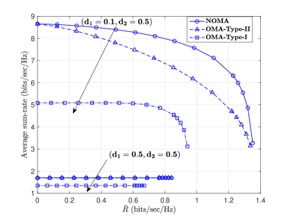
Figure 2: The average sum-rate of the system versus the minimum rate constraints under full CSIT.

Fig. 2 depicts the optimal trade-offs between the average sum-rate of the system and the minimum rate constraints under full CSIT, i.e., $\bar{R}$, achieved by NOMA and the OMA schemes with different distance settings. It is seen that with the near-far distance setting, NOMA outperforms OMA-Type-II transmission in most cases, while the gap shrinks when $\bar{R}$ is very little and/or approaches $\bar{R}_{\max}$, respectively. Moreover, both NOMA and OMA-Type-II achieve substantially larger optimal trade-off than OMA-Type-I, although OMA-Type-I is seen more robust against increase in $\bar{R}$. This is because OMA-Type-I is intrinsically of fairness in view of equal time/frequency assigned to each user irrespective of their CSI. It is also worth noting that when there is no difference between the two users in terms of large-scale fading, the average sum-rate versus min-rate trade-offs almost vanish, since the average sum-rate w/o the minimum rate constraint has already achieved certain fairness, i.e., $\mathbb{E}_{\nu}[R_{k}^{\rm NOMA}(\nu)]\approx\mathbb{E}_{\nu}[R_{\bar{k}}^{\rm NOMA}(\nu)]$ ($\mathbb{E}_{\nu}[R_{k}^{\rm OMA\text{-}II}(\nu)]\approx\mathbb{E}_{\nu}[R_{\bar{k}}^{\rm OMA\text{-}II}(\nu)]$) due to their statistically similar channel distribution.

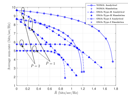
Figure 3: The average sum-rate of the system versus the minimum rate constraints under partial CSIT.

Fig. 3 shows the optimal trade-offs between the average sum-rate of the system versus the minimum rate constraints under partial CSIT, i.e., $\bar{R}^{\prime}$, achieved by various multiple access schemes with different APC. The optimal trade-off regions between the average-sum rate of the system and the fairness are expectedly seen to enlarge with increasing limit on the transmit power $\bar{P}$. While the superiority of the proposed power allocation policies for NOMA against OMA-Type-II is obviously seen, the contrast is more sharply observed for NOMA against OMA-Type-I in Fig.  2.

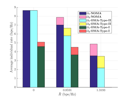
(a) Full CSIT.

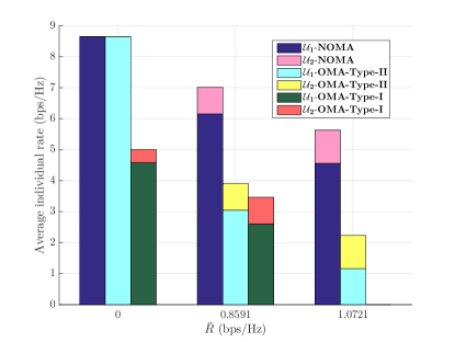
(b) Partial CSIT.

Figure 4: The average achievable rate allocation between the two users with different minimum rate requirements, under full and partial CSIT, respectively.

The comparison between the individual ergodic rate subject to varied minimum average rate constraints is demonstrated in Fig. 4(a) (Fig. 4(b)) for NOMA, OMA-Type-I, and OMA-Type-II, respectively, under full (partial) CSIT. First, we see that OMA-Type-II achieves almost the same ergodic rate for $\mathcal{U}_{1}$ as NOMA with $\mathcal{U}_{2}$’s ergodic rate both as little as zero, when there is no minimum rate requirement. This can be intuitively explained as follows. Since $\mathcal{U}_{1}$ is the near user who enjoys better CSI in most of the fading states, the optimal power policy that maximizes the average sum-rate for both NOMA and OMA-Type-II is to allocate power only to $\mathcal{U}_{1}$ in such states. Moreover, the advantage of NOMA begins promising when the system requires a larger $\bar{R}$ ($\bar{R}^{\prime}$), in that NOMA guarantees the minimum average rate achieved by $\mathcal{U}_{2}$ while keeping $\mathcal{U}_{1}$’s average rate the maximum.

V-B Delay-Limited Transmission

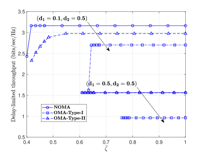
(a)

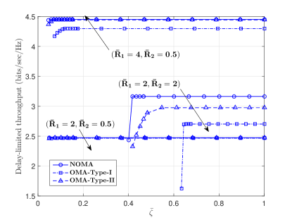
(b)

Figure 5: The DLT of the system versus the maximum permissive outage probability under full CSIT.

Fig. 5(a) shows the optimal trade-offs between the sum of DLT and the maximum permissive outage probability, i.e., $\bar{\zeta}$, under full CSIT given the same prescribed rate $\bar{R}_{k}=2$bits/sec/Hz for each user. It is seen that when the two users suffer from near-far unfairness, the optimum sum-DLT versus max-outage trade-off achieved by NOMA outperforms that achieved by OMA-Type-II and OMA-Type-I. However, this superiority almost disappears when $\mathcal{U}_{1}$ and $\mathcal{U}_{2}$ are both $0.5$km away from the BS. This is because in this case $g_{1}(\nu)\approx g_{2}(\nu)$ in most fading states, thanks to which the total amount of transmit power saved by NOMA tends to be less. Furthermore, no much trade-off is seen for the sum of DLT versus user fairness, as the two users hold similar chances to be the stronger user, and therefore when $\zeta_{k}^{\rm XX}$ is minimized, $\zeta_{\bar{k}}^{\rm XX}$ is nearly minimized as well, where $(\cdot)^{\rm XX}$ stands for ${\rm NOMA}$ or ${\rm OMA\text{-}Type\text{-}II}$.

On the other hand, in near-far channel conditions, the impact of different $\bar{R}_{k}$s on the optimum sum-DLT versus max-outage trade-off is demonstrated in Fig. 5(b). With the same intended rate $\bar{R}_{1}=\bar{R}_{2}=2$bits/sec/Hz, the optimum trade-off achieved by NOMA outperforms that achieved by the OMA schemes. By contrast, when $\bar{R}_{2}$ reduces to $0.5$bits/sec/Hz, the trade-off becomes trivial, since in this case the stronger user’s advantage in saving power is compromised by its higher target rate.

Figure 6: The DLT of the system versus the maximum permissive user outage probability under partial CSIT.

Fig. 6 shows the optimum sum-DLT versus max-outage trade-offs achieved by various schemes with different settings of $\bar{R}_{1}$ and $\bar{R}_{2}$. Unlike in Fig. 5(b), the superiority of NOMA over the other OMA schemes is significantly seen in Fig. 6. Moreover, the minimum max-outage achieved by NOMA is significantly lower than that attained by other schemes. For example, with $\bar{R}_{1}=\bar{R}_{2}=1$bist/sec/Hz, $\min\limits_{p_{s},p_{w}}\{\max\limits_{k}\zeta_{k}^{\prime\rm NOMA}\}$ falls below $0.47$ while that achieved by OMA-Type-I and OMA-Type-II is as large as about $0.49$ and $0.60$, respectively.

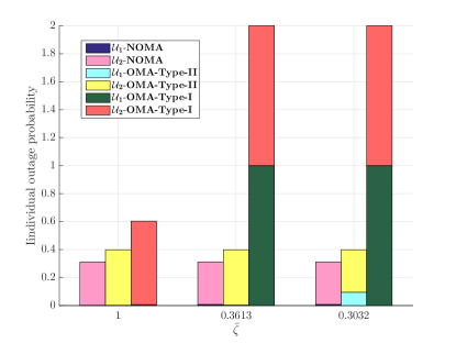
(a) Full CSIT.

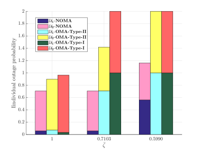
(b) Partial CSIT.

Figure 7: The DLT allocation between the two users with different maximum outage requirements, under full and partial CSIT.

The DLT allocation between the two users subject to different maximum permissive outage is reflected by their outage probability allocation in Fig. 7 under full and partial CSIT, respectively. Under full CSIT, it is seen from Fig. 7(a) that with $\bar{R}_{1}=\bar{R}_{2}=2$bits/sec/Hz and $\bar{P}=2$Watt, $\mathcal{U}_{1}$ achieves almost negligible outage while $\mathcal{U}_{2}$ can achieve an outage probability as low as $0.3032$ by NOMA. OMA-Type-II follows the same trend unless $\mathcal{U}_{1}$ has to claim more outage states to reserve power for $\mathcal{U}_{2}$’s transmission. $\mathcal{U}_{1}$’s outage probability compromised by satisfying a lower maximum outage constraint is larger in the case of partial CSIT than in the case of full CSIT.

VI Conclusion

In this paper, we have investigated the average sum-rate and/or the sum of DLT maximization for a two-user downlink NOMA over fading channels imposing QoS constraints on the worst user performance. Under full CSIT, the non-convex resource allocation problems have been solved using the technique of dual decomposition leveraging “time-sharing” conditions. Under partial CSIT, the individual ergodic rate and/or outage probability have been characterized in closed-form, based on which the optimal power policies have been numerically obtained. Simulation results have unveiled that the optimal NOMA-based power allocation schemes in general outperform the optimal OMA-based ones in terms of various throughput versus fairness trade-offs, especially when the two users’ channels experience contrasting fading gains.

Appendix A

As $p_{1}+p_{2}=\hat{P}$ is fixed, $\mathrm{(P1\text{-}OMA\text{-}II\text{-}sub)}$ reduces to the following problem irrespective of $\lambda$:

$$\mathop{\mathtt{Maximize}}_{p_{1}\geq 0,p_{2}\geq 0,\alpha_{1}} ~{}~{}(1+\delta)\alpha_{1}\log_{2}\left(1+\frac{p_{1}g_{1}}{\alpha_{1}}\right)+$$

$$~{}~{}(1+\mu)\alpha_{2}\log_{2}\left(1+\frac{p_{2}g_{2}}{\alpha_{2}}\right)$$

$$\mathtt{Subject\ to} ~{}~{}p_{1}+p_{2}\leq\hat{P},$$ (95a)

$$~{}~{}0\leq\alpha_{1}\leq 1,$$ (95b)

where $\alpha_{2}=1-\alpha_{1}$. Note that $=$ has been relaxed into $\leq$ in (95a), since it is easy to check that the above problem obtains its optimum value when (95a) is active.

To facilitate solving (95), we introduce a new Lagrangian multiplier $\lambda^{\prime}$ associated with the constraint (95a). Then given $\lambda^{\prime}$, we aim for maximizing the Lagrangian regarding Problem (95) as follows:

$$\mathop{\mathtt{Maximize}}_{p_{1}\geq 0,p_{2}\geq 0,\alpha_{1}} ~{}~{}~{}\bar{\mathcal{L}}_{1}^{\prime\rm OMA\text{-}II}(p_{1},p_{2},\alpha_{1},\lambda^{\prime})$$

$$\mathtt{Subject\ to} ~{}~{}~{}0\leq\alpha_{1}\leq 1,$$ (96a)

in which $\bar{\mathcal{L}}_{1}^{\prime\rm OMA\text{-}II}(p_{1},p_{2},\alpha_{1},\lambda^{\prime})=(1+\delta)\alpha_{1}\log_{2}(1+\frac{p_{1}g_{1}}{\alpha_{1}})+(1+\mu)(1-\alpha_{1})\log_{2}(1+\frac{p_{2}g_{2}}{1-\alpha_{1}})-\lambda^{\prime}(p_{1}+p_{2})$. It is worthy of noting that Problem (96) shares the same structure as $\mathrm{(P1\text{-}OMA\text{-}II\text{-}sub)}$ except that the constraint $p_{1}+p_{2}\leq\hat{P}$ is now removed. Therefore, the rationale behind solving it has been similarly given in the proof for Proposition III.2. As a result, given $\lambda^{\prime}$, the maximizer of $\bar{\mathcal{L}}_{1}^{\prime\rm OMA\text{-}II}(p_{1},p_{2},\alpha_{1},\lambda^{\prime})$ proves to be either $(0,(\frac{1+\mu}{\lambda^{\prime}\ln 2}-\frac{1}{g_{2}})^{+},0)$ or $((\frac{1+\delta}{\lambda^{\prime}\ln 2}-\frac{1}{g_{1}})^{+},0,1)$, i.e., alternative transmission. Therefore, by updating $\lambda^{\prime}$ via bi-section until (95a) is active, the optimal solution to Problem (95) ends up with $(0,\hat{P},0)$ or $(\hat{P},0,1)$ depending on which leads to a larger objective value. Hence, we complete the proof for Lemma III.2.

Appendix B

As the maximum of $\bar{\mathcal{L}}_{1}^{\rm OMA\text{-}II}(p_{1},p_{2},\alpha_{1})$ must be either at the stationary point or on the boundary of $\Psi$ as defined in Proposition III.1, the vertexes of $(0,0,0)$, $(0,\hat{P},0)$, and $(\hat{P},0,1)$ are included in (51) for sure.

As for another case that the maximum of $\bar{\mathcal{L}}_{1}^{\rm OMA\text{-}II}(p_{1},p_{2},\alpha_{1})$ is achieved on $p_{1}=0$, the corresponding optimum value of $\bar{\mathcal{L}}_{1}^{\rm OMA\text{-}II}(p_{1},p_{2},\alpha_{1})$ takes on $\bar{\mathcal{L}}_{1}^{\rm OMA\text{-}II}(0,c_{2},0)\mathbbm{1}_{c_{2}}$ because of the following reasons. Plugging $p_{1}=0$ into $\bar{\mathcal{L}}_{1}^{\rm OMA\text{-}II}(p_{1},p_{2},\alpha_{1})$, its derivative w.r.t $p_{2}$ and $\alpha_{1}$ are, respectively, expressed as:

$$\frac{\partial\bar{\mathcal{L}}_{1}^{\rm OMA\text{-}II}(p_{1},p_{2},\alpha_{1})}{p_{2}}= \frac{(1+\mu)\alpha_{2}g_{2}}{(\alpha_{2}+p_{2}g_{2})\ln 2}-\lambda,$$ (97)

$$\frac{\partial\bar{\mathcal{L}}_{1}^{\rm OMA\text{-}II}(p_{1},p_{2},\alpha_{1})}{\alpha_{1}}= \frac{(1+\mu)}{\ln 2}\bigg{[}-\ln\left(1+\frac{p_{2}g_{2}}{1-\alpha_{1}}\right)+$$

$$1-\frac{1}{1+p_{2}g_{2}\mathord{\left/\right.\kern-1.2pt}(1-\alpha_{1})}\bigg{]}.$$ (98)

It is then easily seen that the optimal $p_{2}$ admits the form of $p_{2}^{\ast}=[c_{2}(1-\alpha_{1})]_{0}^{\hat{P}}$. Further, $\bar{\mathcal{L}}_{1}^{\rm OMA\text{-}II}(0,p_{2},\alpha_{1})$ turns out to monotonically decrease w.r.t $\alpha_{1}$ by observing that the RHS of (98) is always negative in view of the inequality $1-\frac{1}{x}\leq\ln x$. Hence, $\alpha_{1}^{\ast}=0$, and $(0,c_{2},0)$ is the optimum iff $0\leq c_{2}\leq\hat{P}$, which leads to $\bar{\mathcal{L}}_{1}^{\rm OMA\text{-}II}(0,c_{2},0)\mathbbm{1}_{c_{2}}$. Similarly, $\bar{\mathcal{L}}_{1}^{\rm OMA\text{-}II}(c_{1},0,1)\mathbbm{1}_{c_{1}}$ can be justified considering another boundary of $p_{2}=0$.

At last, the reasons why the jointly stationary point (c.f. (44)) cannot be the optimal solution to $\mathrm{(P1\text{-}OMA\text{-}II\text{-}sub)}$ has been explained in Remark III.1.

Appendix C

$$\mathbb{E}_{\nu}[{R_{k}^{\prime\rm NOMA}(\nu)}]$$

$$=\Pr\{X\geq Y\}\mathbb{E}_{\nu}\left[{\left.{{{\log}_{2}}\left({1+{\Gamma_{k}}}\right)}\right|X\geq Y}\right]+$$

$$\ ~{}~{}\Pr\{X<Y\}\mathbb{E}_{\nu}\left[{\left.{{{\log}_{2}}\left({1+{\tilde{\Gamma}_{k}}}\right)}\right|X<Y}\right]$$

$$=\frac{1}{{\ln 2}}\Pr\{X\geq Y\}\int_{0}^{\infty}{\frac{{1-{F_{{\Gamma_{k|X\geq Y}}}}\left({{z}}\right)}}{{1+z}}}\mathrm{d}z+$$

$$\ ~{}~{}\frac{1}{{\ln 2}}\Pr\{X<Y\}\int_{0}^{\infty}{\frac{{1-{F_{{\tilde{\Gamma}_{k}|X<Y}}}}\left({{z}}\right)}{{1+z}}}\mathrm{d}z$$

$$\stackrel{{\scriptstyle\rm(a)}}{{=}}\frac{1}{{\ln 2}}\frac{{{\lambda_{k}}}}{{{\lambda_{k}}+{\lambda_{\bar{k}}}}}A_{1}+\frac{1}{{\ln 2}}B_{1}-\frac{1}{{\ln 2}}\frac{{{\lambda_{k}}}}{{{\lambda_{k}}+{\lambda_{\bar{k}}}}}C_{1},$$ (99)

where $A_{1}\triangleq\int_{0}^{\frac{{{p_{w}}}}{{{p_{s}}}}}{\frac{{{e^{-\left({{\lambda_{k}}+{\lambda_{\bar{k}}}}\right)\frac{{\sigma_{k}^{2}z}}{{{p_{w}}-{p_{s}}z}}}}}}{{1+z}}\mathrm{d}}z$, $B_{1}\triangleq\int_{0}^{\infty}{\frac{{{e^{-\frac{{{\lambda_{k}}\sigma_{k}^{2}}}{{{p_{s}}}}z}}}}{{1+z}}\mathrm{d}}z$, and $C_{1}\triangleq\int_{0}^{\infty}{\frac{{{e^{-\frac{{\left({{\lambda_{k}}+{\lambda_{\bar{k}}}}\right)\sigma_{k}^{2}}}{{{p_{s}}}}z}}}}{{1+z}}\mathrm{d}}z$. Since $\Pr\{X\geq Y\}=\frac{\lambda_{\bar{k}}}{\lambda_{k}+\lambda_{\bar{k}}}$, substituting (56) and (59) for $F_{\Gamma_{k}|X\geq Y}(z)$ and $F_{\tilde{\Gamma}_{k}|X<Y}(z)$ in (99), respectively, ${\rm(a)}$ is derived. Then after some manipulations, by applying [33, Eq. (3.352.4)], we have $A_{1}=f(\frac{{({{\lambda_{k}}+{\lambda_{\bar{k}}}})\sigma_{k}^{2}}}{{{p_{s}}}})-f(\frac{{({{\lambda_{k}}+{\lambda_{\bar{k}}}})\sigma_{k}^{2}}}{{{p_{s}}+{p_{w}}}})$. It also immediately follows that $B_{1}=-f(\frac{{{\lambda_{k}}\sigma_{k}^{2}}}{{{p_{s}}}})$ and $C_{1}=-f(\frac{{\left({{\lambda_{k}}+{\lambda_{\bar{k}}}}\right)\sigma_{k}^{2}}}{{{p_{s}}}})$. Plugging $A_{1}$, $B_{1}$ and $C_{1}$ into (99), Proposition III.3 is proved.

Appendix D

$$\mathbb{E}_{\nu}[R_{k}^{\prime\rm OMA\text{-}II}(\nu)]$$

$$=\Pr\{X\geq Y\}\mathbb{E}_{\nu}\left[{\left.\alpha_{k}{{{\log}_{2}}\left({1+{\Gamma_{k}}}\right)}\right|X\geq Y}\right]+$$

$$\ ~{}~{}\Pr\{X<Y\}\mathbb{E}_{\nu}\left[{\left.\alpha_{k}{{{\log}_{2}}\left({1+{\tilde{\Gamma}_{k}}}\right)}\right|X<Y}\right]$$

$$=\frac{\alpha_{k}}{{\ln 2}}\frac{\lambda_{\bar{k}}}{\lambda_{k}+\lambda_{\bar{k}}}\int_{0}^{\infty}{\frac{{1-{F_{{\Gamma_{k|X\geq Y}}}}\left({{z}}\right)}}{{1+z}}}\mathrm{d}z+$$

$$\ ~{}~{}\frac{\alpha_{k}}{{\ln 2}}\frac{\lambda_{k}}{\lambda_{k}+\lambda_{\bar{k}}}\int_{0}^{\infty}{\frac{{1-{F_{{\tilde{\Gamma}_{k}|X<Y}}}}\left({{z}}\right)}{{1+z}}}\mathrm{d}z$$

$$\stackrel{{\scriptstyle\rm(a)}}{{=}}-\frac{\alpha_{k}}{{\ln 2}}\frac{{{\lambda_{k}}}}{{{\lambda_{k}}+{\lambda_{\bar{k}}}}}A_{1}^{\prime}+\frac{\alpha_{k}}{{\ln 2}}B_{1}^{\prime}+\frac{\alpha_{k}}{{\ln 2}}\frac{{{\lambda_{k}}}}{{{\lambda_{k}}+{\lambda_{\bar{k}}}}}C_{1}^{\prime},$$ (100)

where $A_{1}^{\prime}\triangleq\int_{0}^{\infty}{\frac{{{e^{-\frac{{\left({{\lambda_{k}}+{\lambda_{\bar{k}}}}\right)\alpha_{k}\sigma_{k}^{2}}}{{{p_{s}}}}z}}}}{{1+z}}\mathrm{d}}z$, $B_{1}^{\prime}\triangleq\int_{0}^{\infty}{\frac{{{e^{-\frac{{{{\lambda_{k}}}\alpha_{k}\sigma_{k}^{2}}}{{{p_{s}}}}z}}}}{{1+z}}\mathrm{d}}z$, and $C_{1}^{\prime}\triangleq\int_{0}^{\infty}{\frac{{{e^{-\frac{{\left({{\lambda_{k}}+{\lambda_{\bar{k}}}}\right)\alpha_{k}\sigma_{k}^{2}}}{{{p_{w}}}}z}}}}{{1+z}}\mathrm{d}}z$, which are obtained by substituting (62) and (63) for ${F_{{\Gamma_{k|X\geq Y}}}}({{z}})$ and ${F_{{\tilde{\Gamma}_{k|X<Y}}}}({{z}})$, respectively. Then by directly applying [33, Eq. (3.352.4)], $A_{1}^{\prime}=-f(\frac{{\left({{\lambda_{k}}+{\lambda_{\bar{k}}}}\right)\alpha_{k}\sigma_{k}^{2}}}{{{p_{s}}}})$, $B_{1}^{\prime}=-f(\frac{{{{\lambda_{k}}}\alpha_{k}\sigma_{k}^{2}}}{{{p_{s}}}})$ and $C_{1}^{\prime}=-f(\frac{{\left({{\lambda_{k}}+{\lambda_{\bar{k}}}}\right)\alpha_{k}\sigma_{k}^{2}}}{{{p_{w}}}})$ are derived, which completes the proof for Proposition 64.

Appendix E

Following similar analysis as for Proposition IV.1, the minimum of $\bar{\mathcal{L}}_{2}^{\rm OMA\text{-}II}(p_{k},p_{\bar{k}},\alpha_{k})$ is obtained by comparing all possible combinations of outage occurrences for $\mathcal{U}_{k}$ and $\mathcal{U}_{\bar{k}}$ (c.f. Table II). In (77), $p_{i,k}$ and $p_{i,\bar{k}}$, $i=1,2,3,4$, are respectively the minimum power required to have both of the users suspend their transmission, only $\mathcal{U}_{k}$ or $\mathcal{U}_{\bar{k}}$ supported, and both of the users simultaneously served.

Appendix F

Note from Lemma IV.1 that to prove $P_{\rm O2}^{\ast}\geq P_{\rm N}^{\ast}$, it is sufficient to show that $\sum_{i=1}^{K}\frac{(2^{\frac{\bar{R}_{i}}{\alpha_{i}}}-1)\alpha_{i}}{g_{i}}\geq P_{\rm N}^{\ast}$ holds for any $\alpha_{i}$’s such that $\sum_{i=1}^{K}\alpha_{i}=1$. By variable transformation of $i\leftarrow(K-i)$, it follows that $P_{\rm N}^{\ast}=\sum_{i=1}^{K}\frac{(2^{\bar{R}_{i}}-1)2^{\sum_{l=i+1}^{K}\bar{R}_{l}}}{g_{i}}$.

First, denoting $(2^{\frac{\bar{R}_{i}}{\alpha_{i}}}-1)\alpha_{i}$ by $a_{i}$, and $(2^{\bar{R}_{i}}-1)2^{\sum_{l=i+1}^{K}\bar{R}_{l}}$ by $b_{i}$, $\forall i$, we prove that $\sum_{i=j}^{K}a_{i}\geq\sum_{i=j}^{K}b_{i}$ holds for $\forall j=1,\ldots,K$. Expand $\sum_{i=j}^{K}b_{i}$ as follows:

$$\left\{\begin{array}[]{cl}2^{\sum_{l=j}^{K}\bar{R}_{l}}-2^{\sum_{l=j+1}^{K}\bar{R}_{l}},&i=j\\ 2^{\sum_{l=j+1}^{K}\bar{R}_{l}}-2^{\sum_{l=j+2}^{K}\bar{R}_{l}},&i=j+1\\ \vdots&i=j+2,\ldots,K-1\\ 2^{\bar{R}_{K}}-1.&i=K\end{array}\right.$$ (105)

By summing-up the LHS of (105), $\sum_{i=j}^{K}b_{i}$ is simplified as $2^{\sum_{i=j}^{K}\bar{R}_{i}}-1$. Defining a function $f_{0}(x)=2^{x}-1$, let $x_{i}=0$ for $i=1,\ldots,j-1$, and $x_{i}=\frac{\bar{R}_{i}}{\alpha_{i}}$ for $i=j,\ldots,K$. Then by applying Jensen’s inequality due to the convexity of $f_{0}(x)$, it follows that

$$\sum_{i=j}^{K}a_{i}=\sum_{i=1}^{K}\alpha_{i}f_{0}(x_{i})\\ \geq f_{0}\left(\sum_{i=1}^{K}\alpha_{i}x_{i}\right)=f_{0}\left(\sum_{i=j}^{K}\alpha_{i}x_{i}\right)=\sum_{i=j}^{K}b_{i}.$$ (106)

Next, define $\frac{1}{g_{i}}$ by $c_{i}$, $\forall i$, it is easily verified that $0<c_{1}\leq c_{2}\leq\ldots\leq c_{K}$. By applying [15, Lemma 4], we conclude that $\sum_{i=1}^{K}\frac{(2^{\frac{\bar{R}_{i}}{\alpha_{i}}}-1)\alpha_{i}}{g_{i}}\geq\sum_{i=1}^{K}\frac{(2^{\bar{R}_{i}}-1)2^{\sum_{l=i+1}^{K}\bar{R}_{l}}}{g_{i}}=P_{\rm N}^{\ast}$, which completes the proof for Lemma IV.1.

Appendix G

The piece-wise presentation of $\mathbb{E}_{\nu}[X_{k}^{\prime\rm NOMA}(\nu)]$ is caused by the range of the parameters. To illustrate as an example, take the second term of (79) as an example and express it as follows:

$$\Pr\bigg{\{}\log_{2}\left(1+\frac{p_{s}X}{\sigma_{k}^{2}}\right)<\bar{R}_{k},\log_{2}\left(1+\frac{p_{w}X}{p_{s}X+\sigma_{k}^{2}}\right)\geq\bar{R}_{\bar{k}},$$

$$\ ~{}~{}~{}~{}X>Y\bigg{\}}$$

$$=\Pr\left\{X<\varepsilon_{k,1},\left(p_{w}-p_{s}\tau_{\bar{k}}\right)X\geq\sigma_{k}^{2}\tau_{\bar{k}},X>Y\right\}$$

$$=\left\{\kern-4.0pt\begin{array}[]{l}\Pr\left\{X<\varepsilon_{k,1},X\geq\varepsilon_{k,4},X>Y\right\},\ {\rm if}\ \frac{p_{s}}{p_{w}}<\frac{1}{\tau_{\bar{k}}},\\ 0,\ {\rm otherwise.}\end{array}\right.$$ (109)

Further, the first case in (109) implies the following two sub-cases:
Case 1: $\frac{p_{s}}{p_{w}}<\min\left\{\frac{\tau_{k}}{\tau_{\bar{k}}(\tau_{k}+1)},\frac{1}{\tau_{\bar{k}}}\right\}$

$$\Pr\left\{X<\varepsilon_{k,1},X\geq\varepsilon_{k,4},X>Y\right\}=\\ \Pr\left\{\varepsilon_{k,4}\leq X<\varepsilon_{k,1},X>Y\right\};$$ (110)

Case 2: $\frac{p_{s}}{p_{w}}\geq\min\left\{\frac{\tau_{k}}{\tau_{\bar{k}}(\tau_{k}+1)},\frac{1}{\tau_{\bar{k}}}\right\}$

$$\Pr\left\{X<\varepsilon_{k,1},X\geq\varepsilon_{k,4},X>Y\right\}=0.$$ (111)

Hence, in the case of $\frac{p_{s}}{p_{w}}<\min\{\tau_{k}\mathord{\left/\right.\kern-1.2pt}\tau_{\bar{k}}(\tau_{k}+1),1\mathord{\left/\right.\kern-1.2pt}\tau_{\bar{k}}\}$, after some manipulations, the second term of (79) turns out to be $e^{-\lambda_{k}\varepsilon_{k,4}}-e^{-\lambda_{k}\varepsilon_{k,1}}+\frac{\lambda_{k}}{\lambda_{k}+\lambda_{\bar{k}}}(e^{-(\lambda_{k}+\lambda_{\bar{k}})\varepsilon_{k,1}}-e^{-(\lambda_{k}+\lambda_{\bar{k}})\varepsilon_{k,4}})$ (c.f. (110)), and otherwise zero (c.f. (111)). By analogy, the first and the third term of (79) can also be analysed piece-wisely. Finally, we arrive at (86) combining all possible cases.

References

• [1] H. Xing, Y. Liu, A. Nallanathan, and Z. Ding, “Sum-rate maximization guaranteeing user fairness for NOMA in fading channels,” in Proc. IEEE Wireless Communications and Networking Conference (WCNC), Barcelona, Spain, Apr. 2018.
• [2] Y. Saito, Y. Kishiyama, A. Benjebbour, T. Nakamura, A. Li, and K. Higuchi, “Non-orthogonal multiple access (NOMA) for cellular future radio access,” in Proc. IEEE Vehicular Technology Conference (VTC Spring), Dresden, Germany, June 2013.
• [3] H. Xie, B. Wang, F. Gao, and S. Jin, “A full-space spectrum-sharing strategy for massive MIMO cognitive radio systems,” IEEE J. Sel. Areas Commun., vol. 34, no. 10, pp. 2537–2549, Oct. 2016.
• [4] L. Dai, B. Wang, Y. Yuan, S. Han, C. l. I, and Z. Wang, “Non-orthogonal multiple access for 5G: solutions, challenges, opportunities, and future research trends,” IEEE Commun. Mag., vol. 53, no. 9, pp. 74–81, Sept. 2015.
• [5] Z. Ding, Y. Liu, J. Choi, Q. Sun, M. Elkashlan, C.-L. I, and H. V. Poor, “Application of non-orthogonal multiple access in LTE and 5G networks,” IEEE Commun. Mag., vol. 55, no. 2, pp. 185–191, Feb. 2017.
• [6] 3rd Generation Partnership Project (3GPP), “Study on downlink multiuser superposition transmission for LTE,” Mar. 2015.
• [7] L. Zhang, W. Li, Y. Wu, X. Wang, S. I. Park, H. M. Kim, J. Y. Lee, P. Angueira, and J. Montalban, “Layered-division-multiplexing: theory and practice,” IEEE Trans. on Broadcast., vol. 62, no. 1, pp. 216–232, Mar. 2016.
• [8] Z. Ding, Z. Yang, P. Fan, and H. V. Poor, “On the performance of non-orthogonal multiple access in 5G systems with randomly deployed users,” IEEE Signal Process. Lett., vol. 21, no. 12, pp. 1501–1505, 2014.
• [9] J. Choi, “Non-orthogonal multiple access in downlink coordinated two-point systems,” IEEE Commun. Lett., vol. 18, no. 2, pp. 313–316, Feb. 2014.
• [10] W. Shin, M. Vaezi, B. Lee, D. J. Love, J. Lee, and H. V. Poor, “Coordinated beamforming for multi-cell MIMO-NOMA,” IEEE Commun. Lett., vol. 21, no. 1, pp. 84–87, Jan. 2017.
• [11] Z. Ding, M. Peng, and H. V. Poor, “Cooperative non-orthogonal multiple access in 5G systems,” IEEE Commun. Lett., vol. 19, no. 8, pp. 1462–1465, Aug. 2015.
• [12] Y. Liu, Z. Ding, M. Elkashlan, and H. V. Poor, “Cooperative non-orthogonal multiple access with simultaneous wireless information and power transfer,” IEEE J. Sel. Areas Commun., vol. 34, no. 4, pp. 938–953, Apr. 2016.
• [13] S. Timotheou and I. Krikidis, “Fairness for non-orthogonal multiple access in 5G systems,” IEEE Signal Process. Lett., vol. 22, no. 10, pp. 1647–1651, Oct. 2015.
• [14] Y. Liu, M. Elkashlan, Z. Ding, and G. K. Karagiannidis, “Fairness of user clustering in MIMO non-orthogonal multiple access systems,” IEEE Commun. Lett., vol. 20, no. 7, pp. 1465–1468, Jul. 2016.
• [15] Z. Chen, Z. Ding, X. Dai, and R. Zhang, “An optimization perspective of the superiority of NOMA compared to conventional OMA,” IEEE Trans. Signal Process., vol. 65, no. 19, pp. 5191–5202, Oct 2017.
• [16] B. Di, L. Song, and Y. Li, “Sub-channel assignment, power allocation, and user scheduling for non-orthogonal multiple access networks,” IEEE Trans. Wireless Commun., vol. 15, no. 11, pp. 7686–7698, Nov. 2016.
• [17] Y. Sun, D. W. K. Ng, Z. Ding, and R. Schober, “Optimal joint power and subcarrier allocation for full-duplex multicarrier non-orthogonal multiple access systems,” IEEE Trans. Commun., vol. 65, no. 3, pp. 1077–1091, Mar. 2017.
• [18] L. Li and A. Goldsmith, “Capacity and optimal resource allocation for fading broadcast channels .I. ergodic capacity,” IEEE Trans. Inf. Theory, vol. 47, no. 3, pp. 1083–1102, Mar. 2001.
• [19] ——, “Capacity and optimal resource allocation for fading broadcast channels .II. outage capacity,” IEEE Trans. Inf. Theory, vol. 47, no. 3, pp. 1103–1127, Mar. 2001.
• [20] H. Xing, L. Liu, and R. Zhang, “Secrecy wireless information and power transfer in fading wiretap channel,” IEEE Trans. Veh. Technol., vol. 65, no. 1, pp. 180–190, Jan. 2016.
• [21] N. Jindal and A. Goldsmith, “Capacity and optimal power allocation for fading broadcast channels with minimum rates,” IEEE Trans. Inf. Theory, vol. 49, no. 11, pp. 2895–2909, Nov. 2003.
• [22] D. Hughes-Hartogs, “The capacity of a degraded spectral gaussian broadcast channel,” Ph.D. dissertation, Inform. Syst. Lab., Ctr. Syst. Res., Stanford Univ., Stanford, CA, Jul. 1975.
• [23] Study on Downlink Multiuser Superposition Transmission (MUST) for LTE (Release 13), 3GPP document TR 36.859, Dec. 2015.
• [24] Y. Wu, C. K. Wen, C. Xiao, X. Gao, and R. Schober, “Linear precoding for the MIMO multiple access channel with finite alphabet inputs and statistical CSI,” IEEE Trans. Wireless Commun., vol. 14, no. 2, pp. 983–997, Feb. 2015.
• [25] Z. Dong, H. Chen, J. K. Zhang, and L. Huang, “On non-orthogonal multiple access with finite-alphabet inputs in Z-channels,” IEEE J. Sel. Areas Commun., vol. 35, no. 12, pp. 2829–2845, Dec. 2017.
• [26] S. V. Hanly and D. N. C. Tse, “Multiaccess fading channels. ii. delay-limited capacities,” IEEE Trans. Inf. Theory, vol. 44, no. 7, pp. 2816–2831, Nov 1998.
• [27] H. Tabassum, E. Hossain, and J. Hossain, “Modeling and analysis of uplink non-orthogonal multiple access in large-scale cellular networks using Poisson cluster processes,” IEEE Trans. Commun., vol. 65, no. 8, pp. 3555–3570, Aug. 2017.
• [28] W. Yu and R. Lui, “Dual methods for nonconvex spectrum optimization of multicarrier systems,” IEEE Trans. Commun., vol. 54, no. 7, pp. 1310–1322, July 2006.
• [29] R. T. Rockafellar, Convex Analysis.   Princeton Univ. Press, 1997.
• [30] S. Boyd, “Lecture notes for EE364b: Convex Optimization II.” [Online]. Available: https://stanford.edu/class/ee364b/lectures.html
• [31] Y. Liu, Z. Ding, M. Elkashlan, and J. Yuan, “Non-orthogonal multiple access in large-scale underlay cognitive radio networks,” IEEE Trans. Veh. Technol., vol. 65, no. 12, pp. 10 152–10 157, Dec. 2016.
• [32] M. Abramowitz and I. A. Stegun, Handbook of Mathematical Functions: with Formulas, Graphs, and Mathematical Tables, 9th ed.   Mineola, NY, USA: Dover Publication, Inc., 1972.
• [33] I. S. Gradshteyn and I. M. Ryzhik, Table of Integrals, Series and Products, 6th ed.   New York, NY, USA: Academic Press, 2000.