Quantum metrology beyond the classical limit under the effect of dephasing

Abstract

Quantum sensors have the potential to outperform their classical counterparts. For classical sensing, the uncertainty of the estimation of the target fields scales inversely with the square root of the measurement time T. On the other hand, by using quantum resources, we can reduce this scaling of the uncertainty with time to $1/T$. However, as quantum states are susceptible to dephasing, it has not been clear whether we can achieve sensitivities with a scaling of $1/T$ for a measurement time longer than the coherence time. Here, we propose a scheme that estimates the amplitude of globally applied fields with the uncertainty of $1/T$ for an arbitrary time scale under the effect of dephasing. We use one-way quantum computing based teleportation between qubits to prevent any increase in the correlation between the quantum state and its local environment from building up and have shown that such a teleportation protocol can suppress the local dephasing while the information from the target fields keeps growing. Our method has the potential to realize a quantum sensor with a sensitivity far beyond that of any classical sensor.

It is well known that two-level systems are attractive candidates with which to realize ultrasensitive sensors as the frequency of the qubit can be shifted by coupling it to a target field. Such a frequency shift induces a relative phase between the qubits basis states which can be simply measured in a Ramsey type experiment. This method has been used to measure magnetic fields, electric fields, and temperature. Budker and Romalis (2007); Balasubramanian and et al (2008); Maze and et al (2008); Degen et al. (2016). With the typical classical sensor measurement devices (including SQUID’s Simon (1999), Hall sensors Chang et al. (1992), and force sensors Poggio and Degen (2010)), the uncertainty in the estimation of the target fields scales as $1/\sqrt{T}$ with a total measurement time $T$. This scaling is considered classical Huelga et al. (1997). With a qubit-based sensor using a Ramsey type measurement, the readout signal is periodic against the amplitude of the target fields. So, unless the range of the target fields is known, the interaction time with the target fields should be limited, which reduces the sensitivity. In this case, the sensitivity decreases as $1/t\sqrt{N}$ by performing $N$ repetitions with a short sensing time $t$. This sensitivity can be rewritten as $1/\sqrt{Tt}$ if fast qubit control is available. Although one could achieve the uncertainty with $1/T$ by setting $t=T$ with the knowledge of the target field range, a dynamic range, which allows us to estimate the fields unambiguously, becomes small due to the periodic structure of the readout signal. Fortunately, there is an ingenious way to improve the dynamic range by using a feedback control of the qubit Said et al. (2011); Higgins et al. (2007). Actually, several experimental demonstrations have shown a sensitivity that scales as $1/T$ with the high-dynamic range Higgins et al. (2007); Waldherr et al. (2012). However, as quantum states are susceptible to decoherence, it has generally been considered that such a scaling $1/T$ can only be realized if the measurement time $T$ is much shorter than the coherence time Demkowicz-Dobrzanski et al. (2012); Said et al. (2011). Recently several approaches have been proposed and demonstrated that use quantum error correction Gottesman (2009) and dynamical decoupling Viola et al. (1999); Taylor et al. (2008); De Lange et al. (2011) to circumvent this limitation. Using quantum error correction, we can measure the amplitude of the target field with an uncertainty scaling as $1/T$ under the effect of specific decoherence such as bit flip errors Dür et al. (2014); Herrera-Martí et al. (2015); Arrad et al. (2014); Kessler et al. (2014); Cohen et al. (2016); Unden et al. (2016); Sisi and et al (2017), while dynamical decoupling makes it possible to estimate the frequency of time-oscillating fields with sensitivity beyond the classical limit on time scale longer than the coherence time Schmitt and et al (2017); Boss et al. (2017). However, there is currently no known metrological scheme to achieve with an uncertainty of $1/T$ when measuring the amplitude of target fields with dephasing.

In this letter, we propose a scheme for measuring the amplitude of target fields with an uncertainty of $1/T$ under the effect of dephasing. We will use a similar concept to the quantum Zeno effect (QZE) Misra and Sudarshan (1977); Itano et al. (1990); Facchi et al. (2001). For shorter time scales than the correlation time of the environment $\tau_{c}$, the interaction with the environment induces a quadratic decay rate that is much slower than the typical exponential decay Nakazato et al. (1996). Frequent measurements can be used to reset the correlation with the environment and so keep this state in the initial quadratic decay region, which suppresses the decoherence Misra and Sudarshan (1977); Itano et al. (1990); Facchi et al. (2001). However, if we naively apply the QZE to quantum metrology, the frequent measurements freeze all the dynamics so that the quantum states cannot acquire any information from the target fields. Instead, we use quantum teleportation (QT) based on concepts taken from one-way quantum computation Raussendorf and Briegel (2001); Barjaktarevic et al. (2005); Silva et al. (2007); Olmschenk et al. (2009); Baur et al. (2012) to reset the correlation between the system and the environment Averin et al. (2016). If we transfer the quantum states to a new site, we can prevent any increase in the correlation between the system and environment in the previous site, and the quantum state are then only affected by a slow quadratic decay due to the local environment in the new site. This noise suppression with a qubit motion using a concept drawn from QT has been proposed and demonstrated by using superconducting qubits Averin et al. (2016). The crucial idea in this paper is to use this one-qubit teleportation-based noise suppression for quantum metrology. Interestingly, although the QT protocol eliminates the deterioration effect caused by the dephasing from the local environment, we can accumulate the phase information from the global target fields during this protocol. We have shown that, as long as nearly perfect QT is available, we can achieve a sensor with the uncertainty scaling $1/T$ with dephasing. Moreover, we have found that, even when the QT is moderately noisy, the sensitivity of our protocol is superior to that of the standard Ramsey measurement.

Noise and its suppression.– Our system and the environment in this situation can be described by a Hamiltonian of the form $H=H_{\rm{S}}+H_{\rm{I}}+H_{\rm{E}}$ Hornberger (2009) where $H_{\rm{S}}=\sum_{j=1}^{L}\frac{\omega}{2}\sigma^{(j)}_{z}\otimes\openone^{(j)}_{\rm{E}}$ ($H_{\rm{E}}=\sum_{j=1}^{L}\openone^{(j)}_{\rm{S}}\otimes C_{j}$) denotes the system (environmental) Hamiltonian while $H_{\rm{I}}=\sum_{j=1}^{L}\lambda\sigma^{(j)}_{z}\otimes B_{j}$ denotes the interaction between the system and the environment. Here $\sigma^{(j)}_{z}$ is the usual Pauli Z operator of the $j$-th qubit with frequency $\omega$, while $B_{j}$ and $C_{j}$ denote the environmental operator at that $j$-th site. $\hat{\openone}^{(j)}_{\rm{S}}$ ($\hat{\openone}^{(j)}_{\rm{E}}$) denotes an identity operator for the system (environment). Furthermore, we set $\hbar=1$. In an interaction picture, we have $H_{\rm{I}}(t)=\lambda\sum_{j=1}^{L}\sigma^{(j)}_{z}\otimes\tilde{B}_{j}(t)$ where $\tilde{B}_{j}(t)=e^{iH_{\rm{E}}t}B_{j}e^{-iH_{\rm{E}}t}$. The separable initial state is given as $\rho(0)=\bigotimes_{j=1}^{L}(\rho^{(j)}_{\rm{S}}(0)\otimes\rho^{(j)}_{\rm{E}})$. where we have assumed $\rho^{(j)}_{\rm{E}}$ is in thermal equilibrium ($[\rho^{(j)}_{\rm{E}},H_{\rm{E}}]=0$) and our noise is non-biased (${\rm{Tr}}[\rho^{(j)}_{\rm{E}}B_{j}]=0$) for all $j$. If the initial state is separable, we consider the first site by tracing out the others. Solving Schrodinger’s equation gives

$$\rho^{(1)}_{\rm{I}}(\tau)\simeq\rho^{(1)}(0)-i\lambda\int_{0}^{\tau}dt^{\prime}[\sigma^{(1)}_{z}\otimes\tilde{B}_{1}(t^{\prime}),\rho^{(1)}(0)]$$

$$-\lambda^{2}\int_{0}^{\tau}\int_{0}^{t^{\prime}}dt^{\prime}dt^{\prime\prime}[\sigma^{(1)}_{z}\otimes\tilde{B}_{1}(t^{\prime}),[\sigma^{(1)}_{z}\otimes\tilde{B}_{1}(t^{\prime\prime}),\rho^{(1)}(0)]]$$

using a second order perturbation expansion in $\lambda$ Hornberger (2009). Tracing out the environment, we have

$$\rho^{(1)}_{\rm{S}}(\tau) \simeq \rho^{(1)}_{\rm{S}}(0)$$

$$-\lambda^{2}\int_{0}^{\tau}\int_{0}^{t^{\prime}}dt^{\prime}dt^{\prime\prime}C^{(1)}_{t^{\prime}-t^{\prime\prime}}\left[\hat{\sigma}^{(1)}_{z},\left[\hat{\sigma}^{(1)}_{z},\rho^{(1)}_{\rm{S}}(0)\right]\right]$$

where we define the correlation function of the environment as $C^{(1)}_{t^{\prime}-t^{\prime\prime}}\equiv\frac{1}{2}{\rm{Tr}}[(\tilde{B}_{1}(t^{\prime})\tilde{B}_{1}(t^{\prime\prime})+\tilde{B}_{1}(t^{\prime\prime})\tilde{B}_{1}(t^{\prime}))\rho^{(1)}_{\rm{E}}]$. If we are interested in a time scale much shorter than the correlation time of the environment, we can approximate the correlation function as $C^{(1)}_{t^{\prime}-t^{\prime\prime}}\simeq C^{(1)}_{0}$. For most solid state systems, this is readily satisfied as the environment correlation time is much longer than the coherence time of the qubit De Lange et al. (2010); Yoshihara et al. (2006); Kakuyanagi et al. (2007); Kondo et al. (2016), and so this condition is readily satisfied for many systems. In such a case $\rho^{(1)}_{\rm{S}}(\tau)\simeq(1-\epsilon_{\tau})U_{1,\tau}\rho^{(1)}_{\rm{S}}(0)U_{1,\tau}^{\dagger}+\epsilon_{\tau}\hat{\sigma}^{(1)}_{z}U_{1,\tau}\rho^{(1)}_{\rm{S}}(0)U_{1,\tau}^{\dagger}\sigma^{(1)}_{z}$ with $U_{j,\tau}=e^{-{i\omega\tau}\hat{\sigma}^{(j)}_{z}/2}$ specifying the unitary operator for a site $j$ and $\epsilon_{\tau}=\lambda^{2}C_{0}\tau^{2}$ denoting the error rate for $\lambda^{2}C_{0}\tau^{2}\ll 1$. Since the error rate has a quadratic form in time $t$, the decoherence effect is negligible for short time scales $t\ll{1}/{\lambda\sqrt{C_{0}}}$. This has been discussed in the field of the QZE Misra and Sudarshan (1977); Itano et al. (1990); Facchi et al. (2001). On the other hand, if we consider longer time scales of $t>{1}/{\lambda\sqrt{C_{0}}}$ with the same environment, error accumulation will destroy the quantum coherence of the qubit.

Let us now describe the noise suppression technique using QT. It begins with free evolution of the qubit for a time $\tau=t/n$ (where $t$ is the total time and $n$ is the number of times QT is to be performed). After this, QT transports $\rho^{(1)}_{\rm{S}}$ to site $2$. The quantum state starts interacting with a new local environment described by a density matrix $\rho^{(2)}_{\rm{E}}$. The error rate will be suppressed due to the quadratic decay Averin et al. (2016). Performing QT $n$ times (each time to a fresh qubit) yields $\rho^{(n)}_{\rm{S}}(t)\simeq(1-\frac{\lambda^{2}C_{0}t^{2}}{n})U_{n,t}\rho_{\rm{S}}(0)U^{\dagger}_{n,t}+\frac{\lambda^{2}C_{0}t^{2}}{n}\hat{\sigma}_{z}U^{\dagger}_{n,t}\rho_{\rm{S}}(0)U^{\dagger}_{n,t}\sigma_{z}$ at site $n$. For a large $n$ this approaches the pure state $\rho_{\rm{S}}(t)\simeq U_{n,t}\rho_{\rm{S}}(0)U^{\dagger}_{n,t}$, and so our approach can suppress dephasing.

Definition of parameters.– Here, we discuss the key parameters that we will use in our scheme. We define $L$ and $M$ as the total number of the probe qubits and the size of the entangled state. In our scheme, there are three time scales, $\tau\ll t\ll T$. The interaction time between teleportations is denoted $\tau$. This interaction is repeated $n$ times between the state preparation and measurement, giving a total time denoted $t=n\tau$. The whole procedure including preparation and measurement is repeated $N$ times, giving a total interaction time $T$. As regards the dephasing model, although our general approach described above uses a perturbative analysis typically valid for a short time scale, we need to examine the dynamics of our system for arbitrary time scales. So we will consider a more specific noise model that is given by $\hat{\mathcal{E}}_{j}(\rho^{(j)}_{\rm{S}}(\tau))=\frac{1+e^{-\gamma^{2}\tau^{2}}}{2}U_{j,\tau}\rho^{(j)}_{\rm{S}}(0)U_{j,\tau}^{\dagger}+\frac{1-e^{-\gamma^{2}\tau^{2}}}{2}\hat{\sigma}^{(j)}_{z}U_{j,\tau}\rho^{(j)}_{\rm{S}}(0)U_{j,\tau}^{\dagger}\sigma^{(j)}_{z}$ at the site $j$ during the evolution for a time $\tau=t/n$ (with $\gamma$ representing the dephasing rate). This model is consistent with the general results described above when we choose $\gamma=\sqrt{2\lambda^{2}C_{0}}$ (See the supplementary materials). Typical dephasing models Palma et al. (1996); De Lange et al. (2010); Kakuyanagi et al. (2007); Yoshihara et al. (2006) show this behavior if the correlation time of the environment is much longer than the dephasing time. If we consider a state $\rho$ composed of $M$ qubits, the noise channel during the time evolution of $\tau$ is described as $\hat{\mathcal{E}}_{1}\hat{\mathcal{E}}_{2}\cdots\hat{\mathcal{E}}_{M}(\rho)$. We consider GHZ states $|\psi^{{\rm{(GHZ)}}}\rangle=\frac{1}{\sqrt{2}}\left[\bigotimes_{j=1}^{M}|0\rangle_{j}+\bigotimes_{j=1}^{M}|1\rangle_{j}\right]$ as a metrological resource Huelga et al. (1997); Shaji and Caves (2007); Bohmann et al. (2015). For a given $L$ qubits, we create GHZ states with a size of $M$ qubits, and the number of the GHZ states is ${L}/{M}$. In realistic situations, there will be errors caused during the QT operations, and so we consider an imperfect QT. If we teleport a state $\rho_{1}$ from $j=1,2,\cdots,M$ sites to $j^{\prime}=1+M,2+M,\cdots,2M$ sites, we obtain a state of $\rho^{\prime}_{2}=(1-p)^{M}\rho_{2}+(1-(1-p)^{M})\rho^{(\rm{error})}_{2}$ where $p$ is the error rate on a single qubit, $\rho_{2}$ is the ideal state (that we could obtain by a perfect QT), and $\rho^{(\rm{error})}_{2}=\frac{1}{2}(\bigotimes_{j=1+M}^{2M}|0\rangle_{j}\langle 0|+\bigotimes_{j=1+M}^{2M}|1\rangle_{j}\langle 1|)$ is the dephased state.

	General form of sensitivity	Perfect QT	Short T imperfect QT	Long T imperfect QT
Entangled sensor	$\delta\omega\simeq\frac{{\rm{Exp}}[M\gamma^{2}t^{2}/n]}{(1-p)^{M(n-1)}\sqrt{MLTt}}$	$\delta\omega\simeq\frac{{\rm{Exp}[1/4]}}{T\sqrt{ML}}$	$\delta\omega\simeq\frac{{\rm{Exp}[1/4]}}{T\sqrt{ML}}$ for $T\ll\frac{1}{\sqrt{p}\gamma M}$	$\delta\omega\simeq 2^{\frac{3}{4}}\sqrt{\frac{e\sqrt{p}\gamma}{TL}}$ for $T\gg\frac{1}{\sqrt{p}\gamma M}$
Separable sensor	$\delta\omega\simeq\frac{{\rm{Exp}}[\gamma^{2}t^{2}/n]}{(1-p)^{(n-1)}\sqrt{LTt}}$	$\delta\omega\simeq\frac{{\rm{Exp}[1/4]}}{T\sqrt{L}}$	$\delta\omega\simeq\frac{{\rm{Exp}[1/4]}}{T\sqrt{L}}$ for $T\ll\frac{1}{\sqrt{p}\gamma}$	$\delta\omega\simeq 2\sqrt{\frac{e\sqrt{p}\gamma}{TL}}$ for $T\gg\frac{1}{\sqrt{p}\gamma}$

Table 1: Performance of our teleportation based scheme with $L$ qubits for a given time $T$. Except with the general form, we show optimized sensitivity by choosing a suitable interaction time ($t$) and the QT number ($n$). The uncertainty of the standard Ramsey scheme is given as $\delta\omega_{{\rm{R}}}=e^{{1}/{4}}\sqrt{\gamma}/\sqrt{TL}$. With imperfect quantum teleportation that has an error rate of $p$, we can achieve a sensitivity scaling as $1/T$ using separable states (entangled states with a size $M$) for a short time scale of $T\ll 1/\sqrt{p}\gamma$ ($T\ll 1/\sqrt{p}\gamma M$). For a longer time scale, if accurate quantum teleportation is available ($p\ll 1$), the sensitivity of our scheme can be still better than the sensitivity of the standard Ramsey scheme. It is worth mentioning that, for the general form, perfect QT, and short T imperfect QT, the sensitivity of the separable sensor can be simply obtained by setting $M=1$ in that of the entangled sensor.

Quantum metrology with QT.– Here, we focus on using the QT scheme to enable quantum metrology with an uncertainty scaling as $1/T$. Consider the situation in which the qubit frequency $\omega$ is shifted depending on the amplitude of the target fields, and so measurement of the qubit’s frequency shift allows us to infer the amplitude of the target field. Such a qubit frequency shift is estimated from the relative phase between quantum states. The key idea is to use the QT in a ring arrangement with $2L$ qubits where each qubit has a tunable interaction with another qubit. Half of the qubits are used to probe the target fields while the remaining qubits are used as an ancilla for QT. The QT is accomplished by implementing a control-phase gate between a probe qubit and an ancilla qubit, followed by a $\hat{\sigma}_{x}$ measurement on the probe qubit (and single qubit corrections depending on the measurement result). This QT approach has been widely used in one-way quantum computation Raussendorf and Briegel (2001); Browne and Briegel (2006).

Scheme with entanglement.– Our scheme for measuring the amplitude of the target fields is as follows: First, we prepare GHZ states of $\bigotimes_{k=0}^{\frac{L}{M}-1}|\psi^{{\rm{(GHZ)}}}_{k}\rangle$ between the probe qubits where $|\psi^{{\rm{(GHZ)}}}_{k}\rangle=\frac{1}{\sqrt{2}}\left[\bigotimes_{j=1+2kM}^{M+2kM}|0\rangle_{j}+\bigotimes_{j=1+2kM}^{M+2kM}|1\rangle_{j}\right]$ for $k=0,1,\cdots,(\frac{L}{M}-1)$, while the other qubits (which we call ancillary qubits) are prepared in $|0\rangle$. Second we let the state evolve for time $\tau={t}/{n}$ and then teleport the state of the probe qubit at the site $j$ to another site $j+M$. We assume that our gate operations are much faster than $\tau$. Third, we repeat the second step $(n-1)$ times, while in the fourth step we let this state evolve for time $\tau=\frac{t}{n}$, and readout the states. Finally, we repeat these steps $N$ times during time $T$ where $N\simeq{T}/{t}$ is the repetition number.

We derive the sensitivity using imperfect QT and entanglement with general conditions, and subsequently discuss special cases. By letting the GHZ states $|\psi^{{\rm{(GHZ)}}}_{k}\rangle$ evolve with low-frequency dephasing for time $\tau$, we have

$$\rho_{k}(\tau)=\frac{1}{2}(\bigotimes_{j=1+2kM}^{M+2kM}|0\rangle_{j}\langle 0|+\bigotimes_{j=1+2kM}^{M+2kM}|1\rangle_{j}\langle 0|e^{-iM\omega\tau-M\gamma^{2}t^{2}}$$

$$+\bigotimes_{j=1+2kM}^{M+2kM}|0\rangle_{j}\langle 1|e^{iM\omega\tau-M\gamma^{2}\tau^{2}}+\bigotimes_{j=1+2kM}^{M+2kM}|1\rangle_{j}\langle 1|)\ \ \ \ \$$

for $k=0,1,\cdots,(\frac{L}{M}-1)$ where $\gamma$ denotes the dephasing rate for a single qubit. If we use the QT many times, we can suppress the low-frequency dephasing by employing the mechanism that we described before. To readout the GHZ states, we measure a projection operator defined by $\hat{\mathcal{P}}^{(k)}_{\pm}=|\psi^{(\pm)}_{\perp}\rangle_{k}\langle\psi^{(\pm)}_{\perp}|$ where $|\psi^{(\pm)}_{\perp}\rangle_{k}=\frac{1}{\sqrt{2}}\bigotimes_{j=1+2kM}^{M+2kM}|0\rangle_{j}\pm i\frac{1}{\sqrt{2}}\bigotimes_{j=1+2kM}^{M+2kM}|1\rangle_{j}$. We can then estimate the sensitivity in this situation as

$$\delta\omega^{({\rm{GHZ}})}_{n,t,M}=\frac{\sqrt{\langle\delta\hat{\mathcal{P}}_{\pm}\delta\hat{\mathcal{P}}_{\pm}\rangle}}{|{d\langle\hat{\mathcal{P}}_{\pm}\rangle}/{d\omega}|\sqrt{N}}=\frac{e^{{M\gamma^{2}t^{2}}/{n}}}{(1-p)^{M(n-1)}\sqrt{MLTt}}\$$ (1)

where $\delta\hat{\mathcal{P}}=\hat{\mathcal{P}}-\langle\hat{\mathcal{P}}\rangle$ and $N\simeq{TL}/{tM}$. From this general formula, we can derive many special cases by substituting parameters, which we will describe below. Also, a summary of these results is shown in Table 1. By setting $n=1$, we can reproduce the results discussed in Schaffry et al. (2010); Jones et al. (2009); Matsuzaki et al. (2011); Chin et al. (2012) for an entanglement based sensor with low-frequency dephasing.

For the perfect QT ($p=0$), we achieve the Heisenberg limit $\delta\omega^{\rm{(GHZ)}}_{n,t_{\rm{opt}},M}=e^{1/4}/\sqrt{c}LT$ when we set $t=T$, $M=cL$, and $n=4M\gamma^{2}T^{2}$ where $c$ denotes a constant number. However, since the entangled state can be teleported to the original site where the entangled state previously interacted with the environment, correlated error may be induced due to the environmental memory effect. This could happen for $n\geq\tilde{n}_{\rm{en}}$ where $\tilde{n}_{\rm{en}}$ denotes the maximum teleportation number of the teleportation without the entangled state being teleported back to the original site. In this case, we have $\tilde{n}_{\rm{en}}=\frac{2L}{M}-1$. The typical environment has a finite correlation time $\tau_{c}$. Unless the condition $\tilde{n}_{\rm{en}}\tau\gg\tau_{c}\Leftrightarrow c^{2}L\gamma^{2}T\tau_{c}\ll 1$ is satisfied, the error could be correlated (See the supplementary materials). Also, to observe the quadratic decay, we need a condition of $\tau_{c}\gg t/n$. This means that the correlation time should satisfy these two conflicting conditions. So, although we observe the Heisenberg limit scaling for a small $L$, the correlated error would begin to hinder the Heisenberg limit as we increase the size of the entangled state.

A natural question is what happens if our QT is imperfect and so we consider that here. For short times $T\ll 1/\sqrt{p}\gamma M$, the error due to the QT is negligible, and so we obtain the same results as in the perfect QT case by setting $t=T$ and $n=4M\gamma^{2}T^{2}$. In quantum metrology, another interesting regime that is quite often considered is the scaling law in the limit of long T (much greater than the coherence time of the system). We consider this here. We can minimize the uncertainty with $t^{(\rm{en})}_{\rm{opt}}=\frac{\sqrt{n/M}}{2\gamma}$ to obtain $\delta\omega^{({\rm{GHZ}})}_{n,t_{\rm{opt}}}=\frac{\sqrt{2}e^{{1}/{4}}\sqrt{{\gamma}/{\sqrt{Mn}}}}{(1-p)^{M(n-1)}\sqrt{LT}}$ for $p>0$ and $n>1$. Furthermore, with $M_{\rm{opt}}=-{1}/{4\log(1-p)}\simeq{1}/{4p}$ and $n^{(\rm{en})}_{\rm{opt}}=2$, the uncertainty can be minimized as $\delta\omega^{(\rm{GHZ})}_{\rm{opt}}=2^{\frac{3}{4}}\sqrt{\frac{e\sqrt{p}\gamma}{LT}}$. In this case, the condition for the independent error ($\tilde{n}_{\rm{en}}\tau\geq\tau_{c}$) is written as $Lp^{3/2}/\gamma\gg\tau_{c}$, and is satisfied for a large $L$.

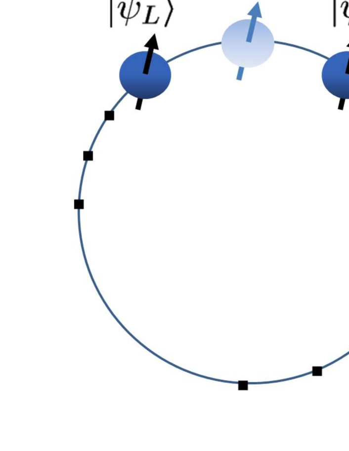
Figure 1: Schematic illustration of $2L$ qubits in a ring structure to measure globally applied fields with an uncertainty scaling as $1/T$ when we use separable states. Half of the qubits contain information about the target fields as a probe while the remaining half are used as ancillary qubits for the qubit teleportation. With a controlled phase gate and measurement feedforward operations, we can teleport a quantum state $|\psi\rangle$ from the original site to the right neighboring site Browne and Briegel (2006); Raussendorf and Briegel (2001). After the teleportation, the measured qubit becomes the new ancilla which we initialize into $|0\rangle$.

Scheme with separable states.– Now we explore a possibly more practical scheme with separable states, as shown in Fig. 1. We begin by preparing a probe state of $\bigotimes_{j=1}^{L}|+\rangle_{2j-1}$ located at the site $2j-1$ ($j=1,2,\cdots,L$). Then we let the state evolve for a time $\tau={t}/{n}$ and teleport the state of the probe qubit to the next site using the ancillary qubit. We repeat this step $(n-1)$ times before we finish by allowing our state to evolve for time $\tau=\frac{t}{n}$, and reading out the state by measuring $\hat{M}_{y}=\sum_{j=1}^{L}\hat{\sigma}_{y}^{(j)}$. We repeat these steps $N$ times during the measurement time $T$ where $N\simeq{T}/{t}$ is the repetition number. We can calculate the sensitivity for this scheme by substituting $M=1$ in Eq. 1. For an ideal QT, by setting $t=T$ and $p=0$, we obtain $\delta\omega_{n,T}\simeq{e^{1/4}}/{T\sqrt{L}}$ for $n=4\gamma^{2}T^{2}$, and so we can achieve $1/T$ scaling. For $n\geq\tilde{n}$, a correlated error may be induced due to the memory effect where $\tilde{n}=2L-1$ denotes the maximum number of teleportations without the qubit state being teleported back to the original site. Fortunately, since the typical environment has a finite correlation time $\tau_{c}$, such a correlation effect becomes negligible for a large number of qubits to satisfy $\tilde{n}\tau\gg\tau_{c}\Leftrightarrow L\gg\gamma^{2}T\tau_{c}$ (See the supplementary materials).

We now analyze how imperfect QT affects the performance of our sensing scheme. We can calculate the sensitivity by substituting $M=1$ and $p>0$ with Eq. 1. For a short time such as $T\ll{1}/{\sqrt{p}\gamma}$, the error due to QT is negligible, and so we obtain the same results as with perfect QT by setting $t=T$and $n=4\gamma^{2}T^{2}$, which allows us to achieve uncertainty scaling as $1/T$. We can minimize the uncertainty by setting $t_{\rm{opt}}={\sqrt{n}}/{2\gamma}$ as long as $T\gg t_{\rm{opt}}$ is satisfied. In such a case, $\delta\omega_{n,t_{\rm{opt}}}=\frac{\sqrt{2}e^{{1}/{4}}}{(1-p)^{n-1}}{\sqrt{\frac{\gamma}{\sqrt{n}TL}}}$, which for $n=1$ gives the standard Ramsey uncertainty $\delta\omega_{{\rm{R}}}=\frac{e^{{1}/{4}}\sqrt{\gamma}}{\sqrt{TL}}$ Huelga et al. (1997) where we replace $L$ with $2L$ (because the standard Ramsey scheme can utilize every qubit to probe the target fields without ancillary qubits). For $n\gg 1$. we can treat $n$ as a continuous variable, and we can analytically minimize the uncertainty as $\delta\omega_{\rm{opt}}\simeq 2\sqrt{\frac{e\sqrt{p}\gamma}{LT}}$ for ${1}/{16\gamma^{2}T^{2}}\ll p\ll 1$ where we choose $n_{\rm{opt}}=-{1}/{4\log(1-p)}\simeq{1}/{4p}$. The condition required for the error to be independent ($\tilde{n}\tau\geq\tau_{c}$) is written as $L\sqrt{p}/\gamma\gg\tau_{c}$, and is satisfied for a large $L$. In this case, we have a constant factor improvement over the standard Ramsey scheme for a longer $T$. In fact, as long as $p<0.0251$, our scheme is better than that standard Ramsey scheme (${\delta\omega_{{\rm{R}}}}/{\delta\omega_{{\rm{opt}}}}>1$). For $p=10^{-4}$, we obtain ${\delta\omega_{{\rm{R}}}}/{\delta\omega_{{\rm{opt}}}}\simeq 3.89$, So our sensor has an advantage with finite errors caused by the imperfect QT.

In conclusion, we have proposed a scheme designed to achieve sensitivity beyond the classical limit and to measure the amplitudes of globally applied fields. We have found that frequent implementations of quantum teleportation provide a suitable circumstance for sensing where the dephasing is suppressed while the information from the target fields is continuously accumulated. If perfect quantum teleportation is available, the uncertainty scales as $1/T$ with our scheme while any classical sensor shows the uncertainty scaled as $1/\sqrt{T}$. Moreover, even when quantum teleportation is moderately noisy, our protocol still realizes superior quantum enhancement to the standard Ramsey scheme. This work was supported by JSPS KAKENHI Grant No. 15K17732 and partly supported by MEXT KAKENHI Grant No. 15H05870. S.C.B. acknowledges support from the EPSRC NQIT Hub, Project No. EP/M013243/1.

Supplementary materials: This is a supplementary material of the paper titled “Quantum metrology beyond the classical limit under the effect of dephasing”.

Appendix A Error model

In the main text, we consider a specific noise model with which to calculate the sensitivity of our sensor, and we will explain how we can derive the model from the general expression. We consider the following general Hamiltonian to describe the dephasing.

$$H = H_{\rm{S}}+H_{\rm{I}}+H_{\rm{E}}$$

$$H_{\rm{S}} = \frac{\omega}{2}\sigma_{z}\otimes\openone_{\rm{E}}$$

$$H_{\rm{E}} = \openone_{\rm{S}}\otimes C$$

$H_{\rm{S}}$, $H_{\rm{I}}$, and $H_{\rm{E}}$ denote a system, an interaction, and an environmental Hamiltonian, respectively. As we describe in the main text, the perturbation theory allows us to solve the Schrodinger equation, and we obtain

$$\rho_{\rm{S}}(\tau)\simeq(1-\epsilon_{\tau})U_{\tau}\rho_{\rm{S}}(0)U_{\tau}^{\dagger}+\epsilon_{\tau}\hat{\sigma}_{z}U_{\tau}\rho_{\rm{S}}(0)U_{\tau}^{\dagger}\sigma_{z}$$ (3)

where $\epsilon_{\tau}=\lambda^{2}C_{0}\tau^{2}$ denotes an error rate for $\lambda^{2}C_{0}(\tau)^{2}\ll 1$ and $U_{\tau}=e^{-{i\omega\tau}\hat{\sigma}_{z}/2}$ denotes a unitary operator. We could approximate this expression by

$$\rho_{\rm{S}}(\tau)\simeq\frac{1+e^{-2\lambda^{2}C_{0}\tau^{2}}}{2}U_{\tau}\rho_{\rm{S}}(0)U_{\tau}^{\dagger}$$

$$+\frac{1-e^{-2\lambda^{2}C_{0}\tau^{2}}}{2}\hat{\sigma}_{z}U_{\tau}\rho_{\rm{S}}(0)U_{\tau}^{\dagger}\sigma_{z}$$ (4)

Actually, by performing a Taylor expansion such as $e^{-2\lambda^{2}C_{0}\tau^{2}}\simeq 1-2\lambda^{2}C_{0}\tau^{2}$ in Eq. (4), we can reproduce Eq. (3). By defining $\gamma^{2}=2\lambda^{2}C_{0}$, we obtain $\rho_{\rm{S}}(\tau)\simeq\frac{1+e^{-\gamma^{2}\tau^{2}}}{2}U_{\tau}\rho_{\rm{S}}(0)U_{\tau}^{\dagger}+\frac{1-e^{-\gamma^{2}\tau^{2}}}{2}\hat{\sigma}_{z}U_{\tau}\rho_{\rm{S}}(0)U_{\tau}^{\dagger}\sigma_{z}$. In the main text, we use this expression to quantify the effect of the dephasing during the operations in our sensing protocol. It is worth mentioning that, strictly speaking, the form of the Eq. 4 is the same as Eq. 3 only when $\gamma\tau\ll 1$. However, typical dephasing models Palma et al. (1996); De Lange et al. (2010); Kakuyanagi et al. (2007); Yoshihara et al. (2006) actually show the behavior described in Eq. (4) for an even longer time if the correlation time of the environment is much longer than the dephasing time, and this shows the validity of our assumption.

Appendix B Independent error accumulation

In our scheme, the environment interacts with teleported states of the qubit one after another. Here, we consider the decoherence dynamics for this case in more detail than in the main text. Specifically, we will show that, although the environment frequently interacts with the teleported states, the phase error on the qubit can be independent as long as a Born approximation is valid.

For simplicity, we consider just two sites for a Hamiltonian of the form $H=H_{\rm{S}}+H_{\rm{I}}+H_{\rm{E}}$ where $H_{\rm{S}}=\sum_{j=1}^{2}\frac{\omega}{2}\sigma^{(j)}_{z}$ ($H_{\rm{E}}=\sum_{j=1}^{2}\openone^{(j)}_{\rm{S}}\otimes C_{j}$) denotes the system (environmental) Hamiltonian, $H_{\rm{I}}=\sum_{j=1}^{2}\lambda\sigma^{(j)}_{z}\otimes B_{j}$ denotes an interaction between the system and the environment. $B_{j}$ and $C_{j}$ denote the environmental operators. In the interaction picture, we have $H_{\rm{I}}(t)=\lambda\sum_{j=1}^{2}\sigma^{(j)}_{z}\otimes\tilde{B}_{j}(t)$ where $\tilde{B}_{j}(t)=e^{iH_{\rm{E}}t}B_{j}e^{-iH_{\rm{E}}t}$. The initial state is given as $\rho(0)=\rho_{\rm{S}}(0)\otimes\rho_{\rm{S}}(0)\otimes\rho^{(1)}_{\rm{E}}\otimes\rho^{(2)}_{\rm{E}}$. We also assume that $\rho^{(j)}_{\rm{E}}$ is in thermal equilibrium such that $[\rho^{(j)}_{\rm{E}},H_{\rm{E}}]=0$ and our noise is non-biased such that ${\rm{Tr}}[\rho^{(j)}_{\rm{E}}B_{j}]=0$. We consider the following case. After the environment interacts with the system qubit at each site for a time $0\leq t\leq\tau$, we perform a quantum teleportation to send the state at site 1 to site 2 (while the state at site 2 is teleported to another site), and the environment interacts with the new state at each site for a time $\tau\leq t\leq 2\tau$. To describe the interaction between the system and environment before the quantum teleportation, we use the Schrodinger equation

$$\frac{d\rho_{I}(t)}{dt}=-i[H_{I}(t),\rho_{I}(t)].$$ (5)

By integrating this, we obtain

$$\rho_{I}(t) = \rho(0)-i\int_{0}^{t}dt^{\prime}[H_{I}(t^{\prime}),\rho(0)]$$

$$- i\int_{0}^{t}\int_{0}^{t^{\prime}}dt^{\prime}dt^{\prime\prime}[H_{I}(t^{\prime}),[H_{I}(t^{\prime\prime}),\rho(t^{\prime\prime})]]$$

Since there are no interactions between site 1 and site 2, we consider that the state at site 1 is separable from the state at the site 2.

$$\rho^{(j)}_{\rm{I}}(\tau)\simeq\rho^{(j)}(0)-i\lambda\int_{0}^{\tau}dt^{\prime}\lambda[\sigma^{(j)}_{z}\otimes\tilde{B}_{j}(t^{\prime}),\rho(0)]$$

$$-\lambda^{2}\int_{0}^{\tau}\int_{0}^{t^{\prime}}dt^{\prime}dt^{\prime\prime}[\sigma^{(j)}_{z}\otimes\tilde{B}_{j}(t^{\prime}),[\sigma^{(j)}_{z}\otimes\tilde{B}_{j}(t^{\prime\prime}),\rho(0)]]$$

for $j=1,2$ where we use a second order perturbation expansion in $\lambda$. We use the Born approximation $\rho^{(j)}_{\rm{I}}(\tau)\simeq\rho^{(j)}_{\rm{S}}(\tau)\otimes\rho^{(j)}_{\rm{E}}$ Hornberger (2009). This means that, since the environment has a large degree of freedom, the correlation between the system and the environment is negligible. In fact, it is known that the Born approximation becomes more accurate as the size of the bath is increased Hasegawa (2011); Carcaterra and Akay (2011). By tracing out the environment, we obtain

$$\rho^{(j)}_{\rm{S}}(\tau) \simeq \rho_{\rm{S}}(0)$$

$$-\lambda^{2}\int_{0}^{\tau}\int_{0}^{t^{\prime}}dt^{\prime}dt^{\prime\prime}C^{(j)}_{t^{\prime}-t^{\prime\prime}}\left[\hat{\sigma}^{(j)}_{z},\left[\hat{\sigma}^{(j)}_{z},\rho_{\rm{S}}(0)\right]\right]$$

for $j=1,2$ where $C^{(j)}_{t^{\prime}-t^{\prime\prime}}\equiv\frac{1}{2}{\rm{Tr}}[(\tilde{B}_{j}(t^{\prime})\tilde{B}_{j}(t^{\prime\prime})+\tilde{B}_{j}(t^{\prime\prime})\tilde{B}_{j}(t^{\prime}))\rho^{(j)}_{\rm{E}}]$ denotes the correlation function of the environment at the site $j$. It is worth mentioning that the correlation function does not depend on the state of the system but depends on the properties of the environment. By performing a quantum teleportation to send the state at site 1 to site 2 (while the state at site 2 is teleported to another site), we obtain

$$\rho^{\prime(2)}_{\rm{S}}(\tau) \simeq \rho_{\rm{S}}(0)$$

$$-\lambda^{2}\int_{0}^{\tau}\int_{0}^{t^{\prime}}dt^{\prime}dt^{\prime\prime}C^{(1)}_{t^{\prime}-t^{\prime\prime}}\left[\hat{\sigma}^{(2)}_{z},\left[\hat{\sigma}^{(2)}_{z},\rho_{\rm{S}}(0)\right]\right]$$

at site 2. By allowing this state to interact with the environment for a time $\tau\leq t\leq 2\tau$, we obtain

$$\rho^{\prime(2)}_{\rm{I}}(2\tau)\simeq\rho_{\rm{I}}^{\prime(2)}(\tau)-i\lambda\int_{\tau}^{2\tau}dt^{\prime}\lambda[\sigma^{(2)}_{z}\otimes\tilde{B}_{2}(t^{\prime}),\rho^{\prime(2)}_{\rm{I}}(\tau)]$$

$$-\lambda^{2}\int_{\tau}^{2\tau}\int_{\tau}^{t^{\prime}}dt^{\prime}dt^{\prime\prime}[\sigma^{(2)}_{z}\otimes\tilde{B}_{2}(t^{\prime}),[\sigma^{(2)}_{z}\otimes\tilde{B}_{2}(t^{\prime\prime}),\rho_{\rm{I}}^{\prime(2)}(\tau)]]$$

where we consider $\rho_{\rm{I}}^{\prime(2)}(\tau)=\rho^{\prime(2)}_{\rm{S}}(\tau)\otimes\rho_{\rm{E}}^{(2)}$ as the initial state. By tracing out the environment, we obtain

$$\rho^{\prime(2)}_{\rm{S}}(2\tau)\simeq\rho^{\prime(2)}_{\rm{S}}(\tau)$$

$$-\lambda^{2}\int_{\tau}^{2\tau}\int_{\tau}^{t^{\prime}}dt^{\prime}dt^{\prime\prime}C^{(2)}_{t^{\prime}-t^{\prime\prime}}\left[\hat{\sigma}^{(2)}_{z},\left[\hat{\sigma}^{(2)}_{z},\rho^{\prime(2)}_{\rm{S}}(\tau)\right]\right]$$

where we use a Born approximation such as $\rho_{\rm{I}}^{\prime(2)}(2\tau)\simeq\rho^{\prime(2)}_{\rm{S}}(2\tau)\otimes\rho_{\rm{E}}^{(2)}$. By considering up to the second order term of $\lambda$, we obtain

$$\rho^{\prime(2)}_{\rm{S}}(2\tau)\simeq\rho_{\rm{S}}(0)$$

$$- \lambda^{2}\int_{0}^{\tau}\int_{0}^{t^{\prime}}dt^{\prime}dt^{\prime\prime}C^{(1)}_{t^{\prime}-t^{\prime\prime}}\left[\hat{\sigma}^{(2)}_{z},\left[\hat{\sigma}^{(2)}_{z},\rho_{\rm{S}}(0)\right]\right]$$

$$- \lambda^{2}\int_{\tau}^{2\tau}\int_{\tau}^{t^{\prime}}dt^{\prime}dt^{\prime\prime}C^{(2)}_{t^{\prime}-t^{\prime\prime}}\left[\hat{\sigma}^{(2)}_{z},\left[\hat{\sigma}^{(2)}_{z},\rho_{\rm{S}}(0)\right]\right].$$

Since $C^{(2)}_{t^{\prime}-t^{\prime\prime}}$ does not depend on the absolute value of $t^{\prime}$ (or $t^{\prime\prime}$) but depends on the time difference $t^{\prime}-t^{\prime\prime}$, we obtain

$$\rho^{\prime(2)}_{\rm{S}}(2\tau)\simeq\rho_{\rm{S}}(0)$$

$$- \lambda^{2}\int_{0}^{\tau}\int_{0}^{t^{\prime}}dt^{\prime}dt^{\prime\prime}C^{(1)}_{t^{\prime}-t^{\prime\prime}}\left[\hat{\sigma}^{(2)}_{z},\left[\hat{\sigma}^{(2)}_{z},\rho_{\rm{S}}(0)\right]\right]$$

$$- \lambda^{2}\int_{0}^{\tau}\int_{0}^{t^{\prime}}dt^{\prime}dt^{\prime\prime}C^{(2)}_{t^{\prime}-t^{\prime\prime}}\left[\hat{\sigma}^{(2)}_{z},\left[\hat{\sigma}^{(2)}_{z},\rho_{\rm{S}}(0)\right]\right].$$

So the interaction between the system and the environment at site 1 for a time $0\leq t\leq\tau$ does not induce a correlation in the decoherence dynamics between the system and environment at site 2. (There is no effect such as an accelerated or deaccelerated noise accumulation of the dephasing at site 2 due to past decoherence at site 1.) So the $\hat{\sigma}_{z}$ error caused by the environment at site $2$ acts on the qubit independently of the $\hat{\sigma}_{z}$ error caused by the environment at site $1$.

Although we consider the dynamics at sites $1$ and $2$ above, we can easily generalize this to $n$ sites. By repeating the above calculations, we obtain

$$\rho^{\prime(n)}_{\rm{S}}(n\tau)\simeq\rho_{\rm{S}}(0)$$

$$- \sum_{j=1}^{n}\lambda^{2}\int_{0}^{\tau}\int_{0}^{t^{\prime}}dt^{\prime}dt^{\prime\prime}C^{(j)}_{t^{\prime}-t^{\prime\prime}}\left[\hat{\sigma}^{(n)}_{z},\left[\hat{\sigma}^{(n)}_{z},\rho_{\rm{S}}(0)\right]\right]$$

at site $n$ after $n-1$ teleportation where the $\hat{\sigma}_{z}$ error accumulates independently at each site, and this is consistent with the calculations in the main text.

Appendix C Effect of a finite number of the qubits

In the main text, we did not mention the case where the qubits are teleported back to the original sites whose environment the qubit initially interacted with. If qubits have the chance to interact with the environment with which they previously interacted, this may induce a correlated error on the qubit. However, we will show that we can still avoid the correlated error as long as there are a large number of the qubits, which is a common assumption in the field of quantum metrology..

For simplicity, we consider just a single site for a Hamiltonian of the form $H=H_{\rm{S}}+H_{\rm{I}}+H_{\rm{E}}$ where $H_{\rm{S}}=\frac{\omega}{2}\sigma_{z}$ ($H_{\rm{E}}=\openone_{\rm{S}}\otimes C_{j}$) denotes the system (environmental) Hamiltonian, and $H_{\rm{I}}=\lambda f(t)\sigma_{z}\otimes B_{j}$ denotes an interaction between the system and the environment. $B$ and $C$ denote environmental operators. We define $f(t)$ as follows

$$f(t)=\begin{cases}1&(0\leq t\leq\tau)\\ 1&((m-1)\tau\leq t\leq m\tau)\\ 0&({\rm{otherwise}})\end{cases}$$

where $m$ denotes a natural number. This means that, after the qubit interacts with the environment for a time $(0\leq t\leq\tau)$, the qubit is decoupled from the environment for a time $\tau<t<n\tau$, and the qubit interacts with the same environment again for a time $m\tau\leq t\leq(m+1)\tau$. From this calculation, we can estimate the way in which the correlated error will be induced by multiple interactions with the same environment in our scheme. Using a similar calculation to that used in the previous section, we obtain

$$\rho_{\rm{S}}(n\tau)\simeq\rho_{\rm{S}}(0)$$

$$-\lambda^{2}\int_{0}^{m\tau}\int_{0}^{t^{\prime}}dt^{\prime}dt^{\prime\prime}f(t^{\prime})f(t^{\prime\prime})C_{t^{\prime}-t^{\prime\prime}}\left[\hat{\sigma}_{z},\left[\hat{\sigma}_{z},\rho_{\rm{S}}(0)\right]\right]$$

where we solve the Schrodinger equation for a time $0\leq t\leq m\tau$. We obtain

$$\rho_{\rm{S}}(m\tau)-\rho_{\rm{S}}(0)\simeq$$

$$-\lambda^{2}(\int_{0}^{\tau}+\int_{(m-1)\tau}^{m\tau})dt^{\prime}\int_{0}^{t^{\prime}}dt^{\prime\prime}f(t^{\prime})f(t^{\prime\prime})C_{t^{\prime}-t^{\prime\prime}}\left[\hat{\sigma}_{z},\left[\hat{\sigma}_{z},\rho_{\rm{S}}(0)\right]\right]$$

$$=-\lambda^{2}\int_{0}^{\tau}dt^{\prime}\int_{0}^{t^{\prime}}dt^{\prime\prime}f(t^{\prime})f(t^{\prime\prime})C_{t^{\prime}-t^{\prime\prime}}\left[\hat{\sigma}_{z},\left[\hat{\sigma}_{z},\rho_{\rm{S}}(0)\right]\right]$$

$$-\lambda^{2}\int_{(m-1)\tau}^{m\tau}dt^{\prime}\int_{0}^{t^{\prime}}dt^{\prime\prime}f(t^{\prime})f(t^{\prime\prime})C_{t^{\prime}-t^{\prime\prime}}\left[\hat{\sigma}_{z},\left[\hat{\sigma}_{z},\rho_{\rm{S}}(0)\right]\right]$$

$$=-\lambda^{2}\int_{0}^{\tau}dt^{\prime}\int_{0}^{t^{\prime}}dt^{\prime\prime}C_{t^{\prime}-t^{\prime\prime}}\left[\hat{\sigma}_{z},\left[\hat{\sigma}_{z},\rho_{\rm{S}}(0)\right]\right]$$

$$-\lambda^{2}\int_{(m-1)\tau}^{m\tau}dt^{\prime}\int_{0}^{\tau}dt^{\prime\prime}C_{t^{\prime}-t^{\prime\prime}}\left[\hat{\sigma}_{z},\left[\hat{\sigma}_{z},\rho_{\rm{S}}(0)\right]\right]$$

$$-\lambda^{2}\int_{(m-1)\tau}^{m\tau}dt^{\prime}\int_{(n-1)\tau}^{t^{\prime}}dt^{\prime\prime}C_{t^{\prime}-t^{\prime\prime}}\left[\hat{\sigma}_{z},\left[\hat{\sigma}_{z},\rho_{\rm{S}}(0)\right]\right]$$

The term $\lambda^{2}\int_{(m-1)\tau}^{m\tau}dt^{\prime}\int_{0}^{\tau}dt^{\prime\prime}C_{t^{\prime}-t^{\prime\prime}}\left[\hat{\sigma}_{z},\left[\hat{\sigma}_{z},\rho_{\rm{S}}(0)\right]\right]$ represents the correlated effect of an environment that has a memory of the first interaction with the qubit when it has the second interaction with the qubit. It is worth mentioning that a typical environment has a finite correlation time $\tau_{c}$ Romach et al. (2015); De Lange et al. (2010); Kondo et al. (2016); Wilhelm et al. (2007); Hall et al. (2014); Koppens et al. (2007), and so the correlation function for a longer time scale than the correlation time such as $C_{t^{\prime}-t^{\prime\prime}}\simeq 0$ for $|t^{\prime}-t^{\prime\prime}|\gg\tau_{c}$ has a negligible effect. This means that, if we have $m\tau\gg\tau_{c}$, we obtain

$$\rho_{\rm{S}}(m\tau)\simeq\rho_{\rm{S}}(0)$$

$$-\lambda^{2}\int_{0}^{\tau}dt^{\prime}\int_{0}^{t^{\prime}}dt^{\prime\prime}C_{t^{\prime}-t^{\prime\prime}}\left[\hat{\sigma}_{z},\left[\hat{\sigma}_{z},\rho_{\rm{S}}(0)\right]\right]$$

$$-\lambda^{2}\int_{(m-1)\tau}^{m\tau}dt^{\prime}\int_{(m-1)\tau}^{t^{\prime}}dt^{\prime\prime}C_{t^{\prime}-t^{\prime\prime}}\left[\hat{\sigma}_{z},\left[\hat{\sigma}_{z},\rho_{\rm{S}}(0)\right]\right]$$

$$\simeq \rho_{\rm{S}}(0)-2\lambda^{2}\int_{0}^{\tau}dt^{\prime}\int_{0}^{t^{\prime}}dt^{\prime\prime}C_{t^{\prime}-t^{\prime\prime}}\left[\hat{\sigma}_{z},\left[\hat{\sigma}_{z},\rho_{\rm{S}}(0)\right]\right],$$

and the correlated effect of the environment becomes negligible. So the decoherence acts on the qubit independently as long as we have $m\tau\gg\tau_{c}$. We define $\tilde{n}$ as the maximum teleportation number without the qubit state being teleported back to the original site. (For example, in the teleportation-based scheme with a ring structure described in the main text for separable states, we have $\tilde{n}=2L-1$.) We can substitute $m=\tilde{n}$, and the condition needed for the error to be independent is $\tilde{n}\tau\gg\tau_{c}$.

Appendix D High frequency noise

In the main text, we consider the effect of dephasing as decoherence. There are of course other sources of decoherence that cannot be suppressed by the quantum teleportation (QT) protocol, and we consider such an effect. If our quantum systems are affected by high-frequency noise with a short correlation time, the decay is not quadratic in nature but more exponential-like. Energy relaxation in a high temperature environment is known to induce such noise Gardiner and Zoller (2004). Consider the situation in which an initial state $|+\rangle_{j}$ evolves under the effect of both low-frequency dephasing and high-frequency noise for a time $\tau$. In such a case $\rho^{(j)}_{\rm{S}}(\tau)=\frac{1}{2}(\openone_{j}+|1\rangle_{j}\langle 0|e^{-i\omega\tau-\gamma^{2}\tau^{2}-\Gamma\tau}+|0\rangle_{j}\langle 1|e^{i\omega\tau-\gamma^{2}\tau^{2}-\Gamma\tau})$ where $\Gamma$ denotes the decay rate associated with the high-frequency noise ($\Gamma=0$ gives the same noise model as the one we used previously). It is then straightforward to calculate the uncertainty of the estimation under the effect of this noise with imperfect QT as $\delta\omega_{n,t}=\frac{e^{\Gamma t+{\gamma^{2}t^{2}}/{n}}}{(1-p)^{n-1}}\frac{1}{\sqrt{TtL}}$. Choosing $t_{\rm{opt}}=\frac{-\sqrt{n}m+\sqrt{nm^{2}+4}}{4(\gamma/\sqrt{n})}$ (where $m={\Gamma}/{\gamma}$), we minimize this with respect to time as

$$\delta\omega_{n,t_{\rm{opt}}}=\frac{2\sqrt{\gamma}e^{\frac{1}{4}+\frac{-nm^{2}+m\sqrt{n(nm^{2}+4)}}{8}}}{(1-p)^{n-1}\sqrt{(-nm+\sqrt{n(nm^{2}+4)})LT}}.$$

The uncertainty with $n$ can be numerically minimized as $\delta\omega_{\rm{opt}}=\min_{n}\delta\omega_{n,t_{\rm{opt}}}$. In Fig. 2, we plot $\delta\omega_{\rm{R}}/\delta\omega_{\rm{opt}}$ versus $p$ and ${\Gamma}/{\gamma}$ where $\delta\omega_{\rm{R}}$ is the uncertainty for the standard Ramsey scheme. Our plots shows that our scheme performs better than the standard Ramsey scheme for $\Gamma/\gamma<0.130$ and $p<0.0123$ .

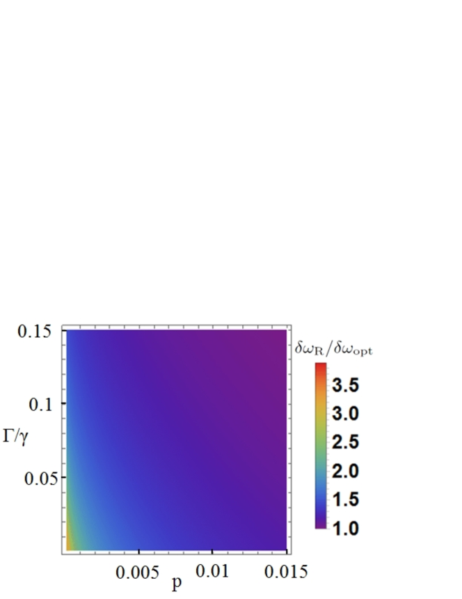
Figure 2: Performance of our teleportation based scheme against the standard Ramsey scheme. We plot $\delta\omega_{\rm{R}}/\delta\omega_{\rm{opt}}$ against $\frac{\Gamma}{\gamma}$ and $p$. Our scheme performs better than the standard Ramsey scheme for $\Gamma/\gamma<0.130$ and $p<0.0123$ .

Appendix E Implementation of quantum metrology beyond the classical limit under the effect of dephasing with global control

In the scheme described in the main text, we suggest the use of quantum teleportation to suppress dephasing. To implement this scheme, the quantum teleportation. which involves projective measurements and feedback operations, should be performed in a much shorter time than the correlation time of the environment. Also, the individual controllability of the qubit is needed to implement quantum teleportation for every qubit. In the state of the art technology, a gate control with a fidelity of more than 99% has been realized for some systems such as superconducting qubits and ion trap systems Barends et al. (2014); Ballance et al. (2016); Blume-Kohout et al. (2017). Moreover, many groups aim to realize a scalable quantum computer, and a quantum supremacy with 50 qubits could be demonstrated in the near future Neill et al. (2017); Popkin (2016). Such a development of quantum technology toward the demonstration of quantum computation also supports the realization of our teleportation-based scheme. So our scheme is within the reach of such a future technology.

However, it is still worth discussing how to realize our scheme with simpler technology and thus improve the practicality. In this section, we suggest an alternative scheme for this purpose, which is useful for our separable states scheme. Here, we use a direct interaction between the qubits. We show that a simple modulation of the Hamiltonian can transfer the states to suppress the dephasing where neither individual addressability nor rapid measurement is required.

Figure 3: Schematic illustration of our SWAP-based sensing where we arrange $2L$ qubits in a ring structure. Similar to the teleportation-based scheme described in the main text, half of the qubits contain an information of the target fields as a probe while the remaining half are used as an ancilla qubits kept in a ground state. We assume a flip-flop type interaction between nearest neighbor qubits. For the half of the qubits, the frequency is fixed at $\omega_{A}$ or $\omega_{B}$ where $\omega_{A}$ is well detuned from $\omega_{B}$, while a frequency of the other half of the qubits is tunable. If we set the tunable frequency as $\omega_{A}$ or $\omega_{B}$, the flip-flop interaction becomes effective, and so we can perform a SWAP gate between the probe qubits and ancillary qubits by a time evolution with the Hamiltonian. On the other hand, we set the tunable frequency as $\omega_{C}$ where $\omega_{C}$ is well detuned from both $\omega_{A}$ and $\omega_{B}$, the flip-flop interaction is significantly suppressed by the detuning. In this configuration, the modulation of the frequency can transfer the state of the probe qubits to the clock wise direction.

The main difference from the scheme described in the main text is that, instead of quantum teleportation, we use a SWAP operation between the probe qubit at a site and an ancillary qubit at the neighboring site on the right, as shown in Fig. 3. First, we arrange qubits in a ring structure, and we prepare a state of $\bigotimes_{j=1}^{L}|+\rangle_{2j-1}$ located at site $2j-1$ ($j=1,2,\cdots,L$) for probe qubits, while we prepare $\bigotimes_{j=1}^{L}|0\rangle_{2j}$ located at site $2j$ ($j=1,2,\cdots,L$) for the ancillary qubits. For simplicity, we assume that $L$ is an even number. Second, we then let the state evolve for a time $\tau={t}/{n}$ and then perform a SWAP gate between the probe qubit and the ancillary qubit at the neighboring site on the right (we assume that our gate operations are much faster than $\tau$). Third, we repeat the second step $(n-1)$ times while in the fourth step we allow this state to evolve for a time $\tau=\frac{t}{n}$, and readout the state by measuring $\hat{M}_{y}=\sum_{j=1}^{L}\hat{\sigma}_{y}^{(j)}$. Finally, we repeat these steps $N$ times during the measurement time $T$ where $N\simeq{T}/{t}$ is the repetition number.

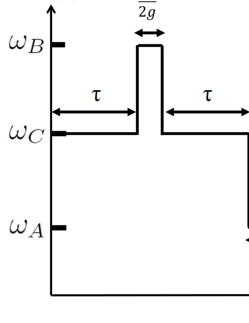
Figure 4: Modulation of the frequency of the qubit to implement our SWAP-based scheme. The qubit frequency is either $\omega_{A}$, $\omega_{B}$, or $\omega_{C}$ where these frequencies are well detuned from each other. Also, $g$ denotes the coupling strength between the qubits and $\tau=\frac{t}{n}$ denotes an interaction time with the fields. Here, we assume $\tau\gg\frac{1}{g}$. The modulation of the frequency with a flip-flop type interaction provides us with a way to transfer the state of the probe qubit to the clock wise direction as shown in the Fig. 3.

Importantly, we can implement the SWAP gate by using a direct interaction between the qubits, and we can turn on/off the interaction by modulating the frequency of the qubit. We consider the following flip-flop type Hamiltonian.

$$H=\sum_{j=1}^{2L}\frac{\omega+\omega_{j}}{2}\hat{\sigma}_{z}^{(j)}+g(\hat{\sigma}_{+}^{(j)}\hat{\sigma}_{-}^{(j+1)}+\hat{\sigma}_{-}^{(j)}\hat{\sigma}_{+}^{(j+1)})$$ (8)

where $\omega_{j}$ denotes the frequency of the qubit at the $j$ th site. We also consider a periodic condition such as $\hat{\sigma}_{\pm}^{(2L+1)}=\hat{\sigma}_{\pm}^{(1)}$. We set the frequency of the qubit as

$$\omega_{j}=\begin{cases}\tilde{\omega}(t)&j\equiv 1\ ({\rm{mod}}\ 4)\\ \omega_{A}&j\equiv 2\ ({\rm{mod}}\ 4)\\ \tilde{\omega}^{\prime}(t)&j\equiv 3\ ({\rm{mod}}\ 4)\\ \omega_{B}&j\equiv 4\ ({\rm{mod}}\ 4)\end{cases}$$

where $\tilde{\omega}(t)$ and $\tilde{\omega}^{\prime}(t)$ denote a tunable time-dependent frequency, as shown in Fig. 4. In addition, we assume a large detuning between $\omega_{A}$ and $\omega_{B}$. Here, we focus on two adjacent qubits, and the Hamiltonian is given as

$$H^{(k,k+1)} = H^{(k,k+1)}_{0}+H^{(k,k+1)}_{1}$$

$$H^{(k,k+1)}_{0} = \frac{\omega+\tilde{\omega}_{k}}{2}\hat{\sigma}_{z}^{(k)}+\frac{\omega+\tilde{\omega}_{k+1}}{2}\hat{\sigma}_{z}^{(k+1)}$$

$$H^{(k,k+1)}_{1} = g(\hat{\sigma}_{+}^{(k)}\hat{\sigma}_{-}^{(k+1)}+\hat{\sigma}_{-}^{(k)}\hat{\sigma}_{+}^{(k+1)})$$ (9)

where one of the qubits is a probe and the other qubit is an ancilla. In an interaction picture, we have

$$H^{(k,k+1)}_{I}=\frac{\tilde{\omega}_{k}-\tilde{\omega}_{k+1}}{2}\hat{\sigma}_{z}^{(1)}+g(\hat{\sigma}_{+}^{(k)}\hat{\sigma}_{-}^{(k+1)}+\hat{\sigma}_{-}^{(k)}\hat{\sigma}_{+}^{(k+1)})$$

If we have large detuning between these two qubits such as $|\tilde{\omega}_{k}-\tilde{\omega}_{k+1}|\gg g$, we obtain

$$H_{I}^{(k,k+1)}\simeq\frac{\tilde{\omega}_{k}-\tilde{\omega}_{k+1}}{2}\hat{\sigma}_{z}^{(k)}$$ (10)

where the coupling is effectively turned off. On the other hand, if we have a resonant condition such as $\tilde{\omega}_{k}=\tilde{\omega}_{k+1}$

$$H_{I}^{(k,k+1)}=g(\hat{\sigma}_{+}^{(k)}\hat{\sigma}_{-}^{(k+1)}+\hat{\sigma}_{-}^{(k)}\hat{\sigma}_{+}^{(k+1)})$$ (11)

In this case, the interaction is turned on, and a unitary operation $U=e^{iH^{(k,k+1)}\frac{\pi}{2g}}$ provides us with a SWAP gate between the probe qubit and ancillary qubit up to local operations. This means that, if we set $\tilde{\omega}(t)=\omega_{A}$ ($\tilde{\omega}(t)=\omega_{B}$), a probe qubit and ancillary qubit with a frequency of $\omega_{A}$ ($\omega_{B}$) start the interaction under a resonant condition, while these qubits do not interact with the other qubits with a frequency of $\omega_{B}$ ($\omega_{A}$). On the other hand, if we set $\tilde{\omega}(t)=\omega_{C}$ where $|\omega_{A}-\omega_{C}|\gg g$ and $|\omega_{B}-\omega_{C}|\gg g$, the qubit does not interact with any other qubits due to the large detuning. Therefore, the simple modulation of the qubit frequency (described in Fig. 4) realizes qubit motion in the same manner as that described in the main text with quantum teleportation. This is much more practical than the teleportation-based scheme, because neither individual addressability nor a rapid measurement is required for the SWAP-based scheme.

References

Budker and Romalis (2007)
D. Budker and
M. Romalis,
Nature Physics 3,
227 (2007).
Balasubramanian and et
al (2008)
G. Balasubramanian
and et al,
Nature 455,
648 (2008).
Maze and et al (2008)
J. Maze and
et al, Nature
455, 644 (2008),
ISSN 0028-0836.
Degen et al. (2016)
C. Degen,
F. Reinhard, and
P. Cappellaro,
arXiv preprint arXiv:1611.02427 (2016).
Simon (1999)
J. Simon,
Advances in Physics 48,
449 (1999).
Chang et al. (1992)
A. Chang,
H. Hallen,
L. Harriott,
H. Hess,
H. Kao,
J. Kwo,
R. Miller,
R. Wolfe,
J. Van der Ziel,
and T. Chang,
Applied physics letters 61,
1974 (1992).
Poggio and Degen (2010)
M. Poggio and
C. Degen,
Nanotechnology 21,
342001 (2010).
Huelga et al. (1997)
S. Huelga,
C. Macchiavello,
T. Pellizzari,
A. Ekert,
M. Plenio, and
J. Cirac,
Phys. Rev. Lett. 79,
3865 (1997).
Said et al. (2011)
R. Said,
D. Berry, and
J. Twamley,
Physical Review B 83,
125410 (2011).
Higgins et al. (2007)
B. L. Higgins,
D. W. Berry,
S. D. Bartlett,
H. M. Wiseman,
and G. J. Pryde,
Nature 450,
393 (2007).
Waldherr et al. (2012)
G. Waldherr,
J. Beck,
P. Neumann,
R. Said,
M. Nitsche,
M. Markham,
D. Twitchen,
J. Twamley,
F. Jelezko, and
J. Wrachtrup,
Nature nanotechnology 7,
105 (2012).
Demkowicz-Dobrzanski
et al. (2012)
R. Demkowicz-Dobrzanski,
J. Kolodynski,
and M. Guta,
Nature Communications 3
(2012).
Gottesman (2009)
D. Gottesman,
Proceedings of Symposia in Applied Mathematics
68, 13 (2009).
Viola et al. (1999)
L. Viola,
E. Knill, and
S. Lloyd,
Phys. Rev. Lett. 82,
2417 (1999).
Taylor et al. (2008)
J. Taylor,
P. Cappellaro,
L. Childress,
L. Jiang,
D. Budker,
P. Hemmer,
A. Yacoby,
R. Walsworth,
and M. Lukin,
Nature Physics 4,
810 (2008).
De Lange et al. (2011)
G. De Lange,
D. Ristè,
V. Dobrovitski,
and R. Hanson,
Phys. Rev. Lett. 106,
080802 (2011).
Dür et al. (2014)
W. Dür,
M. Skotiniotis,
F. Froewis, and
B. Kraus,
Phys. Rev. Lett. 112,
080801 (2014).
Herrera-Martí
et al. (2015)
D. A. Herrera-Martí,
T. Gefen,
D. Aharonov,
N. Katz, and
A. Retzker,
Phys. Rev. Lett. 115,
200501 (2015).
Arrad et al. (2014)
G. Arrad,
Y. Vinkler,
D. Aharonov, and
A. Retzker,
Phys. Rev. Lett. 112,
150801 (2014).
Kessler et al. (2014)
E. M. Kessler,
I. Lovchinsky,
A. O. Sushkov,
and M. D. Lukin,
Phys. Rev. Lett. 112,
150802 (2014).
Cohen et al. (2016)
L. Cohen,
Y. Pilnyak,
D. Istrati,
A. Retzker, and
H. Eisenberg,
Phys. Rev. A 94,
012324 (2016).
Unden et al. (2016)
T. Unden,
P. Balasubramanian,
D. Louzon,
Y. Vinkler,
M. B. Plenio,
M. Markham,
D. Twitchen,
A. Stacey,
I. Lovchinsky,
A. O. Sushkov,
et al., Phys. Rev. Lett.
116, 230502
(2016).
Sisi and et al (2017)
Z. Sisi and
et al, arXiv
preprint arXiv:1706.02445 (2017).
Schmitt and et al (2017)
S. Schmitt and
et al, Science
356, 832 (2017).
Boss et al. (2017)
J. Boss,
K. Cujia,
J. Zopes, and
C. Degen,
Science 356,
837 (2017).
Misra and Sudarshan (1977)
B. Misra and
E. G. Sudarshan,
Journal of Mathematical Physics
18, 756 (1977).
Itano et al. (1990)
W. Itano,
D. Heinzen,
J. Bollinger,
and D. Wineland,
Phys. Rev. A 41,
2295 (1990).
Facchi et al. (2001)
P. Facchi,
H. Nakazato, and
S. Pascazio,
Phys. Rev. Lett. 86,
2699 (2001).
Nakazato et al. (1996)
H. Nakazato,
M. Namiki, and
S. Pascazio,
Int. J. Mod. B 10,
247 (1996).
Raussendorf and Briegel (2001)
R. Raussendorf and
H. Briegel,
Phys. Rev. Lett. 86,
5188 (2001).
Barjaktarevic et al. (2005)
J. Barjaktarevic,
R. McKenzie,
J. Links, and
G. Milburn,
Phys. Rev. Lett. 95,
230501 (2005).
Silva et al. (2007)
M. Silva,
V. Danos,
E. Kashefi, and
H. Ollivier,
New Journal of Physics 9,
192 (2007).
Olmschenk et al. (2009)
S. Olmschenk,
D. Matsukevich,
P. Maunz,
D. Hayes,
L.-M. Duan, and
C. Monroe,
Science 323,
486 (2009).
Baur et al. (2012)
M. Baur,
A. Fedorov,
L. Steffen,
S. Filipp,
M. Da Silva, and
A. Wallraff,
Phys. Rev. Lett. 108,
040502 (2012).
Averin et al. (2016)
D. Averin,
K. Xu,
Y. Zhong,
C. Song,
H. Wang, and
S. Han,
Phys. Rev. Lett. 116,
010501 (2016).
Hornberger (2009)
K. Hornberger, in
Entanglement and Decoherence
(Springer, 2009), pp.
221–276.
De Lange et al. (2010)
G. De Lange,
Z. Wang,
D. Riste,
V. Dobrovitski,
and R. Hanson,
Science 330,
60 (2010).
Yoshihara et al. (2006)
F. Yoshihara,
K. Harrabi,
A. Niskanen, and
Y. Nakamura,
Phys. Rev. Lett. 97,
167001 (2006).
Kakuyanagi et al. (2007)
K. Kakuyanagi,
T. Meno,
S. Saito,
H. Nakano,
K. Semba,
H. Takayanagi,
F. Deppe, and
A. Shnirman,
Phys. Rev. Lett. 98,
047004 (2007).
Kondo et al. (2016)
Y. Kondo,
Y. Matsuzaki,
K. Matsushima,
and J. G.
Filgueiras, New Journal of Physics
18, 013033
(2016).
Palma et al. (1996)
G. M. Palma,
K. A. Suominen,
and A. K. Ekert,
Proc. R. Soc. London. Ser.A
452, 567 (1996).
Browne and Briegel (2006)
D. E. Browne and
H. J. Briegel
(2006), quant-ph/0603226.
Schaffry et al. (2010)
M. Schaffry,
E. M. Gauger,
J. J. Morton,
J. Fitzsimons,
S. C. Benjamin,
and B. W.
Lovett, Physical Review A
82, 042114
(2010).
Jones et al. (2009)
J. A. Jones,
S. D. Karlen,
J. Fitzsimons,
A. Ardavan,
S. C. Benjamin,
G. A. D. Briggs,
and J. J.
Morton, Science
324, 1166 (2009).
Matsuzaki et al. (2011)
Y. Matsuzaki,
S. Benjamin, and
J. Fitzsimons,
Phys. Rev. A 84,
012103 (2011).
Chin et al. (2012)
A. W. Chin,
S. F. Huelga,
and M. B.
Plenio, Phys. Rev. Lett.
109, 233601
(2012).
Shaji and Caves (2007)
A. Shaji and
C. M. Caves,
Physical Review A 76,
032111 (2007).
Bohmann et al. (2015)
M. Bohmann,
J. Sperling, and
W. Vogel,
Physical Review A 91,
042332 (2015).
Hornberger (2009)
K. Hornberger, in
Entanglement and Decoherence
(Springer, 2009), pp.
221–276.
Hasegawa (2011)
H. Hasegawa,
Physical Review E 83,
021104 (2011).
Carcaterra and Akay (2011)
A. Carcaterra and
A. Akay,
Physical Review E 84,
011121 (2011).
Romach et al. (2015)
Y. Romach,
C. Müller,
T. Unden,
L. Rogers,
T. Isoda,
K. Itoh,
M. Markham,
A. Stacey,
J. Meijer,
S. Pezzagna,
et al., Phys. Rev. Lett.
114, 017601
(2015).
Palma et al. (1996)
G. M. Palma,
K. A. Suominen,
and A. K. Ekert,
Proc. R. Soc. London. Ser.A
452, 567 (1996).
De Lange et al. (2010)
G. De Lange,
Z. Wang,
D. Riste,
V. Dobrovitski,
and R. Hanson,
Science 330,
60 (2010).
Kakuyanagi et al. (2007)
K. Kakuyanagi,
T. Meno,
S. Saito,
H. Nakano,
K. Semba,
H. Takayanagi,
F. Deppe, and
A. Shnirman,
Phys. Rev. Lett. 98,
047004 (2007).
Yoshihara et al. (2006)
F. Yoshihara,
K. Harrabi,
A. Niskanen, and
Y. Nakamura,
Phys. Rev. Lett. 97,
167001 (2006).
Kondo et al. (2016)
Y. Kondo,
Y. Matsuzaki,
K. Matsushima,
and J. G.
Filgueiras, New Journal of Physics
18, 013033
(2016).
Wilhelm et al. (2007)
F. Wilhelm,
M. Storcz,
U. Hartmann, and
M. R. Geller, in
Manipulating Quantum Coherence in Solid State
Systems (Springer, 2007), pp.
195–232.
Hall et al. (2014)
L. T. Hall,
J. H. Cole, and
L. C. Hollenberg,
Physical Review B 90,
075201 (2014).
Koppens et al. (2007)
F. Koppens,
D. Klauser,
W. Coish,
K. Nowack,
L. Kouwenhoven,
D. Loss, and
L. Vandersypen,
Phys. Rev. Lett. 99,
106803 (2007).
Gardiner and Zoller (2004)
C. W. Gardiner and
P. Zoller,
Quantum Noise (Springer, Berlin,
2004).
Barends et al. (2014)
R. Barends,
J. Kelly,
A. Megrant,
A. Veitia,
D. Sank,
E. Jeffrey,
T. C. White,
J. Mutus,
A. G. Fowler,
B. Campbell,
et al., Nature
508, 500 (2014).
Ballance et al. (2016)
C. Ballance,
T. Harty,
N. Linke,
M. Sepiol, and
D. Lucas,
Phys. Rev. Lett. 117,
060504 (2016).
Blume-Kohout et al. (2017)
R. Blume-Kohout,
J. K. Gamble,
E. Nielsen,
K. Rudinger,
J. Mizrahi,
K. Fortier, and
P. Maunz,
Nature Communications 8
(2017).
Neill et al. (2017)
C. Neill,
P. Roushan,
K. Kechedzhi,
S. Boixo,
S. Isakov,
V. Smelyanskiy,
R. Barends,
B. Burkett,
Y. Chen,
Z. Chen, et al.,
arXiv preprint arXiv:1709.06678 (2017).
Popkin (2016)
G. Popkin,
Science 354,
1090 (2016).