MECHANICAL ANALOGY FOR THE WAVE OF NUCLEAR BURNING

Abstract

We consider a model of neutron-nuclear wave burning. The wave of nuclear burning of the medium is initiated by an external neutron source and is the basis for the new generation reactors – the so-called ”traveling-wave reactors”.

We develop a model of nuclear wave burning, for which it is possible to draw an analogy with a mechanical dissipative system. Within the framework of the new model, we show that two burning modes are possible depending on the control parameters: a traveling autowave and a wave driven by an external neutron source. We find the autowave to be possible for certain neutron energies only, and the wave velocity has a continuous spectrum bounded below.

1 Introduction

A problem of providing the humankind with energy has been around for a while. Today the experts tend to associate its solution with two major directions: the fusion reactors and the $5^{th}$ generation nuclear reactors (as well as their hybrid versions – fusion-fission reactors) [1, 2, 3, 4, 5, 6, 7, 8]. And today, while these projects are not yet implemented in practice, their importance largely depends on which one will be created first.

The present paper is devoted to the theoretical study of the wave neutron-nuclear burning modes, which are the basis for some nuclear reactors of the $5^{th}$ generation (Gen-V), e.g. [1, 2, 3, 4, 9, 10, 11, 12, 13, 14, 15, 16, 17, 18, 19, 20, 21, 22, 23, 24, 25, 26, 27, 28, 29, 30, 31, 32, 33, 34, 35, 36, 37, 38, 39, 40, 41]. These reactors are often referred to as the Feoktistov reactors (in USA more common ”Traveling-wave reactors”, and in Japan – ”CANDLE”-reactors). In our opinion, these reactors are the most promising among the Gen-V reactors. In contrast to the previous generation reactors, they do not require the super-critical fuel load. Therefore they basically cannot explode as a result of uncontrolled fission chain reaction, which classifies them as safe reactors [1]. At the same time they involve a non-linear self-regulating neutron-fission wave of slow nuclear burning that does not require a human intervention to regulate reactivity. This puts them into a class of even more safe reactors – the reactors with inherent safety.

Such reactors may have a variety of technical design features depending on their purpose, but the primary criterion to classify them as reactors with inherent safety is the the implementation of the wave mode of nuclear burning.

One can also imagine these reactors to be implemented as the transmutation reactors (biocompatibility) [3, 32, 41, 42]. For example, the uranium-plutonium reactor that operates on the wave nuclear burning with intermediate neutrons.

In the present paper we study a number of features of the Feoktistov reactor concept. The major one is that the composition and structure of the reactor core, as well as the external parameters, must be carefully picked in such a way that they satisfy two conditions. First, its characteristic time must be much more than a typical time of chain neutron reaction, which is the average lifetime of a neutron generation, and which is mainly determined by the average time of delayed neutrons emission. Second, some elements of self-regulation must appear in this mode [1, 9].

This can be achieved if the following chain of transformations is dominant among the nuclear reactions in the core:

$${}_{92}^{238}U+n\to{}_{92}^{239}U\to{}_{93}^{239}Np\to{}_{94}^{239}Pu.$$ (1)

In this case the plutonium, produced by this chain of transformations is the main fuel. The characteristic time of this reaction is roughly the time of two beta decays, which is about $\tau_{\beta}=\frac{2.3}{\ln(2)}=3.3$ days. It is almost four orders of magnitude larger than the typical time for delayed neutrons. There is also a similar thorium-uranium chain of transformations, e.g. [10].

Although the basic kinetic model of the neutron-nuclear burning wave is extensively studied, there is still very little information about some of its features and the possibilities of its implementation, e.g. [29].

Almost nothing is known about how the burning modes depend on the characteristics of an external source of neutrons. The requirements for the neutron source are therefore not defined as well. Very little is known about the kinetics of the steady burning wave formation and about the wave velocity, which determines the reactor’s heat power. The impact of heat transfer and neutron spectrum, the possible composition of the fuel, its structure and phase state etc. are all undefined.

2 System of kinetic equations

Let us start with the system of kinetic (balance) equations for neutrons and nuclides, which describe the process of wave neutron-nuclear burning of uranium-plutonium fissile medium. We use the work by L.P. Feoktistov [9] as a basis. Note that the system considered further on, has a simplified form. As in [9], the equations describing the fission fragments are omitted, and the fuel is considered initially non-enriched, and consisting of ${}^{238}U$ only (i.e. there are no fissile nuclides like ${}^{235}U$, as in [32]).

Let us first consider the equation for neutrons. With the mentioned simplifications in the diffusion approximation it looks as follows:

$$\frac{\partial{\tilde{n}\left(t,x\right)}}{\partial t}=D\frac{{{\partial}^{2}}{\tilde{n}\left(t,x\right)}}{\partial{{x}^{2}}}+\left(\nu-1\right)\tilde{n}\left(t,x\right)\left|{\vec{\mathbf{v}}}\right|{{N}_{Pu}}\left(t,x\right){{\sigma}_{f,Pu}}-$$

$$-\tilde{n}\left(t,x\right)\left|\vec{\mathbf{v}}\right|\left({{N}_{8}}\left(t,x\right){{\sigma}_{a,8}}+{{N}_{9}}\left(t,x\right){{\sigma}_{a,9}}+{{N}_{Pu}}\left(t,x\right){{\sigma}_{c,Pu}}\right),$$ (2)

where $\tilde{n}$, ${N_{8}}$, ${N_{9}}$ and ${N_{Pu}}$ are the concentrations of neutrons, ${}^{238}U$, ${}^{239}U$ ${}^{239}Pu$ respectively; ${{\sigma}_{c,i}}$ is the neutron capture cross-section for the $i^{th}$ nuclide, ${{\sigma}_{f,i}}$ is the fission cross-section, ${{\sigma}_{a,i}}$ is the neutron absorption cross-section (${{\sigma}_{a,i}}={{\sigma}_{f,i}}+{{\sigma}_{c,i}}$); ${D}$ is the neutron diffusion coefficient; $\nu$ is the average number of neutrons produced per ${}^{239}Pu$ fission.

For further convenience we introduce the dimensionless concentrations:

$$n\left({t,x}\right)=\frac{{\tilde{n}\left({t,x}\right)}}{{N_{8}^{0}}},{n_{Pu}}\left({t,x}\right)=\frac{{{N_{Pu}}\left({t,x}\right)}}{{N_{8}^{0}}},{n_{8}}\left({t,x}\right)=\frac{{{N_{8}}\left({t,x}\right)}}{{N_{8}^{0}}},{n_{9}}\left({t,x}\right)=\frac{{{N_{9}}\left({t,x}\right)}}{{N_{8}^{0}}},$$ (3)

where $N^{8}_{0}$ is the initial concentration of ${}^{238}U$.

With these dimensionless quantities, the equation (2) will take the form:

$$\frac{{\partial n\left({t,x}\right)}}{{\partial t}}=D\frac{{{\partial^{2}}n\left({t,x}\right)}}{{\partial{x^{2}}}}+\left({\left({N_{8}^{0}\left|{\vec{\mathbf{v}}}\right|{\sigma_{f,Pu}}}\right)\left({\nu-1}\right)-(N_{8}^{0}\left|{\vec{\mathbf{v}}}\right|{\sigma_{c,Pu}}})\right)n\left({t,x}\right){n_{Pu}}\left({t,x}\right)-$$

$$-n\left({t,x}\right)\left({{n_{8}}\left({t,x}\right)\left({N_{8}^{0}\left|{\vec{\mathbf{v}}}\right|{\sigma_{a,8}}}\right)+{n_{9}}\left({t,x}\right)\left({N_{8}^{0}\left|{\vec{\mathbf{v}}}\right|{\sigma_{a,9}}}\right)}\right).$$ (4)

$N_{8}^{0}\left|{\vec{\mathbf{v}}}\right|{{\sigma}_{f,Pu}}$, $N_{8}^{0}\left|{\vec{\mathbf{v}}}\right|{{\sigma}_{c,Pu}}$, $N_{8}^{0}\left|{\vec{\mathbf{v}}}\right|{{\sigma}_{a,8}}$, and $N_{8}^{0}\left|{\vec{\mathbf{v}}}\right|{{\sigma}_{a,9}}$ have the dimension of inverse time. I.e. these quantities represent the inverse mean free times for the neutrons with respect to the corresponding nuclear reaction with relevant nucleus, given the nuclei concentrations $N^{8}_{0}$. Therefore, they may be denoted as follows:

$$N_{8}^{0}\left|{\vec{\mathbf{v}}}\right|{{\sigma}_{f,Pu}}=\frac{1}{{{\tau}_{f,Pu}}},N_{8}^{0}\left|{\vec{\mathbf{v}}}\right|{{\sigma}_{c,Pu}}=\frac{1}{{{\tau}_{c,Pu}}},N_{8}^{0}\left|{\vec{\mathbf{v}}}\right|{{\sigma}_{a,8}}=\frac{1}{{{\tau}_{a,8}}},N_{8}^{0}\left|{\vec{\mathbf{v}}}\right|{{\sigma}_{a,9}}=\frac{1}{{{\tau}_{a,9}}}.$$ (5)

Than equation (4) then becomes

$$\frac{{\partial n\left({t,x}\right)}}{{\partial t}}=D\frac{{{\partial^{2}}n\left({t,x}\right)}}{{\partial{x^{2}}}}+\left({\frac{1}{{{\tau_{f,Pu}}}}\left({\nu-1}\right)-\frac{1}{{{\tau_{c,Pu}}}}}\right)n\left({t,x}\right){n_{Pu}}\left({t,x}\right)-$$

$$-n\left({t,x}\right)\left({{n_{8}}\left({t,x}\right)\frac{1}{{{\tau_{a,8}}}}+{n_{9}}\left({t,x}\right)\frac{1}{{{\tau_{a,9}}}}}\right).$$ (6)

However, the introduced mean free times are approximately equal. At least, the difference between them is much less than their difference from the overall time scale of the problem – the characteristic time of $\beta$-decay ${{\tau}_{\beta}}$. Taking an approximation

$${{\tau}_{f,Pu}}\approx{{\tau}_{c,Pu}}\approx{{\tau}_{a,8}}\approx{{\tau}_{a,9}}=\tau,$$ (7)

and taking it into account in the equation (6), we obtain the following expression:

$$\frac{\partial n\left({t,x}\right)}{\partial t}=D\frac{{{\partial}^{2}}n\left({t,x}\right)}{\partial{{x}^{2}}}+\frac{1}{\tau}\left(\left(\nu-2\right){{n}_{Pu}}\left(t,x\right)-{{n}_{8}}\left(t,x\right)-{{n}_{9}}\left(t,x\right)\right)n\left(t,x\right).$$ (8)

Let us now switch from the time $t$ to a new dimensionless time, which we also denote $t$ and which is equal to the old $t$ divided by $\tau$. We also introduce a dimensionless coordinate:

$$x=\sqrt{D\tau}y.$$ (9)

Then the neutron equation (8) will look like:

$$\frac{\partial n\left(t,y\right)}{\partial t}=\frac{{{\partial}^{2}}n\left(t,y\right)}{\partial{{y}^{2}}}+\left(\left(\nu-2\right){{n}_{Pu}}\left(t,y\right)-{{n}_{8}}\left(t,y\right)-{{n}_{9}}\left(t,y\right)\right)n\left(t,y\right)\\ .$$ (10)

We suppose that ${}^{238}U$ can only burn out and cannot accumulate in any way. Then its kinetic equation is

$$\frac{\partial{{N}_{8}}\left(t,x\right)}{\partial t}=-\sigma_{a,8}\left|{\vec{\mathbf{v}}}\right|{{N}_{8}}\left(t,x\right)\tilde{n}\left(t,x\right).$$ (11)

If we simplify and use the dimensionless values as in (3), (5), (7) and (9), it becomes

$$\frac{\partial{{n}_{8}}\left(t,y\right)}{\partial t}=-{{n}_{8}}\left(t,y\right)n\left(t,y\right).$$ (12)

${}^{239}U$ is produced during the neutron capture by ${}^{238}U$. Its amount decreases due to absorption of neutrons (neutron capture or nuclear fission) and $\beta$-decay with characteristic time $\tau_{\beta}$. So the equation for ${}^{239}U$ is

$$\frac{\partial{{N}_{9}}\left(t,x\right)}{\partial t}=\left(\sigma_{a,8}{{N}_{8}}\left(t,x\right)-\sigma_{a,9}{{N}_{9}}\left(t,x\right)\right)\left|{\vec{\mathbf{v}}}\right|\tilde{n}\left(t,x\right)-\frac{1}{{{\tau}_{\beta}}}{{N}_{9}}\left(t,x\right).$$ (13)

After scaling the equation (13) takes the form:

$$\frac{\partial{{n}_{9}}\left(t,y\right)}{\partial t}=\left({{n}_{8}}\left(t,y\right)-{{n}_{9}}\left(t,y\right)\right)n\left(t,y\right)-\frac{\tau}{{{\tau}_{\beta}}}{{n}_{9}}\left(t,y\right).$$ (14)

Since ${}^{239}Pu$ is produced by the $\beta$-decay of ${}^{239}U$, and burns out absorbing neutrons, the kinetic equation for ${}^{239}Pu$ is

$$\frac{\partial{{N}_{Pu}}\left(t,x\right)}{\partial t}=\frac{1}{{{\tau}_{\beta}}}{{N}_{9}}\left(t,x\right)-\left(\sigma_{f,Pu}+\sigma_{c,Pu}\right){N}_{Pu}\left(t,x\right)\left|{\vec{\mathbf{v}}}\right|\tilde{n}\left(t,x\right)$$ (15)

After simplification and scaling as in (3), (5), (7) and (9), it will take the form:

$$\frac{\partial{{n}_{Pu}}\left(t,y\right)}{\partial t}=\frac{\tau}{{{\tau}_{\beta}}}{{n}_{9}}\left(t,y\right)-\frac{1}{{{{\tilde{n}}}_{Pu}}}{{n}_{Pu}}\left(t,y\right)n\left(t,y\right),$$ (16)

where

$${\tilde{n}}_{Pu}=\frac{\sigma_{c,8}}{\sigma_{f,Pu}+\sigma_{c,Pu}}.$$ (17)

If we combine the equations (10), (12), (14) and (16), we obtain the following system of kinetic equations:

$$\begin{cases}\frac{\partial n}{\partial t}\left(t,y\right)=\frac{{{\partial}^{2}}n}{\partial{{y}^{2}}}\left(t,y\right)+\\ +\left(\left(\nu-2\right){{n}_{Pu}}\left(t,y\right)-{{n}_{8}}\left(t,y\right)-{{n}_{9}}\left(t,y\right)\right)n\left(t,y\right),\\ \frac{\partial{{n}_{8}}\left(t,y\right)}{\partial t}=-{{n}_{8}}\left(t,y\right)n\left(t,y\right),\\ \frac{\partial{{n}_{9}}\left(t,y\right)}{\partial t}=\left({{n}_{8}}\left(t,y\right)-{{n}_{9}}\left(t,y\right)\right)n\left(t,y\right)-\frac{\tau}{{{\tau}_{\beta}}}{{n}_{9}}\left(t,y\right),\\ \frac{\partial{{n}_{Pu}}\left(t,y\right)}{\partial t}=\frac{\tau}{{{\tau}_{\beta}}}{{n}_{9}}\left(t,y\right)-\frac{1}{{{{\tilde{n}}}_{Pu}}}{{n}_{Pu}}\left(t,y\right)n\left(t,y\right).\\ \end{cases}$$ (18)

As one can see, a very small parameter $\frac{\tau}{{\tau}_{\beta}}$ emerged in the problem – the ratio of the neutron mean free time $\tau$ (about $10^{-7}$ s) to the characteristic time of $\beta$-decay ${{\tau}_{\beta}}\approx 3~{}days$. We shall denote this parameter by $\varepsilon$, and it is approximately equal to $10^{-14}$ s.

Let us convert the resulting system of kinetic equations into the autowave form. For this purpose we make the variable substitution according to the relation $z=y+vt$. With such substitution the burning wave goes in the negative direction of the coordinate axis of the autowave variable $z$. The derivatives change as follows:

$$\frac{{\partial n}}{{dt}}=v\frac{{\partial n}}{{dz}},$$ (19)

$$\frac{{{\partial^{2}}n}}{{d{y^{2}}}}=\frac{{{\partial^{2}}n}}{{d{z^{2}}}}.$$ (20)

System (18) in autowave form reads

$$\begin{cases}v\frac{{dn}}{{dz}}\left(z\right)=\frac{{{d^{2}}n}}{{d{z^{2}}}}\left(z\right)+\left({\left({\nu-2}\right){n_{Pu}}\left(z\right)-{n_{8}}\left(z\right)-{n_{9}}\left(z\right)}\right)n\left(z\right),\\ v\frac{{d{n_{8}}\left(z\right)}}{{dz}}=-{n_{8}}\left(z\right)n\left(z\right),\\ v\frac{{d{n_{9}}\left(z\right)}}{{dz}}=\left({{n_{8}}\left(z\right)-{n_{9}}\left(z\right)}\right)n\left(z\right)-\varepsilon{n_{9}}\left(z\right),\\ v\frac{{d{n_{Pu}}\left(z\right)}}{{dz}}=\varepsilon{n_{9}}\left(z\right)-\frac{1}{{{{\tilde{n}}_{Pu}}}}{n_{Pu}}\left(z\right)n\left(z\right).\end{cases}$$ (21)

The second equation in system (21) may be integrated. Than we obtain the following expression for the ${}^{238}U$ concentration:

$${n_{8}}\left(z\right)={n_{8,-\infty}}\exp\left({-\frac{1}{v}\int\limits_{-\infty}^{z}{n\left({{z_{1}}}\right)d{z_{1}}}}\right),$$ (22)

where ${n_{8,-\infty}}$ is the ${}^{238}U$ concentration when $\left(z\rightarrow-\infty\right)$. Since we use the values scaled to the initial ${}^{238}U$ concentration, ${n_{8,-\infty}}=1$.

Applying the variable substitution and some basic mathematical transformations, one can integrate the rest of the equations from (21). The system of equations then takes the form:

$$\begin{cases}\frac{1}{v}\frac{{dn}}{{dz}}\left(z\right)=n\left(z\right)-{n_{9}}\left(z\right)-\frac{\varepsilon}{v}\left({1+\left({\nu-2}\right){{\tilde{n}}_{Pu}}}\right)\int\limits_{-\infty}^{z}{{n_{9}}\left({{z_{1}}}\right)d{z_{1}}}+\\ +\left({\nu-2}\right){{\tilde{n}}_{Pu}}{n_{Pu}}\left(z\right)+2\left({1-\exp\left({-\frac{1}{v}\int\limits_{-\infty}^{z}{n\left({{z_{1}}}\right)d{z_{1}}}}\right)}\right),\\ {n_{8}}\left(z\right)=\exp\left({-\frac{1}{v}\int\limits_{-\infty}^{z}{n\left({{z_{1}}}\right)d{z_{1}}}}\right),\\ {n_{9}}\left(z\right)=\frac{{1}}{v}\exp\left({-\frac{1}{v}\int\limits_{-\infty}^{z}{n\left({{z_{1}}}\right)}d{z_{1}}}\right)\left({\exp\left({-\frac{\varepsilon}{v}z}\right)\int\limits_{-\infty}^{z}{n\left({{z_{2}}}\right)\exp\left({\frac{\varepsilon}{v}{z_{2}}}\right)d{z_{2}}}}\right),\\ {n_{Pu}}\left(z\right)=\frac{\varepsilon}{v}\exp\left({-\frac{1}{{v{{\tilde{n}}_{Pu}}}}\int\limits_{-\infty}^{z}{n\left({{z_{1}}}\right)d{z_{1}}}}\right)\int\limits_{-\infty}^{z}{{n_{9}}\left({{z_{2}}}\right)\exp\left({\frac{1}{{v{{\tilde{n}}_{Pu}}}}\int\limits_{-\infty}^{{z_{2}}}{n\left({{z_{1}}}\right)d{z_{1}}}}\right)d{z_{2}}}.\end{cases}$$ (23)

Let us consider the last equation of the system (23) in more detail. We the direct argument to plus infinity in this expression, i.e. $\left(z\rightarrow+\infty\right)$. Then, we have the following:

$${n_{Pu}}\left({z\to+\infty}\right)=\frac{\varepsilon}{v}\exp\left({-\frac{1}{{v{{\tilde{n}}_{Pu}}}}\int\limits_{-\infty}^{+\infty}{n\left({{z_{1}}}\right)d{z_{1}}}}\right)\times\\ \times\int\limits_{-\infty}^{+\infty}{{n_{9}}\left({{z_{2}}}\right)\exp\left({\frac{1}{{v{{\tilde{n}}_{Pu}}}}\int\limits_{-\infty}^{{z_{2}}}{n\left({{z_{1}}}\right)d{z_{1}}}}\right)d{z_{2}}}.$$ (24)

This expression may be conventionally split into three multipliers: the constant $\frac{\varepsilon}{v}$, the exponent, and the integral. The integrand is the exponent multiplied by ${}^{239}U$ concentration, and the interval of integration is from $\left(-\infty\right)$ to $\left(+\infty\right)$. The exponent is strictly more than zero throughout the entire integration interval (the properties of this function). The ${}^{239}U$ concentration is a non-negative value, and it has to be greater than zero at some points, because otherwise there would be no reaction and no wave of nuclear burning at all. So the integral is of the product of two positive functions, and consequently, is also a positive quantity which is certainly not equal to zero. Since the constant (the quotient of two positive values) and the exponent (property of the function) are also positive values, then the entire product is certainly more than zero. Thus it may be concluded that the plutonium cannot burn out completely. Instead, it tends to some constant level: $n_{Pu}\left(z\to+\infty\right)\equiv n_{Pu,+\infty}\neq 0$. This is also confirmed by the results of numerical simulation of the burning kinetics, e.g. [3, 16, 29, 32, 33, 34, 41].

Let us assume the following:

$$\int\limits_{-\infty}^{z}{d{z_{2}}}n\left({{z_{2}}}\right)\exp\left({\frac{\varepsilon}{v}{z_{2}}}\right)\approx n\left(z\right)\int\limits_{-\infty}^{z}{d{z_{2}}}\exp\left({\frac{\varepsilon}{v}{z_{2}}}\right).$$ (25)

This approximation is justified by the fact that the function $n\left(z_{2}\right)$ in this integral makes the largest contribution near the upper integration limit. So we take it outside the integral, substituting its argument by this upper limit.

With this approximation, the system of equations (23) will take the form:

$$\begin{cases}\frac{1}{v}\frac{{dn}}{{dz}}\left(z\right)=n\left(z\right)-{n_{9}}\left(z\right)-\frac{\varepsilon}{v}\left({1+\left({\nu-2}\right){{\tilde{n}}_{Pu}}}\right)\int\limits_{-\infty}^{z}{{n_{9}}\left({{z_{1}}}\right)d{z_{1}}}-\\ +\left({\nu-2}\right){{\tilde{n}}_{Pu}}{n_{Pu}}\left(z\right)+2\left({1-\exp\left({-\frac{1}{v}\int\limits_{-\infty}^{z}{n\left({{z_{1}}}\right)d{z_{1}}}}\right)}\right),\\ {n_{8}}\left(z\right)=\exp\left({-\frac{1}{v}\int\limits_{-\infty}^{z}{n\left({{z_{1}}}\right)d{z_{1}}}}\right),\\ {n_{9}}\left(z\right)=\frac{1}{\varepsilon}\exp\left({-\frac{1}{v}\int\limits_{-\infty}^{z}{n\left({{z_{1}}}\right)}d{z_{1}}}\right)n\left(z\right),\\ {n_{Pu}}\left(z\right)=\frac{{{\tilde{n}}_{Pu}}}{{1-{{\tilde{n}}_{Pu}}}}\left[{\exp\left({-\frac{1}{v}\int\limits_{-\infty}^{z}{n\left({{z_{1}}}\right)}d{z_{1}}}\right)-\exp\left({-\frac{1}{{v{{\tilde{n}}_{Pu}}}}\int\limits_{-\infty}^{z}{n\left({{z_{1}}}\right)d{z_{1}}}}\right)}\right].\end{cases}$$ (26)

Since the burning wave is propagating in a negative direction, the boundary conditions are set at minus infinity and have the following form:

$$\begin{split}n\left({z\to-\infty}\right)=0,{n_{8}}\left({z\to-\infty}\right)={n_{8,-\infty}=1},\\ {n_{9}}\left({z\to-\infty}\right)=0,{n_{Pu}}\left({z\to-\infty}\right)=0,\end{split}$$ (27)

where ${n_{8,-\infty}}$ is the initial ${}^{238}U$ concentration.

3 Analogy to Newton’s second law

Let us consider the first equation of the system (26). As we have already derived the expressions for ${}^{239}U$ and ${}^{239}Pu$ from other equations, we can substitute them here. After substitution we can collect terms and integrate some parts of this equation. Finally we obtain the following expression:

$$\frac{1}{v}\frac{{dn}}{{dz}}\left(z\right)=\left[{1-\frac{1}{\varepsilon}\exp\left({-\frac{1}{v}\int\limits_{-\infty}^{z}{n\left({{z_{1}}}\right)}d{z_{1}}}\right)}\right]n\left(z\right)+\left({1-\left({\nu-2}\right){{\tilde{n}}_{Pu}}}\right)+\\ +\frac{{(\nu-1){{\tilde{n}}_{Pu}}-1}}{{1-{{\tilde{n}}_{Pu}}}}\exp\left({-\frac{1}{v}\int\limits_{-\infty}^{z}{n\left({{z_{1}}}\right)}d{z_{1}}}\right)-\frac{{\left({\nu-2}\right){{\left({{{\tilde{n}}_{Pu}}}\right)}^{2}}}}{{1-{{\tilde{n}}_{Pu}}}}\exp\left({-\frac{1}{{v{{\tilde{n}}_{Pu}}}}\int\limits_{-\infty}^{z}{n\left({{z_{1}}}\right)d{z_{1}}}}\right).$$ (28)

So we got integro-differential equation. Let us introduce a new variable $N\left(z\right)$ into it, as follows:

$$N\left(z\right)\equiv\frac{1}{v}\int\limits_{-\infty}^{z}{n\left({{z_{1}}}\right)}d{z_{1}}.$$ (29)

Let us treat $N\left(z\right)$ as an analog of coordinate. Note that the speed, i.e. a derivative of this coordinate, cannot be negative. In our case the derivative is a neutron concentration, thus a negative sign at the speed means the same sign at $n\left(z\right)$, which takes us out of the physical region.

Taking into account (29), (28) becomes

$$\underbrace{\frac{{{d^{2}}N\left(z\right)}}{{d{z^{2}}}}}_{\text{resultant}}=\underbrace{v\left({1-\frac{1}{\varepsilon}\exp\left({-N\left(z\right)}\right)}\right)\frac{{dN\left(z\right)}}{{dz}}}_{\text{viscos force}}+\\ +\underbrace{\left({1-\left({\nu-2}\right){{\tilde{n}}_{Pu}}}\right)+\frac{{(\nu-1){{\tilde{n}}_{Pu}}-1}}{{1-{{\tilde{n}}_{Pu}}}}\exp\left({-N\left(z\right)}\right)-\frac{{\left({\nu-2}\right){{\left({{{\tilde{n}}_{Pu}}}\right)}^{2}}}}{{1-{{\tilde{n}}_{Pu}}}}\exp\left({-\frac{{N\left(z\right)}}{{{{\tilde{n}}_{Pu}}}}}\right)}_{\text{potential force}}.$$ (30)

Let us note, that equation (30) looks like this because we did not neglect the derivative over time in the system of kinetic equations, when switching to the autowave variable $z=y+vt$ in Section 2, as it was done e.g. in [9, 15, 38, 39, 40, 41].

One could draw a parallel between equation (30) and the Newton’s second law. If we consider the $N\left(z\right)$ an analog to coordinate, its second derivative is the acceleration. So one has a resultant force scaled to mass on the left in Eq. (30). On the right there is a sum of a viscous force (a term including velocity) and a force caused by some potential of interaction (which is the minus gradient of potential energy). It is easy to build an expression, the negative derivative of which would coincide with this term. If we multiply (30) by $\frac{{dN\left(z\right)}}{{dz}}$ and transform it slightly, we get the following:

$$\frac{d}{{dz}}\left({\frac{1}{2}{{\left({\frac{{dN\left(z\right)}}{{dz}}}\right)}^{2}}}\right)=v\left({1-\frac{1}{\varepsilon}\exp\left({-N\left(z\right)}\right)}\right){\left({\frac{{dN\left(z\right)}}{{dz}}}\right)^{2}}+\\ +\frac{d}{{dz}}\Bigg{[}\left(1-\left(\nu-2\right)\tilde{n}_{Pu}\right)N\left(z\right)-\frac{(\nu-1)\tilde{n}_{Pu}-1}{1-\tilde{n}_{Pu}}\exp\left(-N\left(z\right)\right)+\\ +\frac{\left(\nu-2\right)\left(\tilde{n}_{Pu}\right)^{3}}{1-\tilde{n}_{Pu}}\exp\left(-\frac{N\left(z\right)}{\tilde{n}_{Pu}}\right)\Bigg{]}.$$ (31)

Moving the derivative from the right side to the left, and grouping the derivatives together, we obtain an equation similar to the energy conservation law:

$$\frac{d}{{dz}}\Bigg{[}{\frac{1}{2}{{\left({\frac{{dN\left(z\right)}}{{dz}}}\right)}^{2}}}-\left(1-\left(\nu-2\right)\tilde{n}_{Pu}\right)N\left(z\right)+\frac{(\nu-1)\tilde{n}_{Pu}-1}{1-\tilde{n}_{Pu}}\exp\left(-N\left(z\right)\right)+\\ +\frac{\left(\nu-2\right)\left(\tilde{n}_{Pu}\right)^{3}}{1-\tilde{n}_{Pu}}\exp\left(-\frac{N\left(z\right)}{\tilde{n}_{Pu}}\right)\Bigg{]}=v\left({1-\frac{1}{\varepsilon}\exp\left({-N\left(z\right)}\right)}\right){\left({\frac{{dN\left(z\right)}}{{dz}}}\right)^{2}}.$$ (32)

A derivative of the sum of kinetic and potential energy in the expression (32) equals to the viscous force. Thus this equation may be considered as the energy conservation law, and the total energy may change only through the work of viscous force. Let us introduce the notation for the potential energy and the terms it contains:

$${k_{1}}\equiv-\left({1-\left({\nu-2}\right){{\tilde{n}}_{Pu}}}\right),{k_{2}}\equiv\frac{{(\nu-1){{\tilde{n}}_{Pu}}-1}}{{1-{{\tilde{n}}_{Pu}}}},{k_{3}}\equiv-\frac{{\left({\nu-2}\right){{\left({{{\tilde{n}}_{Pu}}}\right)}^{3}}}}{{1-{{\tilde{n}}_{Pu}}}}$$ (33)

$$U\left(N\right)\equiv{k_{1}}N+{k_{2}}\exp\left(-N\right)-{k_{3}}\exp\left(-\frac{N}{\tilde{n}_{Pu}}\right).$$ (34)

So, we obtain an explicit expression of the energy conservation law.

$$\frac{d}{{dz}}\left(\frac{1}{2}{{\left({\frac{{dN\left(z\right)}}{{dz}}}\right)}^{2}}+U\left(N\right)\right)=v\left({1-\frac{1}{\varepsilon}\exp\left({-N\left(z\right)}\right)}\right){\left({\frac{{dN\left(z\right)}}{{dz}}}\right)^{2}}.$$ (35)

We are interested in finding the cases of equilibrium, which corresponds to the autowave fission mode. This happens when the total force consisting of the ”potential” force and ”dissipative” viscous force, is zero. For this the potential energy must have a point of minimum, because the derivative (the potential force) is zero at this point. The speed (and hence the kinetic energy) must also be zero at this minimum point, meaning the dissipative viscous force is zero.

Let us take a look at the behavior of the potential energy (34) depending on its coefficients.

First, we consider the case when ${\tilde{n}}_{Pu}$ is less than one. Please note that in contrast to [9], where the value of ${\tilde{n}}_{Pu}$ is considered to be the equilibrium concentration of plutonium, and therefore cannot be greater than unity, in the present paper we consider ${\tilde{n}}_{Pu}$ to be an arbitrary parameter, so it may be smaller or greater than one.

In this case (when ${\tilde{n}}_{Pu}$ is smaller than one) the exponent with ${\tilde{n}}_{Pu}$ in its index makes a significantly smaller contribution to the potential energy (34) than another one does. Therefore $k_{3}$ may be neglected, and the largest contribution is made by $k_{1}$ and $k_{2}$.

Figure 1: A sketch of various analogs of potential energy, provided that ${\tilde{n}}_{Pu}<1$. a) $k_{1}>0$, $k_{2}>0$; b) $k_{1}<0$, $k_{2}>0$; c) $k_{1}<0$, $k_{2}<0$

Fig. 1(a) shows the form of potential energy when $\left(k_{1}>0,k_{2}>0\right)$. There is an apparent point of minimum in this graph – a stable stationary point. The derivative of potential energy (the potential force) is obviously zero at this point. So this is a possible stationary state, if the kinetic energy is zero, and corresponds to the autowave fission mode.

Remind that the derivative of $N$ cannot be negative, because it would lead us to negative neutron concentration, which is non-physical. If we treat $N$ as an analog of some coordinate, then its derivative is the speed. So this speed cannot be negative – as non-physical. If the object starts from the point $N=0$ and we want it to stop at the point of equilibrium (minimum), it should not overshoot this point. Otherwise the derivative of the potential energy will be non-zero, the force will act on the body, and the body will keep moving. It is known that the potential energy cannot be greater than total energy, so at some moment, when the kinetic energy completely transforms into potential, the object will start moving in the opposite direction. This means that the speed of the body will become negative. And we cannot allow this as non-physical. Therefore it is necessary for the entire kinetic energy to dissipate due to viscosity by the time when the potential energy reaches a point of minimum. This way point the object stops at a stationary point. Graphically this path is shown in Fig. 2.

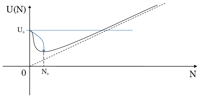
Figure 2: A single possible form of potential energy that allows the existence of an auto-wave mode is shown in black. The arrow shows the path of total energy along which this mode can be set.

Next, consider the case when $\left(k_{1}<0,k_{2}>0\right)$ (Fig. 1(b)). There is no point of minimum in this case, and the potential energy tends to $\left(-\infty\right)$. It means that this system has no equilibrium point, and the autowave mode of nuclear burning is impossible. So this case is not an option for us.

And the last case is $\left(k_{1}<0,k_{2}<0\right)$, which is shown in Fig. 1(c). There is one stationary point in such system – a point of maximum. However, this point is unstable, and the slightest deviation from this point is able to direct the system either towards zero, or to $\left(-\infty\right)$. So in this case the system cannot reach the equilibrium state and stay in it, which means the autowave mode is also not possible.

At this point we can conclude that the only case suitable for our purpose, when ${\tilde{n}}_{Pu}<1$, is the one shown in Fig. 1(a), i.e. when $\left(k_{1}>0,k_{2}>0\right)$.

Let us now consider the situation when the parameter $\tilde{n}_{Pu}$ is greater than one. In this case $k_{1}$ and $k_{3}$ are always greater than zero, and $k_{2}$ is always less than zero. The behavior of the potential energy near the zero point will depend mostly on the exponent with $k_{3}$ factor. This factor is certainly greater than zero when $\tilde{n}_{Pu}>1$, so one would expect a point of minimum on the graph, which is exactly what we need. The behavior of $U\left(N\right)$ will look similar to what is shown in Fig. 1(a). All the arguments related to Fig. 2 are also true for this case. So any case, when $\tilde{n}_{Pu}$ is greater than one, will do.

4 Finding a criterion for the wave velocity

We determined that in order for the autowave mode to be possible, the coefficients $k_{1},k_{2}$ and $k_{3}$ (taking into account the value $\tilde{n}_{Pu}$) must be chosen in such a way, that the potential energy (or its analog) has a point of minimum. The potential force (minus derivative of $U(N)$) in this case will look like Fig. 3.

Figure 3: A schematic representation of the potential force $F\left(N\right)$ (a derivative of $U(N)$ taked with the opposite sign), when the potential energy has a minimum point.

Since in the autowave form the wave propagates over an infinite interval, and there is no explicit dependence on variable $z$ in equation (35), it is always possible to perform a variable substitution that shifts $z$ relative to the function $N$. Let us thus switch to a new variable so that $z=0$ at the point $\frac{N_{0}}{2}$. We replace the function of force by a triangular one (Fig. 4).

Figure 4: Approximate $F\left(N\right)$ which substitutes the real one in Fig. 3.

Next, we try to replace the function of force with two straight lines – one on the negative part of the coordinate axis $z$, and the other on the positive part. If we solve the equation (35) with respect to $N$ with the functions of force in the form of two lines, we obtain two unknown constants for each one of solutions (because the equations are of second order). We adjust these constants to satisfy the boundary conditions. We also hope that the constants adjustment will end up with zeroing out one of them for each solution, since the functions at which they appear will diverge to infinity. Then, if we join the functions and their first derivatives at the point $\frac{N_{0}}{2}$, we would obtain one spare equation, which can be used to find the wave speed.

So, let us first consider the interval $z\in\left(-\infty,0\right)$. Here we make the following substitution:

$$F\left(N\right)=qN,$$ (36)

$$U\left(N\right)=U_{0}-q\frac{{{N^{2}}}}{2},$$ (37)

where $q$ is the slope, and is equal to:

$$q=-{\left.{\frac{{{d^{2}}U\left(N\right)}}{{d{N^{2}}}}}\right|_{N=0}}=-\left({{k_{2}}+\frac{{{k_{3}}}}{{{{\tilde{n}}_{Pu}}^{2}}}}\right)=1.$$ (38)

By substituting (37) into (35) we obtain a homogeneous differential equation of second order, whose solution looks like:

$$N\left(z\right)={C_{1}}\exp\left({{\chi_{1}}z}\right)+{C_{2}}\exp\left({{\chi_{2}}z}\right)$$ (39)

$${\chi_{1,2}}=\frac{1}{2}\left({-\frac{{v{n_{8,-\infty}}}}{\varepsilon}\pm\sqrt{{{\left({\frac{{v{n_{8,-\infty}}}}{\varepsilon}}\right)}^{2}}+4q}}\right).$$ (40)

$\chi_{1}$ is apparently positive, and $\chi_{2}$ is negative. So in order for the $N\left(z\right)$ to converge to $(-\infty)$, $C_{2}$ must be zero. So

$$N\left(z\right)={C_{1}}\exp\left({{\chi_{1}}z}\right).$$ (41)

Now let us consider the interval $z\in\left(0,+\infty\right)$. In this case we make the following substitution:

$$F\left(N\right)=-\left({N-{N_{0}}}\right),$$ (42)

$$U\left(N\right)=U\left({{N_{0}}}\right)-\frac{1}{2}{\left({N-{N_{0}}}\right)^{2}}.$$ (43)

If we substitute the potential energy again into (35), we obtain a similar solution.

$$N\left(z\right)={N_{0}}+{D_{1}}\left(v\right)\exp\left({{\lambda_{1}}\left(v\right)z}\right)+{D_{2}}\left(v\right)\exp\left({{\lambda_{2}}\left(v\right)z}\right),$$ (44)

$${\lambda_{1,2}}=\frac{1}{2}\left({-v\frac{{{n_{8,-\infty}}}}{\varepsilon}\exp\left({-{N_{0}}}\right)\pm\sqrt{{{\left({\frac{{v{n_{8,-\infty}}}}{\varepsilon}\exp\left({-{N_{0}}}\right)}\right)}^{2}}-4}}\right).$$ (45)

As we can see, both $\lambda_{1}$ and $\lambda_{2}$ are negative, so at $(+\infty)$ both constants are at the ”good” exponents (the converging ones), and we cannot zero out any of them. So this way we do not obtain an additional equation, which could be used to find the wave speed.

There is an expression that may be negative under the root in equation (45). Thus, the solution will be the sum of sine and cosine with some coefficients. Since they have a finite period, and the wave propagates on an infinite interval, the derivative will become negative at some point. As we noted above, this would lead us to the negative neutron concentration, which is non-physical. So we require that

$${\left({\frac{{v}}{\varepsilon}\exp\left({-{N_{0}}}\right)}\right)^{2}}-4\geq 0.$$ (46)

Considering this requirement relative to $v$, we obtain the following restriction:

$$v\geq 2\varepsilon\exp\left({{N_{0}}}\right).$$ (47)

It means, that the wave velocity may take a continuous spectrum of values greater than certain minimum value. In the framework of the analogy to the energy conservation law, one might say that the viscosity cannot be less than a certain value. It makes sense, because with higher viscosity the kinetic energy will still dissipate completely to the minimum point, but if the viscosity is not high enough, the body will possess some nonzero speed at the stationary point, which eventually leads to the reverse motion. And as we noted above, the reverse motion is not allowed as non-physical.

Let us check if the speed can take different values. To do this, we choose the parameters so that the potential energy has the point of minimum, and solve the equation (30) numerically. These parameters are: ${{\tilde{n}}_{Pu}}=0.74,\nu=2.8,N_{0}=1.8$, where $N_{0}$ is the point of potential energy minimum. With such values, the condition (47) has the form: $v\geq 15\varepsilon$. Fig. 5 shows the dependences of $N$ on $z$ for different velocities. Comparing it to the potential energy (Fig. 4(a)), one cant notice the following: the coordinate is initially zero, and then it goes to the point of the potential energy minimum. The change in speed, i.e. dissipative force, affects the form of this transition and shifts it in time.

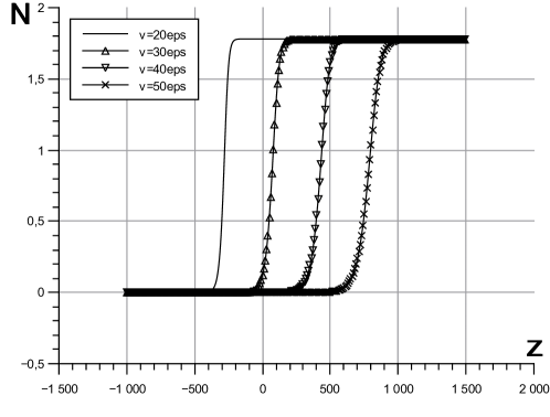
Figure 5: Solutions of Eq. (30) as a function $N(z)$ when a minimum exists in potential energy. The curves are given for different velocities that satisfy the requirement (47).

5 Finding the spectrum of neutron energies, suitable for an auto-wave mode

In order for the autowave to exist, the potential energy (or its analog) must have a point of minimum, and also the wave speed must be such that the kinetic energy is completely dissipated, when the potential energy reaches this minimum point. So now as we realize that, it is interesting to study how the fulfillment of the first condition (existence of the minimum point) depends on the neutrons energy. According to (33) and (34), $U\left(N\right)$ depends on $\nu$ and $\tilde{n}_{Pu}$. These parameters, in turn, depend on the neutron energy. We find the parameter $\tilde{n}_{Pu}$ using Eq. (17) and examine it depending on the neutron energies.

According to [44, 45, 46], the mean number of instantaneous neutrons $\nu$ produced by single fission has the following dependence on energy:

$$\nu\left({Z,A,{E_{n}}}\right)=2.33+0.06\left({2-{{\left({-1}\right)}^{A+1-Z}}-{{\left({-1}\right)}^{Z}}}\right)+0.15\left({Z-92}\right)+\\ +0.02\left({A-235}\right)+\left({0.13+0.006\left({A-235}\right)}\right)\left({{E_{n}}-{E_{threshold}}}\right).$$ (48)

Since we are interested in the average number of neutrons $\nu$ for $Pu^{239}$, we choose the following parameters for the equation (48):

$$A=239,Z=94,E_{threshold}\ =-0.89\left(MeV\right).$$ (49)

So now we know the dependence of the coefficients in the potential energy on the energy of the neutrons. We have to find the entire spectrum of neutron energies at which the potential energy has a point of minimum. It may be done as follows. Break some interval of $N$ (from zero up to a certain maximum value) into sufficiently small segments, and compare the values of $U\left(N\right)$ at three adjacent points. If the value at the middle point is less than those at both ends, then the minimum of the function exists. If we do not find such three points, then there is no minimum at this energy. Having analyzed the entire spectrum of neutron energies this way, we find all the energy intervals with minima.

We show all the neutron energies, for which we found the minimum of potential energy, as a set of points in the graph, where the neutron energy is along the X-axis, and the parameter $\tilde{n}_{Pu}$ is along the Y-axis. Only the values, for which there is a stationary point in the potential energy, are shown.

Fig. 6 shows the values of the parameter $\tilde{n}_{Pu}$ for neutron energies in the range from 0 to 100 eV. We used the dependence of the cross-sections of nuclides on the neutron energy from the database [47]. As seen from Fig. 6 (according to the considerations in Section 3), there are seven regions at about 6-7 eV, 19-21 eV, 34-40 eV, 66-67 eV, 81-82 eV and 90-100 eV, having a minimum of potential energy, which makes the autowave of nuclear fission possible.

Figure 6: The dependence of the parameter $\tilde{n}_{Pu}$ on the energy of neutrons, for the energies, when the potential energy has the point of minimum, and the autowave may exist. The image shows the energy range from 0 to 100 eV.

The entire spectrum of neutron energies is shown in Fig. 7.

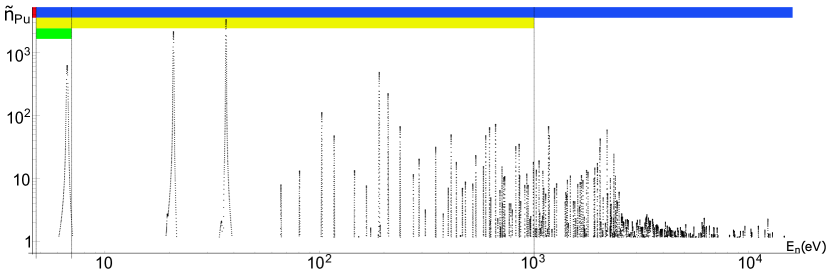
Figure 7: The dependence of the parameter $\tilde{n}_{Pu}$ on the energy of neutrons, for the energies, when the potential energy has the point of minimum, and the existence of an autowave is possible. The upper part of the image marks different neutron energy regions with different colors. Red is for thermal neutrons (there are no points in this area here, so it is barely noticeable), blue is for intermediate neutrons (this area goes beyond the graph and therefore is not depicted fully). There are no points in the region of fast neutrons, so it is not shown here. The additional markings are for resonance neutrons (yellow) and epithermal neutrons (green). This picture embraces all possible points, as the entire region of neutron energies from experimental data [47] was studied

6 Numerical simulation

The system of equations studied above is simplified, and does not fully reflect the physical processes that take place in the reactor core. Let us consider the system of equations given in [32], which is more accurate (though not ideal), and consists of 18 equations. The kinetic equation for the neutron concentration

$$\frac{{\partial\,n\,\left({x,t}\right)}}{{\partial\,t}}=D\,\frac{{{\partial^{2}}\,n\,\left({x,t}\right)}}{{\partial{x^{2}}}}+q\left({x,t}\right),$$ (50)

where $q(x,t)$ is the internal source of neutrons, which has the form:

$$q\left({x,t}\right)=\left[{{\nu^{\left({Pu}\right)}}\left({1-{p^{\left({Pu}\right)}}}\right)-1}\right]\cdot n\left({x,t}\right)\cdot{V_{n}}\cdot\sigma_{f}^{\left({Pu}\right)}\cdot{N_{Pu}}(x,t)+\\ +\left[{{\nu^{\left(5\right)}}\left({1-{p^{\left(5\right)}}}\right)-1}\right]\cdot n(x,t)\cdot{V_{n}}\cdot\sigma_{f}^{\left(5\right)}\cdot{N_{5}}(x,t)+\\ +\ln 2\cdot\sum\limits_{i=1}^{6}{\left[{\frac{{\tilde{N}_{i}^{\left({Pu}\right)}(x,t)}}{{T_{i}^{\left({Pu}\right)}}}+\frac{{\tilde{N}_{i}^{\left(5\right)}(x,t)}}{{T_{i}^{\left(5\right)}}}}\right]}-n(x,t)\cdot{V_{n}}\cdot\sum\limits_{5,8,9,Pu}{\sigma_{c}^{\left(i\right)}\cdot{N_{i}}(x,t)}-\\ -n(x,t)\cdot{V_{n}}\cdot\sum\limits_{i=1}^{6}{\left[{\sigma_{c}^{i\left({Pu}\right)}\cdot\tilde{N}_{i}^{\left({Pu}\right)}(x,t)+\sigma_{c}^{i\left(5\right)}\cdot\tilde{N}_{i}^{\left(5\right)}(x,t)}\right]}-\\ -n(x,t)\cdot{V_{n}}\cdot\sigma_{c}^{eff\left({Pu}\right)}\cdot{{\bar{N}}^{\left({Pu}\right)}}(x,t)-n(x,t)\cdot{V_{n}}\cdot\sigma_{c}^{eff\left(5\right)}\cdot{{\bar{N}}^{\left(5\right)}}(x,t).$$ (51)

In equations (50) and (51) $n(x,t)$ is the neutron concentration; $V_{n}$ is the neutron velocity; $\nu^{(Pu)}$ and $\nu^{(5)}$ are the mean number of instantaneous neutrons per $Pu^{239}$ and ${}^{235}U$ fission respectively. $N_{5}$, $N_{8}$, $N_{9}$ and $N_{Pu}$ are the ${}^{235}U$, ${}^{238}U$, ${}^{239}U$ and ${}^{235}Pu$ concentrations respectively; $\tilde{N}_{i}^{Pu}$ and $\tilde{N}_{i}^{5}$ are the concentrations of fragments with neutron excess, produced due to ${}^{239}Pu$ and ${}^{235}U$ fission respectively; $\overline{N}^{(Pu)}$ and $\overline{N}^{(5)}$ are the concentrations of all the other fission fragments of ${}^{239}Pu$ and ${}^{235}U$ respectively; $\sigma_{c}$ and $\sigma_{f}$ are the microscopic cross-sections of the neutron capture and nuclear fission; the parameters $p_{i}$ $\left(p=\sum\limits_{i=1}^{6}p_{i}\right)$ and $T_{1/2}$ characterize the groups of delayed neutrons. They are well known and presented in [46]. $\sigma_{c}^{eff}$ is some effective microscopic cross-section of neutron capture by fragments.

Let $N_{8,0}$ be the initial ${}^{238}U$ concentration. Then we introduce the new dimensionless concentrations, equal to the old ones divided by $N_{8,0}$.

Then (50), taking into account (51) and using the dimensionless concentrations, becomes:

$$\frac{{\partial\,n\,\left({x,t}\right)}}{{\partial\,t}}=D\,\frac{{{\partial^{2}}\,n\,\left({x,t}\right)}}{{\partial{x^{2}}}}+{V_{n}}\sigma_{f}^{\left({Pu}\right)}\left[{{\nu^{\left({Pu}\right)}}\left({1-{p^{\left({Pu}\right)}}}\right)-1}\right]{N_{8,0}}n\left({x,t}\right){N_{Pu}}(x,t)+\\ +\left[{{\nu^{\left(5\right)}}\left({1-{p^{\left(5\right)}}}\right)-1}\right]{N_{8,0}}{V_{n}}\sigma_{f}^{\left(5\right)}n(x,t){N_{5}}(x,t)+\\ +\ln 2\sum\limits_{i=1}^{6}{\left[{\frac{{\tilde{N}_{i}^{\left({Pu}\right)}(x,t)}}{{T_{i}^{\left({Pu}\right)}}}+\frac{{\tilde{N}_{i}^{\left(5\right)}(x,t)}}{{T_{i}^{\left(5\right)}}}}\right]}-{N_{8,0}}{V_{n}}n(x,t)\sum\limits_{5,8,9,Pu}{\sigma_{c}^{\left(i\right)}{N_{i}}(x,t)}-\\ -{N_{8,0}}{V_{n}}n(x,t)\sum\limits_{i=1}^{6}{\left[{\sigma_{c}^{i\left({Pu}\right)}\tilde{N}_{i}^{\left({Pu}\right)}(x,t)+\sigma_{c}^{i\left(5\right)}\tilde{N}_{i}^{\left(5\right)}(x,t)}\right]}-\\ -{N_{8,0}}{V_{n}}\sigma_{c}^{eff\left({Pu}\right)}n(x,t){{\bar{N}}^{\left({Pu}\right)}}(x,t)-{N_{8,0}}{V_{n}}\sigma_{c}^{eff\left(5\right)}n(x,t){{\bar{N}}^{\left(5\right)}}(x,t).$$ (52)

Then let us switch to dimensionless coordinates. Since

$$V_{n}\sigma_{j}^{(i)}N_{8,0}=\left[\frac{cm}{s}\cdot cm^{2}\cdot\frac{1}{cm^{3}}\right]=\left[\frac{1}{s}\right],$$ (53)

the dimensionless time may be introduced as follows:

$$t_{old}=\frac{1}{V_{n}\sigma_{c}^{(8)}N_{8,0}}t_{new}.$$ (54)

Given (54), the equation (52) takes the form:

$$\frac{{\partial\,n\,\left({x,t}\right)}}{{\partial\,t}}=\,\frac{D}{{{V_{n}}\sigma_{c}^{\left(8\right)}{N_{8,0}}}}\frac{{{\partial^{2}}\,n\,\left({x,t}\right)}}{{\partial{x^{2}}}}+\frac{{\sigma_{f}^{\left({Pu}\right)}}}{{\sigma_{c}^{\left(8\right)}}}\left[{{\nu^{\left({Pu}\right)}}\left({1-{p^{\left({Pu}\right)}}}\right)-1}\right]n\left({x,t}\right){N_{Pu}}(x,t)+\\ +\frac{{\sigma_{f}^{\left(5\right)}}}{{\sigma_{c}^{\left(8\right)}}}\left[{{\nu^{\left(5\right)}}\left({1-{p^{\left(5\right)}}}\right)-1}\right]n(x,t){N_{5}}(x,t)+\\ +\frac{1}{{{V_{n}}\sigma_{c}^{\left(8\right)}{N_{8,0}}}}\ln 2\sum\limits_{i=1}^{6}{\left[{\frac{{\tilde{N}_{i}^{\left({Pu}\right)}(x,t)}}{{T_{i}^{\left({Pu}\right)}}}+\frac{{\tilde{N}_{i}^{\left(5\right)}(x,t)}}{{T_{i}^{\left(5\right)}}}}\right]}-\\ -n(x,t)\sum\limits_{5,8,9,Pu}{\frac{{\sigma_{c}^{\left(i\right)}}}{{\sigma_{c}^{\left(8\right)}}}{N_{i}}(x,t)}-n(x,t)\sum\limits_{i=1}^{6}{\left[{\frac{{\sigma_{c}^{i\left({Pu}\right)}}}{{\sigma_{c}^{\left(8\right)}}}\tilde{N}_{i}^{\left({Pu}\right)}(x,t)+\frac{{\sigma_{c}^{i\left(5\right)}}}{{\sigma_{c}^{\left(8\right)}}}\tilde{N}_{i}^{\left(5\right)}(x,t)}\right]}-\\ -\frac{{\sigma_{c}^{eff\left({Pu}\right)}}}{{\sigma_{c}^{\left(8\right)}}}n(x,t{{\bar{N}}^{\left({Pu}\right)}}(x,t)-\frac{{\sigma_{c}^{eff\left(5\right)}}}{{\sigma_{c}^{\left(8\right)}}}n(x,t){{\bar{N}}^{\left(5\right)}}(x,t).$$ (55)

We introduce the dimensionless coordinate $x$ as follows:

$$x_{old}=\sqrt{\frac{D}{V_{n}\sigma_{c}^{(8)}N_{8,0}}}x_{new}.$$ (56)

Designating

$$\varepsilon_{i}^{\left(j\right)}\equiv\frac{{\sigma_{i}^{\left(j\right)}}}{{\sigma_{c}^{\left(8\right)}}},\beta_{i}^{\left(j\right)}\equiv\frac{{\ln 2}}{{{V_{n}}\sigma_{c}^{\left(8\right)}{N_{8,0}}T_{i}^{\left(j\right)}}}.$$ (57)

and taking into account (56) and (57), we transform equation (55) to the form:

$$\frac{{\partial\,n\,\left({x,t}\right)}}{{\partial\,t}}=\,\frac{{{\partial^{2}}\,n\,\left({x,t}\right)}}{{\partial{x^{2}}}}+\varepsilon_{f}^{\left({Pu}\right)}\left[{{\nu^{\left({Pu}\right)}}\left({1-{p^{\left({Pu}\right)}}}\right)-1}\right]n\left({x,t}\right){N_{Pu}}(x,t)+\\ +\varepsilon_{f}^{\left(5\right)}\left[{{\nu^{\left(5\right)}}\left({1-{p^{\left(5\right)}}}\right)-1}\right]n(x,t){N_{5}}(x,t)+\sum\limits_{i=1}^{6}{\left[{\beta_{i}^{\left({Pu}\right)}\tilde{N}_{i}^{\left({Pu}\right)}(x,t)+\beta_{i}^{\left(5\right)}\tilde{N}_{i}^{\left(5\right)}(x,t)}\right]}-\\ -n(x,t)\sum\limits_{5,8,9,Pu}{\varepsilon_{c}^{\left(i\right)}{N_{i}}(x,t)}-n(x,t)\sum\limits_{i=1}^{6}{\left[{\varepsilon_{c}^{i\left({Pu}\right)}\tilde{N}_{i}^{\left({Pu}\right)}(x,t)+\varepsilon_{c}^{i\left(5\right)}\tilde{N}_{i}^{\left(5\right)}(x,t)}\right]}-\\ -\varepsilon_{c}^{eff\left({Pu}\right)}n(x,t){{\bar{N}}^{\left({Pu}\right)}}(x,t)-\varepsilon_{c}^{eff\left(5\right)}n(x,t){{\bar{N}}^{\left(5\right)}}(x,t).$$ (58)

The same scaling may be applied for the rest 17 equations, eventually yielding:

$$\frac{{\partial\,{N_{8}}\left({x,t}\right)}}{{\partial\,t}} = -\,n\left({x,t}\right)\,\,{N_{8}}\left({x,t}\right),$$ (59)

$$\frac{{\partial\,{N_{9}}\left({x,t}\right)}}{{\partial\,t}} = n\left({x,t}\right)\,\left[{\,{N_{8}}\left({x,t}\right)-\varepsilon_{c}^{\left(9\right)}\,{N_{9}}\left({x,t}\right)}\right]\,-\varepsilon{N_{9}}\left({x,t}\right),$$ (60)

$$\frac{{\partial\,{N_{Pu}}\left({x,t}\right)}}{{\partial\,t}} = \varepsilon{N_{9}}\left({x,t}\right)-\,\left({\varepsilon_{f}^{\left({Pu}\right)}+\varepsilon_{c}^{\left({Pu}\right)}}\right)\,\,n\left({x,t}\right)\,{N_{Pu}}\left({x,t}\right),$$ (61)

$$\frac{{\partial\tilde{N}_{i}^{\left({Pu}\right)}(x,t)}}{{\partial{\kern 1.0pt}t}} = \varepsilon_{f}^{\left({Pu}\right)}p_{i}^{\left({Pu}\right)}n{\kern 1.0pt}\,\left({x,t}\right){\kern 1.0pt}\,{\kern 1.0pt}{N_{Pu}}\left({x,t}\right)-\beta_{i}^{\left({Pu}\right)}\tilde{N}_{i}^{\left({Pu}\right)}\left({x,t}\right)-$$ (62)

$$-\varepsilon_{c}^{eff\left({Pu}\right)}n\left({x,t}\right)\tilde{N}_{i}^{\left({Pu}\right)}\left({x,t}\right),\quad i=1,...,6,$$

$$\frac{{\partial\tilde{N}_{i}^{\left(5\right)}\left({x,t}\right)}}{{\partial{\kern 1.0pt}t}} = {\kern 1.0pt}\varepsilon_{f}^{\left(5\right)}p_{i}^{\left(5\right)}n{\kern 1.0pt}\,\left({x,t}\right){\kern 1.0pt}\,{N_{5}}\left({x,t}\right)-\beta_{i}^{\left(5\right)}\tilde{N}_{i}^{\left(5\right)}(x,t)-$$ (63)

$$-\varepsilon_{c}^{eff\left(5\right)}n\left({x,t}\right)\tilde{N}_{i}^{\left(5\right)}\left({x,t}\right),\quad i=1,...,6$$

$$\frac{{\partial{{\bar{N}}^{\left({Pu}\right)}}\left({x,t}\right)}}{{\partial t}} = \varepsilon_{f}^{\left({Pu}\right)}2\left({1-{p^{\left({Pu}\right)}}}\right)n(x,t){N_{Pu}}(x,t)+$$ (64)

$$+\sum\limits_{i=1}^{6}{\beta_{i}^{\left({Pu}\right)}\tilde{N}_{i}^{\left({Pu}\right)}(x,t)-\varepsilon_{c}^{eff\left({Pu}\right)}n\left({x,t}\right){{\bar{N}}^{\left({Pu}\right)}}\left({x,t}\right)},$$

$$\frac{{\partial{{\bar{N}}^{\left(5\right)}}\left({x,t}\right)}}{{\partial t}} = \varepsilon_{f}^{\left(5\right)}2\left({1-{p^{\left(5\right)}}}\right)n(x,t){N_{5}}(x,t)+$$ (65)

$$+\sum\limits_{i=1}^{6}{\beta_{i}^{\left(5\right)}\tilde{N}_{i}^{\left(5\right)}(x,t)-\varepsilon_{c}^{eff\left(5\right)}n\left({x,t}\right){{\bar{N}}^{\left(5\right)}}\left({x,t}\right)}.$$

In these equations

$$\varepsilon\equiv\frac{1}{{{V_{n}}\sigma_{c}^{\left(8\right)}{N_{8,0}}}}\frac{1}{{{\tau_{\beta}}}}.$$ (66)

Let us set the boundary and initial conditions for these equations. The space is initially filled with ${}^{238}U$ and ${}^{235}U$. So the initial conditions for them are:

$${\left.{{N_{8}}\left({x,t}\right)}\right|_{t=0}} ={\eta_{8}}, {\left.{{N_{5}}\left({x,t}\right)}\right|_{t=0}} ={\eta_{5}},$$ (67)

where $\eta_{8}$ and $\eta_{5}$ are constants adjusting the fuel enrichment ($\eta_{8}+\eta_{5}=1$).

The remaining elements are initially zero, and their boundary conditions:

$${\left.{{N_{9}}\left({x,t}\right)}\right|_{t=0}} =0, {\left.{{N_{Pu}}\left({x,t}\right)}\right|_{t=0}} =0, {\left.{\tilde{N}_{i}^{\left({Pu}\right)}\left({x,t}\right)}\right|_{t=0}} =0,$$ (68)

$${\left.{\tilde{N}_{i}^{\left(5\right)}\left({x,t}\right)}\right|_{t=0}} =0, {\left.{{{\bar{N}}_{Pu}}\left({x,t}\right)}\right|_{t=0}} =0, {\left.{{{\bar{N}}_{5}}\left({x,t}\right)}\right|_{t=0}} =0.$$ (69)

The initial and boundary conditions for neutrons are

$${\left.{n\left({x,t}\right)}\right|_{t=0}} =0, {\left.{n\left({x,t}\right)}\right|_{x=0}} ={n_{0}}\left(t\right),$$ (70)

where ${n_{0}}\left(t\right)$ is some function specifying the number of external neutrons.

For the numerical simulation we use Wolfram Mathematica. We perform the calculations for the energy of neutrons $E_{n}=5.923$ (eV). Unfortunately, this system currently cannot be solved with real parameters, so let us take some approximation. We take $\varepsilon=10^{-3}$. This value is not realistic ($\varepsilon$ is actually about $10^{-14}$), but it is difficult to carry out the numerical calculations with more precise values for our model. The rest of the constants are given below:

$${N_{8,0}}=\frac{{{\rho_{8}}}}{{{\mu_{8}}}}{N_{A}}=\frac{{19}}{{238}}{N_{A}}\left[{\frac{1}{{c{m^{3}}}}}\right];{V_{n}}=2.3957\cdot{10^{6}}\left[{\frac{{cm}}{s}}\right];$$

$${\nu_{Pu}}=2.84;{\nu_{5}}=2.38;{\tau_{\beta}}=3.3days;$$

$$\sigma_{f}^{\left({Pu}\right)}=7.18\left[b\right];\sigma_{c}^{\left({Pu}\right)}=1.57\left[b\right];\sigma_{c}^{\left(8\right)}=6.47\left[b\right];\sigma_{c}^{\left(9\right)}=12.95\left[b\right];$$

$$\sigma_{f}^{\left(5\right)}=7.18\left[b\right];\sigma_{c}^{\left(5\right)}=7.18\left[b\right];{\eta_{8}}=0.9;{\eta_{5}}=0.1;$$

$$\sigma_{c}^{eff\left({Pu}\right)}=011\left[b\right];\sigma_{c}^{i\left({Pu}\right)}=1.0\left[b\right],i=1\ldots 6;$$

$$\sigma_{c}^{eff\left(5\right)}=0.11\left[b\right];\sigma_{c}^{i\left(5\right)}=1.0\left[b\right],i=1\ldots 6;$$

$$p_{1}^{\left({Pu}\right)}=0.0072\cdot{10^{-3}};p_{2}^{\left({Pu}\right)}=0.626\cdot{10^{-3}};p_{3}^{\left({Pu}\right)}=0.444\cdot{10^{-3}};$$

$$p_{4}^{\left({Pu}\right)}=0.685\cdot{10^{-3}};p_{5}^{\left({Pu}\right)}=0.0072\cdot{10^{-3}};p_{6}^{\left({Pu}\right)}=0.0072\cdot{10^{-3}};$$ (71)

$${p^{\left({Pu}\right)}}=\sum\limits_{i=1}^{6}{p_{i}^{\left({Pu}\right)}=0.0021};T_{1}^{\left({Pu}\right)}=56.28\left[s\right];T_{2}^{\left({Pu}\right)}=23.04\left[s\right];$$

$$T_{3}^{\left({Pu}\right)}=5.6\left[s\right];T_{4}^{\left({Pu}\right)}=2.13\left[s\right];T_{5}^{\left({Pu}\right)}=0.62\left[s\right];T_{6}^{\left({Pu}\right)}=0.26\left[s\right];$$

$$p_{1}^{\left(5\right)}=0.21\cdot{10^{-3}};p_{2}^{\left(5\right)}=1.4\cdot{10^{-3}};p_{3}^{\left(5\right)}=1.26\cdot{10^{-3}};$$

$$p_{4}^{\left(5\right)}=2.52\cdot{10^{-3}};p_{5}^{\left(5\right)}=0.74\cdot{10^{-3}};p_{6}^{\left(5\right)}=0.27\cdot{10^{-3}};$$

$${p^{\left(5\right)}}=\sum\limits_{i=1}^{6}{p_{i}^{\left(5\right)}=0.0064};T_{1}^{\left(5\right)}=55.72\left[s\right];T_{2}^{\left(5\right)}=22.72\left[s\right];$$

$$T_{3}^{\left(5\right)}=6.22\left[s\right];T_{4}^{\left(5\right)}=2.3\left[s\right];T_{5}^{\left(5\right)}=0.61\left[s\right];T_{6}^{\left(5\right)}=0.23\left[s\right];$$

A numerical simulation of the wave kinetics was performed for the case of persistent source of external neutrons, as well as for the case of switching the source off after the wave burning is established. Switching off the external source of neutrons allows to test the autowave mode.

When simulating the case of neutron source switching off, the function of external neutrons was given as:

$$n_{0}(t)=3000\cdot t\cdot\exp\left(-0.5\cdot t\right).$$ (72)

Fig. 8 presents the results of numerical simulation (the neutron energy was $E_{n}=5.923$ (eV)) with the external source of neutrons being switched off at some point. The setting of the autowave mode of nuclear burning is confirmed by the fact that starting from a certain moment in time (when the external source of neutrons is already switched off), each subsequent graph differs from the previous only by a shift along the $y$-axis.

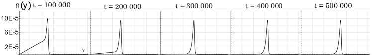
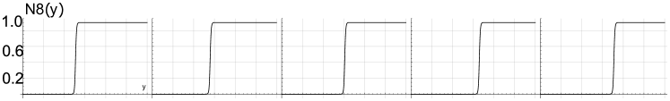
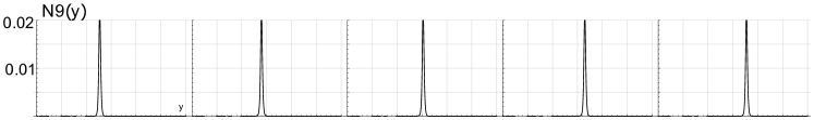
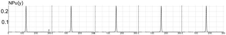
Figure 8: The concentrations of neutrons and nuclides in time from $t=100~{}000$ to $t=500~{}000$.

We also studied the regions of neutron energies for which there was no minimum in potential energy. In such cases the autowave mode did not establish, and the wave faded away after the external source of neutrons was switched off.

7 Conclusions

A kinetic system of equations, describing the wave mode of neutron-nuclear burning in uranium-plutonium medium, is formulated. Its autowave form is also obtained. In contrast to many other papers like [9, 15, 38, 39, 40, 41], we do not neglect the derivative of neutron concentration with respect to time in the neutron diffusion equation. This way we study the non-stationary burning mode.

For the first time a kinetic equation for neutrons is obtained in the form of the energy conservation law for a mechanical system with dissipation, and the mechanical analogy for the fission wave is developed. This allowed to formulate the conditions for the existence of the autowave burning mode, and determine the possible values of the wave speed. We also succeeded in determining the regions of neutron energy, for which the autowave burning is possible. We conclude that in other energy ranges, in which the autowave mode is impossible, the wave of nuclear burning may still be established using the support of an external neutron source.

To confirm the theoretical conclusions, we performed a numerical 1D simulation of the neutron-nuclear burning in uranium-plutonium medium in a single-group diffusion approximation ($E_{n}=5.923$ (eV)). The results of numerical modelling confirm the obtained theoretical conclusions. According to these results, one of the possible areas of autowave burning in the uranium-plutonium medium is the epithermal region of neutron energies (as in [32, 42]). Meanwhile in the region of fast neutrons, the wave burning of the uranium-plutonium medium requires the constant supply of neutrons from an external source, and the wave fades out when the source is switched off.

The discovered burning mode with external support can obviously be used for implementing a traveling-wave reactor, e.g. to stop the burning at any time by switching off the external source of neutrons.

References

• [1] Feoktistov L.P. Safety - key moment in the revival of nuclear power. // Successes of physics sciences.- 1993. - V. 163, No 8. - P. 89-102.(in Russian)
• [2] Dittmar Michael. The future of nuclear energy: facts and fictions. An update using 2009/2010 data.// arXiv:1101.4189v1 [physics.soc-ph]. - 2011. - P. 1-31.
• [3] Rusov V.D., Tarasov V.A., Vaschenko V.N. Traveling-wave nuclear reactor. - Kyiv: Publishing group ”A.C.C.”. - 2013. - 156 p.
• [4] Babenko V.A., Enkovskii L.L., Pavlovich V.N. Nuclear power engineering. Trends in the world and the peculiarities of Ukraine. // Physics of Elementary Particles and the Atomic Nucleus. - 2007. - V. 37. - No 6. - p. 1517-1580.(in Russian)
• [5] Stacey W.M. Capabilities of a DT Tokamak Fusion Neutron Source for Driving a Spent Nuclear Fuel Transmutation Reactor. // Nuclear Fusion. - 2001. - Vol. 41. - P. 135-143.
• [6] Hofman E. A. and Stacey W. M. Nuclear design and analysis of the fusion transmutation of waste reactor. // Fusion Science and Technology. - January 2004. - Vol. 45. - P. 51-54.
• [7] Alejandro Clausse, Leopoldo Soto, Carlos Friedli, Luis Altamirano. Feasibility study of a hybrid subcritical fission system driven by Plasma-Focus fusion neutrons. // Annals of Nuclear Energy. - 2015. – Vol. 78. - P. 10–14.
• [8] Xianjun Zheng, Baiquan Deng, Wei Ou, Fujun Gou. Conversion of U-238 and Th-232 Using a Fusion Neutron Source. // World Journal of Nuclear Science and Technology. - 2014. - Vol. 4. - P. 222-227.
• [9] Feoktoistov L.P. Neutron-fission wave // Reports of the Academy of Sciences of the USSR. - 1989. - Vol. 309, No 4. - p. 864-867.(in Russian)
• [10] Teller, E., Ishikawa, M., Wood, L., Hyde, R., Nuckolls, J., 1996. Completely automated nuclear reactors for long-term operation II: Toward a concept-level point-design of a high-temperature, gas-cooled central power station system, part II, in: Proceedings of the International Conference on Emerging Nuclear Energy Systems, ICENES’96, Obninsk, Russian Federation, Obninsk, Russian Federation, Obninsk, Russian Federation. pp. 123–127. Also available from Lawrence Livermore National Laboratory, California, publication UCRL-JC-122708-RT2.
• [11] Goldin V.Ya., Sosnin N.V., Troschiev Yu.V. “Fast reactor in self-regulation mode of the 2nd kind // Russian Acad.Sci. Reports, Mathematical Physics, Vol. 358 (1998) No 6, pp. 747-748.
• [12] A. I. Akhiezer, D. P. Belozorov, F. S. Rofe-Beketov, L. N. Davydov, and Spolnik Z. A. On the theory of propagation of chain nuclear reaction in diffusion approximation. // Yad. Fiz., 62: 1567–1575, 1999.
• [13] H. Sekimoto, K. Ryu, and Y. Yoshimura. CANDLE: The new burnup strategy. // Nuclear science and engineering, Vol.139, pp. 306–317, 2001.
• [14] H. Sekimoto and K. Ryu. A new reactor burnup concept ”CANDLE”.// PHYSOR 2000, Pittsburgh, May 7-11 2000.
• [15] Ershov, A.P., Anisichkin, V.F., 2003. Natural neutron-fission wave. // Combustion, Explosion, and Shock Waves 39 (2).(in Russian)
• [16] V. Rusov, V. Pavlovich, V. Vaschenko, V. Tarasov, T. Zelentsova, V. Bolshakov, D. Litvinov, S. Kosenko, and O. Byegunova. Geoantineutrino spectrum and slow nuclear burning on the boundary of the liquid and solid phases of the Earth’s core. // J. Geophys. Res., 112:B09203, 2007. 10.1029/2005JB004212
• [17] J. Gilleland, C. Ahlfeld, D. Dadiomov, R. Hyde, Y. Ishikawa, D. McAlees, J. McWhirter, N. Myhrvold, J. Nuckolls, A. Odedra, K. Weaver, C. Whitmer, L. Wood, and G. Zimmerman. Novel Reactor Designs to Burn Non-Fissile Fuels. // International Congress on Advances in Nuclear Power Plants (ICAPP 2008), American Nuclear Society, Anaheim, CA, Paper No. 8319. – 2008.
• [18] Kevan D. Weaver, J. Gilleland, C. Ahlfeld, C. Whitmer, G. A. Zimmerman, A Once-Through Fuel Cycle for Fast Reactors. // Journal of Engineering for Gas Turbines and Power. - 2010. - Vol. 132. - P. 1-6.
• [19] T. Ellis, R. Petroski, P. Hejzlar, G. Zimmerman, et al. Traveling-wave Reactors: A Truly Sustainable and Full-Scale Resource for Global Energy Needs. // 2010 International Congress on Advances in Nuclear Power Plants (ICAPP 2010), San Diego, CA, USA, Paper No. 10189.- 2010.
• [20] Ahlfeld C. E. et al. Traveling wave nuclear fission reactor, fuel assembly, and method of controlling burnup therein. // Patent Application Publication No.: US 20100254501. - Jul. 10, 2010.
• [21] Xue-Nong Chen, Werner Maschek. Transverse buckling effects on solitary burn-up waves. // Annals of Nuclear Energy. - 2005. - Vol. 47. - P. 1301-1313.
• [22] Xue-Nong Chen, Edgar Kiefhaber, Dalin Zhang, Werner Maschek. Fundamental solution of nuclear solitary wave. // Energy Conversion and Management. - 2012. - Vol. 59. - P. 40–49.
• [23] Xue-Nong Chen and Edgar Kiefhaber. Asymptotic Solutions of Serial Radial Fuel Shuffling. // Energies. - 2015. - 8. - P. 1 – 21; doi: 10.3390/en80x000x.
• [24] Jinfeng Huang, Jianlong Han, Xiangzhou Cai, Yuwen Ma, Xiaoxiao Li, Chunyan Zou, Chenggang Yu, Jingen Chen. Breed-and-burn strategy in a fast reactor with optimized starter fuel // Progress in Nuclear Energy. - 2015. - Vol. 85. - P. 11 – 16.
• [25] Gann V.V. Benchmark of a traveling wave reactor using MCNPX code. /Gann V.V., Abdullaev A.M., Gann A.V. // Kharkiv: National Scientific Centre “Kharkiv Institute of Physics and Technology”. - 2010. -P. 24.(in Russian)
• [26] Osborne A.G. et al. Comparison of neutron diffusion and Monte Carlo simulations of a fission wave. // Annals of Nuclear Energy. - 2013. - 62. - P. 269-273.
• [27] Kim T.K. and Taiwo T.A. Fuel Cycle Analysis of Once-Through Nuclear Systems. Fuel Cycle Research and Development. // Argonne National Laboratory, report ANL-FCRD-308 of the U.S. Department of Energy Systems Analysis Campaign - 2010. - P. 1-53.
• [28] Osborne A.G., Deinert M.R. Neutron damage reduction in a traveling wave reactor. // Proceedings of Physor 2012, Knoxville, TN, April 15-20, 2012.
• [29] V. D. Rusov, V. A. Tarasov, I. V. Sharf, V. M. Vaschenko, E. P. Linnik, T. N. Zelentsova, M. E. Beglaryan, S. A. Chernegenko et al. On some fundamental peculiarities of the traveling wave reactor operation. Science and Technology of Nuclear Installations. - 2015. - Vol. 2015. - P. 1 – 23; doi: 10.1155/2015/703069; arXiv:1207.3695v1 [nucl-th]
• [30] Staffan Qvist, Jason Hou, Ehud Greenspan. Design and performance of 2D and 3D-shuffled breed-and-burn cores. Annals of Nuclear Energy. - 2015. - Vol. 85. - P. 93 – 114.
• [31] Jason (Jia) Hou, Staffan Qvist, Roger Kellogg, Ehud Greenspan. 3D in-core fuel management optimization for breed-and-burn reactors. // Progress in Nuclear Energy. - 2016. - Vol. 88. - P. 58 – 74.
• [32] Rusov V.D. Ultraslow wave nuclear burning of uranium-plutonium fissile medium on epithermal neutrons/ V.D. Rusov, V.A. Tarasov, M.V. Eingorn, S.A. Chernezhenko et al. // Progress in Nuclear Energy. - 2015. - Vol. 83. - P. 105 – 122.
• [33] V.D. Rusov, E.P. Linnik, V.A. Tarasov, T.N. Zelentsova, V.N. Vaschenko, S.I. Kosenko, M.E. Beglaryan, S.A. Chernezhenko et al. Traveling Wave Reactor and Condition of Existence of Nuclear Burning Soliton-like Wave in Neutron-Multiplicating Media. // Energies (Special Issue “Advances in Nuclear Energy”). - 2011. - 4. - P. 1337 – 1361; doi: 10.3390/en4091337.
• [34] V.D. Rusov, D.A. Litvinov, E.P. Linnik, V.M. Vaschenko, T.N. Zelentsova, M.E. Beglaryan, V.A. Tarasov, S.A. Chernegenko et al. KamLand-Experiment and Soliton-Like Nuclear Georeactor. Part 1. Comparison of the Theory with Experiment. // Journal of Modern Physics, 2013, No 4, p. 528-550.
• [35] V.D. Rusov, V.A. Tarasov, V.M. Vaschenko, E.P. Linnik, T.N. Zelentsova, M.E. Beglaryan, S.A. Chernegenko, et al. Fukushima plutonium effect and blow-up regimes in neutron-multiplying media. // World Journal of Nuclear Science and Technology, 2013, No 3, p. 9-18.
• [36] Fomin S.P. Investigation of self-organization of the non-linear nuclear burning regime in fast neutron reactors. / S.P. Fomin, Yu. P. Mel‘nik, V.V. Pilipenko, N.F. Shul‘ga. // Annals of Nuclear Energy. - 2005. - V. 32. - P. 1435 - 1456.
• [37] Fomin S., Mel’nik Yu., Pilipenko V., Shul’ga N. Initia-tion and propagation of nuclear burning wave in fast reactor // Progress in Nuclear Energy. - 2008. - Vol. 50. - P. 163 - 169.
• [38] Pavlovich V.N., Khotyaintseva E.N., Rusov V.D. et al. Reactor operating on a slow wave of nuclear fission // Energy (2007) 102: 181. doi:10.1007/s10512-007-0027-x.(in Russian)
• [39] Khotyayintsev V.M., Pavlovych V.M., Khotyayintseva O.M. Travelling-wave reactor: velocity formation mechanisms. // PHYSOR 2010, on CD-ROM.
• [40] Khotyayintseva O.M., Khotyayintsev V.M., Pavlovych V.M., Temperature feedback effect to stationary wave of nuclear fusion. // Nuclear Physics and Atomic Energy 15(1):26-34 · January 2014. (in Russian)
• [41] Khotyayintsev V.M., Khotyayintseva O.M., Aksonov A.V. et al. Velocity characteristic and stability of wave solutions for a CANDLE reactor with thermal feed-back. // Annals of Nuclear Energy. - 2015. - Vol. 85C. - P. 337 - 345.
• [42] Tarasov V.A., Vaschenko V.N., Chernegenko S.A. Nuclear reactor on a traveling wave: ultra-slow wave neutron-nuclear combustion on epithermal neutrons and regimes with peaking in a uranium-plutonium fission medium. // Kyiv: Publishing group ”A.C.C.”. - 2016.(in Russian)
• [43] Cerullo Nicola. The use of GFR dedicated assemblies in the framework of advanced symbiotic fuel cycles: An innovative way to minimize long-term spent fuel radiotaxicity. / Nicola Cerullo, Davide Chersola, Guglielmo Lomonaco, Riccardo Marotta. // Twelfth information exchange meeting on actinide and fission product partitioning and transmutation, OECD 2013. - 2013. - P. 10.
• [44] Weinberg A.M. and Wigner E.P. The Physical Theory of Neutron Chain Reactors. – Chicago: The University of Chicago Press. – 1958. – 801 p.
• [45] Pavlovych V.M. Physics of nuclear reactors. // Chernobyl: Nuclear station security and safety problem research institute. - 2009. - P. 224.(in Ukrainian)
• [46] Bartolomey, G.G., Bat’, G.A., Baibakov, V.D., Altukhov, M.S., 1989. Basic Theory and Methods of Nuclear Power Installations Calculation. Energoatomizdat, Moscow, p. 512 (in Russian).
• [47] Chadwick M.B., Herman M., Obložinský P. et al. ENDF/B-VII.1 Nuclear Data for Science and Technology: Cross Sections, Covariances, Fission Product Yields and Decay Data // Nuclear Data Sheets. - 2011. - Vol. 112, Iss. 12. - P. 2887 - 2996.