Analytic components for the hadronic total cross-section: Fractional calculus and Mellin transform

Abstract

In high-energy hadron-hadron collisions, the dependence of the total cross-section ($\sigma_{tot}$) with the energy still constitutes an open problem for QCD. Phenomenological analyses usually relies on analytic parameterizations provided by the Regge-Gribov formalism and fits to the experimental data. In this framework, the singularities of the scattering amplitude in the complex angular momentum plane determine the asymptotic behavior of $\sigma_{tot}$ in terms of the energy. Usual applications connect simple and triple pole singularities with asymptotic power and logarithmic-squared functions of the energy, respectively. More restrict applications have considered as a leading component for $\sigma_{tot}$ an empirical function consisting of a logarithmic raised to a real exponent, which is treated as a free fit parameter. With this function, data reductions lead to good descriptions of the experimental data and real (not integer) values of the exponent. In this paper, making use of two independent formalisms (fractional calculus and Mellin transform), we first show that the singularity associated with this empirical function is a branch point and then we explore the mathematical consequences of the result and possible physical interpretations. After reviewing the determination of the singularities from asymptotic forms of interest through the Mellin transform, we demonstrate that the same analytic results can be obtained by means of the Caputo fractional derivative, leading, therefore, to fractional calculus interpretations. Besides correlating Mellin transform, non-local fractional derivatives and exploring the generalization from integer to real exponents and derivative orders, this fractional calculus result may provide insights for physical interpretations on the asymptotic rise of $\sigma_{tot}$. We also illustrate the applicability of the parameterizations by means of novel fits to $\sigma_{tot}$ data.

Keywords: Fractional calculus, Caputo fractional derivative, Mellin transform, total cross-sections, asymptotic problems and properties

Contents

1. Introduction

2. Analytic Parametrization and Mellin Transform

2.1 Analytic Parametrization and a Canonical Function

2.2 Mellin Transform and Singularities

3. Fractional Calculus and the Caputo Derivative

3.1 Introduction and Motivation

3.2 Fractional Calculus

3.3 Fractional Integral Operator

3.3.1 Fractional Integral in the Riemann-Liouville Sense

3.4 Fractional Derivative Operators

3.4.1 Fractional Derivative in the Riemann-Liouville Sense

3.4.2 Fractional Derivative in the Caputo Sense

3.5 Connecting Asymptotic Forms and Singularities

4. Discussion

5. Summary, Conclusions and Final Remarks

Appendix A Total Cross Section and the Regge-Gribov Formalism

A.1 Total Hadronic Cross Section

A.2 Basic Phenomenological Concepts

A.3 Analytic Parameterizations

Appendix B Data Reductions to $pp$ and $\bar{p}p$ Total Cross-Sections

B.1 Fit Procedures and Results

B.2 Discussion on the Fit Results

1 Introduction

High-Energy Physics deals with the study of the inner structure of matter, the sub-nuclear particles and their interactions [1]. The main experimental tool consists of collision of these particles (protons, pions, kaons,…) at high energies, namely center-of-mass energies above 10 $m_{p}\sim$ 10 GeV, where $m_{p}$ is the proton mass. Presently, the highest energies reached in accelerators, with particles and anti-particles, concern proton-proton ($pp$) and antiproton-proton ($\bar{p}p$) collisions at 8 TeV and $\sim$ 2 TeV, respectively. These strong (hadronic) interactions are expected to be described by the Quantum Chromodynamics (QCD), a non-Abelian gauge field theory [1, 2].

Among the physical observables characterizing a particle collision process, the total cross section ($\sigma_{tot}$) plays a central role. On the one hand, beyond being physically related with the probability and also an effective area of interaction, a large amount of experimental data, as a function of the collision energy, has been obtained from several scattering processes, providing solid information on the empirical behavior of this quantity. On the other hand, however, the theoretical description of its dependence on the energy constitute a long standing challenge for QCD. Indeed, the total cross-section is obtained from the imaginary part of the forward elastic scattering amplitude $\mathcal{A}(s,t)$ through the optical theorem, which at high energies reads [3]

$$\sigma_{\mathrm{tot}}(s)=\frac{\mathrm{Im}\,\mathcal{A}(s,t=0)}{s},$$ (1)

where $s$ and $t$ are the energy and momentum transfer squared in the center of mass system (Mandestam variables) and $t=0$ means the forward direction. Therefore, the determination of $\sigma_{tot}(s)$ demands a theoretical result for the forward elastic amplitude in terms of the energy, valid in all region above the physical threshold. However, as a soft scattering state (large distances and small momentum transfer), the perturbative QCD techniques cannot be applied due to the increase of the coupling constant as the momentum transfer decreases, namely the dynamics involved in the elastic scattering is intrinsically nonperturbative. Presently, the crucial point concerns the lack of a nonperturbative framework able to provide from the first principles of QCD a description of $\sigma_{tot}(s)$ for all $s$.

A historical and formal result on the rise of $\sigma_{tot}(s)$, at the asymptotic energy region ($s\rightarrow\infty$), is the upper bound derived by Froissart and Martin (FM) [4, 5, 6, 7]

$$\sigma_{tot}(s)<c\ln^{2}(s/s_{0}),$$ (2)

where $s_{0}$ is an energy scale and $c$ a constant. More recently, 2011, and yet in a formal (theoretical) context, the possibility of a rise of $\sigma_{tot}(s)$ faster than the above log-squared bound, without violating unitarity, was discussed by Azimov [8].

Beyond specific phenomenological models [9, 10], the behavior of $\sigma_{tot}(s)$ is usually investigated by means of forward amplitude analyses, consisting of tests of different analytic parameterizations for $\sigma_{tot}(s)$ and the $\rho$ parameter (the ratio between the real and imaginary parts of the forward amplitude) and fits to the experimental data. The analytic parameterizations are constructed on the bases of $S$-Matrix and Regge-Gribov formalism [3, 11, 12]. In this context, the singularities of the scattering amplitude in the complex angular momentum $J$-plane ($t$-channel) determine the asymptotic energy dependence of the total cross-section ($s$-channel). As we shall discuss, simple, double and triple pole singularities result in power, logarithmic and logarithmic-squared laws, respectively, for $\sigma_{tot}(s)$. The standard picture indicates a leading log-squared dependence at the highest energies [13, 14, 15, 16], in accordance with the FM bound, Eq. (2) and associated, therefore, with a triple pole singularity in the complex $J$-plane.

Beyond this log-squared, $\ln^{2}(s/s_{0})$ (L2), leading dependence, other amplitude analyses have considered an empirical leading log-raised-to-gamma form, $\ln^{\gamma}(s/s_{0})$ (L$\gamma$), with $\gamma$ as a real free fit parameter, a parametrization introduced by Amaldi et al. in 1977 [17]. Besides providing equivalent descriptions of the experimental data available [17, 18, 19], including the recent LHC data [20, 21, 22, 23, 24, 25], this empirical parametrization is also useful as a quantitative check on the behavior of $\sigma_{tot}(s)$ (dictated by the experimental data) in respect the FM bound, namely how close to 2 the extracted $\gamma$-value lies: equal 2, below or above 2.

In this respect, although based on different approaches and datasets, the analyses quoted in the previous paragraph, suggest $\gamma$-values exceeding 2 (typically $2.2-2.3$ in [22, 23]), which contrasts with the result obtained by the COMPAS Group, favoring a $\gamma$-value below 2: $1.98\pm 0.01$ [15, 16]. To our purposes, the main point to notice is: once amplitude analyses with the exponent $\gamma$ treated as a free fit parameter have favored real (not integer) and positive $\gamma$ values, the associated singularity may not be a triple pole.

In spite of the aforementioned useful properties, the L$\gamma$ law has had only an empirical basis, without further justification or devised connections with a formal approach and that is the point we are interested in here, at least in a mathematical context. Taking account of the absence of a pure nonperturbative QCD description of $\sigma_{tot}(s)$, we explore some mathematical aspects related to the L$\gamma$ law, looking for possible connections with the Regge-Gribov formalism. With that in mind, we shall consider two independent frameworks: the Fractional Calculus (which is a generalization of the classical integer order Calculus to real or complex order) [26, 27, 28] and the Mellin Integral Transform (which can connect asymptotic forms of real valued functions of real argument, with the singularities of the transformed function in a complex plane) [29, 30, 31].

Our specific goals are: (1) in a kind of inverse approach, to review the determination of the singularities associated with the asymptotic analytic components of $\sigma_{tot}(s)$ by means of the Mellin transform, showing, in particular, that the L$\gamma$ law, with $\gamma>0$, real and not integer, can be associated with a branch point singularity; (2) to demonstrate that the same analytic results can be obtained in a fractional calculus approach, through the Caputo fractional derivative [32, 33]; (3) to explore the possible connections among the Mellin transform, the nonlocal character of the Caputo fractional derivative (memory effects) and the Regge-Gribov formalism. In addition, we also illustrate the applicability of the full parametrization (including lower energy components), by developing novel fits to all the $\sigma_{tot}$ data presently available from $pp$ and $\bar{p}p$ scattering in the energy region 5 GeV - 8 TeV, which lead to real (not integer) $\gamma$ value exceeding 2: $\gamma\approx 2.2\pm 0.1$.

The paper is organized as follows. In Sect. 2, after identifying a characteristic function in the analytic parameterizations for $\sigma_{tot}(s)$, we review the use of the Mellin transform in the determination of the associated singularities. In Sect. 3, after recalling some basic concepts on Fractional Calculus, we develop the novel calculations connecting the characteristic function with the corresponding singularities. Sect. 4 is devoted to a discussion on all the obtained results and possible physical interpretations associated. Our conclusions and final remarks are the contents of Sect. 5. In Appendix A, we refer to the $\sigma_{tot}$ concept and the experimental data presently available at the highest energies, presenting also a short review on the construction of the analytic parametrization for $\sigma_{tot}(s)$ in the Regge-Gribov context. In Appendix B, we illustrate the applicability of the parameterizations by means of novel fits to $\sigma_{tot}$ data from $pp$ and $\bar{p}p$ scattering.

2 Analytic Parametrization and Mellin Transform

After identifying a characteristic function of the energy, in the asymptotic parameterizations for the total cross section, we review the determination of the corresponding singularities in the complex $J$-plane by means of the Mellin transform; see, for example, [3] (Appendix B ), [34] (Sect. 2.8), [35] (Sect. 3.6).

2.1 Analytic Parametrization and a Canonical Function

As reviewed in Appendix A (and quoted references), the analytic parametrization for the total cross section, introduced by Amaldi et al. [17] and used in several analyses [18, 19, 20, 21, 22, 23, 24, 25], can be expressed by

$$\sigma_{tot}(s)=a_{1}[\tilde{s}]^{-b_{1}}+\tau a_{2}[\tilde{s}]^{-b_{2}}+A+B\ln^{\gamma}(\tilde{s}),$$ (3)

where $a_{i},b_{i},i=1,2$, $A$, $B$, $\gamma$ are real parameters, $\tau=-1$ for $pp$ and $\tau=+1$ for $\bar{p}p$ and

$$\tilde{s}=\frac{s}{s_{0}},$$ (4)

with $s_{0}$ an energy scale.

For our purposes it is important to note [34, 35, 36] that all the components in Eq. (3) are particular cases of a canonical (dimensionless) function given by

$$f_{ca}(\tilde{s})=\tilde{s}^{\alpha}\ln^{\gamma}(\tilde{s}),$$ (5)

where, for short, we denote here $\alpha_{0}-1\equiv\alpha$, with $\alpha_{0}$ the intercept of the trajectory (see Appendix A.2). Indeed, for $\gamma=0$ and different $\alpha$ values, we have all the power (and constant) laws in Eq. (3) associated with Reggeons and Pomerons. For $\alpha=0$ and $\gamma=1,2$ the logarithmic dependences representing the Pomeron are obtained (Appendix B). In case of $\gamma$ a real (not integer) parameter ($\alpha=0$ for the L$\gamma$ law), the association with a cross section demands real values for the logarithmic function and therefore we have an additional condition:

$$\tilde{s}\geq 1\quad\mathrm{for\ real\ (not\ integer)}\ \gamma$$

In the next Subsection we shall obtain the singularities associated with the asymptotic canonical function Eq. (5) by means of the Mellin transform.

2.2 Mellin Transform and Singularities

The Mellin transform connects a real valued function $\phi(t)$, defined on the real axis $t\in(0,\infty)$, with a function $\Phi(z)$, defined in the complex plane $z=x+iy$, by the relation [29, 30]:

$$\Phi(z)=\int_{0}^{\infty}t^{z-1}\phi(t)dt\equiv\mathcal{M}[\phi(t),z].$$ (6)

The integral exists in the region $a<x<b$, named strip of definition (or fundamental strip), where $a$ and $b$ depend on $\phi(t)$.

For our purposes, the main ingredient here is the correspondence between the asymptotic expansion of the function $\phi(t)$ and the singularities of the transformed function $\Phi(z)$ in the complex $z$-plane [30, 31]. To this end, from the definition, it is straightforward to show that $\Phi(-z)=\mathcal{M}[\phi(1/t),z]$, which allows to change the kernel to $t^{-z-1}$, useful for identifying the singularity on the $z$-plane. Our aim is to use as input the canonical function Eq. (5), obtaining the associated singularities.

Firstly, by changing the variable $t=1/\tilde{s}$ in Eq. (6) and for $\Phi(-z)\equiv F(J)$ (with $J$ the complex angular momentum), we obtain

$$F(J)=\int_{0}^{\infty}\tilde{s}^{-J-1}\phi(1/\tilde{s})d\tilde{s}.$$ (7)

In order to treat the general case, where $\gamma$ can take on real (not integer) values, we connect $\phi(1/\tilde{s})$ with the canonical function, Eq. (5), by means of a Heaviside function (note the inversion in the independent variables),

$$\phi(1/\tilde{s})\equiv\theta(\tilde{s}-1)f_{ca}(\tilde{s}),$$

leading to

$$F(J)=\int_{1}^{\infty}\tilde{s}^{\alpha-J-1}\ln^{\gamma}(\tilde{s})d\tilde{s}.$$ (8)

At last, with a change of variable, $\tilde{s}=1/\xi$, the above integral reads

$$F(J)=\int_{0}^{1}\xi^{(J-\alpha)-1}\ln^{\gamma}\left(\frac{1}{\xi}\right)d\xi$$ (9)

and from [37] (page 550, formula 4.272.6), we obtain the final result

$$F(J)=\frac{\Gamma(\gamma+1)}{(J-\alpha)^{\gamma+1}},$$ (10)

for $\gamma>-1$, Re$[J-\alpha]>0$ and where $\Gamma$ is the Euler gamma function.

We see that, for $\gamma=n=0,1,2$, the corresponding singularities at $J=\alpha$ are poles of order $n+1$ and for real (not integer) $\gamma>0$ values, the associated singularities are branch points. In the next Section, we shall correlate the results given by Eqs. (5) and (10) in a completely different mathematical context, which shall provide further interesting interpretations.

3 Fractional Calculus and the Caputo Derivative

3.1 Introduction and Motivation

As we have mentioned (see Appendix A and quoted references), in the Regge-Gribov formalism, a simple pole in the complex angular momentum plane is associated with a power law for the total cross section as a function of the energy:

$$\frac{1}{J-\alpha}\qquad\Longleftrightarrow\qquad\tilde{s}^{\alpha}.$$

Note that these are particular cases of Eqs. (5) and (10) for $\gamma=0$.

As discussed in [11] (Sect. 2.3), higher order poles can be generated by derivatives of the simple pole,

$$\frac{d^{n}}{d\alpha^{n}}\left(\frac{1}{J-\alpha}\right)=\frac{n!}{(J-\alpha)^{n+1}},\quad n=1,2,...,$$ (11)

with $n+1\equiv N$ the order of the pole. Translating this derivative to the power-law, we obtain

$$\frac{d^{n}}{d\alpha^{n}}\tilde{s}^{\alpha}=\tilde{s}^{\alpha}\ln^{n}(\tilde{s}),\quad n=1,2,...$$ (12)

We notice that Eqs. (11) and (12) correspond to particular cases of Eqs. (5) and (10) for poles singularities and/or integer powers in the logarithmic functions. Moreover, from Eqs. (11) and (12), this “integer" character is associated with the integer order of the derivatives respect to $\alpha$. It seems, therefore, natural to look for a generalization of this result with bases on extensions of integer to real orders, namely the Fractional Calculus [26, 27, 28].

In this section, after reviewing some basic definitions of Fractional Calculus and introducing the fractional derivative in the Caputo sense [32, 33], we generalize Eqs. (11) and (12) for a real order (not integer) derivative, obtaining Eqs. (5) and (10). Discussions on the implications of this result and possible physical interpretations are presented in Sect. 4.

3.2 Fractional Calculus

In 1695, after a letter by l’Hôpital to Leibniz, where the former questioned the meaning of a semi-derivative of $y(x)$ (dependent variable) in relation to $x$ (independent variable), fractional calculus was born [38]. Although historically associated to a semi-derivative (fractional order), the true name fractional calculus concerns calculus of arbitrary order. The first attempt to unify several areas involved with the fractional calculus, took place in the first International Congress, realized at New Haven, in 1974 [39]. The fractional calculus has then grown and several definitions involving the integral operator and derivative operators have appeared in the literature [40].

We note that there are more than one way to introduce the concept of fractional derivatives, one of them, by means of the corresponding integral operator with a singular kernel [41, 42] and, in some papers, by means of a convenient limit process [43, 44] and more recently through an integral with a nonsingular kernel [45, 46]. On the other hand, in a recent and interesting paper [47] the authors discuss a criterion that an operator must satisfy to be interpreted as a fractional derivative operator, similar to the one proposed by Ross [48].

Here, we will employ the first approach, i.e., using the fractional integral operator, we introduce the fractional differential operator. To this end, we first treat the fractional integral operator and after that, the fractional derivative operator, in the Caputo sense, only.

3.3 Fractional Integral Operator

There are several ways to introduce a fractional operator of arbitrary order, we mention two of them, i.e., in the Riemann-Liouville sense and their variations [49] and in the Hadamard sense [50], each one defined by a particular class of functions where the operators can be applied. We will only consider spaces where the functions are continuous or continuous by parts [51]. Thus, we introduce the Riemann-Liouville fractional integral and the Caputo fractional derivative, defined in terms of the Riemann-Liouville fractional integral.

3.3.1 Fractional Integral in the Riemann-Liouville Sense

Let $\Omega=[a,b]$ with $-\infty<a<b<\infty$ be a finite interval on the real axis $\mathbb{R}$. The integral of arbitrary order in the Riemann-Liouville sense, of order $\mu\in\mathbb{C}$, with $\mbox{Re}(\mu)>0$, denoted by, $(J_{a+}^{\mu}f)(x)\equiv{}_{a}J_{x}^{\mu}f(x)$ is defined by:

$$(J_{a+}^{\mu}f)(x):=\frac{1}{\Gamma(\mu)}\int_{a}^{x}\frac{f(t)dt}{(x-t)^{1-\mu}},\qquad x>a,\qquad\mbox{Re}(\mu)>0.$$ (13)

This integral is the so-called fractional integral in the Riemann-Liouville sense on the left. We can introduce another one on the right [49]. The integral of arbitrary order in the Riemann-Liouville sense, can be extended on the real axis $\mathbb{R}$.

3.4 Fractional Derivative Operators

As we already said, we are interested in the fractional derivative in the Caputo sense, but as this definition can be done in terms of the fractional derivative in the Riemann-Liouville sense, we first introduce the fractional derivative in the Riemann-Liouville sense by means of the Riemann-Liouville integral.

3.4.1 Fractional Derivative in the Riemann-Liouville Sense

The Riemann-Liouville derivative in a finite interval on the real axis, of order $\mu\in\mathbb{C}$ with $\mbox{Re}(\mu)\geq 0$, denoted by, ${\mbox{D}}_{a+}^{\mu}y$ is defined by

$$({\mbox{D}}_{a+}^{\mu}y)(x):=\left(\frac{d}{dx}\right)^{n}\left(J_{a+}^{n-\mu}y\right)(x)$$

with $n=[\mbox{Re}(\mu)]+1;\,\,x>a$, where $[\mbox{Re}(\mu)]$ means the integer part of $\mbox{Re}(\mu)$.

Also, this derivative is named fractional derivative in the Riemann-Liouville sense on the left. Analogously, we can define another one on the right [49]. The derivative of an arbitrary order in the Riemann-Liouville sense, can be extended on the real axis $\mathbb{R}$. In words, the fractional derivative in the Riemann-Liouville sense, is equal to the derivative of integer order of a fractional integral.

3.4.2 Fractional Derivative in the Caputo Sense

Let $[a,b]$ be a finite interval on the real axis $\mathbb{R}$ and ${\mbox{D}}_{a+}^{\mu}[y(t)](x)\equiv({\mbox{D}}_{a+}^{\mu}y)(x)$ be the derivative in the Riemann-Liouville sense, with $\mu\in\mathbb{C}$ and $\mbox{Re}(\mu)\geq 0$. The fractional derivative $({}^{C}{\mbox{D}}_{a+}^{\mu}y)(x)$ of order $\mu\in\mathbb{C}$ with $\mbox{Re}(\mu)\geq 0$ on $[a,b]$ is defined by means of the Riemann-Liouville derivative as follows

$$({}^{C}{\mbox{D}}_{a+}^{\mu}y)(x):=\left({\mbox{D}}_{a+}^{\mu}\left[y(t)-\sum_{k=0}^{n-1}\frac{y^{(k)}(a)}{k!}(t-a)^{k}\right]\right)(x)$$ (14)

with

$$n=[\mbox{Re}(\mu)]+1\quad\mbox{for}\quad\mu\notin\mathbb{N}\quad{\mbox{and}}\quad n=\mu\quad\mbox{for}\quad\mu\in\mathbb{N}.$$ (15)

This derivative is named Caputo fractional derivative of order $\mu$ on the left. The Caputo derivative $({}^{C}{\mbox{D}}_{a+}^{\mu}y)(x)$ is defined for functions $y(x)$ such that the Riemann-Liouville derivative on the left Eq. (14) exists. Particularly, they are defined for $y(x)$ in the space of functions $AC[a,b]$ absolutely continuous. The following theorem is valid [49].

Theorem. Caputo fractional derivative

Let $\mbox{Re}(\mu)\geq 0$ and $n$ given by Eq. (15). If $y(x)\in AC^{n}[a,b]$, then the Caputo derivative $({}^{C}{\mbox{D}}_{a+}^{\mu}y)(x)$ exists in almost all points of $[a,b].$

(a) If $\mu\notin\mathbb{N},({}^{C}{\mbox{D}}_{a+}^{\mu}y)(x)$ is represented by

$$({}^{C}{\mbox{D}}_{a+}^{\mu}y)(x):=\frac{1}{\Gamma(n-\mu)}\int_{a}^{x}\frac{y^{(n)}(t)dt}{\left(x-t\right)^{\mu-n+1}}=:(J_{a+}^{n-\mu}{\mbox{D}}^{n}y)(x)$$ (16)

with ${\mbox{D}}=d/dx$ and $n=[\mbox{Re}(\mu)]+1.$

(b) If $\mu=n\in\mathbb{N}_{0}$, then $({}^{C}{\mbox{D}}_{a+}^{n}y)(x)$ is represented by

$$({}^{C}{\mbox{D}}_{a+}^{n}y)(x):=\frac{d^{n}}{dx^{n}}y(x).$$ (17)

Specifically, we have $({}^{C}{\mbox{D}}_{a+}^{0}y)(x):=y(x)$, which recovers the function. For the proof, see [49].

Contrary to the Riemann-Liouville derivative, the fractional derivatives in the Caputo sense, are equal to the fractional integral of the derivative of integer order.

3.5 Connecting Asymptotic Forms and Singularities

In this Section we shall generalize the integer order results expressed by Eqs. (11) and (12) to real order by using the Caputo fractional derivative, Eq. (16), here denoted by

$$\frac{d^{\mu}}{dx^{\mu}}$$ (18)

with $\mu>0$ a real order.

Following the steps in Sect. 3.1 (integer order), let us first evaluate the Caputo derivative of a simple pole, $y(x)=(x_{0}-x)^{-1}$, with $x_{0}$ fixed. From Eq. (16) and taking the limit $a\rightarrow-\infty$,

$$\frac{d^{\mu}}{dx^{\mu}}(x_{0}-x)^{-1} = \frac{1}{\Gamma(n-\mu)}\int_{-\infty}^{x}\frac{1}{(x-t)^{\mu+1-n}}\frac{d^{n}}{dt^{n}}(x_{0}-t)^{-1}dt$$

$$= \frac{n!}{\Gamma(n-\mu)}\int_{-\infty}^{x}\frac{dt}{(x_{0}-t)^{n+1}(x-t)^{\mu+1-n}},\quad n-\mu>0.$$

By changing the variable, $x-t=\xi$,

$$\frac{d^{\mu}}{dx^{\mu}}(x_{0}-x)^{-1}=\frac{n!}{\Gamma(n-\mu)}\int_{0}^{\infty}\frac{\xi^{n-\mu-1}}{(x_{0}-x+\xi)^{n+1}}d\xi.$$ (19)

From [37], page 285 and rearranging terms,

$$\int_{0}^{\infty}\frac{x^{\lambda-1}}{(x+1/\beta)^{n+1}}dx=(-1)^{n}\pi\beta^{n+1-\lambda}{\lambda-1\choose n}\frac{1}{\sin\pi\lambda},$$

with $|\mathrm{arg}\,\beta|<\pi$ and $0<\mathrm{Re}\,\lambda<n+1$. By comparing with Eq. (19) we have

$$\frac{d^{\mu}}{dx^{\mu}}(x_{0}-x)^{-1}=\frac{n!}{\Gamma(n-\mu)}(-1)^{n}\pi\left(\frac{1}{x_{0}-x}\right)^{1+\mu}{n-\mu-1\choose n}\frac{1}{\sin\pi(n-\mu)}.$$

Now, from $\pi/\sin(\pi z)=\Gamma(z)\Gamma(1-z)$, with $z=-\mu$, we obtain the result

$$\frac{d^{\mu}}{dx^{\mu}}(x_{0}-x)^{-1}=\frac{\Gamma(\mu+1)}{(x_{0}-x)^{\mu+1}}.$$ (20)

Let us now evaluate the Caputo derivative of a power function, $y(x)=b^{x}$, with $b$ a real constant. From Eq. (16),

$$\frac{d^{\mu}}{dx^{\mu}}b^{x} = \frac{1}{\Gamma(n-\mu)}\int_{a}^{x}\frac{1}{(x-t)^{\mu+1-n}}\frac{d^{n}}{dt^{n}}b^{t}dt$$

$$= \frac{1}{\Gamma(n-\mu)}\int_{a}^{x}\frac{b^{t}\ln^{n}(b)}{(x-t)^{\mu+1-n}}dt\quad n-\mu>0.$$

By changing the variable, $x-t=\lambda$,

$$\frac{d^{\mu}}{dx^{\mu}}b^{x}=\frac{b^{x}\ln^{n}(b)}{\Gamma(n-\mu)}\int_{0}^{x-a}b^{-\lambda}\lambda^{n-\mu-1}d\lambda.$$

For $b^{-\lambda}=e^{\xi}$, the above integral can be put in the form,

$$\frac{(-1)^{n-\mu}}{\ln^{n-\mu}(b)}\int_{0}^{(a-x)\ln(b)}e^{\xi}\xi^{n-\mu-1}d\xi,$$

so that

$$\frac{d^{\mu}}{dx^{\mu}}b^{x} = \frac{b^{x}}{\Gamma(n-\mu)}\ln^{\mu}(b)(-1)^{n-\mu}\int_{0}^{(a-x)\ln(b)}e^{\xi}\,\xi^{n-\mu-1}d\xi$$

$$= \frac{b^{x}}{\Gamma(n-\mu)}\ln^{\mu}(b)\gamma(n-\mu,[x-a]\ln b),$$

where,

$$\gamma(a,x)=\int_{0}^{x}t^{a-1}e^{-t}dt$$

is the incomplete gamma function.

Now, for $a\rightarrow-\infty$, we obtain $\gamma(n-\mu,\infty)=\Gamma(n-\mu)$ and therefore the result

$$\frac{d^{\mu}}{dx^{\mu}}b^{x}=b^{x}\ln^{\mu}(b).$$ (21)

At last, from Eqs. (20) and (21) and translating to the notation in Sect. 2, namely

$$\mu\rightarrow\gamma,\quad x\rightarrow\alpha,\quad x_{0}\rightarrow J,\quad b\rightarrow\tilde{s},$$

we obtain our main results in the form

$$\frac{d^{\gamma}}{d\alpha^{\gamma}}\left(\frac{1}{J-\alpha}\right)=\frac{\Gamma(\gamma+1)}{(J-\alpha)^{\gamma+1}}$$ (22)

and

$$\frac{d^{\gamma}}{d\alpha^{\gamma}}\tilde{s}^{\alpha}=\tilde{s}^{\alpha}\ln^{\gamma}(\tilde{s}).$$ (23)

which generalize Eqs. (11) and (12), for real (not integer) $\gamma$, corresponding to the functions $F(J)$ and $f_{ca}(\tilde{s})$, Eqs. (5) and (10), respectively, treated in Sect. 2 by means of the Mellin transform.

It is interesting to note that the above generalization of the integer order results, Eqs. (11) and (12), to real order results, Eqs. (22) and (23) (or (5) and (10)), can be obtained through a simple and compact “prescription", by associating

$$\mathrm{integer}\ n\quad \Rightarrow \quad\mathrm{real}\ \gamma$$

$$n!=\Gamma(n+1)\quad \Rightarrow \quad\Gamma(\gamma+1)$$

which constitute the basics of the Fractional Calculus. However, note that Eqs. (22) and (23) were deduced through a specific fractional derivative (Caputo sense) and specific lower integration limit ($a\rightarrow-\infty$ in Eq. (16)).

4 Discussion

In Sects. 2 and 3 we have shown that through both Mellin integral transform and Caputo fractional derivative, the L$\gamma$ law with asymptotic dependence $\ln^{\gamma}(\tilde{s})$, for real (not integer) $\gamma>$ 0, can be associated with a singularity consisting of a branch point at $J=\alpha$ and given by

$$\frac{1}{(J-\alpha)^{\gamma+1}}.$$ (24)

This corresponds to a strictly mathematical result.

In looking for consequences an possible physical interpretations, we first note that in the Regge-Gribov formalism, branch points (Regge cuts) can be related to the exchange of not one, but two or more Reggeons (or Pomerons). The framework (Gribov calculus) is based on perturbative techniques and a class of Feynmann diagrams, involving both Mandesltam variables $s$ and $t$. The asymptotic amplitude for $N$ identical Reggeon exchanges is given by (see, for example, [12], Sect. 8.5 and [3], Sect. 5.10)

$$\mathcal{A}_{NR}(s,t)\sim\frac{\tilde{s}^{\alpha_{c}(t)}}{\ln^{N-1}(\tilde{s})},$$

corresponding to a branch point (attached cut) located at $J=\alpha_{c}(t)$. Since $N\geq 2$, we see that, at $t=0$, the effect of the multiple exchange is to tame the power dependence of the total cross section. It is expected that these contributions may be important at large $t$-values (where the perturbative approach does apply), but not in the nonperturbative region of small $t$, in special as $t\rightarrow 0$, namely the total cross-section.

In what concerns the asymptotic L$\gamma$ law, since the phenomenological analyses indicate $\gamma>0$ and real (not integer) values, the corresponding branch point we have obtained, Eq. (24), cannot be associated with multiple exchanges of Reggeons (or Pomerons). On the other hand, following the physical meaning of the integer order results, Eqs. (11) and (12), it seems reasonable to interpret this leading component of the $\sigma_{tot}(s)$ as associated with the branch point (24) in the complex $J$-plane and located at $J=\alpha$ and $\alpha=0$ (intercept $\alpha_{0}=1$). If that is the case, the physical origin of this singularity might be related to some nonperturbative effect which, however, seems not easy to be identify.

Nonetheless, two aspects involved in the mathematical result suggest some interesting interpretations in the fractional calculus context. Firstly, the Regge-Gribov formalism is essentially based on simple poles (the Regge poles) and not double or triple poles, which constitute mathematical possibilities (Sect. 2.3 in [11]). Second, the branch point in Eq. (22) is a result of the Caputo fractional derivative applied just to a simple pole, having, therefore, properties distinct from those obtained through derivatives of integer order (double pole, triple pole, …). Indeed, once expressed in terms of an integral, the Caputo derivative, Eq. (16), has an intrinsic nonlocal character. Specifically, the Caputo fractional derivative of a given function does not depend only on the point where it is evaluated (as in the integer case), but also on the neighboring points and, moreover, on the values of the function between that point and the lower integration limit (in this case, $a\rightarrow-\infty$). In this context, the fractional calculus results, Eqs. (22) and (23), embody more information on the process investigated than the integer order results, Eqs. (11) and (12), as nonlocality and memory effects. In what concerns singularities, not integer $\gamma$-values (branch point) might be related to interpolations between integer values (poles). At last, the aforementioned nonlocal character (or additional information), provided by the fractional derivative, may points toward interpretations on the presence of some unknown nonperturbative effects.

5 Summary, Conclusions and Final Remarks

As commented in our introduction, once the total cross section is directly connected with the forward elastic scattering (optical theorem, Eq. (1)), its theoretical investigation demands a nonperturbative approach and, presently, a pure QCD description of $\sigma_{tot}(s)$, from first principles and valid in the whole energy region with available data, is still missing. In the phenomenological context $\sigma_{tot}(s)$ is usually investigated through analytic parameterizations provided by the Regge-Gribov framework and fits to the experimental data available. In this formalism, the energy dependence of the total cross-section in the $s$-channel is dictated by the kind of singularities of the amplitude in the $t$-channel, typically poles (simple and triple). However, it should be noted that, in what concerns soft scattering states of hadrons, in particular, elastic scattering and therefore $\sigma_{tot}$, the Regge-Gribov approach is a kind of effective theory, without an exclusive connection with QCD [11] (see also discussions on soft and hard Pomerons in [3], Sect. 8.11).

In this situation, empirical analyses, able to describe the experimental data and, simultaneously, looking for connections with formal and theoretical concepts, may constitute an important strategy in the study of $\sigma_{tot}(s)$. In this direction, the log-raised-to-$\gamma$ component has shown to be a useful empirical tool in the investigations. Besides providing detailed local information on the rise of the total cross-section with the energy (and on the rates of changes, as slope and curvature), it also allows useful checks on the FM upper bound, as well as, extrapolations to higher energies that may be important in cosmic-ray experiments.

In Appendix B, we have illustrated the efficiency and practical applicability of the RRPL2 and RRPL$\gamma$ models in the analysis of $\sigma_{tot}$ data from $pp$ and $\bar{p}p$ above 5 GeV. From the results and discussions, we may conclude that the data reductions here developed favor the RRPL$\gamma$ model, which indicates a rise of the total cross-section faster than the log-squared dependence at the LHC energy region, namely $\gamma$ in the interval $\approx$ 2.1 - 2.4, a result in accordance with other analyses restricted to total cross-section data [19, 20, 21, 22, 23]. We have also quoted amplitude analyses, with simultaneous fits to $\sigma_{tot}$ and $\rho$ data, predicting $\gamma$ values below 2 [15, 16, 25]. The main point is to note that, since amplitude analyses with the exponent in the leading logarithmic component of $\sigma_{tot}(s)$ treated as a free fit parameter have favored real (not integer) and positive $\gamma$ values, the associated singularity may not be a triple pole (which is associated with the leading L2 law).

Based on the aforementioned arguments, in this work, as a first step in the search for possible connections between the empirical L$\gamma$ law and formal concepts, we have developed a mathematical study on the singularities that could be associated with this empirical leading component of $\sigma_{tot}$. The novel mathematical results consist of generalizations of Eqs. (11) and (12), of integer order in the derivatives, to Eqs. (22) and (23), of arbitrary (real) order in the derivatives. In this context, the dependence $\ln^{\gamma}(s/s_{0})$ (with $\gamma>0$ real, not integer) in the total cross-section is mathematically associated with a branch point, given by Eq. (24).

In what regards possible connections with the Regge-Gribov formalism, we have noted that this branch point cannot be identified with Regge cuts, associated with multiple Reggeons (or Pomeron) exchanges and treated through perturbative techniques. On the other hand, our mathematical approach allow to infer some novel interpretations that may be useful for further investigations, as summarized in what follows.

Firstly, in Sect. 2, the use of the Mellin transform has established the connections between asymptotic expansions and singularities [30, 31], represented by Eqs. (5) and (10), respectively. In Sect. 3 the same analytic results have been obtained through the fractional calculus, Eqs. (22) and (23), allowing, therefore, a fractional calculus interpretation of the corresponding asymptotic expansions and singularities (demonstrated through the Mellin transform). In this respect, we have argued that the nonlocal character of the Caputo fractional derivative, replacing poles (integer order) by branch points (real order), may bring associated additional information related to memory, non-locality and interpolating effects (between poles), which may point toward the need of some reformulation.

Now, if we attempt to translate these fractional calculus interpretations to physical arguments, the only candidates seem to be some missing nonperturbative effects, which, obviously, is nothing new. However, we have shown that the real, positive and not integer $\gamma$-values, suggested by the phenomenological analyses [15, 16, 17, 18, 19, 20, 21, 22, 23, 24, 25], demand a branch point singularity in the complex $J$-plane, Eq. (24), namely an analytic result, with fractional calculus interpretations, that may contribute with the search for useful calculational schemes in nonperturbative QCD.

We expect that the results here presented, discussed and interpreted (even if still based on some conjectures), may provide useful insights for future investigations, opening space for other aspects to be explored.

Appendix A Total Cross Section and the Regge-Gribov Formalism

In this Appendix, after recalling the concept of total cross-section and referring to the experimental data presently available at the highest energies, we proceed with a short review on some basic concepts of the Regge-Gribov formalism.

A.1 Total Hadronic Cross Section

In high energy particle collisions, the total cross section is operationally defined by [3]

$$\sigma_{tot}=\frac{N_{el}+N_{inel}}{\mathcal{L}},$$

where $N_{el}$ and $N_{inel}$ are the rate of elastic and inelastic interactions (scattered fluxes), respectively and $\mathcal{L}$ is the luminosity (flux per unit area). This definition implies in both a statistical interpretation (probability of interaction associated with the ratio between incident and scattered particles) and a geometrical interpretation (related to the dimension, as an effective area of interaction). For high-energy hadronic interactions $\sigma_{tot}$ is usually measured in millibarn (mb).

For particle-particle and antiparticle-particle collisions, the largest interval in energy with available data concerns proton-proton ($pp$) and antiproton-proton ($\bar{p}p$) scattering. For further reference (Appendix B and main text), the experimental data presently available on $\sigma_{tot}$, from accelerator experiments on $pp$ and $\bar{p}p$ collisions, as a function of the energy in the center-of-mass system, $\sqrt{s}$, above 5 GeV, are displayed in Fig. 1. The highest energies with $pp$ collisions has been reached at the CERN Large Hadron Collider (LHC): 7 TeV and 8 TeV. The dataset, compiled from [54], includes the most recent measurements, at 8 TeV, by the TOTEM Collaboration [55] and ATLAS Collaboration [56].

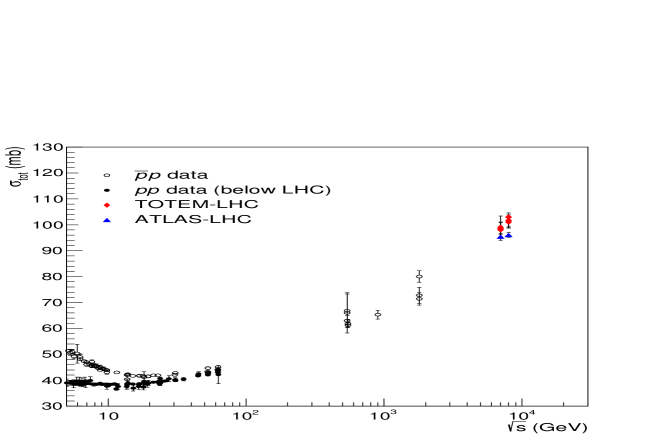
Figure 1: Total cross-section data from accelerator experiments on $pp$ (black circles, diamonds and triangles) and $\bar{p}p$ (white circles) collisions at the LHC energies and below (compiled from [54]).

A.2 Basic Phenomenological Concepts

As commented in our introduction, amplitude analyses, based on the $S$-Matrix formalism and Regge-Gribov theory [3, 11, 12], constitute the usual way to investigate the behavior of the total hadronic cross-section. In this context, the total cross-section is expressed as a sum of two terms, associated with Reggeons ($R$) and Pomerons ($P$) contributions.

$$\sigma_{tot}(s)=\sigma_{tot}^{R}(s)+\sigma_{tot}^{P}(s).$$ (25)

Detailed treatment can be found in the references quoted above and for a recent short review, see Appendix B in [25].

The essential idea of the formalism is to associate the asymptotic behavior of the scattering amplitude in terms of $s$ (named $s$-channel) with the singularities in the complex angular momentum plane $J$ (named $t$-channel), $s$ and $t$ being the Mandelstam variables. In this context, a simple pole located at $J=\alpha(t)$ (a Regge Pole),

$$\frac{1}{(J-\alpha(t))},$$

gives rise, for the asymptotic amplitude, to a power function of the energy [3, 11, 12, 25],

$$\mathrm{Im}\mathcal{A}(s,t)\propto s^{\alpha(t)}$$ (26)

and therefore, at $t=0$, for $\sigma_{tot}(s)$ through Eq. (1).

The connection with particle exchanged is interpreted as Reggeons ($R$) exchanges, associated with the highest interpolated mesonic trajectories provided by spectroscopic data ($t$-channel), relating Re$J=\alpha$ with the masses $M^{2}$ (the Chew-Frautschi plot) [3]. The trajectories are approximately linear,

$$\alpha(t)\approx\alpha_{0}+\alpha^{\prime}t,$$

defining an effective slope, $\alpha^{\prime}$, and an intercept, $\alpha_{0}$, which provides for $\sigma_{tot}$ ($t=0$) the exponent in the power law, negative and around 0.5 (Fig. 5.6 in [3]). In the 1960s, with experimental data available only in the region $\sqrt{s}<$ 20 GeV (see Fig. 1), these dependencies could explain the decrease of $\sigma_{tot}(s)$ as the energy increases. Taking account of the crossing symmetry and charge conjugation, these Reggeon contributions for $pp$ and $\bar{p}p$ scattering are expressed by

$$\sigma_{tot}^{R}(s) = a_{1}\left[\frac{s}{s_{0}}\right]^{-b_{1}}+\tau a_{2}\left[\frac{s}{s_{0}}\right]^{-b_{2}},$$ (27)

where $a_{i},b_{i},i=1,2$ are real positive parameters, $s_{0}$ is a fixed energy scale and $\tau=-1$ for $pp$ and $\tau=+1$ for $\bar{p}p$.

As new data have been obtained, new terms have been introduced. Firstly, the possibility that $\sigma_{tot}(s)$ decreased to a constant value (not zero) led to the introduction of a constant term, the Pomeranchuk constant or critical Pomeron (see [57] for historical fits with this contribution):

$$\sigma_{c}^{P}=A\ (\mathrm{constant}).$$ (28)

After the discovery of the rise of the total cross-section, above $\approx$ 20 GeV (Fig. 1), an ad hoc trajectory has been introduced with positive intercept $\alpha_{0}$ slightly greater than 1, named supercritical or soft Pomeron [3, 11], associated with a power law with exponent $\epsilon=\alpha_{0}-1$ slightly greater than 0:

$$\sigma_{sc}^{P}=s^{\epsilon}.$$ (29)

However, since this dependence eventually violates the FM bound, other forms have been studied, as logarithmic and/or logarithmic squared laws, which are associated with poles of higher order, double and triple poles, respectively, as we show in Sect. 2.2 and 3.1.

In the general case, associated with a pole of order $N$ ($t$-channel), the contribution to the forward amplitude in the $s$-channel is $s^{\alpha_{0}}\ln^{N-1}(s)$. In the case of the Pomeron, with a pole at $J=\alpha_{0}$ the contribution to the total cross-section is

$$\sigma^{P}_{tot}(s)=\frac{\mathrm{Im}\mathcal{A}(s,t=0)}{s}\propto s^{\alpha_{0}-1}\ln^{N-1}s.$$

Summarizing, we have the associations:

• simple pole ($N=1$) at $J=\alpha_{0}$, with $\alpha_{0}=1$  $\Rightarrow$  $\sigma^{P}_{tot}$  constant;

• simple pole ($N=1$) at $J=\alpha_{0}$  $\Rightarrow$  $\sigma^{P}_{tot}\propto s^{\alpha_{0}-1}$;

• double pole ($N=2$) at $J=\alpha_{0}$, with $\alpha_{0}=1$  $\Rightarrow$  $\sigma^{P}_{tot}\propto\ln(s)$;

• triple pole ($N=3$) at $J=\alpha_{0}$, with $\alpha_{0}=1$  $\Rightarrow$  $\sigma^{P}_{tot}\propto\ln^{2}(s)$.

A.3 Analytic parameterizations

A.3.1 RRPL2 Model

All the aforementioned different Pomeron contributions to $\sigma_{tot}(s)$ have been analyzed in detail by the COMPETE Collaboration in 2002, by means of simultaneous fits to $\sigma_{tot}$ and $\rho$ data (ratio between the real and imaginary parts of the forward amplitude), from several particle collisions ($pp$, $\bar{p}p$, mesons-$p$, $\gamma-p$, $\gamma-\gamma$). Analytic connections between $\sigma_{tot}$ and $\rho$ can be obtained in the context of the Regge theory (power laws) or mathematical approaches, such as dispersion relations or asymptotic uniqueness [25]. This study selected as the best model the one with the Pomeron ($P$) contribution expressed by a constant critical Pomeron term plus a log-squared contribution (triple pole) at the highest energies [13, 14]

$$\sigma^{P}_{tot}(s)=A+B\ln^{2}\left(\frac{s}{s_{0}}\right),$$ (30)

where $A$ and $B$ are free fit parameters. With the Reggeons contributions, Eq. (27), the analytic result is expressed by the sum of the contributions and is referred to as a RRPL2 model, standing for two Reggeons, Eq. (27), a constant Pomeranchuk term and a triple pole Pomeron term (L2), Eq. (30). This parametrization became a standard result in forward amplitude analyses and has been used and updated by the COMPAS group (IHEP, Protvino) in the successive editions of the Review of Particle Physics, by the PDG [15, 16].

A.3.2 RRPL$\gamma$ Model

In 1977 an empirical ansatz was introduced by Amaldi et al. [17] in the parametrization for $\sigma_{tot}$, represented by a log-raised-to-$\gamma$ (L$\gamma$), with $\gamma$ a free fit parameter, in place of the log-squared term (L2). From the above discussion, the full parametrization, recently denoted RRPL$\gamma$ in [24], is expressed by

$$\sigma_{tot}(s)=a_{1}\left[\frac{s}{s_{0}}\right]^{-b_{1}}+\tau a_{2}\left[\frac{s}{s_{0}}\right]^{-b_{2}}+A+B\ln^{\gamma}\left(\frac{s}{s_{0}}\right),$$ (31)

where $a_{i},b_{i},i=1,2$, $A$, $B$, $\gamma$ are free fit parameters, $s_{0}$ is a fixed energy scale and $\tau=-1$ for $pp$ and $\tau=+1$ for $\bar{p}p$.

In this case ($\gamma$ as a real parameter), the connections between $\sigma_{tot}$ and $\rho$ can be obtained either through numerical methods (integral dispersion relations) [17, 18, 19] or analytic methods: derivative dispersion relations (DDR) [20, 21, 22, 23, 24, 25] or asymptotic uniqueness (AU), which is based on the Phragmén-Lindelöff theorems [15, 16, 25]. All the analyses employing dispersion relations favour central values of $\gamma$ above 2 (in the interval 2.1 - 2.6, depending on the data then available and the kind of fit: only $\sigma_{tot}$ data or both $\sigma_{tot}$ and $\rho$ data). Contrasting with these results, analyses using the AU method favor $\gamma$-values slightly below 2 [15, 16] (see [25] for a detailed and comprehensive discussion on this subject). Anyway, all these analyses lead to good and consistent descriptions of the experimental data investigated. In the next Appendix, we illustrate the applicability of parametrization (31) to a particular case.

Appendix B Data Reductions to $pp$ and $\bar{p}p$ Total Cross-Sections

In this Appendix, in order to stress the practical importance of the exponent $\gamma$ as a real free parameter, we develop fits with the RRPL$\gamma$ model, Eq. (31), to the total cross-section data presently available at high energies (namely, above $\sqrt{s}$ = 5 GeV), shown in Fig. 1. For comparison, we shall also consider the particular case in which $\gamma=2$ is fixed, namely a RRPL2 model.

B.1 Fit Procedures and Results

As in our recent analysis [24, 25], we consider the energy scale fixed at the threshold for the scattering states, namely $s_{0}=4m_{p}^{2}=3.521$ GeV², where $m_{p}$ is the proton mass and we initialize our parametric set with the central values obtained in the most recent analyses by the PDG [16], also displayed in [24]. With these initial values, we first develop the fit with the RRPL2 model and using the final values as new feedbacks we develop the fit with the RRPL$\gamma$ model, namely by also letting free the parameter $\gamma$.

The data reductions were performed with the objects of the class TMinuit of ROOT Framework [58] and using the default MINUIT error analysis [59]. The error matrix provides the variances and covariances associated with each free parameter, which are used in the analytic evaluation of the uncertainty regions associated with the fitted and predicted quantities (through standard error propagation procedures [60]). As tests of goodness-of-fit we shall consider the chi-square per degree of freedom ($\chi^{2}/\nu$) and the corresponding integrated probability, $P(\chi^{2})$ [60].

The results of the fits are displayed in Table 1 (values of the free parameters with the uncertainties and statistical information) and Fig. 2. Although not taking part in the data reductions, we included in this figure, as illustration and for further reference, two estimations of the $pp$ total cross-section from cosmic-ray experiments, beyond the accelerator energy region: 57 TeV (Auger) [61] and 95 TeV (Telescope Array) [62]. The discrepancies between the TOTEM and ATLAS data (see Fig. 1) have been recently discussed in [24].

Table 1: Fit results to accelerator data on $pp$ and $\bar{p}p$ scattering above $\sqrt{s}$ = 5 GeV with models RRPL2 and RRPL$\gamma$, Eq. (31). Energy scale fixed, $s_{0}=4m_{p}^{2}=3.521$ GeV².

Model:	RRPL2	RRPL$\gamma$
$a_{1}$ (mb)	31.82 $\pm$ 0.70	31.2 $\pm$ 1.2
$b_{1}$	0.398 $\pm$ 0.017	0.500 $\pm$ 0.077
$a_{2}$ (mb)	16.72 $\pm$ 0.80	16.78 $\pm$ 0.84
$b_{2}$	0.539 $\pm$ 0.015	0.540 $\pm$ 0.016
$A$ (mb)	29.93 $\pm$ 0.35	33.3 $\pm$ 1.8
$B$ (mb)	0.2455 $\pm$ 0.0028	0.130 $\pm$ 0.055
$\gamma$	2 (fixed)	2.21 $\pm$ 0.14
$\nu$	168	167
$\chi^{2}/\nu$	1.02	1.01
$P(\chi^{2})$	0.420	0.457

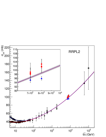
Figure 2: Fit results for the total cross-section, within the corresponding uncertainties regions, obtained through the RRPL2 and RRPL$\gamma$ models, Eq. (31), Table 1. The insert shows the $\sigma_{tot}$ data and curves in the interval 6 - 10 TeV (LHC region).

B.2 Discussion on the Fit Results

From Table 1, we see that the quality of the fit is good in both cases ($\chi^{2}/\nu\approx$ 1.0, for $\approx$ 170 degrees of freedom), with a result slightly better, as expected, in case of $\gamma$ as a free fit parameter: $P(\chi^{2})\approx$ 0.4 (RRPL2) and $P(\chi^{2})\approx$ 0.5 (RRPL$\gamma$).

Although the curves are very similar, note that differences appear as the energy increases above the accelerator data; indeed, the prediction with the RRPL2 model reaches the central value of the cosmic-ray point at 57 TeV (black square) and in case of the RRPL$\gamma$ model the prediction lies slightly above that central value, within the uncertainties. Once treated as a real free fit parameter, the value of $\gamma$ extracted from the fit, 2.21 $\pm$ 0.14, is consistent, within the uncertainties, with a rise of the total cross section faster than the log-squared dependence.

It is important to note that the leading high-energy component, expressed by

$$\sigma_{lead}=B\ln^{\gamma}(s/s_{0}),$$ (32)

provides also some interesting geometrical information. Indeed, in terms of the variable $\ln(s/s_{0})$, the rates of changes associated with the above leading component, namely slope ($S$) and curvature ($C$), are given by

$$S=B\gamma\ln^{\gamma-1}(s/s_{0}),\qquad C=B\gamma[\gamma-1]\ln^{\gamma-2}(s/s_{0}).$$ (33)

The RRPL2 model predicts constant curvature, $C_{L2}=2B$ and from Table 1, we obtain $C_{L2}\approx$ 0.49 mb. On the other hand, in case of $\gamma>2$, the curvature increases as the energy increases. From Table 1, $C_{L\gamma}\approx 0.3476\ln^{0.21}(s/3.521)$ mb. For example, for $\sqrt{s}=$ 10 TeV (typical of LHC region), we obtain $C_{L\gamma}\approx$ 0.63 mb.

We conclude that the data reduction with the RRPL$\gamma$ model does indicate a rise of the total cross-section faster than the log-squared dependence, as obtained in previous analyses restricted to total cross-section data [19, 20, 21, 22, 23] and suggested by some analyses including the $\rho$ data through dispersion relations [17, 18, 19, 21, 22, 23, 24, 25]. In other words, and for our purposes, these results disfavor a triple pole singularity (for which, $\gamma$ = 2).

References

- [1] F. Halzen and A.D. Martin, Quarks & Leptons: An Introductory Course in Modern Particle Physics, John Wiley & Sons, New York (1984).
- [2] W. Greiner, S. Schramm and E. Stein, Quantum Chromodynamics, 3rd edition Springer-Verlag, Berlin (2007).
- [3] V. Barone and E. Predazzi, High-Energy Particle Diffraction, Spring-Verlag, Berlin (2002).
- [4] M. Froissart, Asymptotic behavior and subtractions in the Mandelstam representation, Phys. Rev. 123, 1053 (1961).
- [5] A. Martin, Unitarity and high-energy behavior of scattering amplitudes, Phys. Rev. 129, 1432 (1963).
- [6] A. Martin, Extension of the axiomatic analyticity domain of scattering amplitudes by unitarity-I, Nuovo Cimento A 42, 930 (1966).
- [7] L. Lukaszuk and A. Martin, Absolute upper bounds for scattering, Nuovo Cimento A 52, 122 (1967).
- [8] Ya.I. Azimov, How robust is the Froissart bound?, Phys. Rev. D 84, 056012 (2011).
- [9] I.M. Dremin, Elastic scattering of hadrons, Phys. Usp. 56, 3 (2013).
- [10] G. Pancheri and Y.N. Srivastava, Introduction to the physics of the total cross-section at LHC: A review of data and models, Eur. Phys. J. C 77, 150 (2017).
- [11] S. Donnachie, G. Dosch, P.V. Landshoff and O. Natchmann, Pomeron Physics and QCD, Cambridge University Press, Cambridge (2002).
- [12] P.D.B. Collins, An Introduction to Regge Theory & High Energy Physics, Cambridge University Press, Cambridge (1977).
- [13] J.R. Cudell et al. (COMPETE Collaboration), Hadronic scattering amplitudes: Medium-energy constraints on asymptotic behavior, Phys. Rev. D 65, 074024 (2002).
- [14] J.R. Cudell et al. (COMPETE Collaboration), Benchmarks for the forward observables at RHIC, the Tevatron Run II and the LHC, Phys. Rev. Lett. 89, 201801 (2002).
- [15] K.A. Olive et al. (Particle Data Group), Review of Particle Physics, Chin. Phys. C 38, 090001 (2014).
- [16] C. Patrignani et al. (Particle Data Group), Review of Particle Physics, Chin. Phys. C 40, 100001 (2016).
- [17] U. Amaldi et al., The real part of the forward proton proton scattering amplitude measured at the CERN intersecting storage rings, Phys. Lett. B 66, 390 (1977).
- [18] C. Augier et al. (UA4/2 Collaboration), Predictions on the total cross-section and real part at LHC and SSC, Phys. Lett. B 315, 503 (1993).
- [19] A. Bueno and J. Velasco, A comparative study on two characteristic parameterizations for high energy and total cross-sections, Phys. Lett. B 380, 184 (1996).
- [20] D.A. Fagundes, M.J. Menon and P.V.R.G. Silva, Total hadronic cross-section data and the Froissart-Martin bound, Braz. J. Phys. 42, 452 (2012).
- [21] D.A. Fagundes, M.J. Menon and P.V.R.G. Silva, On the rise of proton-proton cross-sections at high energies, J. Phys. G 40, 065005 (2013).
- [22] M.J. Menon and P.V.R.G. Silva, An updated analysis on the rise of the hadronic total cross-section at the LHC energy region, Int. J. Mod. Phys. A 28, 1350099 (2013).
- [23] M.J. Menon and P.V.R.G. Silva, A study on analytic parameterizations for proton-proton cross-sections and asymptotia, J. Phys. G 40, 125001 (2013); J. Phys. G 41, 019501 (2014) [corrigendum].
- [24] D.A. Fagundes, M.J. Menon and P.V.R.G. Silva, Bounds on the rise of total cross-section from LHC7 and LHC8 data, Nucl. Phys. A 966, 185 (2017); e-Print: arXiv:1703.07486 [hep-ph],
- [25] D.A. Fagundes, M.J. Menon and P.V.R.G. Silva, Leading components in forward elastic hadron scattering: Derivative dispersion relations and asymptotic uniqueness, e-Print: arXiv:1705.01504 [hep-ph].
- [26] K.B. Oldham and J. Spanier, The Fraction Calculus-Theory and Applications of Differentiation and Integration to Arbitrary Order, Vol. 111 Mathematics in Science and Engineering, Ed. Bellman, R. Academic Press, San Diego (1999).
- [27] K.B. Oldham and J. Spanier, The Fractional Calculus, Dover, New York (2006).
- [28] R. Herrmann, Fractional Calculus: An Introduction for Physicists, World Scientific, New Jersey (2011).
- [29] H. Bateman, Tables of Integral Transforms, Volumes I & II (Bateman Manuscript Project), McGraw-Hill Book Company, New York (1954).
- [30] J. Bertrand, P. Bertrand, J. Ovarlez, “The Mellin Transform", The Transforms and Applications Handbook, 2nd edition, Ed. Alexander D. Poularikas. Boca Raton: CRC Press LLC (2000).
- [31] J. Oosthuizen, The Mellin Transform, http://math.sun.ac.za/wp-content/uploads/2013/02/Hons-Projek.pdf
- [32] M. Caputo, Linear models of dissipation whose Q is almost frequency independent - II, Geophys. J. Roy. Astron. Soc. 13, 529 (1967). Reprinted in Fract. Calc. App. Anal. 11, 4 (2008).
- [33] K. Diethelm, The Analysis of Fractional Differential Equations. An Application-Oriented Exposition Using Differential Operators of Caputo Type Lecture Notes in Mathematics, 204, Springer-Verlag Berlin Heidelberg (2010).
- [34] J. R. Forshaw, D. A. Ross, Quantum Chromodynamics and the Pomeron, Cambridge University Press, Cambridge (1997).
- [35] R. J. Eden, P. V. Landshoff, D. I. Olive, J. C. Polkinghorne, The Analytic S-Matrix, Cambridge University Press, Cambridge (1966).
- [36] R.J. Eden, High Energy Collisions of Elementary Particles, Cambridge University Press, Cambridge (1967).
- [37] I. S. Gradshteyn and I. M. Ryzhik, Table of Integrals, Series and Products, Academic Press, San Diego, CA (1980).
- [38] K. S. Miller and B. Ross, An Introduction to the Fractional Calculus and Fractional Differential Equations, Wiley, New York (1993).
- [39] B. Ross, (Ed.), Fractional Calculus and its Applications: Proceedings of the International Conference, New Haven, June 1974, Springer Verlag, New York (1974).
- [40] E. Capelas de Oliveira and J. A. Tenreiro Machado, A review of definitions for fractional derivatives and integral, Math. Prob. Ing. 2014, ID 238459 (2014).
- [41] K. Diethelm, The Analysis of Fractional Differential Equation, An Application-Oriented Exposition Using Differential Operators of Caputo Type, Springer, Springer-Verlag, Berlin-Heidelberg (2004).
- [42] F. Mainardi, Fractional Calculus and Waves in Linear Viscoelasticity, An Introduction to Mathematical Models, Imperial College Press, London (2010).
- [43] U. N. Katugampola, A new approach to generalized fractional derivatives, Bull. Math. Anal. Appl. 6, 1 (2014).
- [44] R. Khalil, M. al Horani, A. Yousef and M. Sababheh, A new definition of fractional derivative, J. Comput. & Appl. Math. 264, 65 (2014).
- [45] M. Caputo and M. Fabrizio, A new definition of fractional derivative without singular kernel, Prog. Fract. Differ. Appl. 1, 73 (2015).
- [46] J. Losada and J. J. Nieto, Properties of a new fractional derivative without singular kernel, Prog. Fract. Differ. Appl. 1, 87 (2015).
- [47] M. D. Ortigueira and J. A. Tenreiro Machado, What is a fractional derivative?, J. Comput. Phys. 293, 4 (2015).
- [48] B. Ross, A brief history and exposition of the fundamental theory of fractional calculus, in: B. Ross (Ed.), Fractional Calculus and its Applications, in: Lect. Notes Math., Springer-Verlag, Berlin, Heidelberg (1975), p. 1.
- [49] A. A. Kilbas, H. M. Srivastava, and J. J. Trujillo, Theory and Applications of Fractional Differential Equations, Elsevier, Amsterdam (2006).
- [50] D. S. Oliveira and E. Capelas de Oliveira, On a Caputo-type fractional derivative, submitted for publication (2017).
- [51] S. G. Samko, A. A. Kilbas and O. I. Marichev, Fractional Integrals and Derivatives: Theory and Applications, Gordon and Breach Science Publishers, Switzerland (1993).
- [52] J.R. Cudell, K. Kang and S.K. Kim, Bounds on the soft pomeron intercept, Phys. Lett. B 395, 311 (1997).
- [53] J.R. Cudell, A. Lengyel, E. Martynov and O.V. Selyugin, A review of the hard pomeron in soft diffraction, Nucl. Phys. A 755, 587 (2005).
- [54] http:// pdg.lbl.gov/2016/hadronic-xsections/hadron.html [16]. A complete list of data at the LHC energy-region and corresponding references can be found in [24], Table 1.
- [55] G. Antchev et al. (TOTEM Collaboration), Measurement of elastic pp scattering at 8 TeV in the Coulomb-nuclear interference region: determination of the parameter and the total cross-Section, Eur. Phys. J. C 76, 661 (2016).
- [56] M. Aaboud et al. (ATLAS Collaboration), Measurement of the total cross section from elastic scattering in pp collisions at = 8 TeV with the ATLAS detector, Phys. Lett. B 761, 158 (2016).
- [57] V. Barger, M. Olsson and D.D. Reeder, Asymptotic projections of scattering models, Nucl. Phys. B 5, 411 (1968).
- [58] ROOT Framework, http://root.cern.ch/drupal/; http://root.cern.ch/root/html/TMinuit.html
- [59] F. James, MINUIT Function Minimization and Error Analysis, Reference Manual, Version 94.1, CERN Program Library Long Writeup D506, CERN, Geneva, Switzerland (1998).
- [60] P. R. Bevington and D. K. Robinson, Data Reduction and Error Analysis for the Physical Sciences, 2nd ed., McGraw-Hill, Boston, Massachusetts (1992).
- [61] P. Abreu et al. (Pierre Auger Collaboration), Measurement of the proton-air cross-section at TeV with the Pierre Auger observatory, Phys. Rev. Lett. 109, 062002 (2012).
- [62] U. Abbasi et al. (Telescope Array Collaboration), Measurement of the proton-air cross-section with Telescope Array’s Middle Drum detector and surface array in hybrid mode, Phys. Rev. D 92, 032007 (2015); Erratum: Phys. Rev. D 92, 079901 (2015).