CTPU-17-28

KEK-TH-1990

Gravitational waves from first-order phase transitions:
Towards model separation by bubble nucleation rate

Ryusuke Jinno^a, Sangjun Lee^b,a,
Hyeonseok Seong^b and Masahiro Takimoto^c,d

a	Center for Theoretical Physics of the Universe, Institute for Basic Science (IBS),
	Daejeon 34051, Korea
b	Department of Physics, KAIST, Daejeon 34141, Korea,
c	Department of Particle Physics and Astrophysics, Weizmann Institute of Science,
	Rehovot 7610001, Israel
d	Theory Center, High Energy Accelerator Research Organization (KEK),
	Oho, Tsukuba, Ibaraki 305-0801, Japan

We study gravitational-wave production from bubble collisions in a cosmic first-order phase transition, focusing on the possibility of model separation by the bubble nucleation rate dependence of the resulting gravitational-wave spectrum. By using the method of relating the spectrum with the two-point correlator of the energy-momentum tensor $\left<T(x)T(y)\right>$, we first write down analytic expressions for the spectrum with a Gaussian correction to the commonly used nucleation rate, $\Gamma\propto e^{\beta t}\rightarrow e^{\beta t-\gamma^{2}t^{2}}$, under the thin-wall and envelope approximations. Then we quantitatively investigate how the spectrum changes with the size of the Gaussian correction. It is found that the spectral shape shows ${\mathcal{O}}(10)\%$ deviation from $\Gamma\propto e^{\beta t}$ case for some physically motivated scenarios. We also briefly discuss detector sensitivities required to distinguish different spectral shapes.

1 Introduction

Gravitational waves (GWs) offer the exciting possibility of probing the early Universe well before the Big Bang Nucleosynthesis and of revealing unknown high-energy particle physics. Possible cosmological sources of GWs include inflationary quantum fluctuations [1], preheating [2], topological defects [3] and first-order phase transitions [4, 5], and GWs from these sources are expected to be detected in the near future. In fact, ground-based GW detectors such as advanced LIGO [6], KAGRA [7] and VIRGO [8] are now in operation, and the first detections of GWs from black hole binaries by advanced LIGO collaboration [9, 10, 11] have opened up a new era of GW astronomy. In the future, space-borne detectors such as LISA [12], DECIGO [13] and BBO [14] are expected to start GW cosmology.

Among various sources of GWs in the early Universe, we focus on first-order phase transitions [4, 5] in this paper. Though first-order phase transitions do not occur in the standard model [15, 16, 17], there are various models which predict first-order phase transitions (see e.g. Refs. [25, 18, 19, 20, 24], and also Refs. [26, 27] and references therein for reviews). Furthermore, planned detectors are sensitive to the transition dynamics around TeV-PeV scales, and such GWs provide an opportunity of probing new physics beyond the standard model.

In thermal first-order phase transitions, bubbles of the true vacuum nucleate at some stage in the history of the Universe. They then expand because of the pressure difference between the true and false vacua, and the transition completes after they eventually collide with each other. Gravitational waves are produced during this process through their coupling to the energy-momentum tensor of the system. In other words, various properties of the energy-momentum tensor around the time of the high-energy transition are imprinted on the resulting GW spectrum. From the viewpoint of both knowing the dynamics in the early Universe and identifying the underlying particle physics, it is of great importance to study what kind of properties one may extract from the GW spectrum.

In first-order phase transitions, the main ingredients which determine the behavior of the energy-momentum tensor are classified as

• Spacetime distribution of bubbles (i.e., nucleation rate of bubbles),

• Energy-momentum tensor profile around a bubble wall,

• Dynamics after bubble collisions.

Much effort has been made to reveal the effects of (2) and (3) on the GW spectrum. For example, in the first numerical simulation of GW production in a vacuum transition (i.e., a system with only the scalar field which drives the transition) [28], it was found that the sourcing process is almost free from the detailed structure of the bubble walls. It was also found that the main GW production comes from the uncollided bubble walls. These findings led to “thin-wall” and “envelope” approximations, which were frequently used in subsequent works [29, 30, 31]: the former corresponds to assuming infinitely thin concentration of energy and momentum for (2), while the latter corresponds to assuming an instant damping of the wall energy and momentum for (3). Also, the authors of Refs. [32, 33, 34] have recently pointed out in a series of numerical simulations that in scalar-fluid systems the bulk motion of the fluid works as a long-lasting source for GWs (“sound waves”) even after bubbles collide with each other. This discovery has significantly changed our understanding on (3).

On the other hand, there are much less studies on the possibility of extracting information on (1) from the GW spectrum. However, in this paper we stress the importance of such studies because the spacetime distribution of bubbles is determined by the underlying particle physics through the time evolution of the bubble nucleation rate. In the literature the bubble nucleation rate in thermal first-order phase transitions has often been approximated simply by an exponential form $\Gamma\propto e^{\beta t}$. From the viewpoint of extracting as much information on the underlying particle physics as possible, we investigate the effect of the nucleation rate on the GW spectrum by going beyond the linear approximation $\Gamma\propto e^{\beta t}$.

For this purpose we adopt the method of relating the GW spectrum with the two-point ensemble average of the energy-momentum tensor $\left<T(x)T(y)\right>$. This method, which utilizes the stochastic nature of produced GWs, was first used in Ref. [42] in the context of bubble dynamics in first-order phase transitions. In Ref. [43] it has been pointed out that under the thin-wall approximation various contributions to this two-point correlator reduce to only two classes and the resulting spectrum becomes analytically calculable. As a result, the GW spectrum by the numerical simulation with the same setup in Ref. [44], i.e., the one with the thin-wall and envelope approximations, was derived analytically in Ref. [43]. This direction of study has recently been extended in Ref. [45], and a general form of the GW spectrum without the envelope approximation has been given and analyzed. In this paper, we focus on the effect of (1) on the GW spectrum. Therefore we adopt the simplest setup for (2) and (3): the thin-wall and envelope approximations. Though these approximations may not give a satisfactory description of the system, our study will give to some extent a quantitative measure of the dependence of the spectral shape on the nucleation rate.

The organization of the paper is as follows. In Sec. 2 we first make clear our assumptions and approximations on (1)–(3) above, and then present the formalism to calculate the GW spectrum. In Sec. 3 we give analytic expressions for the spectrum. In Sec. 4 we evaluate the expressions with numerical methods. Sec. 5 is devoted to conclusions. We also discuss typical models which realize deviations in the nucleation rate from the exponential form in Appendix A, and present a detailed derivation of the analytic expression of the spectrum in Appendix B. We briefly examine the asymptotic behavior of the spectrum in the limit of small Gaussian correction in Appendix C.

2 Formalism

In this section we first summarize the assumptions and approximations adopted in this paper, and then explain the method of relating the GW spectrum to the two-point correlator of the energy-momentum tensor $\left<T(x)T(y)\right>$.

2.1 Assumptions and approximations

Thin-wall and envelope approximations

First, we introduce two important approximations which determine (2) and (3): the thin-wall and envelope approximations. The former assumes that the energy released from the transition is localized around the thin surfaces of bubbles. We parameterize the energy-momentum tensor of an uncollided bubble as

$$T_{Bij}(x) =\rho_{B}(x)\widehat{(x-x_{n})}_{i}\widehat{(x-x_{n})}_{j},$$ (2.1)

where $x=(t_{x},\vec{x})$ denotes a spacetime point and $x_{n}=(t_{xn},\vec{x}_{n})$ is the nucleation point of the bubble. Also, $\hat{\bullet}$ denotes the unit vector in $\mathbf{\bullet}$ direction. In addition, we take $\rho_{B}$ to be

$$\rho_{B}(x) =\left\{\begin{array}[]{cc}\displaystyle\frac{4\pi}{3}r_{B}(t_{x},t_{xn})^{3}\kappa\rho_{0}\Big{/}4\pi r_{B}(t_{x},t_{xn})^{2}l_{B}&r_{B}(t_{x},t_{xn})<|\vec{x}-\vec{x}_{n}|<r^{\prime}_{B}(t_{x},t_{xn})\\ 0&{\rm otherwise}\end{array}\right.,$$ (2.4)

where $r_{B},r^{\prime}_{B}$ are the inner and outer radii of the bubble

$$r_{B}(t_{x},t_{xn}) =v(t_{x}-t_{xn}),\;\;\;r^{\prime}_{B}(t_{x},t_{xn})=r_{B}(t_{x},t_{xn})+l_{B}.$$ (2.5)

Here $l_{B}$ denotes the thickness of the wall, and we take $l_{B}\to 0$ in the final step. Also, $\rho_{0}$ is the released energy density, and the efficiency factor $\kappa$ determines the fraction of $\rho_{0}$ transformed into the macroscopic energy around the wall. In addition, $v$ is the wall velocity, which we assume to be constant throughout the paper. Note that the modeling (2.4) takes into account the proportionality of the released energy to the volume of the bubble and its localization within the bubble wall with width $l_{B}$. In the following calculations, we neglect the effect of cosmic expansion.

Nucleation rate

In this paper we parameterize the bubble nucleation as

$$\Gamma(t) =\Gamma_{*}e^{\beta t-\gamma^{2}t^{2}},$$ (2.6)

where $\beta$ and $\gamma$ are some constants and $\Gamma_{*}$ is the nucleation rate at some reference time, which we take to be $t=0$. Though $\gamma$ is often set to be zero in the literature, we aim to investigate the effect of this Gaussian correction on the spectral shape in this paper.

In the literature, the origin of time $t=0$ is often defined by the condition

$$\Gamma_{*} =H_{*}^{4},$$ (2.7)

where $H_{*}$ is the Hubble parameter at the time of transition. Note that in this paper we neglect the effect of cosmic expansion and thus $H_{*}$ is an input parameter. Though this definition completely specifies the form of the nucleation rate (2.6), it leads to redundancy among the parameters $(H_{*},\beta,\gamma)$ in presenting the GW spectrum. This is because of a time-shift invariance: $\Gamma(t)=\Gamma_{*}e^{\beta t-\gamma^{2}t^{2}}$ and $\Gamma(t)=\Gamma_{*}e^{\beta(t+\Delta t)-\gamma^{2}(t+\Delta t)^{2}}$ give the same GW spectrum for an arbitrary $\Delta t$ because the GW spectrum is obtained after integrating over the whole period of time. Therefore, in presenting the final results in Sec. 4, we eliminate this redundancy by choosing $\Delta t$ so that the nucleation rate is parameterized as

$$\Gamma(t) =\Gamma_{*}^{\prime}e^{\beta^{\prime}t^{\prime}-\gamma^{2}t^{\prime 2}},\;\;\;\;\Gamma_{*}^{\prime}=\beta^{\prime 4},\;\;\;\;t=t^{\prime}+\Delta t.$$ (2.8)

These new parameters satisfy

$$\frac{H_{*}^{4}}{\gamma^{4}}e^{\frac{\beta^{2}}{4\gamma^{2}}} =\frac{\beta^{\prime 4}}{\gamma^{4}}e^{\frac{\beta^{\prime 2}}{4\gamma^{2}}},$$ (2.11)

which should be regarded as an equation to determine $\gamma/\beta^{\prime}$ from the old parameters $\beta/H_{*}$ and $\gamma/\beta$. This new parameterization has a physical interpretation that $t^{\prime}=0$ corresponds to a typical transition time for $\beta^{\prime}/H_{*}\gg 1$ and $\gamma/\beta^{\prime}\ll 1$. Also, noting that the spectral shape is determined only by dimensionless quantities, we see that only $\gamma/\beta^{\prime}$ determines the spectral shape. In Fig. 1 we show the relation between $\gamma/\beta^{\prime}$ and $\gamma/\beta$ for several $\beta/H_{*}$.

In Table 1 we summarize several parameterizations of the nucleation rate obtained by the time shift. Parameterization 1 corresponds to the original one (2.6), while Parameterization 2 corresponds to the one introduced in Eq. (2.8). Also, we use Parameterization 3 when we introduce analytic expressions for the spectrum in Sec. 3 because it makes the expressions simplest. In presenting the final results in Sec. 4, we use Parameterization 2.

Finally, we mention typical values of $\beta^{\prime}/H_{*}$ and $\gamma/\beta^{\prime}$. The parameter $\beta^{\prime}/H_{*}$ largely depends on the particle physics setup and typically varies within $\sim\mathcal{O}{(10^{1-5})}$. On the other hand, the dependence of $\gamma/\beta^{\prime}$ on setups is relatively mild and it takes $\sim\mathcal{O}(0.1)$, though larger values are possible in very strong phase transitions [21, 22, 23, 40, 19, 24]. In Appendix A, we show that the typical value of $\gamma/\beta^{\prime}$ is $\mathcal{O}(0.1)$, and calculate it for some motivated models. Therefore, note that if we have $\mathcal{O}(0.1)$ sensitivity on $\gamma/\beta^{\prime}$ in future observations we have the possibility of distinguishing models by studying the spectral shape of GWs.

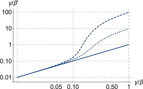
Figure 1: Relation (2.11) between dimensionless combinations $\gamma/\beta$ and $\gamma/\beta^{\prime}$. In this plot $\beta/H_{*}$ is taken to be $1,10,100$ from bottom to top.

Table 1: Equivalent parameterizations of the nucleation rate used in the paper.

Parameterization	1	2	3
Variables	$(\Gamma_{*},\beta,\gamma)$	$(\beta^{\prime},\gamma)$	$(\Gamma_{*}^{\prime\prime},\gamma)$
Nucleation rate $\Gamma$	$\Gamma_{*}e^{\beta t-\gamma^{2}t^{2}}$	$\Gamma_{*}^{\prime}e^{\beta^{\prime}t^{\prime}-\gamma^{2}t^{\prime 2}}$, $\Gamma_{*}^{\prime}=\beta^{\prime 4}$	$\Gamma_{*}^{\prime\prime}e^{-\gamma^{2}t^{\prime\prime 2}}$
Section	Sec. 2	Sec. 2, 3	Sec. 3, Appendix B

2.2 GW spectrum as energy-momentum tensor correlation

GW spectrum around the time of transition

As mentioned above, we neglect the effect of cosmic expansion during the transition. Under this approximation the metric is well described by

$$ds^{2} =-dt^{2}+(\delta_{ij}+2h_{ij})dx^{i}dx^{j}.$$ (2.12)

The evolution equation for the tensor perturbations $h_{ij}$ (satisfying the transverse and traceless conditions $h_{ii}=\partial_{i}h_{ij}=0$) is given by

$$\ddot{h}_{ij}(t,\vec{k})+k^{2}h_{ij}(t,\vec{k}) ={8\pi G}\Pi_{ij}(t,\vec{k}),$$ (2.13)

where the dot denotes the time derivative and we have moved to the Fourier space labeled by the three momentum $\vec{k}$. The source term $\Pi_{ij}$ denotes the projected energy-momentum tensor:

$$\Pi_{ij}(t,\vec{k}) =K_{ijkl}(\hat{k})T_{kl}(t,\vec{k}),$$ (2.14)

$$K_{ijkl}(\hat{k}) \equiv P_{ik}(\hat{k})P_{jl}(\hat{k})-\frac{1}{2}P_{ij}(\hat{k})P_{kl}(\hat{k}),\;\;\;\;P_{ij}(\hat{k})\equiv\delta_{ij}-\hat{k}_{i}\hat{k}_{j}.$$ (2.15)

We assume that the source is switched on from $t_{\rm start}$ to $t_{\rm end}$, which we take $t_{\rm start/end}\rightarrow\mp\infty$ in the following calculation.

The energy density of GWs is given by

$$\rho_{\rm GW}(t) =\frac{\langle\dot{h}_{ij}(t,\vec{x})\dot{h}_{ij}(t,\vec{x})\rangle}{8\pi G},$$ (2.16)

where the angular bracket denotes taking both an oscillation average for several oscillation periods and an ensemble average. In terms of the Fourier mode, the energy density per each logarithmic wavenumber is expressed as

$$\Omega_{\rm GW}(t,k) \equiv\frac{1}{\rho_{\rm tot}(t)}\frac{d\rho_{\rm GW}}{d\ln k}(t,k)=\frac{k^{3}}{16\pi^{3}G}P_{\dot{h}}(t,k).$$ (2.17)

Here we have normalized the energy density by the total energy density $\rho_{\rm tot}$ at time $t$ to define $\Omega_{\rm GW}$. Also, we have defined the power spectrum $P_{\dot{h}}$ as

$$\langle\dot{h}_{ij}(t,\vec{k})\dot{h}_{ij}^{*}(t,\vec{q})\rangle =(2\pi)^{3}\delta^{(3)}(\vec{k}-\vec{q})P_{\dot{h}}(t,k).$$ (2.18)

Since $h_{ij}$ is related to the source term $\Pi$ through Eq. (2.13), we can express $\Omega_{\rm GW}$ in terms of $\Pi$. For this purpose let us define the unequal-time correlator of the source term as

$$\langle\Pi_{ij}(t_{x},\vec{k})\Pi^{*}_{ij}(t_{y},\vec{q})\rangle =(2\pi)^{3}\delta^{(3)}(\vec{k}-\vec{q})\Pi(t_{x},t_{y},k).$$ (2.19)

This correlator is related to the original energy-momentum tensor through

$$\Pi(t_{x},t_{y},k) =K_{ijkl}(\hat{k})K_{ijmn}(\hat{k})\int d^{3}r\;e^{i\vec{k}\cdot\vec{r}}\langle T_{kl}T_{mn}\rangle(t_{x},t_{y},\vec{r}).$$ (2.20)

Here the quantity in the integrand is defined as

$$\langle T_{ij}T_{kl}\rangle(t_{x},t_{y},\vec{r}) \equiv\langle T_{ij}(t_{x},\vec{x})T_{kl}(t_{y},\vec{y})\rangle,$$ (2.21)

with $\vec{r}\equiv\vec{x}-\vec{y}$. Note that the spacial homogeneity of the system makes the correlator depend on $\vec{x}$ and $\vec{y}$ only through the combination $\vec{r}$. Now, using the Green function method, we obtain from Eq. (2.17) (see Refs. [42, 43, 45])

$$\Omega_{\rm GW}(t,k) =\frac{2Gk^{3}}{\pi\rho_{\rm tot}(t)}\int_{t_{\rm start}}^{t_{\rm end}}dt_{x}\int_{t_{\rm start}}^{t_{\rm end}}dt_{y}\;\cos(k(t_{x}-t_{y}))\Pi(t_{x},t_{y},k),\;\;\;\;t>t_{\rm end},$$ (2.22)

where we have assumed that the source term exists only from $t_{\rm start}$ to $t_{\rm end}$. This equation allows us to obtain the GW spectrum straightforwardly once we find expressions for $\Pi(t_{x},t_{y},k)$, or equivalently the two-point correlator $\langle T(x)T(y)\rangle$. Note that, though we have put the argument $t$, the L.H.S. essentially does not depend on it as long as $t>t_{\rm end}$ because there is no production or dilution of GWs once the source term is switched off.

We may further factor out some parameter dependences from Eq. (2.22). We first define the fraction of the released energy density to the background radiation energy density $\rho_{\rm rad}$ just before the transition as

$$\alpha \equiv\frac{\rho_{0}}{\rho_{\rm rad}},\;\;\;\;\;\;\rho_{\rm tot}=\rho_{0}+\rho_{\rm rad}.$$ (2.23)

Then, defining the dimensionless power spectrum $\Delta$ as

$$\Omega_{\rm GW}(t,k) \equiv\kappa^{2}\left(\frac{H_{*}}{\beta}\right)^{2}\left(\frac{\alpha}{1+\alpha}\right)^{2}\Delta(k/\beta),$$ (2.24)

we can factor out $G$, $\kappa$, $\rho_{0}$ and $\rho_{\rm tot}$ dependences. The new power spectrum $\Delta$ is expressed in terms of $\Pi$ as

$$\Delta(k/\beta) =\frac{3}{4\pi^{2}}\frac{\beta^{2}k^{3}}{\kappa^{2}\rho_{0}^{2}}\int_{t_{\rm start}}^{t_{\rm end}}dt_{x}\int_{t_{\rm start}}^{t_{\rm end}}dt_{y}\;\cos(k(t_{x}-t_{y}))\Pi(t_{x},t_{y},k),$$ (2.25)

where we have used the Friedmann equation $H_{*}^{2}=(8\pi G/3)\rho_{\rm tot}$. The spectrum $\Delta$ depends on dimensionless combinations such as $k/\beta$, $\gamma/\beta$ and $v$. Here we have kept only $k/\beta$ in the argument in order to make clear that $\Delta$ is a spectrum.

GW spectrum at present

Gravitational waves are redshifted after production until the present time. The present frequency $f_{0}$ and amplitude $\Omega_{{\rm GW},0}$ are obtained by taking into account that GWs behave as non-interacting radiation well inside the horizon (see Refs. [43, 45]):

$$f_{0} =1.65\times 10^{-5}{\rm Hz}\left(\frac{f_{*}}{\beta}\right)\left(\frac{\beta}{H_{*}}\right)\left(\frac{T_{*}}{10^{2}{\rm GeV}}\right)\left(\frac{g_{*}}{100}\right)^{\frac{1}{6}},$$ (2.26)

$$\Omega_{{\rm GW},0}(f_{0})h^{2} =1.67\times 10^{-5}\kappa^{2}\Delta(k/\beta)\left(\frac{H_{*}}{\beta}\right)^{2}\left(\frac{\alpha}{1+\alpha}\right)^{2}\left(\frac{g_{*}}{100}\right)^{-\frac{1}{3}},$$ (2.27)

where $g_{*}$ is the total number of relativistic degrees of freedom in the thermal bath at temperature $T_{*}$, and $f_{*}$ is the frequency at the time of transition. In Eq. (2.27), the present frequency $f_{0}$ is related to the wavenumber at the transition time $k$ through the relation (2.26) with $f_{*}=k/2\pi$. Note that the spectral shape is encoded in $\Delta$.

3 Analytic expressions

3.1 Basic strategy

We briefly summarize the basic strategy to calculate the GW spectrum. This subsection is essentially the same as Ref. [45]. From Eq. (2.25), we see that the spectrum is calculated from the unequal-time correlator $\Pi(t_{x},t_{y},k)$, which is the Fourier transform of $\Pi(t_{x},t_{y},\vec{r})$. Since the correlator $\Pi(t_{x},t_{y},\vec{r})$ is equivalent to $\left<T(t_{x},\vec{x})T(t_{y},\vec{y})\right>$ with $T$ symbolically denoting the energy-momentum tensor, the procedure we have to follow to obtain the spectrum is

• Fix the spacetime points $x=(t_{x},\vec{x})$ and $y=(t_{y},\vec{y})$.

• Find bubble configurations giving nonzero $T(x)T(y)$, calculate the probability for each configuration to occur, and estimate the value of $T(x)T(y)$ in each case.

• Sum over all possible configurations.

As in Refs. [43, 45], one may classify the bubble configurations depending on whether the contributions to $T(t_{x},\vec{x})$ and $T(t_{y},\vec{y})$ come from the same bubble or different bubbles. This consideration leads to the following classification:

• Single-bubble spectrum $\Delta^{(s)}$,

• Double-bubble spectrum $\Delta^{(d)}$.

The final spectrum $\Delta$ becomes the sum of the two: $\Delta=\Delta^{(s)}+\Delta^{(d)}$. Note that the single-bubble spectrum does not mean contributions from an isolated bubble (which would vanish) but it means that one sums over the configurations in which the wall fragments affecting $x$ and $y$ come from the same nucleation point (see Appendix H of Ref. [45] for more explanation).

3.2 Analytic expressions

Now we present analytic expressions for the single- and double-bubble spectrum. In order to make the final expressions as simple as possible, we shift the origin of time to eliminate the linear term in Eq. (2.6):

$$\Gamma(t) =\Gamma_{*}^{\prime\prime}e^{-\gamma^{2}t^{\prime\prime 2}},\;\;\;\;\Gamma_{*}^{\prime\prime}=\Gamma_{*}e^{\frac{\beta^{2}}{4\gamma^{2}}}=\beta^{\prime 4}e^{\frac{\beta^{\prime 2}}{4\gamma^{2}}},\;\;\;\;t^{\prime\prime}=t-\frac{\beta}{2\gamma^{2}}.$$ (3.1)

In the last two equations, we have presented relations to the other parameterizations. See Table 1. The spectral shape calculated from this parameterization has a dependence on the dimensionless combination $\Gamma_{*}^{\prime\prime}/\gamma^{4}$, which can be translated to a dependence on $\gamma/\beta^{\prime}$ through the second equation in Eq. (3.1).

Now, following the basic strategy illustrated in the previous subsection, we obtain (see Appendix B for the details of the derivation)

$$\Delta^{(s)} =\beta^{2}v^{6}k^{3}\;\Gamma_{*}^{\prime\prime}\int_{-\infty}^{\infty}dt^{\prime\prime}_{\left<x,y\right>}\int_{-\infty}^{\infty}dt^{\prime\prime}_{x,y}\int_{|t^{\prime\prime}_{x,y}|}^{\infty}dr_{v}$$

$$\;\;\;\;\;\;\;\;\;\;\;\;\;\;\;\;\;\;e^{-I(x,y)}\left[j_{0}(vkr_{v}){\mathcal{S}}_{0}+\frac{j_{1}(vkr_{v})}{vkr_{v}}{\mathcal{S}}_{1}+\frac{j_{2}(vkr_{v})}{(vkr_{v})^{2}}{\mathcal{S}}_{2}\right]\cos(kt^{\prime\prime}_{x,y}),$$ (3.2)

for the single-bubble spectrum and

$$\Delta^{(d)} =\beta^{2}v^{9}k^{3}\;\Gamma_{*}^{\prime\prime 2}\int_{-\infty}^{\infty}dt^{\prime\prime}_{\left<x,y\right>}\int_{-\infty}^{\infty}dt^{\prime\prime}_{x,y}\int_{|t^{\prime\prime}_{x,y}|}^{\infty}dr_{v}\;e^{-I(x,y)}\left[\frac{j_{2}(vkr_{v})}{(vkr_{v})^{2}}{\mathcal{D}}_{2}\right]\cos(kt^{\prime\prime}_{x,y}),$$ (3.3)

for the double-bubble spectrum. Here ${\mathcal{S}}_{0}$, ${\mathcal{S}}_{1}$, ${\mathcal{S}}_{2}$ and ${\mathcal{D}}_{2}$ are defined in Eqs. (B.15) and (B.25), and $j_{0}$, $j_{1}$ and $j_{2}$ are the spherical Bessel functions given by Eq. (B.13). Also, $I$ is given by Eq. (B.3).

We numerically checked that $\Delta^{(s)}(k)=\mathcal{O}(10^{0-1})\times\Delta^{(d)}(k)$ and $k_{\text{peak}}^{(s)}\simeq k_{\text{peak}}^{(d)}$ for $\gamma/\beta^{\prime}=10^{-1.0},\,10^{-0.5},\,10^{0.0},\,10^{0.5},\,10^{0.75}$ with $v=0.3,\,1.0$. It is a bit counter-intuitive that two contributions are in a similar order of magnitude. The spectrum depends on a correlator $\Pi(t_{x},t_{y},k)$ which is a Fourier transform of $\left<T(x)T(y)\right>$, and $\left<T(x)T(y)\right>$ is an integration of a probability times $T(x)T(y)$ for each configuration. A survival probability of the probability part is common, and in both “single-bubble” and “double-bubble” cases, the wall thickness $l_{B}$s are totally cancelled out. There are two factors making a difference. The first one is an extra factor $\Gamma^{\prime}_{*}r^{3}\Delta t=\beta^{\prime 4}r^{3}\Delta t\lesssim 1$ of a double-bubble case. $r$ is a representative radius of bubbles in the configuration, and $\Delta t$ is a time scale of consideration. The second one is an angular integration over nucleation points. Double-bubble nucleation points more destructively interfere with each other in the angular integration over nucleation points after the Fourier transform, thus it makes suppression. However, neither of the two suppressions is significant. They are expected to make $O(1)$ differences as numerical results show.

4 Numerical results

In this section we show the results for numerical evaluation of the spectrum (3.2) and (3.3). We have used a multi-dimensional integration algorithm VEGAS in the CUBA library [47]. In presenting the results, we define the spectrum normalized by its peak wavenumber $k_{\rm peak}$ and amplitude $\Delta_{\rm peak}$:

$$\tilde{\Delta}(\tilde{k}) \equiv\frac{\Delta(k)}{\Delta_{\rm peak}},\;\;\;\;\tilde{k}\equiv\frac{k}{k_{\rm peak}}.$$ (4.1)

By definition, $\tilde{\Delta}$ has its peak at $\tilde{k}=1$. This quantity makes it easier to compare the spectral shape. Also, since we would like to know the deviation of the spectral shape from the one with $\gamma=0$, we define the ratio $R(\tilde{k})$ between the normalized spectra $\tilde{\Delta}$ with $\gamma=0$ and $\gamma\neq 0$:

$$R(\tilde{k}) \equiv\frac{\tilde{\Delta}(\tilde{k})}{\tilde{\Delta}_{\gamma=0}(\tilde{k})}.$$ (4.2)

Here $\tilde{\Delta}_{\gamma=0}$ denotes the spectrum $\tilde{\Delta}$ with $\gamma=0$.

Now we present the results. First, we show the normalized total spectrum $\tilde{\Delta}$ for various values of $\gamma/\beta^{\prime}$ in Fig. 2. The wall velocity is taken to be $v=1$ (left) and $v=0.3$ (right), respectively. Observed features are

• The spectral shape starts to deviate from the one with $\gamma=0$ for $\gamma/\beta^{\prime}\sim{\mathcal{O}}(0.1)$.

• The spectral shape approaches to an asymptotic form for $\gamma/\beta^{\prime}\gg{\mathcal{O}}(0.1)$.

The latter behavior is because the setup reduces to the $\delta$-function nucleation rate $\Gamma(t)\propto\delta(t)$: see Appendix B.4 for details.

Next, we plot the ratio $R$ for $v=1$ and $v=0.3$ in Figs. 4 and 4, respectively. In these figures, the left panels show linear plots for the ratio $R$, while the right panels are logarithmic plots for the deviation $1-R$. The black shaded regions on the right panels represent the $0.1\%$ error coming from the cutoff for the Monte-Carlo integration. Observed features are

• For fixed $\gamma/\beta^{\prime}$, the deviation in the spectral shape (i.e. $1-R$) increases as $k$ deviates from $k_{\rm peak}$.

• The ratio $R$ approaches to constant in the small $k$ limit. On the other hand, we have not confirmed such behavior in the large $k$ limit due to numerical difficulties, though such a tendency is observed for example in Fig. 4 for large $\gamma/\beta^{\prime}$.

• For small $\gamma/\beta^{\prime}$, the values of $R$ in $v=1$ and $v=0.3$ cases show similar deviation from unity. For larger $\gamma/\beta^{\prime}$, however, the values of $R$ in $v=1$ case show a larger deviation from unity than $v=0.3$ case.

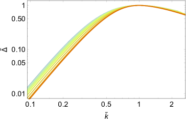
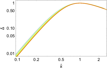
Figure 2: (Left) Spectral shape for $v=1$. (Right) Spectral shape for $v=0.3$.

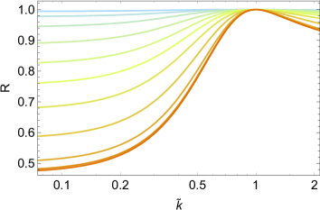
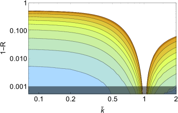
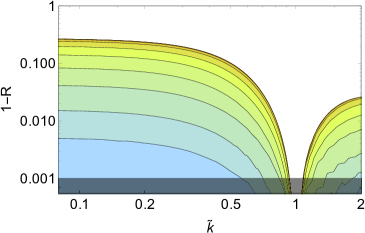
Figure 3: (Left) Ratio $R$ between the spectra with $\gamma=0$ and $\gamma\neq 0$ defined in Eq. (4.2). This figure shows $v=1$ case for various values of $\gamma/\beta^{\prime}$. (Right) Log plot of the left panel.

Figure 4: The same as Fig. 4 except that $v=0.3$.

Finally, let us briefly discuss the distinguishability of the spectral shape by future observations. We assume the detector sensitivity to be

$$\Omega_{\rm GW}^{\rm(det)}(f) =\Omega_{\rm GW,best}^{\rm(det)}\times\left\{\begin{matrix}\displaystyle\left(\frac{f}{f_{\rm best}}\right)^{-1}\;\;\;\;&(f<f_{\rm best}),\\ \displaystyle\left(\frac{f}{f_{\rm best}}\right)^{3}\;\;\;\;&(f>f_{\rm best}),\end{matrix}\right.$$ (4.3)

while we approximate the signal by

$$\Omega_{\rm GW}(f)=R\left(\frac{f}{f_{\rm peak}}\right)\times\Omega_{{\rm GW},\gamma=0}(f),$$ (4.4)

$$\Omega_{{\rm GW},\gamma=0}(f)=\Omega_{\rm GW,peak}\times\left\{\begin{matrix}\displaystyle\left(\frac{f}{f_{\rm peak}}\right)^{3}\;\;\;\;&(f<f_{\rm peak}),\\ \displaystyle\left(\frac{f}{f_{\rm peak}}\right)^{-1}\;\;\;\;&(f>f_{\rm peak}).\end{matrix}\right.$$ (4.5)

Here $f$ denotes the GW frequency, and the high and low frequency behavior of $\Omega_{\rm GW}^{\rm(det)}$ models the shot noise and the radiation pressure noise, respectively [48]. Note that the argument of $R$ satisfies $f/f_{\rm peak}=k/k_{\rm peak}$. We illustrate the setup in Fig. 6. In drawing the red-dashed line we have taken $v=1$ and extrapolated the ratio $R(f/f_{\rm peak})$ for $f/f_{\rm peak}<0.1$ and for $f/f_{\rm peak}>4$ by assuming that it is constant for these frequencies. Now let us define a condition for spectral shapes to be distinguished from each other by observations. We call the spectral shapes “distinguishable” if

$${}^{\exists}f\;\;\;:\;\;\;\Omega_{\rm GW}^{\rm(det)}(f)<\Delta\Omega_{\rm GW}(f)\equiv\Omega_{{\rm GW},\gamma=0}(f)-\Omega_{\rm GW}(f).$$ (4.6)

This means that, for fixed peak frequency and amplitude $(f_{\rm peak},\Omega_{\rm GW,peak})$, a detector with $(f_{\rm best},\Omega_{\rm GW,best}^{\rm(det)})$ can distinguish two spectral shapes with $\gamma\neq 0$ and $\gamma=0$. This is expected to give a rough estimate for the sensitivity to the value of $\gamma$.

Fig. 6 is a contour plot for $\gamma/\beta^{\prime}$ above which the distinguishable condition is satisfied. In this figure we have taken $v=1$ and varied $\gamma/\beta^{\prime}$ from $0.01$ to $5$. In making this figure, we have extrapolated the values of $R$ for $\gamma/\beta^{\prime}<0.1$ from $\gamma/\beta^{\prime}\geq 0.1$, due to numerical difficulties arising for small $\gamma/\beta^{\prime}$ (see Figs. 4–4). The extrapolation procedure is as follows. Regarding the Gaussian correction to the nucleation rate as a perturbation to the standard nucleation rate $\Gamma\propto e^{\beta t}$, one sees that the perturbation is controlled by $\gamma^{2}$. Noting that the spectral shape is affected only by dimensionless quantities, one expects that the deviation in the spectral shape from $\gamma=0$ case is proportional to $\gamma^{2}/\beta^{\prime 2}$ for small values of $\gamma/\beta^{\prime}$. We have confirmed this behavior at some fixed wavenumber, and we present the details in Appendix C. From this observation, we have extrapolated the values of $R$ by using $1-R\propto\gamma^{2}/\beta^{\prime 2}$ for small values of $\gamma/\beta^{\prime}$. In Fig. 6, it is shown that the spectral shape is distinguishable for $\Omega_{\rm GW,peak}/\Omega_{\rm GW,best}^{\rm(det)}\gtrsim{\mathcal{O}}(100)$ for moderate values $\gamma/\beta^{\prime}\sim{\mathcal{O}}(0.1)$.

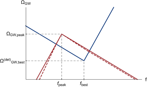
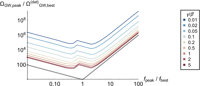
Figure 5: Setup in Eqs. (4.3)–(4.6). The blue line denotes the detector sensitivity curve (4.3), while the red lines correspond to the signal $\Omega_{{\rm GW},\gamma=0}$ (solid) and $\Omega_{\rm GW}$ with $\gamma/\beta^{\prime}=5$ (dashed). The bubble wall velocity is taken to be $v=1$, and we have extrapolated the normalized spectrum $R(f/f_{\rm peak})$ below $f/f_{\rm peak}<0.1$ and $f/f_{\rm peak}>4$ by assuming that it is constant for these frequencies. The extrapolation is expected to give conservative estimate for the deviation.

Figure 6: Contour plot of $\gamma/\beta^{\prime}$ above which the distinguishable condition (4.6) for the difference between the spectral shape with $\gamma\neq 0$ and $\gamma=0$ is satisfied. The detector sensitivity is given by Eq. (4.3), while the signal shape is given by Eq. (4.4). The wall velocity is taken to be $v=1$ and $\gamma/\beta^{\prime}$ is varied from $0.01$ (top) to $5$ (bottom). The gray line corresponds to the boundary where the condition ${}^{\exists}f$ : $\Omega_{\rm GW}^{\rm(det)}(f)=\Omega_{{\rm GW},\gamma=0}(f)$ is satisfied, i.e., detection of the spectrum with $\gamma=0$.

5 Conclusions

In this paper, we studied gravitational-wave (GW) production in the cosmic first-order phase transition. As stressed in Introduction, the GW spectrum resulting from the bubble dynamics contains information on

• Spacetime distribution of bubbles (i.e., nucleation rate of bubbles),

• Energy-momentum tensor profile around a bubble wall,

• Dynamics after bubble collisions.

In maximizing the amount of information on the unknown high-energy physics extracted from the spectrum, all these three aspects cannot be missed. In this paper we focused on the effect of (1) on the spectrum. For this purpose we used the method of relating the GW spectrum with the two-point ensemble average of the energy-momentum tensor $\left<T(x)T(y)\right>$. As pointed out in Ref. [43], all the contributions to this two-point correlator reduce to two classes under the thin-wall approximation (which refers to (2)). With the envelope approximation (which refers to (3)), we wrote down analytic expressions for the spectrum with the nucleation rate $\Gamma(t)\propto e^{\beta t-\gamma^{2}t^{2}}$, and investigated the effect of the Gaussian correction $\gamma$ on the spectrum.

As a result, we found that the spectral shape differs from the one without the Gaussian correction by ${\mathcal{O}}(10)\%$ for moderate values of $\gamma$ ($\gamma/\beta\sim{\mathcal{O}}(0.1))$, see Figs. 2–4. These values for the Gaussian correction are typically expected in various models as detailed in Appendix A. Therefore, as shown in Figs. 6–6, we have chances for extracting the information on the nucleation rate from the spectrum if the signal is well above the sensitivity of the GW detectors.

Model separation by the information encoded in the GW spectral shape is one of the most important tasks in this field. In this paper, we have shown that we can extract information about the Gaussian correction to the nucleation rate in a simplified setup. Though much remains to be done for model separation in a realistic setup, this direction will be worth investigating further in the future.

Appendix A Typical values of $\gamma/\beta^{\prime}$

In this appendix, we discuss typical values of the parameter $\gamma/\beta^{\prime}$. After discussing some general aspects, we estimate $\gamma/\beta^{\prime}$ for some motivated models. We will see that the typical value is around $\mathcal{O}(0.1)$  For notational simplicity, we write $\gamma/\beta^{\prime}$ as $\gamma/\beta$ in the following.

First, let us fix notations. In finite temperature field theory, the bubble nucleation rate per unit four volume is given by [51, 52]

$$\Gamma(T)=b(T)T^{4}e^{-S_{3}(T)/T},$$ (A.1)

where $S_{3}$ denotes the three dimensional bounce action and $b(T)\sim\mathcal{O}(1)$ denotes a contribution from the prefactor. Since the dependence of $\Gamma(T)$ on $b(T)$ is generically very weak compared to other dependences, we set $b(T)=1$. We rewrite the nucleation rate as

$$\Gamma(T) =M^{4}e^{-S(T)},$$ (A.2)

$$S(T) =\frac{S_{3}(T)}{T}-4\log(T/M),$$ (A.3)

where we have introduced some typical mass scale $M$ of a given model. At a given temperature $T$, we can relate $S(T)$ with $\beta$ and $\gamma$, which are expansion parameters of the nucleation rate in terms of time ($\Gamma(t)\propto e^{\beta t-\gamma^{2}t^{2}}$). By noticing $dT/dt=-HT$, we have

$$\frac{\beta}{H} =T\frac{dS(T)}{dT},$$ (A.4)

$$\frac{\gamma^{2}}{H^{2}} =\frac{1}{2}\left[\frac{\beta}{H}\left(1+\frac{T}{H}\frac{dH}{dT}\right)+T^{2}\frac{d^{2}S(T)}{dT^{2}}\right].$$ (A.5)

We use parameters $\beta/H$ and $\gamma/\beta$ instead of $\beta$ and $\gamma$ since they can be estimated only by the thermal field theory, that is, they can be calculated only from the bounce action $S(T)$ without the Einstein equation, as we see from Eqs. (A.4) and (A.5). As mentioned in Sec. 2.1, the phase transition mainly occurs when $\Gamma(T)\simeq\beta^{4}$. We define the transition temperature $T_{*}$ by the following condition

$$\Gamma(T_{*})=\beta(T_{*})^{4}.$$ (A.6)

We can rewrite this condition as follows:

$$S(T_{*})=4\log\left[\frac{M}{H(T_{*})}\right]+4\log\left[\frac{H(T_{*})}{\beta(T_{*})}\right].$$ (A.7)

For later convenience, we introduce $S_{C}(T)$ (with $C$ denoting “critical”) as

$$S_{C}(T)\equiv 4\log\left[\frac{M}{H(T)}\right]+4\log\left[\frac{H(T)}{\beta(T)}\right].$$ (A.8)

Now the transition condition, which determines $T_{*}$, is simply given by $S(T)=S_{C}(T)$.

Next, let us consider typical values of $\gamma/\beta$, which determine the spectral shape of GWs. Let us approximate the transition rate around the transition temperature by the following form

$$S=A(T+B)^{n},$$ (A.9)

with some constants $A$ and $B$ and $\mathcal{O}(1)$ constant $n$. When the derivative of the Hubble parameter in Eq. (A.5) is negligible, $\gamma/\beta$ at a given temperature $T$ is given by

$$\frac{\gamma}{\beta} =\sqrt{\frac{H}{2\beta}+\frac{n-1}{2n}\frac{1}{S(T)}}.$$ (A.10)

Since at the time of transition $\beta/H\sim 10^{1-5}$ and $S(T)\sim 100$ hold in most cases of interest, we expect $\gamma/\beta\sim\mathcal{O}(0.1)$ typically.

Below, we estimate $\gamma/\beta$ for some motivated models. We consider three models:

• Singlet extension of the standard model,

• Classically conformal $B-L$ model,

• Supersymmetric flaton model.

We will see that $\gamma/\beta\simeq 0.08$, $\gamma/\beta\simeq 0.1$ – $0.2$ and $\gamma/\beta\lesssim 0.04$ for the three cases, respectively. Thus, if we have $\mathcal{O}(0.1)$ sensitivity on $\gamma/\beta$, we can distinguish these models in principle.

A.1 Singlet extension of the standard model

First let us consider singlet extension of the standard model. Gravitational wave production in phase transitions in this type of model has been extensively studied in the literature. Here we consider a simplified version of this model. The potential is

$$V_{0} =-\frac{\mu^{2}}{2}h^{2}+\frac{\lambda_{H}}{4}h^{4}+\sum_{i=1}^{N_{s}}\left(\frac{m_{s}^{2}}{2}s_{i}^{2}+\frac{\lambda_{s}^{2}}{2}h^{2}s^{2}_{i}\right),$$ (A.11)

where $h$ represents the Higgs field, $s_{i}$ are real scalar fields and $N_{s}$ denotes the number of singlets. We take universal mass and coupling $m_{s}$ and $\lambda_{s}$ for these singlets. For the effective potential, we take only the one-loop part from singlet loops by assuming that these contributions dominate over those from the standard model. We have

$$V_{\rm 1-loop} =V_{\rm CW}+V_{\rm th},$$ (A.12)

where

$$V_{\rm CW}(h) =\frac{N_{S}(m_{s}^{2}+\lambda_{s}^{2}h^{2})^{2}}{64\pi^{2}}\log\left(\frac{m_{s}^{2}+\lambda_{s}^{2}h^{2}}{\Lambda^{2}}\right),$$ (A.13)

$$V_{\rm th}(h,T) =N_{S}V_{\rm th}^{B}(x,T),\;\;\;\;x\equiv\sqrt{m_{s}^{2}+\lambda_{s}^{2}h^{2}}/T,$$ (A.14)

$$V_{\rm th}^{B/F}(x,T) =\pm\frac{T^{4}}{2\pi^{2}}\int_{0}^{\infty}dz\;z^{2}\log\left[1\mp e^{-\sqrt{z^{2}+x^{2}}}\right],$$ (A.15)

where $V_{\rm CW}$ is the Coleman-Weinberg potential, $V_{\rm th}^{B/F}$ denotes thermal one-loop potential [53], and $\Lambda$ denotes the renormalization scale. Assuming $m^{2}_{s}\gtrsim\lambda_{s}^{2}T^{2}/6$, we neglect so-called daisy correction [54]. We fix the vacuum expectation value and mass of $h$ to those of the standard-model Higgs boson $v_{\rm EW}$ and $m_{H}$. For simplicity, we set $m_{s}^{2}/\lambda_{s}^{2}=v^{2}_{\rm EW}/6$ and $\Lambda^{2}=m_{s}^{2}+\lambda_{s}^{2}v_{\rm EW}^{2}$. Then, we have the following conditions:

$$\frac{\mu^{2}}{v_{\rm EW}^{2}} =\frac{1}{2}\frac{m_{H}^{2}}{v_{\rm EW}^{2}}-\frac{11}{192\pi^{2}}N_{s}\lambda_{s}^{4},$$ (A.16)

$$\lambda_{H} =\frac{1}{2}\frac{m_{H}^{2}}{v_{\rm EW}^{2}}-\frac{3}{32\pi^{2}}N_{s}\lambda_{s}^{4},$$ (A.17)

As a benchmark point, we take $N_{s}=10$, $\lambda_{s}=0.8$. Fig. 7 shows the temperature dependence of $S$, $S_{C}$, $\beta/H$ and $\gamma/\beta$. Here we have taken the typical mass scale to be $M=v_{\rm EW}$. The transition temperature $T_{*}$ is determined from $S(T_{*})=S_{C}(T_{*})$ as $T_{*}\simeq 0.6v_{\rm EW}$. At the transition temperature we have $\beta/H\simeq 4\times 10^{4}$ and $\gamma/\beta\simeq 0.08$.

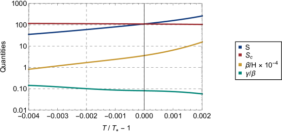
Figure 7: Temperature dependence of $S$, $S_{C}$, $\beta/H$ and $\gamma/\beta$ for the singlet extension model in Appendix A.1.

A.2 Classically conformal $B-L$ model

Next let us consider the classically conformal $B-L$ model [55, 56]. Gravitational wave production in such a scenario is considered in Refs. [18, 20]. In this model, we impose so-called “classical conformal invariance” based on the argument in Ref. [58], and also add U$(1)_{B-L}$ gauge symmetry. A complex scalar field $\Phi$ is introduced in order to break this U$(1)_{B-L}$ by its vacuum expectation value (VEV) and to induce the masses of the right handed neutrinos. The tree level scalar potential is given by

$$V=\lambda_{H}|H|^{4}+\lambda|\Phi|^{4}-\lambda^{\prime}|\Phi|^{2}|H|^{2},$$ (A.18)

where only quartic couplings appear due to the assumption of the classical conformal invariance. The VEV of the new field $M_{\Phi}\equiv\sqrt{2}\langle\Phi\rangle$ induces a negative mass term for the Higgs field and the electroweak scale can be realized. Below, we discuss a thermal phase transition of the $\Phi$ field.

For simplicity, we take $M_{\Phi}=10$ TeV $(\gg v_{\rm EW})$ and assume small right handed Yukawa couplings compered to the $B-L$ gauge coupling $g_{B-L}$. In such a case, the potential for $\Phi$ is mainly determined within $\Phi$ and $B-L$ gauge boson sector. The running of the quartic coupling $\lambda$ determines the potential for $\Phi$, and we can realize a minimum at $M_{\Phi}=10$ TeV. Now, because of the assumption $M_{\Phi}=10$ TeV, the only free parameter reduces the $B-L$ gauge coupling strength $\alpha_{B-L}(M_{\Phi})$ at scale $M_{\Phi}$.

Figure 9 shows the temperature dependence of $S$, $S_{C}$, $\beta/H$ and $\gamma/\beta$ for $\alpha_{B-L}(M_{\Phi})=0.01$. Here we have used the effective potential in Ref. [18] and taken the typical mass scale to be $M=M_{\Phi}$. The transition temperature is obtained as $T_{*}=5\times 10^{-3}M_{\Phi}$, and we have $\beta/H\simeq 20$ and $\gamma/\beta\simeq 0.12$ at this temperature. We also consider $\alpha_{B-L}(M_{\Phi})$ dependence of these parameters. Fig. 9 shows $\alpha_{B-L}(M_{\Phi})$ dependence of $\beta/H$ and $\gamma/H$ at the transition time. We see that the parameter $\gamma/\beta$ varies in a range $\gamma/\beta\simeq 0.1-0.2$.

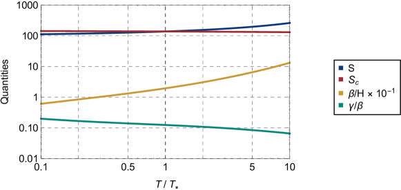
Figure 8: Temperature dependence of $S$, $S_{C}$, $\beta/H$ and $\gamma/\beta$ with $\alpha_{B-L}(M_{\Phi})=0.01$ for the classically conformal $B-L$ model.

Figure 9: $\alpha_{B-L}(M_{\Phi})$ dependence of $\beta/H$ and $\gamma/H$ at transition time for the classically conformal $B-L$ model.

A.3 Supersymmetric flaton model

Lastly we consider phase transitions after thermal inflation [59, 60] in supersymmetric flaton models. Gravitational wave production in such a scenario is studied in Ref. [61]. As in Ref. [61], we characterize the flaton potential by two parameters:

$$V(\phi)=V_{\rm TI}-\frac{1}{2}m_{\phi}^{2}\phi^{2}+\cdots,$$ (A.19)

where $m_{\phi}$ and $V_{\rm TI}$ denote the negative mass term and the potential energy around the origin, respectively. We assume that the potential shape is well approximated by this quadratic form for $\phi\lesssim m_{\phi}$. In addition, we assume that some higher-order terms stabilize the potential at $\phi\gg m_{\phi}$ and that we have $V(\langle\phi\rangle)=0$. In order to have a thermal potential, we add vector-like superfields $Q$ and $\bar{Q}$ with a superpotential

$$W\supset\lambda\Phi\bar{Q}Q.$$ (A.20)

As a benchmark model, we take $5$ and $\bar{5}$ representations of SU$(5)$ for $Q$ and $\bar{Q}$, respectively. In this case, the one-loop thermal potential is given by

$$\;\;\;\;\;\;\;\;V_{\rm th}=20V_{\rm th}^{B}(x,T)+20V_{\rm th}^{F}(y,T),$$ (A.21)

$$x\equiv\sqrt{m_{\phi}^{2}+\lambda^{2}\phi^{2}/2}/T,\;\;\;\;y\equiv\sqrt{\lambda^{2}\phi^{2}/2}/T,$$ (A.22)

where we have taken the mass of the scalar components of $Q$ and $\bar{Q}$ to be $m_{\phi}$, and neglected thermal masses for them.

Now we have three free parameters: the coupling $\lambda$, the mass scale $m_{\phi}$, and the size of the vacuum energy $V_{\rm TI}/m_{\phi}^{4}$. Fig. 11 shows the temperature dependence of $S$, $S_{C}$, $\beta/H$ and $\gamma/\beta$ for $\lambda=0.8$, $m_{\phi}=1$ TeV and $V_{\rm TI}/m_{\phi}^{4}=10^{4}$. Here we have taken the typical mass scale to be $M=m_{\phi}$. The transition temperature is given by $T_{*}\simeq 1.4m_{\phi}$, and we have $\beta/H\simeq 1500$ and $\gamma/\beta\simeq 0.04$ at the transition time. In this setup, the sign of $\gamma^{2}$ flips at a lower temperature. Fig. 11 shows the $V_{\rm TI}/m_{\phi}^{4}$ dependence of $\gamma/\beta$ at the transition time with $\lambda=0.8$ and $m_{\phi}=1$ TeV. We have $\beta/H\simeq 1000-2000$ for this region. We see that $\gamma/\beta$ decreases as $V_{\rm TI}/m_{\phi}^{4}$ increases. This is because the transition temperature $T_{*}$ becomes smaller for larger $V_{\rm TI}/m_{\phi}^{4}$: for larger $V_{\rm TI}/m_{\phi}^{4}$, $S_{C}$ becomes smaller because the Hubble parameter in the first term of Eq. (A.8) increases, and the transition temperature $T_{*}$ given by $S=S_{C}$ decreases. As a result, the sign of $\gamma^{2}$ at the transition time flips around $V_{\rm TI}/m_{\phi}^{4}\sim 10^{15}$. For the parameter values shown in this plot, $\gamma/\beta$ varies within $\gamma/\beta\lesssim 0.04$.

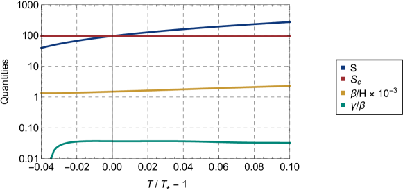
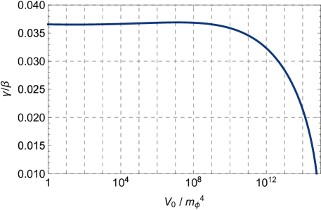
Figure 10: Temperature dependence of $S$, $S_{C}$, $\beta/H$ and $\gamma/\beta$ with $\lambda=0.8$, $V_{\rm TI}/m_{\phi}^{4}=10^{4}$ and $m_{\phi}=1$ TeV for the supersymmetric flaton model.

Figure 11: $V_{\rm TI}/m_{\phi}^{4}$ dependence of $\gamma/\beta$ at the transition time with $\lambda=0.8$ and $m_{\phi}=1$ TeV for the supersymmetric flaton model.

Appendix B Derivation of the analytic expressions

In this appendix we derive the analytic expressions (3.2) and (3.3). We use the nucleation rate shifted from the original form (2.6) so that the linear term vanishes:

$$\Gamma(t) =\Gamma_{*}^{\prime\prime}e^{-\gamma^{2}t^{\prime\prime 2}}.$$ (B.1)

In the following we take $\gamma=1$ unit. Also, in this appendix we simply write $\Gamma_{*}^{\prime\prime}$ and $t^{\prime\prime}$ as $\Gamma_{*}$ and $t$, respectively, for notational simplicity.

As mentioned in Sec. 3, what we need in order to obtain the GW spectrum is to calculate $\left<T(t_{x},\vec{x})T(t_{y},\vec{y})\right>$, with $x$ and $y$ denoting arbitrary four-dimensional spacetime points. In the thin-wall limit, there are two classes of contributions to $\left<T(t_{x},\vec{x})T(t_{y},\vec{y})\right>$, the single- and double-bubble, and thus the resulting GW spectrum can be classified into the single- and double-bubble spectra. In the derivation, we consider only those configurations with $r_{v}>|t_{x,y}|$ where $\vec{r}\equiv\vec{x}-\vec{y}$, $r\equiv|\vec{r}|$, $r_{v}\equiv r/v$ and $t_{x,y}\equiv t_{x}-t_{y}$ because only such configurations are relevant under the envelope approximation. First, we introduce the “false vacuum probability” $P(x,y)$, and then proceed to the calculation of the single- and double-bubble spectra. We follow the notation of Appendix A in Ref. [45].

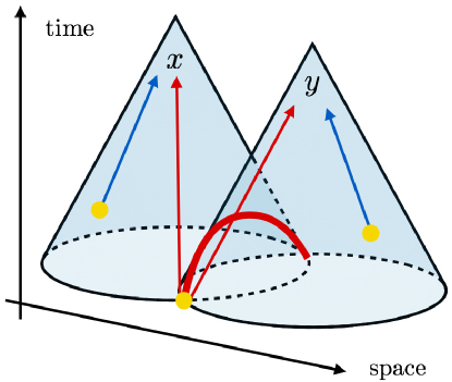
Figure 12: 3-dimensional plot of the paths of the bubble wall fragments of $x$ and $y$. These bubbles nucleate on the surfaces of the past $v$-cones of $x$ and $y$. Bubble wall propagation in the single- and double-bubble contributions is shown as red and blue lines, respectively. The same figure as in Refs. [43, 45].

B.1 False vacuum probability

Let us consider the probability $P(x,y)$ with which both of the spacetime points $x$ and $y$ remain in the false vacuum. It is equivalent to the probability for no bubbles to nucleate in $V_{xy}\equiv V_{x}\cup V_{y}$, where $V_{x}$ and $V_{y}$ are the regions inside the past $v$-cones (past cones with velocity $v$) of $x$ and $y$, respectively (see Fig. 12). Then, the probability is given by

$$P(x,y) =e^{-I(x,y)},\;\;\;\;I(x,y)=\int_{V_{xy}}d^{4}z\;\Gamma(z).$$ (B.2)

Let us write down an explicit form of the function $I$. The spacial volume of $V_{xy}$ on the constant-time hypersurface $\Sigma_{t}$ at time $t$ consists of intersecting spheres for $t<t_{\rm max}$, but separate sphere(s) for $t>t_{\rm max}$, where $t_{\rm max}\equiv(t_{x}+t_{y}-r_{v})/2$. Note that $t_{\rm max}$ is the latest time when two past $v$-cones intersect with each other in Fig. 12. Then $I$ is given by

$$I(x,y) =\int_{-\infty}^{t_{\rm max}}dt\;\Gamma(t)\left[\frac{\pi}{3}r_{x}^{3}(2+c_{\times x})(1-c_{\times x})^{2}+\frac{\pi}{3}r_{y}^{3}(2-c_{\times y})(1+c_{\times y})^{2}\right]$$

$$\;\;\;\;+\int_{t_{\rm max}}^{t_{x}}dt\;\Gamma(t)\frac{4\pi}{3}r_{x}^{3}+\int_{t_{\rm max}}^{t_{y}}dt\;\Gamma(t)\frac{4\pi}{3}r_{y}^{3}.$$ (B.3)

Here $r_{x}$ and $r_{y}$ are defined as $r_{x}\equiv v(t_{x}-t)$ and $r_{y}\equiv v(t_{y}-t)$, respectively, and the cosines have relations

$$c_{\times x} =-\frac{r_{x}^{2}+r^{2}-r_{y}^{2}}{2r_{x}r},\;\;\;\;c_{\times y}=\frac{r_{y}^{2}+r^{2}-r_{x}^{2}}{2r_{y}r}.$$ (B.4)

Note that the quantity in the squared parenthesis in Eq. (B.3) is the spacial volume of $V_{xy}$ on $\Sigma_{t}$ for $t<t_{\rm max}$. Given the nucleation rate (B.1), it is straightforward to evaluate this integral. We obtain

$$I(x,y) =v^{3}\Gamma_{*}\left(\begin{matrix}c_{{\rm Exp},t_{x,y}}\\ c_{{\rm Exp},-t_{x,y}}\\ c_{{\rm Exp},-r_{v}}\\ c_{1+{\rm Erf},t_{x,y}}\\ c_{1+{\rm Erf},-t_{x,y}}\\ c_{1+{\rm Erf},-r_{v}}\end{matrix}\right)^{\rm T}\left(\begin{matrix}\displaystyle{\rm Exp}\left[-\left(t_{\left<x,y\right>}+\frac{t_{x,y}}{2}\right)^{2}\right]\\ \displaystyle{\rm Exp}\left[-\left(t_{\left<x,y\right>}-\frac{t_{x,y}}{2}\right)^{2}\right]\\ \displaystyle{\rm Exp}\left[-\left(t_{\left<x,y\right>}-\frac{r_{v}}{2}\right)^{2}\right]\\ \displaystyle 1+{\rm Erf}\left[t_{\left<x,y\right>}+\frac{t_{x,y}}{2}\right]\\ \displaystyle 1+{\rm Erf}\left[t_{\left<x,y\right>}-\frac{t_{x,y}}{2}\right]\\ \displaystyle 1+{\rm Erf}\left[t_{\left<x,y\right>}-\frac{r_{v}}{2}\right]\end{matrix}\right),$$ (B.5)

where $t_{\left<x,y\right>}\equiv(t_{x}+t_{y})/2$ and “T” denotes the transpose. The coefficients are given by

$$c_{{\rm Exp},t_{x,y}}=\frac{\pi}{6}\left(\begin{matrix}1\\ t_{\left<x,y\right>}\\ t_{\left<x,y\right>}^{2}\end{matrix}\right)^{\rm T}\left(\begin{matrix}4&0&1\\ 0&4&0\\ 4&0&0\end{matrix}\right)\left(\begin{matrix}1\\ t_{x,y}\\ t_{x,y}^{2}\end{matrix}\right),$$ (B.6)

$$c_{{\rm Exp},-t_{x,y}}=\frac{\pi}{6}\left(\begin{matrix}1\\ t_{\left<x,y\right>}\\ t_{\left<x,y\right>}^{2}\end{matrix}\right)^{\rm T}\left(\begin{matrix}4&0&1\\ 0&-4&0\\ 4&0&0\end{matrix}\right)\left(\begin{matrix}1\\ t_{x,y}\\ t_{x,y}^{2}\end{matrix}\right),$$ (B.7)

$$c_{{\rm Exp},-r_{v}}=\frac{\pi}{24}\frac{1}{r_{v}}\left(\begin{matrix}1\\ t_{\left<x,y\right>}\\ t_{\left<x,y\right>}^{2}\end{matrix}\right)^{\rm T}\left(\begin{matrix}-16r_{v}+2r_{v}^{3}&0&-6r_{v}\\ 4r_{v}^{2}&0&12\\ -16r_{v}&0&0\end{matrix}\right)\left(\begin{matrix}1\\ t_{x,y}\\ t_{x,y}^{2}\end{matrix}\right),$$ (B.8)

$$c_{1+{\rm Erf},t_{x,y}}=\frac{\pi^{3/2}}{12}\left(\begin{matrix}1\\ t_{\left<x,y\right>}\\ t_{\left<x,y\right>}^{2}\\ t_{\left<x,y\right>}^{3}\end{matrix}\right)^{\rm T}\left(\begin{matrix}0&6&0&1\\ 12&0&6&0\\ 0&12&0&0\\ 8&0&0&0\end{matrix}\right)\left(\begin{matrix}1\\ t_{x,y}\\ t_{x,y}^{2}\\ t_{x,y}^{3}\end{matrix}\right),$$ (B.9)

$$c_{1+{\rm Erf},-t_{x,y}}=\frac{\pi^{3/2}}{12}\left(\begin{matrix}1\\ t_{\left<x,y\right>}\\ t_{\left<x,y\right>}^{2}\\ t_{\left<x,y\right>}^{3}\end{matrix}\right)^{\rm T}\left(\begin{matrix}0&-6&0&-1\\ 12&0&6&0\\ 0&-12&0&0\\ 8&0&0&0\end{matrix}\right)\left(\begin{matrix}1\\ t_{x,y}\\ t_{x,y}^{2}\\ t_{x,y}^{3}\end{matrix}\right),$$ (B.10)

$$c_{1+{\rm Erf},-r_{v}}=\frac{\pi^{3/2}}{24}\frac{1}{r_{v}}\left(\begin{matrix}1\\ t_{\left<x,y\right>}\\ t_{\left<x,y\right>}^{2}\\ t_{\left<x,y\right>}^{3}\end{matrix}\right)^{\rm T}\left(\begin{matrix}6r_{v}^{2}-r_{v}^{4}&0&6+3r_{v}^{2}\\ -24r_{v}&0&-12r_{v}\\ 12r_{v}^{2}&0&12\\ -16r_{v}&0&0\end{matrix}\right)\left(\begin{matrix}1\\ t_{x,y}\\ t_{x,y}^{2}\end{matrix}\right).$$ (B.11)

B.2 Single-bubble spectrum

Let us now derive the single-bubble spectrum. In the thin-wall limit, the necessary and sufficient conditions for the wall of a single bubble to contribute to the energy-momentum tensor at both of the spacetime points $x$ and $y$ are summarized as

• No bubble nucleates in $V_{xy}$.

• One bubble nucleates in $\delta V_{xy}$.

Here $\delta V_{xy}$, shown as the red line in Fig. 12, is the narrow four-dimensional region on the two past $v$-cones: $\delta V_{xy}\equiv(V_{x+\delta}-V_{x})\cap(V_{y+\delta}-V_{y})$ with $x+\delta\equiv(t_{x}+l_{B}/v,\vec{x})$ and $y+\delta\equiv(t_{y}+l_{B}/v,\vec{y})$. Following the same procedure as in Appendix A in Ref. [45], we obtain

$$\Pi^{(s)}(t_{x},t_{y},k)$$

$$=\frac{4\pi^{2}}{9}\kappa^{2}\rho_{0}^{2}\int_{v|t_{x,y}|}^{\infty}dr\int_{-\infty}^{t_{\rm max}}dt_{n}\;e^{-I(x,y)}\Gamma(t_{n})\;rr_{x}^{(s)2}r_{y}^{(s)2}\left[j_{0}(kr){\mathcal{K}}_{\times 0}+\frac{j_{1}(kr)}{kr}{\mathcal{K}}_{\times 1}+\frac{j_{2}(kr)}{(kr)^{2}}{\mathcal{K}}_{\times 2}\right].$$ (B.12)

Here $t_{n}$ denotes the nucleation time of the bubble nucleated in $\delta V_{xy}$. See Ref. [45] for the definition of the other quantities. In Eq. (B.12), all the $l_{B}$’s have been canceled out because the allowed volume for bubble nucleation (the thick red line in Fig. 12) is proportional to $l_{B}^{2}$ while the resulting $T(x)T(y)$ is proportional to $l_{B}^{-2}$. Also, $j_{0}$, $j_{1}$ and $j_{2}$ are the spherical Bessel functions defined as

$$j_{0}(x) =\frac{\sin x}{x},\;\;\;\;j_{1}(x)=\frac{\sin x-x\cos x}{x^{2}},\;\;\;\;j_{2}(x)=\frac{(3-x^{2})\sin x-3x\cos x}{x^{3}}.$$ (B.13)

After integrating out the nucleation time, we obtain

$$\Pi^{(s)}(t_{x},t_{y},k) =\frac{4\pi^{2}}{3}v^{6}\kappa^{2}\rho_{0}^{2}\;\Gamma_{*}\int_{|t_{x,y}|}^{\infty}dr_{v}\;e^{-I(x,y)}\left[j_{0}(vkr_{v}){\mathcal{S}}_{0}+\frac{j_{1}(vkr_{v})}{vkr_{v}}{\mathcal{S}}_{1}+\frac{j_{2}(vkr_{v})}{(vkr_{v})^{2}}{\mathcal{S}}_{2}\right],$$ (B.14)

where ${\mathcal{S}}_{0}$, ${\mathcal{S}}_{1}$ and ${\mathcal{S}}_{2}$ are given by

$${\mathcal{S}}_{0} =c_{{\rm Exp},0}^{(s)}{\rm Exp}\left[-\left(t_{\left<x,y\right>}-\frac{r_{v}}{2}\right)^{2}\right]+c_{1+{\rm Erf},0}^{(s)}\left(1+{\rm Erf}\left[t_{\left<x,y\right>}-\frac{r_{v}}{2}\right]\right),$$

$${\mathcal{S}}_{1} =c_{{\rm Exp},1}^{(s)}{\rm Exp}\left[-\left(t_{\left<x,y\right>}-\frac{r_{v}}{2}\right)^{2}\right]+c_{1+{\rm Erf},1}^{(s)}\left(1+{\rm Erf}\left[t_{\left<x,y\right>}-\frac{r_{v}}{2}\right]\right),$$

$${\mathcal{S}}_{2} =c_{{\rm Exp},2}^{(s)}{\rm Exp}\left[-\left(t_{\left<x,y\right>}-\frac{r_{v}}{2}\right)^{2}\right]+c_{1+{\rm Erf},2}^{(s)}\left(1+{\rm Erf}\left[t_{\left<x,y\right>}-\frac{r_{v}}{2}\right]\right),$$ (B.15)

with the coefficients

$$c_{{\rm Exp},0}^{(s)}=\frac{1}{96}\frac{(t_{x,y}^{2}-r_{v}^{2})^{2}}{r_{v}^{3}}\left(\begin{matrix}1\\ t_{\left<x,y\right>}\\ t_{\left<x,y\right>}^{2}\\ t_{\left<x,y\right>}^{3}\end{matrix}\right)^{\rm T}\left(\begin{matrix}12r_{v}-2r_{v}^{3}\\ 40-4r_{v}^{2}\\ 8r_{v}\\ 16\end{matrix}\right),$$ (B.16)

$$c_{1+{\rm Erf},0}^{(s)}=\frac{\sqrt{\pi}}{96}\frac{(t_{x,y}^{2}-r_{v}^{2})^{2}}{r_{v}^{3}}\left(\begin{matrix}1\\ t_{\left<x,y\right>}\\ t_{\left<x,y\right>}^{2}\\ t_{\left<x,y\right>}^{3}\\ t_{\left<x,y\right>}^{4}\end{matrix}\right)^{\rm T}\left(\begin{matrix}12-4r_{v}^{2}+r_{v}^{4}\\ 0\\ 48-8r_{v}^{2}\\ 0\\ 16\end{matrix}\right),$$ (B.17)

$$c_{{\rm Exp},1}^{(s)}=\frac{1}{96}\frac{t_{x,y}^{2}-r_{v}^{2}}{r_{v}^{3}}\left(\begin{matrix}1\\ t_{\left<x,y\right>}\\ t_{\left<x,y\right>}^{2}\\ t_{\left<x,y\right>}^{3}\end{matrix}\right)^{\rm T}\left(\begin{matrix}24r_{v}^{3}+12r_{v}^{5}&0&-120r_{v}+4r_{v}^{3}\\ 80r_{v}^{2}+24r_{v}^{4}&0&-400+8r_{v}^{2}\\ 16r_{v}^{3}&0&-80r_{v}\\ 32r_{v}^{2}&0&-160\end{matrix}\right)\left(\begin{matrix}1\\ t_{x,y}\\ t_{x,y}^{2}\end{matrix}\right),$$ (B.18)

$$c_{1+{\rm Erf},1}^{(s)}=\frac{\sqrt{\pi}}{96}\frac{t_{x,y}^{2}-r_{v}^{2}}{r_{v}^{3}}\left(\begin{matrix}1\\ t_{\left<x,y\right>}\\ t_{\left<x,y\right>}^{2}\\ t_{\left<x,y\right>}^{3}\\ t_{\left<x,y\right>}^{4}\end{matrix}\right)^{\rm T}\left(\begin{matrix}24r_{v}^{2}+8r_{v}^{4}-6r_{v}^{6}&0&-120+24r_{v}^{2}-2r_{v}^{4}\\ 0&0&0\\ 96r_{v}^{2}+16r_{v}^{4}&0&-480+48r_{v}^{2}\\ 0&0&0\\ 32r_{v}^{2}&0&-160\end{matrix}\right)\left(\begin{matrix}1\\ t_{x,y}\\ t_{x,y}^{2}\end{matrix}\right),$$ (B.19)

$$c_{{\rm Exp},2}^{(s)}=\frac{1}{96}\frac{1}{r_{v}^{3}}\left(\begin{matrix}1\\ t_{\left<x,y\right>}\\ t_{\left<x,y\right>}^{2}\\ t_{\left<x,y\right>}^{3}\end{matrix}\right)^{\rm T}\left(\begin{matrix}36r_{v}^{5}+10r_{v}^{7}&0&-360r_{v}^{3}-36r_{v}^{5}&0&420r_{v}+10r_{v}^{3}\\ 120r_{v}^{4}+20r_{v}^{6}&0&-1200r_{v}^{2}-72r_{v}^{4}&0&1400+20r_{v}^{2}\\ 24r_{v}^{5}&0&-240r_{v}^{3}&0&280r_{v}\\ 48r_{v}^{4}&0&-480r_{v}^{2}&0&560\end{matrix}\right)\left(\begin{matrix}1\\ t_{x,y}\\ t_{x,y}^{2}\\ t_{x,y}^{3}\\ t_{x,y}^{4}\end{matrix}\right),$$ (B.20)

$$c_{1+{\rm Erf},2}^{(s)}=\frac{\sqrt{\pi}}{96}\frac{1}{r_{v}^{3}}$$

$$\times\left(\begin{matrix}1\\ t_{\left<x,y\right>}\\ t_{\left<x,y\right>}^{2}\\ t_{\left<x,y\right>}^{3}\\ t_{\left<x,y\right>}^{4}\end{matrix}\right)^{\rm T}\left(\begin{matrix}36r_{v}^{4}+4r_{v}^{6}+3r_{v}^{8}&0&-360r_{v}^{2}+24r_{v}^{4}+2r_{v}^{6}&0&420-60r_{v}^{2}+3r_{v}^{4}\\ 0&0&0&0&0\\ 144r_{v}^{4}+8r_{v}^{6}&0&-1440r_{v}^{2}+48r_{v}^{4}&0&1680-120r_{v}^{2}\\ 0&0&0&0&0\\ 48r_{v}^{4}&0&-480r_{v}^{2}&0&560\end{matrix}\right)\left(\begin{matrix}1\\ t_{x,y}\\ t_{x,y}^{2}\\ t_{x,y}^{3}\\ t_{x,y}^{4}\end{matrix}\right).$$ (B.21)

Then, the single-bubble spectrum is obtained by using Eq. (2.25):

$$\Delta^{(s)}=\beta^{2}v^{6}k^{3}\;\Gamma_{*} \int_{-\infty}^{\infty}dt_{\left<x,y\right>}\int_{-\infty}^{\infty}dt_{x,y}\int_{|t_{x,y}|}^{\infty}dr_{v}$$

$$e^{-I(x,y)}\left[j_{0}(vkr_{v}){\mathcal{S}}_{0}+\frac{j_{1}(vkr_{v})}{vkr_{v}}{\mathcal{S}}_{1}+\frac{j_{2}(vkr_{v})}{(vkr_{v})^{2}}{\mathcal{S}}_{2}\right]\cos(kt_{x,y}).$$ (B.22)

B.3 Double-bubble spectrum

Next let us derive the double-bubble spectrum. The necessary and sufficient conditions for the walls of two different bubbles to contribute to the energy-momentum tensor at $x$ and $y$ are summarized as

• No bubble nucleates in $V_{xy}$.

• One bubble nucleates in $\delta V_{x}^{(y)}$, and another nucleates in $\delta V_{y}^{(x)}$.

Here $\delta V_{x}^{(y)}$ and $\delta V_{y}^{(x)}$ are thin surfaces of $V_{x}$ and $V_{y}$ in Fig. 12: $\delta V_{x}^{(y)}\equiv(V_{x+\delta}-V_{x})-V_{y+\delta}$ and $\delta V_{y}^{(x)}\equiv(V_{y+\delta}-V_{y})-V_{x+\delta}$. Following the same procedure as in Appendix A in Ref. [45], we obtain

$$\Pi^{(d)}(t_{x},t_{y},k)=\frac{16\pi^{3}}{9}\kappa^{2}\rho_{0}^{2} \int_{v|t_{x,y}|}^{\infty}dr\int_{-\infty}^{t_{\rm max}}dt_{xn}\int_{-\infty}^{t_{\rm max}}dt_{yn}$$

$$e^{-I(x,y)}\Gamma(t_{xn})\Gamma(t_{yn})\;r^{2}r_{x}^{(d)3}r_{y}^{(d)3}(c_{\times x}-c_{\times x}^{3})(c_{\times y}^{3}-c_{\times y})\frac{j_{2}(kr)}{(kr)^{2}}.$$ (B.23)

Here $t_{xn}$ and $t_{yn}$ are the nucleation times of the two bubbles nucleated in $\delta V_{x}^{(y)}$ and $\delta V_{y}^{(x)}$, respectively. In Eq. (B.23), all the $l_{B}$’s have been canceled out because the allowed volume for bubble nucleation (the thin surface of past cones in Fig. 12) is proportional to $l_{B}$ for each bubble while the resulting $T(x)T(y)$ is proportional to $l_{B}^{-2}$. These time integrations can be performed explicitly, and we obtain

$$\Pi^{(d)}(t_{x},t_{y},k) =\frac{4\pi^{2}}{3}v^{9}\kappa^{2}\rho_{0}^{2}\;\Gamma_{*}^{2}\;\int_{|t_{x,y}|}^{\infty}dr_{v}\;e^{-I(x,y)}\left[\frac{j_{2}(vkr_{v})}{(vkr_{v})^{2}}{\mathcal{D}}_{2}\right],$$ (B.24)

where ${\mathcal{D}}_{2}$ is given by

$${\mathcal{D}}_{2} =\left[c_{{\rm Exp},2}^{(d)}(t_{x,y}){\rm Exp}\left[-\left(t_{\left<x,y\right>}-\frac{r_{v}}{2}\right)^{2}\right]+c_{1+{\rm Erf},2}^{(d)}(t_{x,y})\left(1+{\rm Erf}\left[t_{\left<x,y\right>}-\frac{r_{v}}{2}\right]\right)\right]$$

$$\;\;\;\;\;\times\left[c_{{\rm Exp},2}^{(d)}(-t_{x,y}){\rm Exp}\left[-\left(t_{\left<x,y\right>}-\frac{r_{v}}{2}\right)^{2}\right]+c_{1+{\rm Erf},2}^{(d)}(-t_{x,y})\left(1+{\rm Erf}\left[t_{\left<x,y\right>}-\frac{r_{v}}{2}\right]\right)\right]$$ (B.25)

with the coefficients

$$c_{{\rm Exp},2}^{(d)}(t_{x,y})=\sqrt{\frac{\pi}{192}}\frac{t_{x,y}^{2}-r_{v}^{2}}{r_{v}^{2}}\left(\begin{matrix}1\\ t_{\left<x,y\right>}\\ t_{\left<x,y\right>}^{2}\end{matrix}\right)^{\rm T}\left(\begin{matrix}2r_{v}^{3}&8\\ 4r_{v}^{2}&4r_{v}\\ 0&8\end{matrix}\right)\left(\begin{matrix}1\\ t_{x,y}\end{matrix}\right),$$ (B.26)

$$c_{1+{\rm Erf},2}^{(d)}(t_{x,y})=\frac{\pi}{\sqrt{192}}\frac{t_{x,y}^{2}-r_{v}^{2}}{r_{v}^{2}}\left(\begin{matrix}1\\ t_{\left<x,y\right>}\\ t_{\left<x,y\right>}^{2}\\ t_{\left<x,y\right>}^{3}\end{matrix}\right)^{\rm T}\left(\begin{matrix}2r_{v}^{2}-r_{v}^{4}&0\\ 0&12-2r_{v}^{2}\\ 4r_{v}^{2}&0\\ 0&8\end{matrix}\right)\left(\begin{matrix}1\\ t_{x,y}\end{matrix}\right).$$ (B.27)

Then, the double-bubble spectrum is obtained by using Eq. (2.25):

$$\Delta^{(d)} =\beta^{2}v^{9}k^{3}\;\Gamma_{*}^{2}\int_{-\infty}^{\infty}dt_{\left<x,y\right>}\int_{-\infty}^{\infty}dt_{x,y}\int_{|t_{x,y}|}^{\infty}dr_{v}\;e^{-I(x,y)}\left[\frac{j_{2}(vkr_{v})}{(vkr_{v})^{2}}{\mathcal{D}}_{2}\right]\cos(kt_{x,y}).$$ (B.28)

B.4 Spectrum with $\delta$-function nucleation rate

In this subsection we present the spectrum with $\delta$-function nucleation rate. We parameterize the nucleation rate as

$$\Gamma(t) =n_{*}\delta(t).$$ (B.29)

Note that the spectral shape for $\gamma\to\infty$ with the Gaussian nucleation rate (2.6) (or equivalently Eq. (2.8) or (B.1)) approaches the one with this nucleation rate. This is understood as follows. As mentioned in Sec. 2.1, one may eliminate one parameter from the original nucleation rate (2.6). If we use Parameterization 2 for example (see Table 1), we have free parameters $(\beta^{\prime},\gamma)$. In large $\gamma/\beta^{\prime}$ limit, the typical time interval for bubble nucleation is given by $1/\gamma$ since the nucleation rate is Gaussian, while the number density for bubble nucleation points roughly becomes $\int dt\;\Gamma(t)\sim\beta^{\prime 4}/\gamma$. The latter means that the typical distance for neighboring bubbles scale as $\gamma^{1/3}$. Therefore, in large $\gamma/\beta^{\prime}$ limit, the dispersion in the bubble nucleation time becomes negligible compared to the timescale of bubble expansion and collisions, and the resulting GW spectrum approaches the one with the nucleation rate (B.29). A similar argument applies to Parameterization 3.

Below we first give the expression for the false-vacuum probability, and then show the expressions for the GW spectrum.

False-vacuum probability

The expressions (B.2)–(B.4) are the same as the Gaussian case. Substituting Eq. (B.29) into these expressions, we obtain

$$\frac{I}{v^{3}n_{*}} =\Theta\left(-t_{\left<x,y\right>}+\frac{r_{v}}{2}\right)\;\Theta\left(t_{\left<x,y\right>}+\frac{t_{x,y}}{2}\right)\frac{\pi}{3}\left(\begin{matrix}1\\ t_{\left<x,y\right>}\\ t_{\left<x,y\right>}^{2}\\ t_{\left<x,y\right>}^{3}\end{matrix}\right)^{\rm T}\left(\begin{matrix}0&0&0&1\\ 0&0&6&0\\ 0&12&0&0\\ 8&0&0&0\end{matrix}\right)\left(\begin{matrix}1\\ t_{x,y}\\ t_{x,y}^{2}\\ t_{x,y}^{3}\end{matrix}\right),$$

$$\;\;\;\;+\Theta\left(-t_{\left<x,y\right>}+\frac{r_{v}}{2}\right)\;\Theta\left(t_{\left<x,y\right>}-\frac{t_{x,y}}{2}\right)\frac{\pi}{3}\left(\begin{matrix}1\\ t_{\left<x,y\right>}\\ t_{\left<x,y\right>}^{2}\\ t_{\left<x,y\right>}^{3}\end{matrix}\right)^{\rm T}\left(\begin{matrix}0&0&0&-1\\ 0&0&6&0\\ 0&-12&0&0\\ 8&0&0&0\end{matrix}\right)\left(\begin{matrix}1\\ t_{x,y}\\ t_{x,y}^{2}\\ t_{x,y}^{3}\end{matrix}\right),$$

$$\;\;\;\;+\Theta\left(t_{\left<x,y\right>}-\frac{r_{v}}{2}\right)\;\frac{\pi}{12}\frac{1}{r_{v}}\left(\begin{matrix}1\\ t_{\left<x,y\right>}\\ t_{\left<x,y\right>}^{2}\\ t_{\left<x,y\right>}^{3}\end{matrix}\right)^{\rm T}\left(\begin{matrix}-r_{v}^{4}&0&3r_{v}^{2}\\ 0&0&12r_{v}\\ 12r_{v}^{2}&0&12\\ 16r_{v}&0&0\end{matrix}\right)\left(\begin{matrix}1\\ t_{x,y}\\ t_{x,y}^{2}\end{matrix}\right).$$ (B.30)

Note that this can also be derived from Eq. (B.5). This is because Gaussian nucleation rate (2.6) with $\gamma\to\infty$ should coincide with $\delta$-function nucleation rate. In fact, restoring $\gamma$ and then taking $\gamma\to\infty$ limit one can check that Eq. (B.5) reduces to Eq. (B.30).

Single-bubble spectrum

The procedure to obtain the spectrum is the same as in the Gaussian case. As a result, we obtain Eq. (B.22) with $\Gamma_{*}$ replaced by $n_{*}$ and ${\mathcal{S}}$ functions given by

$${\mathcal{S}}_{0}=\Theta\left(t_{\left<x,y\right>}-\frac{r_{v}}{2}\right)\;\frac{1}{48}\frac{(t_{x,y}^{2}-r_{v}^{2})^{2}}{r_{v}^{3}}\left(\begin{matrix}1\\ t_{\left<x,y\right>}\\ t_{\left<x,y\right>}^{2}\\ t_{\left<x,y\right>}^{3}\\ t_{\left<x,y\right>}^{4}\end{matrix}\right)^{\rm T}\left(\begin{matrix}r_{v}^{4}\\ 0\\ -8r_{v}^{2}\\ 0\\ 16\end{matrix}\right),$$ (B.33)

$${\mathcal{S}}_{1}=\Theta\left(t_{\left<x,y\right>}-\frac{r_{v}}{2}\right)\;\frac{1}{48}\frac{t_{x,y}^{2}-r_{v}^{2}}{r_{v}^{3}}\left(\begin{matrix}1\\ t_{\left<x,y\right>}\\ t_{\left<x,y\right>}^{2}\\ t_{\left<x,y\right>}^{3}\\ t_{\left<x,y\right>}^{4}\end{matrix}\right)^{\rm T}\left(\begin{matrix}-6r_{v}^{6}&0&-2r_{v}^{4}\\ 0&0&0\\ 16r_{v}^{4}&0&48r_{v}^{2}\\ 0&0&0\\ 32r_{v}^{2}&0&-160\end{matrix}\right)\left(\begin{matrix}1\\ t_{x,y}\\ t_{x,y}^{2}\end{matrix}\right),$$ (B.34)

$${\mathcal{S}}_{2}=\Theta\left(t_{\left<x,y\right>}-\frac{r_{v}}{2}\right)\;\frac{1}{48}\frac{1}{r_{v}^{3}}\left(\begin{matrix}1\\ t_{\left<x,y\right>}\\ t_{\left<x,y\right>}^{2}\\ t_{\left<x,y\right>}^{3}\\ t_{\left<x,y\right>}^{4}\end{matrix}\right)^{\rm T}\left(\begin{matrix}3r_{v}^{8}&0&2r_{v}^{6}&0&3r_{v}^{4}\\ 0&0&0&0&0\\ 8r_{v}^{6}&0&48r_{v}^{4}&0&-120r_{v}^{2}\\ 0&0&0&0&0\\ 48r_{v}^{4}&0&-480r_{v}^{2}&0&560\end{matrix}\right)\left(\begin{matrix}1\\ t_{x,y}\\ t_{x,y}^{2}\\ t_{x,y}^{3}\\ t_{x,y}^{4}\end{matrix}\right).$$ (B.35)

This spectrum can also be obtained by restoring $\gamma$ and taking $\gamma\to\infty$ limit in Eq. (B.22).

Double-bubble spectrum

The procedure is also the same as in the Gaussian case. As a result, we obtain Eq. (B.28) with $\Gamma_{*}$ replaced by $n_{*}$ and ${\mathcal{D}}$ function given by

$${\mathcal{D}}_{2} =\left[\sqrt{\frac{\pi}{48}}\frac{t_{x,y}^{2}-r_{v}^{2}}{r_{v}^{2}}\left(\begin{matrix}1\\ t_{\left<x,y\right>}\\ t_{\left<x,y\right>}^{2}\\ t_{\left<x,y\right>}^{3}\end{matrix}\right)^{\rm T}\left(\begin{matrix}-r_{v}^{4}&0\\ 0&-2r_{v}^{2}\\ 4r_{v}^{2}&0\\ 0&8\end{matrix}\right)\left(\begin{matrix}1\\ t_{x,y}\end{matrix}\right)\right]$$

$$\;\;\;\;\;\;\;\;\;\;\times\left[\sqrt{\frac{\pi}{48}}\frac{t_{x,y}^{2}-r_{v}^{2}}{r_{v}^{2}}\left(\begin{matrix}1\\ t_{\left<x,y\right>}\\ t_{\left<x,y\right>}^{2}\\ t_{\left<x,y\right>}^{3}\end{matrix}\right)^{\rm T}\left(\begin{matrix}-r_{v}^{4}&0\\ 0&-2r_{v}^{2}\\ 4r_{v}^{2}&0\\ 0&8\end{matrix}\right)\left(\begin{matrix}1\\ -t_{x,y}\end{matrix}\right)\right].$$ (B.36)

This spectrum can also be obtained by restoring $\gamma$ and taking $\gamma\to\infty$ limit in Eq. (B.28).

Appendix C Asymptotic behavior of the spectrum for small Gaussian corrections

In Fig. 6 in Sec. 4, we extrapolated the deviation in the spectral shape for small $\gamma$ due to numerical difficulties arising in this limit. In this appendix we check the validity of this extrapolation by showing the asymptotic behavior of the spectrum for small $\gamma$.

In fig. 13 we plot the deviation $1-R$ of the normalized spectrum $\tilde{\Delta}$ for various values of $\gamma/\beta^{\prime}$ at $\tilde{k}=0.01$. Here $R$ and its argument $\tilde{k}$ are defined in Eqs. (4.1) and (4.2). As mentioned in Sec. 4, the deviation of the spectral shape from the one with $\gamma=0$ is expected to be proportional to $(\gamma/\beta^{\prime})^{2}$ for small $\gamma/\beta^{\prime}$, because the Gaussian correction appears in the nucleation rate in the form of $\gamma^{2}$ and, in addition, $\gamma/\beta^{\prime}$ is the only parameter which determines the spectral shape (see Eq. (2.8)). As seen from Fig. 13, the deviation $1-R$ indeed behaves proportional to $\gamma^{2}/\beta^{\prime 2}$ for small $\gamma/\beta^{\prime}$.

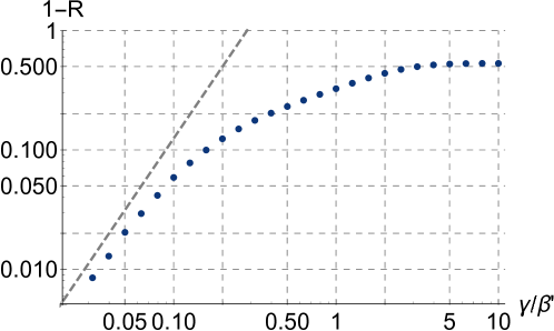
Figure 13: Plot for the deviation $1-R$ of the spectrum $\tilde{\Delta}$ from the one with $\gamma=0$, evaluated at $\tilde{k}=0.01$. The dashed line is proportional to $(\gamma/\beta^{\prime})^{2}$. It is shown that the data points behave $\propto(\gamma/\beta^{\prime})^{2}$ for small $\gamma/\beta^{\prime}$.

References

- [1] A. A. Starobinsky, “Spectrum of relict gravitational radiation and the early state of the universe,” JETP Lett. 30 (1979) 682–685. [Pisma Zh. Eksp. Teor. Fiz.30,719(1979)].
- [2] S. Y. Khlebnikov and I. I. Tkachev, “Relic gravitational waves produced after preheating,” Phys. Rev. D56 (1997) 653–660, arXiv:hep-ph/9701423 [hep-ph].
- [3] A. Vilenkin and E. P. S. Shellard, Cosmic Strings and Other Topological Defects. Cambridge University Press, 2000. http://www.cambridge.org/mw/academic/subjects/physics/theoretical-physics-and-mathematical-physics/cosmic-strings-and-other-topological-defects?format=PB.
- [4] E. Witten, “Cosmic Separation of Phases,” Phys. Rev. D30 (1984) 272–285.
- [5] C. J. Hogan, “Gravitational radiation from cosmological phase transitions,” Mon. Not. Roy. Astron. Soc. 218 (1986) 629–636.
- [6] LIGO Scientific Collaboration, J. Aasi et al., “Advanced LIGO,” Class. Quant. Grav. 32 (2015) 074001, arXiv:1411.4547 [gr-qc].
- [7] KAGRA Collaboration, K. Somiya, “Detector configuration of KAGRA: The Japanese cryogenic gravitational-wave detector,” Class. Quant. Grav. 29 (2012) 124007, arXiv:1111.7185 [gr-qc].
- [8] VIRGO Collaboration, F. Acernese et al., “Advanced Virgo: a second-generation interferometric gravitational wave detector,” Class. Quant. Grav. 32 no. 2, (2015) 024001, arXiv:1408.3978 [gr-qc].
- [9] Virgo, LIGO Scientific Collaboration, B. P. Abbott et al., “Observation of Gravitational Waves from a Binary Black Hole Merger,” Phys. Rev. Lett. 116 no. 6, (2016) 061102, arXiv:1602.03837 [gr-qc].
- [10] Virgo, LIGO Scientific Collaboration, B. P. Abbott et al., “GW151226: Observation of Gravitational Waves from a 22-Solar-Mass Binary Black Hole Coalescence,” Phys. Rev. Lett. 116 no. 24, (2016) 241103, arXiv:1606.04855 [gr-qc].
- [11] VIRGO, LIGO Scientific Collaboration, B. P. Abbott et al., “GW170104: Observation of a 50-Solar-Mass Binary Black Hole Coalescence at Redshift 0.2,” Phys. Rev. Lett. 118 no. 22, (2017) 221101, arXiv:1706.01812 [gr-qc].
- [12] eLISA Collaboration, P. A. Seoane et al., “The Gravitational Universe,” arXiv:1305.5720 [astro-ph.CO].
- [13] N. Seto, S. Kawamura, and T. Nakamura, “Possibility of direct measurement of the acceleration of the universe using 0.1-Hz band laser interferometer gravitational wave antenna in space,” Phys. Rev. Lett. 87 (2001) 221103, arXiv:astro-ph/0108011 [astro-ph].
- [14] G. M. Harry, P. Fritschel, D. A. Shaddock, W. Folkner, and E. S. Phinney, “Laser interferometry for the big bang observer,” Class. Quant. Grav. 23 (2006) 4887–4894. [Erratum: Class. Quant. Grav.23,7361(2006)].
- [15] K. Kajantie, M. Laine, K. Rummukainen, and M. E. Shaposhnikov, “Is there a hot electroweak phase transition at m(H) larger or equal to m(W)?,” Phys. Rev. Lett. 77 (1996) 2887–2890, arXiv:hep-ph/9605288 [hep-ph].
- [16] M. Gurtler, E.-M. Ilgenfritz, and A. Schiller, “Where the electroweak phase transition ends,” Phys. Rev. D56 (1997) 3888–3895, arXiv:hep-lat/9704013 [hep-lat].
- [17] F. Csikor, Z. Fodor, and J. Heitger, “Endpoint of the hot electroweak phase transition,” Phys. Rev. Lett. 82 (1999) 21–24, arXiv:hep-ph/9809291 [hep-ph].
- [18] R. Jinno and M. Takimoto, “Probing classically conformal model with gravitational waves,” Phys. Rev. D95 no. 1, (2017) 015020, arXiv:1604.05035 [hep-ph].
- [19] A. Kobakhidze, C. Lagger, A. Manning, and J. Yue, “Gravitational waves from a supercooled electroweak phase transition and their detection with pulsar timing arrays,” arXiv:1703.06552 [hep-ph].
- [20] S. Iso, P. D. Serpico, and K. Shimada, “QCD-Electroweak first order phase transition in supercooled universe,” arXiv:1704.04955 [hep-ph].
- [21] J. R. Espinosa, T. Konstandin, J. M. No, and M. Quiros, “Some Cosmological Implications of Hidden Sectors,” Phys. Rev. D78 (2008) 123528, arXiv:0809.3215 [hep-ph].
- [22] S. J. Huber, T. Konstandin, G. Nardini, and I. Rues, “Detectable Gravitational Waves from Very Strong Phase Transitions in the General NMSSM,” JCAP 1603 no. 03, (2016) 036, arXiv:1512.06357 [hep-ph].
- [23] L. Leitao and A. Megevand, “Gravitational waves from a very strong electroweak phase transition,” JCAP 1605 no. 05, (2016) 037, arXiv:1512.08962 [astro-ph.CO].
- [24] R.-G. Cai, M. Sasaki, and S.-J. Wang, “The gravitational waves from the first-order phase transition with a dimension-six operator,” JCAP 1708 no. 08, (2017) 004, arXiv:1707.03001 [astro-ph.CO].
- [25] A. Ashoorioon and T. Konstandin, “Strong electroweak phase transitions without collider traces,” JHEP 07 (2009) 086, arXiv:0904.0353 [hep-ph]. J. Kang, P. Langacker, T. Li, and T. Liu, “Electroweak Baryogenesis, CDM and Anomaly-free Supersymmetric U(1)’ Models,” JHEP 04 (2011) 097, arXiv:0911.2939 [hep-ph]. M. Jarvinen, C. Kouvaris, and F. Sannino, “Gravitational Techniwaves,” Phys. Rev. D81 (2010) 064027, arXiv:0911.4096 [hep-ph]. T. Konstandin, G. Nardini, and M. Quiros, “Gravitational Backreaction Effects on the Holographic Phase Transition,” Phys. Rev. D82 (2010) 083513, arXiv:1007.1468 [hep-ph]. V. Barger, D. J. H. Chung, A. J. Long, and L.-T. Wang, “Strongly First Order Phase Transitions Near an Enhanced Discrete Symmetry Point,” Phys. Lett. B710 (2012) 1–7, arXiv:1112.5460 [hep-ph]. L. Leitao, A. Megevand, and A. D. Sanchez, “Gravitational waves from the electroweak phase transition,” JCAP 1210 (2012) 024, arXiv:1205.3070 [astro-ph.CO]. G. C. Dorsch, S. J. Huber, and J. M. No, “Cosmological Signatures of a UV-Conformal Standard Model,” Phys. Rev. Lett. 113 (2014) 121801, arXiv:1403.5583 [hep-ph]. J. Kozaczuk, S. Profumo, L. S. Haskins, and C. L. Wainwright, “Cosmological Phase Transitions and their Properties in the NMSSM,” JHEP 01 (2015) 144, arXiv:1407.4134 [hep-ph]. P. Schwaller, “Gravitational Waves from a Dark Phase Transition,” Phys. Rev. Lett. 115 no. 18, (2015) 181101, arXiv:1504.07263 [hep-ph]. M. Kakizaki, S. Kanemura, and T. Matsui, “Gravitational waves as a probe of extended scalar sectors with the first order electroweak phase transition,” Phys. Rev. D92 no. 11, (2015) 115007, arXiv:1509.08394 [hep-ph]. R. Jinno, K. Nakayama, and M. Takimoto, “Gravitational waves from the first order phase transition of the Higgs field at high energy scales,” Phys. Rev. D93 no. 4, (2016) 045024, arXiv:1510.02697 [hep-ph]. F. P. Huang, Y. Wan, D.-G. Wang, Y.-F. Cai, and X. Zhang, “Hearing the echoes of electroweak baryogenesis with gravitational wave detectors,” Phys. Rev. D94 no. 4, (2016) 041702, arXiv:1601.01640 [hep-ph]. M. Garcia-Pepin and M. Quiros, “Strong electroweak phase transition from Supersymmetric Custodial Triplets,” JHEP 05 (2016) 177, arXiv:1602.01351 [hep-ph]. J. Jaeckel, V. V. Khoze, and M. Spannowsky, “Hearing the signals of dark sectors with gravitational wave detectors,” Phys. Rev. D94 no. 10, (2016) 103519, arXiv:1602.03901 [hep-ph]. P. S. B. Dev and A. Mazumdar, “Probing the Scale of New Physics by Advanced LIGO/VIRGO,” Phys. Rev. D93 no. 10, (2016) 104001, arXiv:1602.04203 [hep-ph]. K. Hashino, M. Kakizaki, S. Kanemura, and T. Matsui, “Synergy between measurements of gravitational waves and the triple-Higgs coupling in probing the first-order electroweak phase transition,” Phys. Rev. D94 no. 1, (2016) 015005, arXiv:1604.02069 [hep-ph]. G. Barenboim and W.-I. Park, “Gravitational waves from first order phase transitions as a probe of an early matter domination era and its inverse problem,” Phys. Lett. B759 (2016) 430–438, arXiv:1605.03781 [astro-ph.CO]. A. Kobakhidze, A. Manning, and J. Yue, “Gravitational Waves from the Phase Transition of a Non-linearly Realised Electroweak Gauge Symmetry,” arXiv:1607.00883 [hep-ph]. K. Hashino, M. Kakizaki, S. Kanemura, P. Ko, and T. Matsui, “Gravitational waves and Higgs boson couplings for exploring first order phase transition in the model with a singlet scalar field,” Phys. Lett. B766 (2017) 49–54, arXiv:1609.00297 [hep-ph]. M. Artymowski, M. Lewicki, and J. D. Wells, “Gravitational wave and collider implications of electroweak baryogenesis aided by non-standard cosmology,” JHEP 03 (2017) 066, arXiv:1609.07143 [hep-ph]. J. Kubo and M. Yamada, “Scale genesis and gravitational wave in a classically scale invariant extension of the standard model,” JCAP 1612 no. 12, (2016) 001, arXiv:1610.02241 [hep-ph]. C. Balazs, A. Fowlie, A. Mazumdar, and G. White, “Gravitational waves at aLIGO and vacuum stability with a scalar singlet extension of the Standard Model,” Phys. Rev. D95 no. 4, (2017) 043505, arXiv:1611.01617 [hep-ph]. V. Vaskonen, “Electroweak baryogenesis and gravitational waves from a real scalar singlet,” Phys. Rev. D95 no. 12, (2017) 123515, arXiv:1611.02073 [hep-ph]. G. C. Dorsch, S. J. Huber, T. Konstandin, and J. M. No, “A Second Higgs Doublet in the Early Universe: Baryogenesis and Gravitational Waves,” JCAP 1705 no. 05, (2017) 052, arXiv:1611.05874 [hep-ph]. F. P. Huang and X. Zhang, “Probing the hidden gauge symmetry breaking through the phase transition gravitational waves,” arXiv:1701.04338 [hep-ph]. I. Baldes, “Gravitational waves from the asymmetric-dark-matter generating phase transition,” JCAP 1705 no. 05, (2017) 028, arXiv:1702.02117 [hep-ph]. W. Chao, H.-K. Guo, and J. Shu, “Gravitational Wave Signals of Electroweak Phase Transition Triggered by Dark Matter,” arXiv:1702.02698 [hep-ph]. A. Beniwal, M. Lewicki, J. D. Wells, M. White, and A. G. Williams, “Gravitational wave, collider and dark matter signals from a scalar singlet electroweak baryogenesis,” arXiv:1702.06124 [hep-ph]. A. Addazi and A. Marciano, “Gravitational waves from dark first order phase transitions and dark photons,” arXiv:1703.03248 [hep-ph]. K. Tsumura, M. Yamada, and Y. Yamaguchi, “Gravitational wave from dark sector with dark pion,” arXiv:1704.00219 [hep-ph]. L. Marzola, A. Racioppi, and V. Vaskonen, “Phase transition and gravitational wave phenomenology of scalar conformal extensions of the Standard Model,” Eur. Phys. J. C77 no. 7, (2017) 484, arXiv:1704.01034 [hep-ph]. L. Bian, H.-K. Guo, and J. Shu, “Gravitational Waves, baryon asymmetry of the universe and electric dipole moment in the CP-violating NMSSM,” arXiv:1704.02488 [hep-ph]. F. P. Huang and J.-H. Yu, “Explore Inert Dark Matter Blind Spots with Gravitational Wave Signatures,” arXiv:1704.04201 [hep-ph]. A. Addazi and A. Marciano, “Limiting Majoron self-interactions from Gravitational waves experiments,” arXiv:1705.08346 [hep-ph]. Z. Kang, P. Ko, and T. Matsui, “Strong First Order EWPT and Strong Gravitational Waves in -symmetric Singlet Scalar Extension,” arXiv:1706.09721 [hep-ph]. W. Chao, W.-F. Cui, H.-K. Guo, and J. Shu, “Gravitational Wave Imprint of New Symmetry Breaking,” arXiv:1707.09759 [hep-ph].
- [26] C. Caprini et al., “Science with the space-based interferometer eLISA. II: Gravitational waves from cosmological phase transitions,” JCAP 1604 no. 04, (2016) 001, arXiv:1512.06239 [astro-ph.CO].
- [27] R.-G. Cai, Z. Cao, Z.-K. Guo, S.-J. Wang, and T. Yang, “The Gravitational-Wave Physics,” arXiv:1703.00187 [gr-qc].
- [28] A. Kosowsky, M. S. Turner, and R. Watkins, “Gravitational radiation from colliding vacuum bubbles,” Phys. Rev. D45 (1992) 4514–4535.
- [29] A. Kosowsky, M. S. Turner, and R. Watkins, “Gravitational waves from first order cosmological phase transitions,” Phys. Rev. Lett. 69 (1992) 2026–2029.
- [30] A. Kosowsky and M. S. Turner, “Gravitational radiation from colliding vacuum bubbles: envelope approximation to many bubble collisions,” Phys. Rev. D47 (1993) 4372–4391, arXiv:astro-ph/9211004 [astro-ph].
- [31] M. Kamionkowski, A. Kosowsky, and M. S. Turner, “Gravitational radiation from first order phase transitions,” Phys. Rev. D49 (1994) 2837–2851, arXiv:astro-ph/9310044 [astro-ph].
- [32] M. Hindmarsh, S. J. Huber, K. Rummukainen, and D. J. Weir, “Gravitational waves from the sound of a first order phase transition,” Phys. Rev. Lett. 112 (2014) 041301, arXiv:1304.2433 [hep-ph].
- [33] M. Hindmarsh, S. J. Huber, K. Rummukainen, and D. J. Weir, “Numerical simulations of acoustically generated gravitational waves at a first order phase transition,” Phys. Rev. D92 no. 12, (2015) 123009, arXiv:1504.03291 [astro-ph.CO].
- [34] M. Hindmarsh, S. J. Huber, K. Rummukainen, and D. J. Weir, “Shape of the acoustic gravitational wave power spectrum from a first order phase transition,” arXiv:1704.05871 [astro-ph.CO].
- [35] A. Kosowsky, A. Mack, and T. Kahniashvili, “Gravitational radiation from cosmological turbulence,” Phys. Rev. D66 (2002) 024030, arXiv:astro-ph/0111483 [astro-ph].
- [36] A. Nicolis, “Relic gravitational waves from colliding bubbles and cosmic turbulence,” Class. Quant. Grav. 21 (2004) L27, arXiv:gr-qc/0303084 [gr-qc].
- [37] C. Caprini and R. Durrer, “Gravitational waves from stochastic relativistic sources: Primordial turbulence and magnetic fields,” Phys. Rev. D74 (2006) 063521, arXiv:astro-ph/0603476 [astro-ph].
- [38] C. Caprini, R. Durrer, and G. Servant, “The stochastic gravitational wave background from turbulence and magnetic fields generated by a first-order phase transition,” JCAP 0912 (2009) 024, arXiv:0909.0622 [astro-ph.CO].
- [39] T. Kahniashvili, L. Kisslinger, and T. Stevens, “Gravitational Radiation Generated by Magnetic Fields in Cosmological Phase Transitions,” Phys. Rev. D81 (2010) 023004, arXiv:0905.0643 [astro-ph.CO].
- [40] A. Megevand and S. Ramirez, “Bubble nucleation and growth in very strong cosmological phase transitions,” Nucl. Phys. B919 (2017) 74–109, arXiv:1611.05853 [astro-ph.CO].
- [41] D. J. Weir, “Revisiting the envelope approximation: gravitational waves from bubble collisions,” Phys. Rev. D93 no. 12, (2016) 124037, arXiv:1604.08429 [astro-ph.CO].
- [42] C. Caprini, R. Durrer, and G. Servant, “Gravitational wave generation from bubble collisions in first-order phase transitions: An analytic approach,” Phys. Rev. D77 (2008) 124015, arXiv:0711.2593 [astro-ph].
- [43] R. Jinno and M. Takimoto, “Gravitational waves from bubble collisions: analytic derivation,” arXiv:1605.01403 [astro-ph.CO].
- [44] S. J. Huber and T. Konstandin, “Gravitational Wave Production by Collisions: More Bubbles,” JCAP 0809 (2008) 022, arXiv:0806.1828 [hep-ph].
- [45] R. Jinno and M. Takimoto, “Gravitational waves from bubble dynamics: Beyond the Envelope,” arXiv:1707.03111 [hep-ph].
- [46] J. R. Espinosa, T. Konstandin, J. M. No, and G. Servant, “Energy Budget of Cosmological First-order Phase Transitions,” JCAP 1006 (2010) 028, arXiv:1004.4187 [hep-ph].
- [47] T. Hahn, “CUBA: A Library for multidimensional numerical integration,” Comput. Phys. Commun. 168 (2005) 78–95, arXiv:hep-ph/0404043 [hep-ph].
- [48] M. Maggiore, Gravitational Waves. Vol. 1: Theory and Experiments. Oxford Master Series in Physics. Oxford University Press, 2007. http://www.oup.com/uk/catalogue/?ci=9780198570745.
- [49] B. Allen and J. D. Romano, “Detecting a stochastic background of gravitational radiation: Signal processing strategies and sensitivities,” Phys. Rev. D59 (1999) 102001, arXiv:gr-qc/9710117 [gr-qc].
- [50] E. Thrane and J. D. Romano, “Sensitivity curves for searches for gravitational-wave backgrounds,” Phys. Rev. D88 no. 12, (2013) 124032, arXiv:1310.5300 [astro-ph.IM].
- [51] A. D. Linde, “On the Vacuum Instability and the Higgs Meson Mass,” Phys. Lett. B70 (1977) 306–308.
- [52] A. D. Linde, “Decay of the False Vacuum at Finite Temperature,” Nucl. Phys. B216 (1983) 421. [Erratum: Nucl. Phys.B223,544(1983)].
- [53] L. Dolan and R. Jackiw, “Symmetry Behavior at Finite Temperature,” Phys. Rev. D9 (1974) 3320–3341.
- [54] P. B. Arnold and O. Espinosa, “The Effective potential and first order phase transitions: Beyond leading-order,” Phys. Rev. D47 (1993) 3546, arXiv:hep-ph/9212235 [hep-ph]. [Erratum: Phys. Rev.D50,6662(1994)].
- [55] S. Iso, N. Okada, and Y. Orikasa, “Classically conformal L extended Standard Model,” Phys. Lett. B676 (2009) 81–87, arXiv:0902.4050 [hep-ph].
- [56] S. Iso, N. Okada, and Y. Orikasa, “The minimal B-L model naturally realized at TeV scale,” Phys. Rev. D80 (2009) 115007, arXiv:0909.0128 [hep-ph].
- [57] C.-W. Chiang and E. Senaha, “On gauge dependence of gravitational waves from a first-order phase transition in classical scale-invariant models,” Phys. Lett. B774 (2017) 489–493, arXiv:1707.06765 [hep-ph].
- [58] W. A. Bardeen, “On naturalness in the standard model,” in Ontake Summer Institute on Particle Physics Ontake Mountain, Japan, August 27-September 2, 1995. 1995. http://lss.fnal.gov/cgi-bin/find_paper.pl?conf-95-391.
- [59] D. H. Lyth and E. D. Stewart, “Cosmology with a TeV mass GUT Higgs,” Phys. Rev. Lett. 75 (1995) 201–204, arXiv:hep-ph/9502417 [hep-ph].
- [60] D. H. Lyth and E. D. Stewart, “Thermal inflation and the moduli problem,” Phys. Rev. D53 (1996) 1784–1798, arXiv:hep-ph/9510204 [hep-ph].
- [61] R. Easther, J. T. Giblin, Jr., E. A. Lim, W.-I. Park, and E. D. Stewart, “Thermal Inflation and the Gravitational Wave Background,” JCAP 0805 (2008) 013, arXiv:0801.4197 [astro-ph].