Submitted to IEEE Transactions on Signal Processing
L1-norm Principal-Component Analysis of
Complex Data

Abstract

L1-norm Principal-Component Analysis (L1-PCA) of real-valued data has attracted significant research interest over the past decade. However, L1-PCA of complex-valued data remains to date unexplored despite the many possible applications (e.g., in communication systems). In this work, we establish theoretical and algorithmic foundations of L1-PCA of complex-valued data matrices. Specifically, we first show that, in contrast to the real-valued case for which an optimal polynomial-cost algorithm was recently reported by Markopoulos et al., complex L1-PCA is formally NP-hard in the number of data points. Then, casting complex L1-PCA as a unimodular optimization problem, we present the first two suboptimal algorithms in the literature for its solution. Our experimental studies illustrate the sturdy resistance of complex L1-PCA against faulty measurements/outliers in the processed data.

Index Terms — Data analytics, dimensionality reduction, erroneous data, faulty measurements, L1-norm, machine learning, principal-component analysis, outlier resistance.

I Introduction

For more than a century, Principal-Component Analysis (PCA) has been a core operation in data/signal processing [2, 3]. Conceptually, PCA can be viewed as the pursuit of a coordinate system (defined by the principal components) that reveals underlying linear trends of a data matrix. In its conventional form, the new coordinate system is calculated such that it preserves the energy content of the data matrix to the maximum possible extend. Conventionally, the energy content of a data point is expressed by means of its L2-norm –i.e., its Euclidean distance from the center of the coordinate system. Thus, for any complex data matrix $\mathbf{X}=[\mathbf{x}_{1},\mathbf{x}_{2},\ldots,\mathbf{x}_{N}]\in\mathbb{C}^{D\times N}$, PCA searches for the size-$K$ ($1\leq K<\text{rank}(\mathbf{X})$) orthonormal basis (or, $K$-dimensional coordinate system) that solves

$$\mathbf{Q}^{\text{opt}}_{L2}=\underset{\mathbf{Q}\in\mathbb{C}^{D\times K};~{}\mathbf{Q}^{H}\mathbf{Q}=\mathbf{I}_{K}}{\mathrm{argmax}}~{}{\|\mathbf{Q}^{H}\mathbf{X}\|_{2}}$$ (1)

where, for any $\mathbf{A}\in\mathbb{C}^{m\times n}$, its L2-norm is defined as $\|\mathbf{A}\|_{2}=\sqrt{\sum_{i=1}^{m}\sum_{j=1}^{n}|A_{i,j}|^{2}}$, $|\cdot|$ denotes the magnitude of a complex number (coinciding with the absolute value of a real number), and $\mathbf{I}_{K}$ is the size-$K$ identity matrix. Due to its definition in (1), PCA is also commonly referred to as L2-norm PCA, or simply L2-PCA.

A practical reason of the tremendous popularity of L2-PCA is the computational simplicity by which the solution to (1) can be obtained. Specifically, a solution matrix $\mathbf{Q}^{\text{opt}}_{L2}$ can be formed by the $K$ dominant singular vectors of $\mathbf{X}$ and is, thus, obtainable by means of Singular-Value Decomposition (SVD) of $\mathbf{X}$, with quadratic complexity in the number of data samples $N$ [5]. Moreover, L2-PCA is a scalable operation in the sense that the $(k+1)$-th PC can be calculated using directly the first $k$ PCs that are always preserved. In addition, there are several algorithms that can efficiently update the solution to (1) as new data points become available [6]. Finally, by the Projection Theorem [5] it is easy to show that the maximum-L2-norm-projection problem in (1) is equivalent to the familiar minimum-L2-norm-error problem

$$\underset{\begin{subarray}{c}\mathbf{Q}\in\mathbb{C}^{D\times K};~{}\mathbf{Q}^{H}\mathbf{Q}=\mathbf{I}_{K}\\ \mathbf{Z}\in\mathbb{C}^{K\times N}\end{subarray}}{\min.}{\|\mathbf{X}-\mathbf{Q}\mathbf{Z}\|_{2}}.$$ (2)

On the downside, conventional L2-PCA, seeking to maximize the L2-norm of the projected data-points in (1), is well-known to be overly sensitive to outlying measurements in the processed matrix. Such outliers may leek into the data matrix due to a number of different causes, such as sensing/hardware malfunctions, external interference, and errors in data storage or transcription. Regardless of their cause, outliers are described as unexpected, erroneous values that lie far from the nominal data subspace and affect tremendously a number of data analysis methods, including L2-PCA. Since the original conception of L2-PCA [2], engineers and mathematicians have been trying robustify its against outliers. Popular robust versions of PCA are weighted PCA (WPCA) [7, 8], influence-function PCA [9], and L1-norm PCA (or, simply L1-PCA) [11, 10, 12, 13, 14, 15, 16, 17, 18, 19, 20, 21, 22, 23, 24, 25, 26, 27, 28, 38, 1, 37, 36, 35, 34, 29, 30, 31, 32, 33].

From an algebraic viewpoint, of all robust versions of PCA, L1-PCA is arguably the most straightforward modification. Mathematically, L1-PCA of real-valued data is formulated as

$$\underset{\mathbf{Q}\in\mathbb{R}^{D\times K};~{}\mathbf{Q}^{T}\mathbf{Q}=\mathbf{I}_{K}}{\max.}{\|\mathbf{Q}^{T}\mathbf{X}\|_{1}}$$ (3)

where $\|\cdot\|_{1}$ is the L1-norm operator, such that for any $\mathbf{A}\in\mathbb{C}^{m\times n}$, $\|\mathbf{A}\|_{1}=\sum_{i=1}^{m}\sum_{j=1}^{n}|A_{i,j}|$. That is, L1-PCA derives from L2-PCA, by substituting the L2-norm with the more robust L1-norm. By not placing squared emphasis on the magnitude of each point (as L2-PCA does), L1-PCA is far more resistant to outlying, peripheral points. Importantly, thorough recent studies have shown that when the processed data are not outlier corrupted, then the solutions of L1-PCA and L2-PCA describe an almost identical subspace.

Due to its outlier resistance, L1-PCA of real-valued data matrices has attracted increased documented research interest in the past decade. Interestingly, it was shown that real-valued L1-PCA can be converted into a combinatorial problem over antipodal binary variables ($\pm 1$), solvable with intrinsic complexity polynomial in the data record size, $\mathcal{O}(N^{\text{rank}(\mathbf{X})K-K+1})$ [10].

Despite its increasing popularity for outlier-resistant processing real-valued data, L1-PCA for complex-data processing remains to date unexplored. Similar to (3), complex L1-PCA is formulated as

$$\mathbf{Q}^{\text{opt}}_{L1}=\underset{\mathbf{Q}\in\mathbb{C}^{D\times K};~{}\mathbf{Q}^{H}\mathbf{Q}=\mathbf{I}_{K}}{\mathrm{argmax}}~{}{\|\mathbf{Q}^{H}\mathbf{X}\|_{1}}.$$ (4)

Interestingly, in contrast to real-valued L1-PCA, complex L1-PCA in (4) has no obvious connection to a combinatorial problem. Moreover, no finite-step algorithm (exponential or otherwise) has ever been reported for optimally solving (4). Yet, as a robust analogous to complex L2-PCA, complex L1-PCA in (4) can be traced to many important applications that involve complex-valued measurements, e.g., in the fields communications, radar processing, or general signal processing, tailored to complex-domain transformations (such as Fourier) of real-valued data.

Our contributions in this present paper are summarized as follows.

1. We prove that (4) can be cast as an optimization problem over the set of unimodular matrices.

2. We provide the first two fast algorithms to solve (4) suboptimally.

3. We offer numerical studies that evaluate the performance of our complex L1-PCA algorithms.

Importantly, our numerical studies illustrate that the proposed complex L1-PCA exhibits sturdy resistance against outliers, while it performs similarly to L2-PCA when the processed data are outlier-free.

The rest of the paper is organized as follows. Section II offers as brief overview of technical preliminaries and notation. Section III is devoted to the presentation of out theoretical findings and the derivation of the proposed algorithms. Section IV holds our numerical studies. Finally, some concluding remarks are drawn in Section V.

II Preliminaries and Notation

Our subsequent algebraic developments involve extensively the sign of a complex number and the nuclear norm of a matrix. In this section, we provide the reader with the definitions of these two measures, as well as useful pertinent properties.

II.A The Sign of a Complex Number

Every complex number $z$ can be written as the product of its magnitude and a complex exponential. The complex exponential part is what we call “sign” of the complex number and is denoted by $\mathrm{sgn}\left(z\right)$. That is, $\forall z\in\mathbb{C}:~{}z=|z|\mathrm{sgn}\left(z\right)$, where $\mathrm{sgn}\left(z\right)\triangleq e^{j\angle z}$. Clearly, the sign of any complex number belongs to the unitary complex circle

$$U\triangleq\{z\in\mathbb{C}:~{}|z|=1\}.$$ (5)

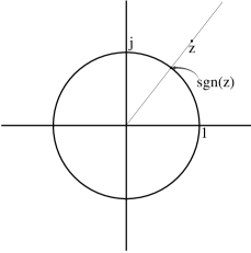
Figure 1: Graphical illustration of the sign of a complex number.

Fig. 1 shows that the sign of any non-zero complex number is unique and satisfies the property presented Lemma 1.

Lemma 1.

For every $z\in C$, with $|z|>0$, $\mathrm{sgn}\left(z\right)$ is the point on $U$ that lies nearest to $z$ in the magnitude sense. That is, $\mathrm{sgn}\left(z\right)=\underset{a\in U}{\mathrm{argmin}}~{}{|a-z|}$.

Through elementary algebraic manipulations, Lemma 1 implies that

$$\mathrm{sgn}\left(a\right)=\underset{b\in U}{\mathrm{argmax}}~{}{\Re\{b^{*}a\}}.$$ (6)

In addition, the optimal value of (6) is the magnitude of $a$. The above definition and properties of the sign can be generalized into vectors and matrices. Let us define the sign of a matrix $\mathbf{A}\in\mathbb{C}^{m\times n}$, for any $n$ and $m$, as the matrix that contains the signs of the individual entries of $\mathbf{A}$. That is, we define

$$\mathrm{sgn}\left(\mathbf{A}\right)\triangleq\left[\begin{array}[]{ccc}\mathrm{sgn}\left(a_{1,1}\right)&\dots&\mathrm{sgn}\left(a_{1,n}\right)\\ \vdots&\ddots&\vdots\\ \mathrm{sgn}\left(a_{m,1}\right)&\dots&\mathrm{sgn}\left(a_{m,n}\right)\end{array}\right].$$ (10)

In accordance to (6), the sign of $\mathbf{A}$ can be expressed as the solution to the maximization problem

$$\mathrm{sgn}\left(\mathbf{A}\right)=\underset{\mathbf{B}\in U^{n\times m}}{\mathrm{argmax}}~{}{\Re\{\mathrm{Tr}\left\{\mathbf{B}\mathbf{A}\right\}\}}.$$ (11)

Moreover, the optimal objective value of (11) is the L1-norm of $\mathbf{A}$; that is,

$$\|\mathbf{A}\|_{1}=\underset{\mathbf{B}\in U^{n\times m}}{\max}~{}{\Re\{\mathrm{Tr}\left\{\mathbf{B}\mathbf{A}\right\}\}}=\mathrm{Tr}\left\{\text{sgn}(\mathbf{A})^{H}\mathbf{A}\right\}.$$ (12)

Finally, by the above definitions it holds that the sign of the product of two complex numbers equals the product of individual signs. In addition, it is clear that the sign of a number is $+1$ if-and-only-if the number is real and positive and $-1$ if-and-only-if the number is real and negative.

II.B The Nuclear Norm

Consider matrix $\mathbf{A}\in\mathbb{C}^{m\times n}$, with $m>n$ with no loss of generality. Then, let $\mathbf{A}$ admit SVD $\mathbf{A}\overset{svd}{=}\mathbf{U}\text{Diag}(\boldsymbol{\sigma})\mathbf{V}^{H}$, where $\mathbf{U}^{H}\mathbf{U}=\mathbf{V}^{H}\mathbf{V}=\mathbf{I}_{n}$ and $\boldsymbol{\sigma}\in\mathbb{R}_{\geq 0}^{n}$ contains the singular values of $\mathbf{A}$ in descending order (i.e., $\sigma_{1}\geq\sigma_{2}\geq\ldots\geq\sigma_{n}$). The nuclear norm of $\mathbf{A}$ is then defined as the summation of the singular values of $\mathbf{A}$,

$$\|\mathbf{A}\|_{*}\triangleq\sum_{i=1}^{r}\sigma_{i}=\|\boldsymbol{\sigma}\|_{1}.$$ (13)

Clearly, it holds that $\|\mathbf{A}\|_{*}=\|\mathbf{A}^{H}\|_{*}$. Being a fundamental quantity in linear algebra, the nuclear norm can be expressed in several different ways. For example, in connection to the Orthogonal Procrustes Theorem [39, 5], it holds that

$$\|A\|_{*}=\underset{\mathbf{Q}\in\mathbb{C}^{m\times n};~{}\mathbf{Q}^{H}\mathbf{Q}=\mathbf{I}_{n}}{\max}~{}{\Re\{\mathrm{Tr}\left\{\mathbf{Q}^{H}\mathbf{A}\right\}\}}.$$ (14)

Moreover, denoting by $\text{unt}(\mathbf{A})$ the $m\times n$ unitary matrix that maximizes (14) and assuming that $\mathbf{A}$ has full column rank (i.e., $\text{rank}(\mathbf{A})=n$), it holds that

$$\mathbf{A}=\text{unt}(\mathbf{A})(\mathbf{A}^{H}\mathbf{A})^{\frac{1}{2}},$$ (15)

which is known as the polar decomposition of $\mathbf{A}$ [40, 5]. Finally, $\text{unt}(\mathbf{A})$ can calculated by the SVD of $\mathbf{A}$ as

$$\mathrm{unt}\left(\mathbf{A}\right)=\mathbf{U}\mathbf{V}^{H}.$$ (16)

Based on the above preliminaries, in the following section we present our developments on complex L1-PCA.

III Complex L1-PCA

III.A Problem Connection to Unimodular Optimization

In view of (11) and (14) we can rewrite the complex L1-PCA problem in (4) as

$$\underset{\mathbf{Q}\in\mathbb{C}^{D\times K};~{}\mathbf{Q}^{H}\mathbf{Q}=\mathbf{I}_{K}}{\max}~{}{\|\mathbf{Q}^{H}\mathbf{X}\|_{1}} =\underset{{\mathbf{Q}\in\mathbb{C}^{D\times K};~{}\mathbf{Q}^{H}\mathbf{Q}=I_{K}}}{\max}~{}{\mathrm{Tr}\left\{\text{sgn}(\mathbf{Q}^{H}\mathbf{X})^{H}\mathbf{Q}^{H}\mathbf{X}\right\}}$$ (17)

$$\overset{\eqref{sgn_prop1_mat}}{=}\underset{\begin{subarray}{c}\mathbf{Q}\in\mathbb{C}^{D\times K};~{}\mathbf{Q}^{H}\mathbf{Q}=I_{K}\\ \mathbf{B}\in U^{N\times K}\end{subarray}}{\max}~{}{\Re\left\{\mathrm{Tr}\left\{\mathbf{B}\mathbf{Q}^{H}\mathbf{X}\right\}\right\}}$$ (18)

$$\overset{\eqref{proc_label}}{=}\underset{\mathbf{B}\in U^{N\times K}}{\max}~{}{\|\mathbf{X}\mathbf{B}\|_{*}}.$$ (19)

That is, complex L1-PCA is directly connected to a maximization problem over the set of $N\times K$ unimodular matrices. Interestingly, Markopoulos et. al. [10, 12] have proven a similar result for the real case. Specifically, [10] reformulated real-valued L1-PCA to a nuclear-norm maximization over the set of $N\times K$ $(\pm 1)$-valued matrices, $\{\pm 1\}^{N\times K}$. Considering that $\{\pm 1\}$ is in fact the intersection of $U$ with the axis of real numbers, we realize that the binary-nuclear-norm maximization to which real-valued L1-PCA corresponds [10] constitutes a relaxation of the unimodular-nuclear-norm maximization in (19). Due to the finite size of $\{\pm 1\}^{N\times K}$, finite-step algorithms could be devised for the solution of real-valued L1-PCA. Regretfully, since $U^{N\times K}$ has uncountably infinite elements, this is not the case for complex L1-PCA.

Even though unimodular-nuclear-norm maximization in (19) cannot be solved exhaustively, there are still necessary optimality conditions that we can use to devise efficient algorithms for solving it at least locally. The following proposition introduces the first of these optimality conditions.

Proposition 1.

Let $(\mathbf{Q}_{L}1^{\text{opt}},\mathbf{B}^{\text{opt}})$ be an optimal solution pair for (18). Then, it holds that

$$\mathbf{Q}_{L1}^{\text{opt}}=\mathrm{unt}\left(\mathbf{X}\mathbf{B}^{\text{opt}}\right)~{}~{}\text{and}~{}~{}\mathbf{B}^{\text{opt}}=\mathrm{sgn}\left(\mathbf{X}^{H}\mathbf{Q}_{L1}^{\text{opt}}\right).$$ (20)

Moreover, $\mathbf{Q}_{L1}^{\text{opt}}$ is a solution to (4) and $\mathbf{B}^{\text{opt}}$ is a solution to (19).

Proposition 1 derives directly from (11), (14), and the fact that both (4) and (19) are equivalent to (18). Most importantly, this proposition establishes that, if $\mathbf{B}^{\text{opt}}$ is a solution to (19), then $\mathbf{Q}^{\text{opt}}_{L1}=\mathrm{unt}\left(\mathbf{X}\mathbf{B}^{\text{opt}}\right)$ is a solution to the L1-PCA in (4). Thus, one can focus on solving (19) and then use its solution to derive the L1-PCs by means of simple SVD (see the definition of $\mathrm{unt}\left(\cdot\right)$ in (16)). In addition, the two equations in (20) can be combined into forming a new pair of necessary optimality conditions that concern the individual problems (4) and (19). The new optimality conditions are presented in the following Corollary 1.

Corollary 1.

Let $\mathbf{Q}_{L1}^{\text{opt}}$ be a solution to (4); then, it holds that $\mathbf{Q}_{L1}^{\text{opt}}=\mathrm{unt}\left(\mathbf{X}\mathrm{sgn}\left(\mathbf{X}^{H}\mathbf{Q}_{L1}^{\text{opt}}\right)\right)$. Let $\mathbf{B}^{\text{opt}}$ be a solution to (19); then, it holds that $\mathbf{B}^{\text{opt}}=\mathrm{sgn}\left(\mathbf{X}^{H}\mathrm{unt}\left(\mathbf{X}\mathbf{B}^{\text{opt}}\right)\right)$.

III.B Complex L1-PCA when rank$(\mathbf{X})<D$

Consider $\mathbf{X}\in\mathbb{C}^{D\times N}$ with $r=\text{rank}(\mathbf{X})<D$. $\mathbf{X}$ admits thin SVD $\mathbf{X}\overset{svd}{=}\mathbf{U}_{x}\mathbf{S}_{x}\mathbf{V}_{x}^{H}$, where $\mathbf{U}_{x}^{H}\mathbf{U}_{x}=\mathbf{V}_{x}^{H}\mathbf{V}_{x}=\mathbf{I}_{r}$ and $\mathbf{S}_{x}$ is the $r\times r$ diagonal matrix that contains the non-zero singular values of $\mathbf{X}$. In accordance to (3) above, to obtain the $K\leq r$ L1-PCs of $\mathbf{X}$, $\mathbf{Q}^{\text{opt}}_{L1}$, we can work in two steps: (i) obtain the solution $\mathbf{B}^{\text{opt}}$ to (19) and (ii) conduct SVD on $\mathbf{X}\mathbf{B}^{\text{opt}}$ and return $\mathbf{Q}^{\text{opt}}_{L1}=\mathrm{unt}\left(\mathbf{X}\mathbf{B}^{\text{opt}}\right)$. Let us focus for a moment on the first step. We observe that

$$\|\mathbf{X}\mathbf{B}\|_{*} =\|\mathbf{U}_{x}\mathbf{S}_{x}\mathbf{V}_{x}^{H}\mathbf{B}\|_{*}$$ (21)

$$=\text{Tr}(\sqrt{(\mathbf{U}_{x}\mathbf{S}_{x}\mathbf{V}_{x}^{H}\mathbf{B})^{H}\mathbf{U}_{x}\mathbf{S}_{x}\mathbf{V}_{x}^{H}\mathbf{B}})$$ (22)

$$=\text{Tr}(\sqrt{\mathbf{B}^{H}\mathbf{V}_{x}^{H}\mathbf{S}_{x}^{H}\mathbf{S}_{x}\mathbf{V}_{x}^{H}\mathbf{B}})$$ (23)

$$=\|\mathbf{S}_{x}\mathbf{V}_{x}^{H}\mathbf{B}\|_{*}=\|\mathbf{X}_{short}\mathbf{B}\|_{*}$$ (24)

where $\mathbf{X}_{short}\triangleq\mathbf{S}_{x}\mathbf{V}_{x}^{H}\in\mathbb{C}^{r\times N}$. Then, $\mathbf{B}^{\text{opt}}$ maximizes both (21) (by definition) and (24) (by equivalence). Notice also that $\mathrm{unt}\left(\mathbf{X}\mathbf{B}^{\text{opt}}\right)=\mathbf{U}_{x}\mathrm{unt}\left(\mathbf{X}_{short}\mathbf{B}^{\text{opt}}\right)$. By the above analysis, the following proposition holds true.

Proposition 2.

Consider $\mathbf{X}\in\mathbb{C}^{D\times N}$, with $r=\text{rank}(\mathbf{X})\leq\min\{D,N\}$, admitting thin SVD $\mathbf{X}=\mathbf{U}_{x}\mathbf{S}_{x}\mathbf{V}_{x}^{H}$ (i.e., $\mathbf{S}_{x}$ is $r\times r$). Define $\mathbf{X}_{short}=\mathbf{S}_{X}\mathbf{V}_{x}^{H}$. Let the $\mathbf{Q}^{\text{opt}}_{L1,short}\in\mathbb{C}^{r\times K}$ be the $K<r$ L1-PCs of $\mathbf{X}_{short}$, solution to $\underset{\mathbf{Q}\in\mathbb{C}^{r\times K};~{}\mathbf{Q}^{H}\mathbf{Q}=\mathbf{I}_{K}}{max.}~{}\|\mathbf{Q}^{H}\mathbf{X}_{short}\|_{1}$. Then, it holds that

$$\mathbf{Q}^{\text{opt}}_{L1}=\mathbf{U}_{x}\mathbf{Q}^{\text{opt}}_{L1,short}$$ (25)

is the solution to the L1-PCA in (4). Moreover, $\|{\mathbf{Q}^{\text{opt}}_{L1}}^{H}\mathbf{X}\|_{1}=\|\mathbf{X}\mathbf{B}^{\text{opt}}\|_{*}=\|\mathbf{X}_{short}\mathbf{B}^{\text{opt}}\|_{*}=\|{\mathbf{Q}^{\text{opt}}_{L1,short}}^{H}\mathbf{X}_{short}\|_{1}$.

Proposition 2 shows that the L1-PCs of a rank-$r$ $D\times N$ matrix can always be obtained through the L1-PCA of a rank-$r$ $r\times N$ matrix. Therefore, Proposition 2 steers our algorithmic focus to problems where $\mathbf{X}$ has full row-rank (i.e., $D=r=\text{rank}(\mathbf{X})$).

III.C The Single-Component Case and L1-PCA Hardness

In its simplest non-trivial form, complex L1-PCA is the search of a single ($K=1$) component $\mathbf{q}\in\mathbb{C}^{D\times 1}$ such that $\|\mathbf{q}^{H}X\|_{1}$ is maximized. In accordance to our more generic developments for the multi-component ($K\geq 1$) case above, the pursuit of a single L1-PC can also be rewritten as a unimodular nuclear-norm maximization. That is,

$$\underset{\mathbf{q}\in C^{D};\|\mathbf{q}\|_{2}=1}{\max}~{}\|\mathbf{q}^{H}\mathbf{X}\|_{1} =\underset{\mathbf{b}\in U^{N\times 1}}{\max}~{}\|\mathbf{X}\mathbf{b}\|_{*}$$ (26)

$$=\underset{\mathbf{b}\in U^{N\times 1}}{\max}~{}\|\mathbf{X}\mathbf{b}\|_{2}=\sqrt{\underset{\mathbf{b}\in U^{N\times 1}}{\max}~{}\mathbf{b}^{H}\mathbf{X}^{H}\mathbf{X}\mathbf{b}}.$$ (27)

Equation in (27) derives by the fact that any complex vector $\mathbf{a}\in\mathbb{C}^{m}$ admits SVD $\mathbf{a}\overset{svd}{=}\mathbf{u}\sigma$, with $\mathbf{u}=\mathbf{a}\|\mathbf{a}\|_{2}^{-1}$ and $\sigma=\|\mathbf{a}\|_{2}$ (trivially, the dominant right-hand singular vector is $1$). By Proposition 1, for the L1-PC $\mathbf{q}^{\text{opt}}_{L1}$ that solves (26) it holds

$$\mathbf{q}^{\text{opt}}_{L1}=\mathrm{unt}\left(\mathbf{X}\mathbf{b}^{\text{opt}}\right)=\mathbf{X}\mathbf{b}^{\text{opt}}\|\mathbf{X}\mathbf{b}^{\text{opt}}\|_{2}^{-1},$$ (28)

where $\mathbf{b}^{\text{opt}}$ is the solution to (27). Also, $\mathbf{b}^{\text{opt}}=\mathrm{sgn}\left(\mathbf{X}^{H}\mathbf{q}^{\text{opt}}_{L1}\right)$.

The unimodular quadratic maximization (UQM) problem in (27) is a well-studied problem in the literature, with several interesting applications, including among others the design of maximum-signal-to-interference-plus-noise-ratio (max-SINR) phased-arrays and and the design of unomodular codes [41]. For the real-data case, UQM in (27) takes the form of the well- binary-quadratic-maximization [42], as proven in [10].

Certainly, the necessary optimality condition presented in Corollary 1 for (19) also applies to (27). Specifically, if $\mathbf{b}^{\text{opt}}$ is a solution to (27), then

$$\mathbf{b}^{\text{opt}}=\mathrm{sgn}\left(\mathbf{X}^{H}\mathrm{unt}\left(\mathbf{X}\mathbf{b}^{\text{opt}}\right)\right)=\mathrm{sgn}\left(\mathbf{X}^{H}\mathbf{X}\mathbf{b}^{\text{opt}}\right).$$ (29)

However, in contrast to what has been conjectured for the real case [19, 20] for the real case, (29) is not a sufficient condition for local optimality. The reason is that $\mathbf{b}=\mathrm{sgn}\left(\mathbf{X}^{H}\mathbf{X}\mathbf{b}\right)$ is also satisfied by some “saddle” points of $\|\mathbf{X}\mathbf{b}\|_{2}$. In this section we provide a stronger optimality condition than (29), that is necessary and sufficient for local optimality.

For compactness in notation, we begin by defining

$$\boldsymbol{\omega}(\mathbf{b})\triangleq\mathbf{b}^{*}\odot(\mathbf{X}^{H}\mathbf{X}\mathbf{b})\in\mathbb{C}^{N\times 1},$$ (30)

for any $\mathbf{b}\in U^{N}$, where $(\cdot)^{*}$ performs complex-conjugation and $\odot$ is the element-wise product (Hadamard) operator. Even though the entries of $\boldsymbol{\omega}(\mathbf{b})$ are complex, their summation $\sum_{n=1}^{N}\omega_{n}$ is real and positive, equal to the quadratic form $\mathbf{b}^{H}\mathbf{X}^{H}\mathbf{X}\mathbf{b}$. The following Proposition 3 presents a necessary condition for optimality in the UQM of (27) that is satisfied by all local maximizers, but not by minimizers or saddle points.

Proposition 3.

A unimodular vector ${\mathbf{b}}$ is a local maximizer to (27), if-and-only-if

$${\omega}_{n}(\mathbf{b})\in\mathbb{R}\text{~{}~{}and~{}~{}}{\omega}_{n}(\mathbf{b})\geq\|\mathbf{x}_{n}\|_{2}^{2}~{}~{}~{}\forall n\in\{1,\ldots,N\}.$$ (31)

Proof. For any $\mathbf{b}\in U^{N\times 1}$ there is an angle-vector $\boldsymbol{\phi}\in[0,2\pi)^{N\times 1}$ such that $\mathbf{b}=e^{j\boldsymbol{\phi}}=[e^{j\phi_{1}},\dots,e^{j\phi_{N}}]^{T}$. The quadratic in the UQM of (27) can be then rewritten as $(e^{j\boldsymbol{\phi}})^{H}\mathbf{X}^{H}\mathbf{X}(e^{j\boldsymbol{\phi}})$, which is a function continuously twice differentiable in the angle-vector $\boldsymbol{\phi}$; the corresponding first and second derivatives are

$$\mathbf{g}(\mathbf{b}) =2\Im\{\boldsymbol{\omega}(\mathbf{b})\}\text{~{}~{}and}$$ (32)

$$\mathbf{H}(\mathbf{b}) =2\Re\Big{\{}\mathrm{Diag}(\mathbf{b})^{H}\mathbf{X}^{H}\mathbf{X}\mathrm{Diag}(\mathbf{b})-\mathrm{Diag}(\boldsymbol{\omega}(\mathbf{b}))\Big{\}},$$ (33)

respectively. Any local maximizer of (27) will null the gradient and render the Hessian in (33) negative-semidefinite. In the sequel we prove both directions of the equivalence (“if-and-only-if” statement) in Proposition 3.

Direct

If ${\mathbf{b}}$ is local maximizer of (27) then $\mathbf{H}(\mathbf{b})\preceq 0$. Therefore, for every $n\in\{1,2,\ldots,N\}$,

$$\mathbf{e}_{n}^{T}\mathbf{H}(\mathbf{b})\mathbf{e}_{n}\leq 0~{}\Leftrightarrow~{}2\Re\Big{\{}b_{n}^{*}\mathbf{x}_{n}^{H}\mathbf{x}_{n}b_{n}-\omega_{n}(\mathbf{b})\Big{\}}\leq 0~{}\Leftrightarrow~{}\omega_{n}(\mathbf{b})\geq\|\mathbf{x}_{n}\|_{2}^{2},$$ (34)

where $\mathbf{e}_{n}$ the $n$-th column of $\mathbf{I}_{N}$.

Reverse

Consider ${\mathbf{b}}$ such that all entries of ${\boldsymbol{\omega}}(\mathbf{b})$ satisfy (31). Then, for every $\mathbf{z}\in\mathbb{C}^{N}$,

$$\mathbf{z}^{T}\mathbf{H}(\mathbf{b})\mathbf{z} =2\mathbf{z}^{T}\left(\mathrm{Diag}({\mathbf{b}})^{H}\mathbf{X}^{H}\mathbf{X}\mathrm{Diag}({\mathbf{b}})-\mathrm{Diag}({\boldsymbol{\omega}}(\mathbf{b}))\right)\mathbf{z}$$ (35)

$$=2\left\|\sum_{n=1}^{N}z_{n}b_{n}\mathbf{x}_{n}\right\|_{2}^{2}-2\sum_{n=1}^{N}z_{n}^{2}\omega_{n}(\mathbf{b})$$ (36)

$$\leq 2\sum_{n=1}^{N}\left\|z_{n}b_{n}\mathbf{x}_{n}\right\|_{2}^{2}-2\sum_{n=1}^{N}z_{n}^{2}\omega_{n}(\mathbf{b})$$ (37)

$$=2\sum_{n=1}^{N}z_{n}^{2}\left(\left\|\mathbf{x}_{n}\right\|_{2}^{2}-\omega_{n}(\mathbf{b})\right)\leq 0$$ (38)

which implies that the Hessian at $\mathbf{b}$, $\mathbf{H}(\mathbf{b})$, is negative-semidefinite. This, in turn, implies that $\hat{\mathbf{b}}$ is a local maximizer of (27). $\square$

In the sequel, we present a direct Corollary of Proposition 3.

Corollary 2.

A unimodular vector ${\mathbf{b}}$ is a local maximizer to (27), if-and-only-if

$${\mathbf{b}}=\mathrm{sgn}\left(\mathbf{A}_{d}{\mathbf{b}}\right)$$ (39)

where $\mathbf{A}_{d}\triangleq\mathbf{X}^{H}\mathbf{X}-\text{Diag}([\|\mathbf{x}_{1}\|_{2}^{2},\ldots,\|\mathbf{x}_{N}\|_{2}^{2}]^{T})$.

Proof. In view of the sign of the previous section, for every $n\in\{1,2,\ldots,N\}$ it holds

$$\omega_{n}(\mathbf{b})\geq\|\mathbf{x}_{n}\|_{2}^{2} \Leftrightarrow\omega_{n}(\mathbf{b})-\|\mathbf{x}_{n}\|_{2}^{2}\geq 0$$ (40)

$$\Leftrightarrow\mathrm{sgn}\left(\omega_{n}(\mathbf{b})-\|\mathbf{x}_{n}\|_{2}^{2}\right)=1$$ (41)

$$\Leftrightarrow\mathrm{sgn}\left(b_{n}^{*}\mathbf{x}^{H}\mathbf{X}{\mathbf{b}}-\|\mathbf{x}_{n}\|_{2}^{2}\right)=1$$ (42)

$$\Leftrightarrow b_{n}=\mathrm{sgn}\left(\sum_{m\neq n}\mathbf{x}_{n}^{H}\mathbf{x}_{m}b_{m}\right)$$ (43)

which, by the definition of $\mathbf{A}_{d}$, implies (39). $\square$

The quantitative difference between the conditions (29) and (39) lie in the corresponding $\boldsymbol{\omega}(\cdot)$ variables. On the one hand, condition in (29) guarantees that $\omega_{n}(\mathbf{b}^{\text{opt}})$ is positive; on the other hand, condition in (39) guarantees that, for every $n\in\{1,2,\ldots,N\}$, $\omega_{n}(\mathbf{b}^{\text{opt}})$ is not only positive, but also greater-or-equal to $\|\mathbf{x}_{n}\|_{2}^{2}$. Hence, (39) is a clearly a stronger condition than (29), in the sense that (39) implies (29) but not vise versa. For example, saddle points in $U^{N}$ could satisfy the mild condition in (29) but not the necessary-and-sufficient local optimality condition in (39).

Proposition 3 and the corollary condition (39) brought us a step closer to solving (27) optimally. Specifically, based on (39) we can also prove the following corollary.

Corollary 3.

The UQM in (27) can be equivalently rewritten as

$$\underset{\mathbf{b}\in U^{N\times 1}}{\max.}~{}{\|\mathbf{A}_{d}\mathbf{b}\|_{1}}.$$ (44)

Proof. This problem equivalence results directly from (39). We have

$$\underset{\mathbf{b}\in U^{N\times 1}}{\max}~{}{\mathbf{b}^{H}\mathbf{X}^{H}\mathbf{X}\mathbf{b}} =\underset{\mathbf{b}\in U^{N\times 1}}{\max}~{}{\mathbf{b}^{H}\mathbf{A}_{d}\mathbf{b}+\mathrm{Tr}\left\{\mathbf{X}^{H}\mathbf{X}\right\}}$$

$$\overset{\eqref{key5}}{=}\underset{\mathbf{b}\in U^{N\times 1};~{}b=\mathrm{sgn}\left(\mathbf{A}_{d}\mathbf{b}\right)}{\max}{\mathbf{b}^{H}\mathbf{A}_{d}\mathbf{b}+\mathrm{Tr}\left\{\mathbf{X}^{H}\mathbf{X}\right\}}$$

$$=\underset{\mathbf{b}\in U^{N\times 1};~{}b=\mathrm{sgn}\left(\mathbf{A}_{d}\mathbf{b}\right)}{\max}~{}{\|\mathbf{A}_{d}\mathbf{b}\|_{1}+\mathrm{Tr}\left\{\mathbf{X}^{H}\mathbf{X}\right\}},$$

which implies that the UQM in (27) and the problemin (44) have identical optimal arguments and their optimal values differ by the constant $\mathrm{Tr}\left\{\mathbf{X}^{H}\mathbf{X}\right\}$. $\square$

By Corollary 3, any effort to solve (44) counts toward solving the UQM and $K=1$ L1-PCA in (27). Next, we discuss the hardness of UQM and complex L1-PCA ($K=1$). We notice that UQM in (27) is, in fact, a quadratically-constrained quadratic program (QCQP) with concave objective function and non-convex constraints [43]. Therefore, it is formally $\mathcal{NP}$-hard. Since UQM in (27) is $\mathcal{NP}$-hard, the equivalent complex L1-PCA for $K=1$ is also $\mathcal{NP}$-hard. Accordingly complex L1-PCA in (4) must also be at least $\mathcal{NP}$-hard as a generalization of (27) for $K\geq 1$. In conclusion, in contrast to the real-field case of [10], complex L1-PCA remains $\mathcal{NP}$-hard in the sample size $N$, even for fixed dimension $D$.

III.D Proposed Algorithms for Complex L1-PCA

Based on the theoretical analysis above, in the sequel we present two algorithms for complex L1-PCA. Both algorithms are iterative and guaranteed to converge. With proper initialization, both algorithms could return upon convergence the global optimal solution of (19). Our first algorithm relies on (29) and can be applied for general $K$. Our second algorithm relies on the stronger condition (39) and is applicable only to the $K=1$ case.

III.D1 Algorithm 1

For any given data matrix $\mathbf{X}\in\mathbb{C}^{D\times N}$ and number of sought-after L1-PCs $K<\text{rank}(\mathbf{X})$, the algorithm initializes at an arbitrary unimodular matrix $\mathbf{B}^{(0)}\in U^{N\times K}$; then, in view of the mild optimality condition in (29), the algorithm performs the iteration

$$\mathbf{B}^{(i)}=\mathrm{sgn}\left(\mathbf{X}^{H}\mathrm{unt}\left(\mathbf{X}\mathbf{B}^{(i-1)}\right)\right),~{}~{}i=1,2,\dots$$ (45)

until the objective value in (19) converges. That is, the algorithm terminates at the first iteration $t$ that satisfies

$$\|\mathbf{X}\mathbf{B}^{(t)}\|_{*}-\|\mathbf{X}\mathbf{B}^{(t-1)}\|_{*}\leq\delta$$ (46)

for some arbitrarily low convergence threshold $\delta\geq 0$. Then, the algorithm returns $\hat{\mathbf{B}}$ as (approximate) solution to (19) and, in accordance to (20), $\hat{\mathbf{Q}}_{L1}=\mathrm{unt}\left(\mathbf{X}\mathbf{B}^{(t)}\right)$ as (approximate) solution to the L1-PCA problem in (4). Below we provide a proof of convergence for the iterations in (45), for any initialization $\mathbf{B}^{(0)}$.

Proof of Convergence of (45). The convergence of (45) is guaranteed because the sequence $\{\|\mathbf{X}\mathbf{B}^{(i)}\|_{*}\}_{i=0}^{\infty}$ is (a) upper bounded by $\|\mathbf{X}\mathbf{B}^{\text{opt}}\|_{*}$ and (b) monotonically increasing; that is, for every $i$, $\|\mathbf{X}\mathbf{B}^{(i-1)}\|_{*}\leq\|\mathbf{X}\mathbf{B}^{(i)}\|_{*}\leq\|\mathbf{X}\mathbf{B}^{\text{opt}}\|_{*}$. The monotonicity of the sequence can be proven as follows.

$$\|\mathbf{X}\mathbf{B}^{(i)}\|_{*} =\max_{\mathbf{Q}\in\mathbb{C}^{D\times K};~{}\mathbf{Q}^{H}\mathbf{Q}=\mathbf{I}_{K}}~{}{\Re\left\{\mathrm{Tr}\left\{\mathbf{Q}^{H}\mathbf{X}\mathbf{B}^{(i)}\right\}\right\}}$$ (47)

$$\geq\Re\left\{\mathrm{Tr}\left\{\mathrm{unt}\left(\mathbf{X}\mathbf{B}^{(i-1)}\right)\right\}^{H}\mathbf{X}\mathbf{B}^{(i)}\right\}$$ (48)

$$=\Re\left\{\mathrm{Tr}\left\{\mathrm{unt}\left(\mathbf{X}\mathbf{B}^{(i-1)}\right)\right\}^{H}\mathbf{X}\mathrm{sgn}\left(\mathbf{X}^{H}\mathrm{unt}\left(\mathbf{X}\mathbf{B}^{(i-1)}\right)\right)\right\}$$ (49)

$$=\max_{\mathbf{B}\in U^{N\times K}}~{}\Re\left\{\mathrm{Tr}\left\{\mathrm{unt}\left(\mathbf{X}\mathbf{B}^{(i-1)}\right)\right\}^{H}\mathbf{X}\mathbf{B}^{\prime}\right\}$$ (50)

$$\geq\Re\left\{\mathrm{Tr}\left\{\mathrm{unt}\left(\mathbf{X}\mathbf{B}^{(i-1)}\right)\right\}^{H}\mathbf{X}\mathbf{B}^{(i-1)}\right\}$$ (51)

$$=\|\mathbf{X}\mathbf{B}^{(i-1)}\|_{*}.$$ (52)

The inequality in (48) holds because we have substituted $\mathbf{Q}$ with a point in the the feasibility set of the maximization in (47), but not necessarily the maximizer. Similarly, inequality in (51) holds because we have substituted $\mathbf{B}$ with a point in the the feasibility set of the maximization in (50), but not necessarily the maximizer. $\square$

A detailed pseudocode of the proposed Algorithm 1 is presented in Fig. 2.

III.D2 Algorithm 2 (for $K=1$)

Our second algorithm has the form of converging iterations, similarly to Algorithm 1. However, this algorithm relies on the strong optimality condition of (39), instead of the mild condition of (29). Specifically, given $\mathbf{X}\in\mathbb{C}^{D\times N}$ and an initialization point $\mathbf{b}\in U^{N}$, Algorithm 2 iterates as

$$\mathbf{b}^{(i)}=\mathrm{sgn}\left(\mathbf{A}_{d}\mathbf{b}^{(i-1)}\right),~{}~{}i=1,2,\dots$$ (53)

until $\|\mathbf{A}_{d}\mathbf{b}^{(t)}\|_{1}-\|\mathbf{A}_{d}\mathbf{b}^{(t-1)}\|_{1}\leq\delta$ for some arbitrary small threshold $\delta$ and converging-iteration index $t$. Then the algorithm returns $\hat{\mathbf{b}}=\mathbf{b}^{(t)}$ as (approximate) solution to (27) and, in accordance to Proposition 1 and (28), $\hat{\mathbf{q}}_{L1}={\mathbf{X}\hat{\mathbf{b}}}{\|\mathbf{X}\hat{\mathbf{b}}\|_{2}}^{-1}$ as approximate solution to (26). Clearly, the iteration in (53) will converge because the sequence $\{\|\mathbf{A}_{d}\mathbf{b}^{(i)}\|_{1}\}_{i=1}^{\infty}$ is (a) upper bounded by $\|\mathbf{A}_{d}\mathbf{b}^{\text{opt}}\|_{1}$ and (b) increases monotonically as

$$\|\mathbf{A}_{d}\mathbf{b}^{(i)}\|_{1} =\max_{\mathbf{b}\in U^{N\times 1}}~{}\Re\left\{\mathbf{b}^{H}\mathbf{A}_{d}\mathbf{b}^{(i)}\right\}$$ (54)

$$\geq\Re\left\{{\mathbf{b}^{(i-1)}}^{H}\mathbf{A}_{d}\mathbf{b}^{(i)}\right\}$$ (55)

$$=\Re\left\{{\mathbf{b}^{(i-1)}}^{H}\mathbf{A}_{d}\mathrm{sgn}\left(\mathbf{A}_{d}\mathbf{b}^{(i-1)}\right)\right\}$$ (56)

$$=\|\mathbf{A}_{d}\mathbf{b}^{(i-1)}\|_{1}.$$ (57)

A detailed pseudocode for Algorithm 2 is offered in Fig. 3.

IV Numerical Studies

IV.A Convergence

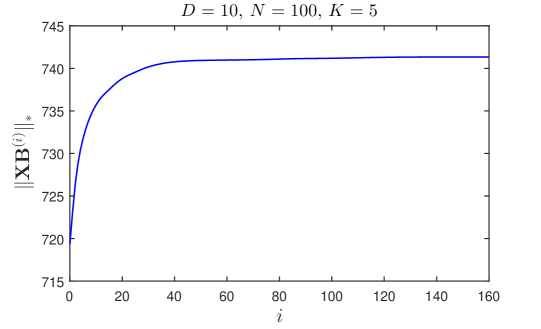
Figure 4: The objective metric of (19), versus the iteration index $i$ for Algorithm 1 (single realization; $D=10$, $N=100$, $K=5$).

The convergence of Algorithm 1 was formally proven in the previous Section. At this point, to visualize the convergence, we fix $D=10$, $N=100$, and $K=5$, and generate $\mathbf{X}\in\mathbb{R}^{D\times N}$ with entries drawn independently from $\mathcal{CN}(0,1)$. Then, we run on $\mathbf{X}$ Algorithm 1 (initialized at arbitrary $\mathbf{B}^{(0)}$) and plot in Fig. 4 $\|\mathbf{X}\mathbf{B}^{(i)}\|_{*}$ versus the iteration index $i$. We observe that, indeed, the objective nuclear-norm-maximization metric increases monotonically.

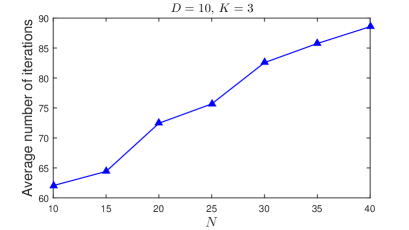
Figure 5: Average number of iterations needed for the convergence of Algorithm 1, versus the number of data points $N$ ($1000$ realizations; $D=10$, $K=3$).

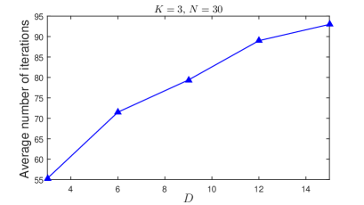
Figure 6: Average number of iterations needed for the convergence of Algorithm 1, versus the number of data points $N$ ($1000$ realizations; $K=3$, $N=30$).

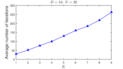
Figure 7: Average number of iterations needed for the convergence of Algorithm 1, versus the number of data points $N$ ($1000$ realizations; $D=10$, $N=20$).

Next, we wish to examine the number of iterations needed for Algorithm 1 to converge, especially as the problem-size parameters $D$, $N$, and $K$ take different values. First, we set $D=10$ and $K=3$ and vary $N=10,15,\ldots,40$. We draw again the entries of $\mathbf{X}$ independently from $\mathcal{CN}(0,1)$ and plot in Fig. 5 the average number of iterations needed for Algorithm 1 to converge (averaging is conducted over 1000 independent realizations of $\mathbf{X}$) . We observe that, expectedly, the number of iterations increases along $N$. However, importantly, it appears to increase sub-linearly in $N$. In Fig. 6 fix $K=3$ and $N=30$ and plot the average number of iterations needed for convergence versus $D$; in Fig. 7 we fix $D=10$ and $N=20$ and plot the average number of iterations versus $K$. We observe that the number of iterations increases sub-sub-linearly along $D$ and rather linearly along $K$.

IV.B Subspace Calculation

In this first experiment, we investigate and compare the outlier resistance of L2-PCA and L1-PCA. We consider the data matrix $\mathbf{X}$ of (59), consisting of $N=10$ data points of size $D=5$. A data processor wants to calculate the $(K=3)$-dimensional dominant subspace of $\mathbf{X}$, spanned by its $K$ highest-singular-value left singular-vectors in $\mathbf{Q}_{n}\in\mathbb{C}^{D\times K}$. However, unexpectedly, 1 out of the $N=10$ measurements (say, the first one) has been additively corrupted by a random point $\mathbf{c}$ drawn from $\mathcal{CN}(\mathbf{0}_{D},\sigma^{2}\mathbf{I}_{D})$. Therefore, instead of $\mathbf{X}$, what is available is the corrupted counterpart $\mathbf{X}_{cor}=[\mathbf{x}_{1}+\mathbf{c},\mathbf{x}_{2},\ldots,\mathbf{x}_{N}]$ (the data processor is not aware of the corruption). Instead of the nominal, sought-after $\text{span}(\mathbf{Q}_{n})$, the data processor calculates the span of the $K$ L2-PCs of $\mathbf{X}_{cor}$, $\mathbf{Q}_{L2}$, and the span of the $K$ L1-PCs of $\mathbf{X}_{cor}$, $\mathbf{Q}_{L1}$. To quantify the corruption-resistance of the two subspace calculators, we measure the subspace proximity (SP)

$$\text{SP}(\mathbf{Q},\mathbf{Q}_{n})=\frac{1}{\sqrt{K}}\|\mathbf{Q}_{n}^{H}\mathbf{Q}\|_{2}\in[0,1],$$ (58)

for $\mathbf{Q}=\mathbf{Q}_{L2}$ and $\mathbf{Q}=\mathbf{Q}_{L1}$. Certainly, if $\text{span}(\mathbf{Q})$ is orthogonal to the sought-after $\text{span}(\mathbf{Q}_{n})$, then $\mathbf{Q}^{H}\mathbf{Q}_{n}=\mathbf{0}_{K\times K}$ and $\text{SP}(\mathbf{Q},\mathbf{Q}_{n})=0$. On the other hand, if-and-only-if $\text{span}(\mathbf{Q})$ coincides with $\text{span}(\mathbf{Q}_{n})$, then $\text{SP}(\mathbf{Q},\mathbf{Q}_{n})=1$.

$$\mathbf{X}=\begin{bmatrix}-0.3003-i~{}1.0117&0.4618+i~{}0.0705&-0.3924-i~{}0.1602&-0.5327+i~{}0.1129&1.9368-i~{}0.5685\\ -0.3886-i~{}0.6530&-0.6204-i~{}0.3556&0.7040-i~{}1.3574&0.3315+i~{}0.9675&-1.5390-i~{}0.8711\\ -0.5961+i~{}0.1708&0.6005-i~{}1.8511&-0.5541-i~{}0.6086&-0.4701+i~{}0.3234&1.0896+i~{}1.3071\\ -0.0893+i~{}0.1863&-0.6031+i~{}0.3869&-0.7038+i~{}0.0123&1.0782+i~{}1.4440&0.9593-i~{}0.9096\\ -0.1678+i~{}1.7097&0.5883-i~{}0.7234&-0.5185-i~{}0.2924&-0.3291-i~{}1.7799&-1.1252-i~{}0.5569\\ 0.2485+i~{}0.6433&-1.3913-i~{}1.7947&0.1189+i~{}0.1334&0.0509-i~{}0.1326&-1.2163+i~{}0.4921\\ 0.5302-i~{}0.1632&-0.9533-i~{}0.3757&1.4074-i~{}1.2147&-0.4419+i~{}0.8734&-0.8092-i~{}0.6724\\ 0.0428+i~{}0.6675&-1.1010+i~{}0.6750&0.6385-i~{}0.7620&0.4554+i~{}0.5840&-0.7863+i~{}1.2148\\ -1.3608+i~{}0.5011&1.0467-i~{}0.1282&0.5043+i~{}0.1808&0.2366-i~{}0.8010&0.0459-i~{}0.3441\\ 0.5409-i~{}0.7822&0.0075-i~{}1.5285&1.4829+i~{}0.9075&-0.5216-i~{}0.0030&0.8504+i~{}0.8860\\ \end{bmatrix}^{T}.$$ (59)

 

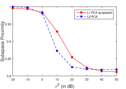
Figure 8: Subspace proximity versus corruption variance $\sigma^{2}$, for L2-PCA and L1-PCA ($10~{}000$ realizations; $D=5$, $N=10$, $K=2$).

In Fig. 8 we plot the average SP (over $10~{}000$ independent corruption realizations) for L2-PCA and L1-PCA versus the corruption variance $\sigma^{2}$. We observe that for weak corruption of variance $\sigma^{2}<0$dB, L1-PCA and L2-PCA exhibit almost identical performance, with SP approaching the ideal value of $1$. We also notice that for very strong corruption of variance $\sigma^{2}>35$dB, both L1-PCA and L2-PCA get similarly misled converging to a minimum SP of about $0.82$. Interestingly, for all intermediate values of $\sigma^{2}$, L1-PCA exhibits significantly superior performance in calculating the nominal subspace. For example, for $\sigma^{2}=10$dB, L1-PCA attains $93\%$ SP, while L2-PCA attains $87\%$ SP.

IV.C Cognitive Signature Design

Next, we investigate an application example for complex L1-PCA, drawn from the field of wireless communications. We consider a system of $K$ single-antenna primary sources using unknown complex-valued spread-spectrum signatures of length $L$ chips. The signatures of the $K$ sources are linearly independent (possibly, orthogonal), so that they do not interfere with each-other, spanning a $K$-dimensional subspace in $\mathbb{C}^{L}$. We consider now that $L-K$ secondary sources wish also to attempt using the channel, using length-$L$ spread spectrum signatures. Of course, the secondary sources should not interfere with the primary ones; for that reason, the $L-K$ signatures of the secondary sources should be orthogonal to the $K$ signatures of the primary sources –i.e., the secondary sources should transmit in the nullspace of the primary ones. Therefore, the secondary users wish to estimate the subspace spanned by the primary signatures and then design signatures in its orthogonal complement.

IV.C1 Training Phase

With this goal in mind, we consider a collection of $N$ snapshots that correspond to primary transmissions in the presence of additive white Gaussian noise (AWGN); these snapshots will be used for estimating the primary-source signature subspace (and then design secondary signatures in its orthogonal complement). To make the problem more challenging, we consider that while these snapshots are collected, an unexpected, strong interference source is also sporadically active. That is, the $n$-th recorded snapshot vector (after down-conversion and pulse-matching), $\mathbf{x}(n)\in\mathbb{C}^{L}$, has the form

$$\mathbf{x}(n)=\underbrace{\sum_{k=1}^{K}\mathbf{s}_{k}y_{k}(n)+\mathbf{n}(n)}_{\text{nominal}}+\underbrace{\gamma(n)\mathbf{i}(n)}_{\begin{smallmatrix}\text{unexpected}\\ \text{corruption}\end{smallmatrix}}\in\mathbb{C}^{L\times 1}.$$ (60)

In (60), $y_{k}(n)$ accounts for the product of the $n$-th power-scaled information symbol transmitted by the $k$-th primary source with the flat-fading channel between the $k$-th source and the receiver, with $E\{|y_{k}(n)|^{2}\}=1$; $\mathbf{s}_{k}\in\mathbb{C}^{L}$ is the signature of the $k$-th primary source, designed such that $\|\mathbf{s}_{k}\|_{2}=1$ and $\mathbf{s}_{k}^{H}\mathbf{s}_{l}=0$, for $k\neq l$; $\mathbf{n}(n)$ is additive white Gaussian noise (AWGN), drawn from $\mathcal{CN}\left(\mathbf{0}_{L\times 1},\frac{1}{L}\mathbf{I}_{L}\right)$; and $\mathbf{i}(n)$ accounts for unexpected sporadic interference, drawn from $\mathcal{CN}\left(\mathbf{0}_{L\times 1},\frac{100}{L}\mathbf{I}_{L}\right)$. $\{\gamma(n)\}_{n=1}^{N}$ are independent and identically distributed (i.i.d.) $\{0,1\}$-Bernoulli($\epsilon$) variables that indicate interference activity. That is, each snapshot is corrupted by an unexpected interference signal with probability $\epsilon$. According to the chosen values of symbol and noise variance, the primary users operate at signal-to-noise ratio (SNR) of $0$dB. The recorded snapshots are organized in the complex data record $\mathbf{X}\triangleq[\mathbf{x}(1),\mathbf{x}(2),\dots\mathbf{x}(N)]\in\mathbb{C}^{L\times N}.$ Then, we analyze $\mathbf{X}$ to estimate the $K$-dimensional primary-source transmission subspace, $\mathcal{S}\triangleq\mathrm{span}([\mathbf{s}_{1},$ $\mathbf{s}_{2},\ldots,\mathbf{s}_{K}])$. Traditionally, $\mathcal{S}$ would be estimated as the span of $\mathbf{Q}_{L2}=\underset{\mathbf{Q}\in\mathbb{C}^{L\times K};~{}\mathbf{Q}^{H}\mathbf{Q}=\mathbf{I}_{K}}{\text{argmax}}{\|\mathbf{X}^{H}\mathbf{Q}\|_{2}}.$ The reason is that, if all snapshots are nominal (i.e., no unexpected impulsive interference), as $N$ tends to infinity the span of $\mathbf{Q}_{L2}$ provably coincides with that of the $K$ dominant eigenvectors of the snapshot autocorrelation matrix $E\{\mathbf{x}(n)\mathbf{x}(n)^{H}\}$, which, in turn, coincides with $\mathcal{S}$. To examine the performance of complex L1-PCA, in this experiment we also estimate $\mathcal{S}$ by the span of $\mathbf{Q}_{L1}=\underset{\mathbf{Q}\in\mathbb{C}^{L\times K};~{}\mathbf{Q}^{H}\mathbf{Q}=\mathbf{I}_{K}}{\text{argmax}}{\|\mathbf{X}^{H}\mathbf{Q}\|_{1}}.$ After $\mathcal{S}$ is estimated, we pick $L-K$ orthogonal secondary signatures from the orthogonal complement of $\text{span}(\mathbf{Q}_{L2})$ (or $\text{span}(\mathbf{Q}_{L1})$). The secondary users employ these signatures and conduct transmissions concurrently with the primary sources.

IV.C2 Concurrent Operation of Primary and Secondary Sources

At this point, the assume that the impulsive corruption that interfered with secondary-signature training is no longer active. As both the primary and secondary sources transmit, the receiver applies matched filtering for each primary source. To evaluate the ability of L2/L1-PCA to identify the actual primary-source subspace (and thus enable secondary signatures that do not interfere with the primary sources), we measure and plot the post-filtering signal-to-interference-plus-noise ratio (SINR) for the primary users. It is expected that if $\text{span}(\mathbf{Q}_{L2})$ (or $\text{span}(\mathbf{Q}_{L1})$) is close to $\mathcal{S}$, then the interference of the secondary-sources to the primary sources will be minimized and, accordingly, the aggregate post-matched-filtering SINR (sum-SINR) of all $K$ primary sources will be high. We denote by $\mathbf{s}_{l}^{\prime}$ the signature of the $k$-th secondary source. It holds $\|\mathbf{s}_{l}^{\prime}\|_{2}=1$ and $\mathbf{s}_{l}^{\prime H}\mathbf{s}_{k}=0$ for $k\neq l$. Also, we denote by $y_{k}^{\prime}(n)$ the $n$-th symbol/channel compound for the $k$-th secondary source, with $E\{|y_{k}^{\prime}(n)|^{2}\}=\rho^{2}$ for all $k$. Sum-SINR is formally defined as $\text{sum-SINR}=\sum_{k=1}^{K}\text{SINR}_{k}$, where

$$\text{SINR}_{k} \triangleq\frac{E\left\{\left|\mathbf{s}_{k}^{H}\mathbf{s}_{k}y_{k}(n)\right|^{2}\right\}}{E\left\{\left|\mathbf{s}_{k}^{H}\left(\sum_{m\neq k}\mathbf{s}_{m}y_{m}(n)+\sum_{l=1}^{L-K}\mathbf{s}_{l}^{\prime}y_{k}^{\prime}(n)+\mathbf{n}(n)\right)\right|^{2}\right\}}$$ (61)

$$=\frac{1}{1+\rho^{2}\left|\sum_{l=1}^{L-K}\mathbf{s}_{k}^{H}\mathbf{s}_{l}^{\prime}\right|^{2}}.$$ (62)

Certainly, sum-SINR is a decreasing function of the transmission energy of the secondary sources, $\rho^{2}$. We also observe that if $\mathcal{S}$ was perfectly estimated and, accordingly $\{\mathbf{s}_{k}^{\prime}\}_{k=1}^{L-K}$ were designed in its orthogonal complement, then $\mathbf{s}_{k}^{H}\mathbf{s}_{l}^{\prime}=0$ for all $k,l$ and (62) takes its maximum value $1$ (or $0$dB), independently of $\rho$.

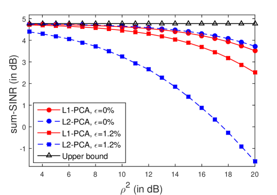
Figure 9: Post-filtering sum-SINR versus the transmission energy of the secondary sources, $\rho^{2}$ ($10~{}000$ realizations; $L=8$, $K=3$, $N=200$).

In our numerical simulation we set $N=200$, $L=8$, and $K=3$. In Fig. 9 we plot the average value of sum-SINR (calculated over $10~{}000$ independent experiments) versus $\rho^{2}$, for snapshot-corruption probability $\epsilon=0\%$ and $\epsilon=1.2\%$. As a benchmark, we also plot the horizontal line of $10\log_{10}(K)$ dB, which corresponds to the sum-SINR if $\mathcal{S}$ was accurately estimated (i.e., $\mathbf{s}_{k}^{H}\mathbf{s}_{l}^{\prime}=0$ for all $k,l$). We observe that if $\epsilon=0$ (i.e., all $N$ training snapshots nominal), L2-PCA-based and L1-PCA-based signature designs yield almost identical high sum-SINR performance. When however $\epsilon$ increases from $0$ to $1.2\%$, then L2-PCA gets significantly impacted; accordingly, the sum-SINR performance of the L2-PCA-based signature design diminishes significantly. On the other hand, we observe that the L1-PCA-based design exhibits sturdy robustness against the corruption of the training snapshots, maintaining high sum-SINR performance close to the nominal one.

IV.D Direction-of-Arrival Estimation

Direction-of-Arrival (DoA) estimation is a key operation in many applications, such as wireless node localization and network topology estimation. Super-resolution DoA estimation relies, traditionally, on the L2-PCA of a collection of –as, e.g., in MUltiple-SIgnal Classification (MUSIC) [44].

In this numerical study, we consider a receiver equipped with a uniform linear array (ULA) of $D$ antenna elements which receives signals from $K$ sources of interest located at angles $\Theta=\{\theta_{1},\theta_{2},\ldots,\theta_{K}\}$ with respect to the broadside. The inter-element spacing of the array, $d$, is fixed at half the wavelength of the received signal and the array response vector for a signal that arrives from angle $\phi\in[\frac{-\pi}{2},\frac{\pi}{2})$ is

$$\mathbf{s}(\phi)\triangleq[1,e^{-j\pi d\sin(\phi)},\ldots,e^{-j(D-1)\pi d\sin(\phi)}]^{T}\in\mathbb{C}^{D\times 1}.$$ (63)

To make the problem more challenging, we assume that apart from the $K$ sources of interest, there are also $J$ unexpected, sporadically interfering sources (jammers), impinging on the ULA from angles $\Theta^{\prime}=\{\theta_{1}^{\prime},\theta_{2}^{\prime},\ldots,\theta_{J}^{\prime}\}$. Therefore, the $n$th snapshot at the receiver is of the form

$$\mathbf{x}(n)=\underbrace{\sum_{k=1}^{K}\mathbf{s}({\theta_{k}})y_{k}(n)~{}~{}+\mathbf{n}(n)}_{\text{nominal}}+\underbrace{\sum_{j=1}^{J}\gamma_{n,j}\mathbf{s}({\theta_{j}}^{\prime})y_{j}^{\prime}(n)}_{\text{unexpected jamming}}\in\mathbb{C}^{D\times 1}.$$ (64)

In (64), $y_{k}(n)$ and $y_{k}(n)^{\prime}$ account for the compound symbol of the $k$-th source and $j$-th jammer, respectively; $\gamma_{n,j}$ is a $\{0,1\}$-Bernoulli($\epsilon$) activity indicator for jammer $j$ at snapshot $n$; $\mathbf{n}(n)$ is the AWGN component, drawn from $\mathcal{CN}(\mathbf{0}_{D},\sigma^{2}\mathbf{I}_{D})$.

The popular MUSIC DoA estimation method collects all $N$ snapshots in $\mathbf{X}=[\mathbf{x}(1),\mathbf{x}(2),\ldots,\mathbf{x}(N)]$ and calculates the source-signal subspace by the span of $\mathbf{Q}_{L2}=\underset{\mathbf{Q}\in\mathbb{C}^{D\times K};~{}\mathbf{Q}^{H}\mathbf{Q}=\mathbf{I}_{K}}{\text{argmax}}{\|\mathbf{X}^{H}\mathbf{Q}\|_{2}}.$ If all snapshots are nominal, as $N$ tends to infinity $\text{span}(\mathbf{Q}_{L2})$ tends to coincide with $\text{span}([\mathbf{s}(\theta_{1}),\ldots,\mathbf{s}(\theta_{K})])$ and allows for accurate DoA estimation, by identifying the $K$ peaks of the, so called, MUSIC spectrum

$$P(\phi;\mathbf{Q}_{L2})=\|(\mathbf{I}_{D}-\mathbf{Q}_{L2}\mathbf{Q}_{L2}^{H})\mathbf{s}(\phi)\|_{2}^{-1}.$$ (65)

In this work, we also conduct DoA estimation by finding the peaks of the L1-PCA spectrum $P(\phi;\mathbf{Q}_{L1})$, where $\mathbf{Q}_{L1}=\underset{\mathbf{Q}\in\mathbb{C}^{D\times K};~{}\mathbf{Q}^{H}\mathbf{Q}=\mathbf{I}_{K}}{\text{argmax}}{\|\mathbf{X}^{H}\mathbf{Q}\|_{1}}.$.

In this numerical study, we set $D=12$, $K=4$, $J=3$, source DoAs $\Theta=\{-40^{\circ},-21^{\circ},-7^{\circ},60^{\circ}\}$, and jammer DoAs $\Theta^{\prime}=\{0^{\circ},20^{\circ},80^{\circ}\}$. The number of snapshots available for DoA estimation (i.e., the columns of $\mathbf{X}$), $N$, vary from $10$ to $100$ with step $10$. The $K$ sources of interest operate at SNR 0dB; when active, jammers operate at the much higher SNR of 15dB. We conduct $10~{}000$ independent DoA estimation experiments and evaluate the average DoA estimation performance of the L2-PCA-based and L1-PCA-based methods by means of the standard root-mean-squared error (RMSE), defined as

$$\text{RMSE}\triangleq\sqrt{\frac{1}{10000}\sum_{m=1}^{10000}\sum_{k=1}^{K}|\theta_{k}-\hat{\theta}_{k}(m)|^{2}}$$ (66)

where $\hat{\theta_{k}}(m)$ is the estimate of $\theta_{k}$ at the $m$-th experiment.

In Fig. 10 we set $\epsilon=0$ (i.e., no unexpected jamming) and plot the RMSE for L2-PCA and L1-PCA versus the number of snapshots, $N$. We observe that L2-PCA and L1-PCA have almost identical RMSE performance, which improves towards $0^{\circ}$ as $N$ increases. Then, in Fig. 11 we increase $\epsilon$ to $2\%$. The performance of L2-PCA (standard MUSIC [44]) changes astoundingly. We observe that now the performance of MUSIC deteriorates as the sample-support $N$ increases converging on a plateau of poor performance at RMSE=$16^{\circ}$. On the other hand, quite interestingly, L1-PCA resists the directional corruption of the jammers and, as $N$ increases it attains decreasing RMSE which reaches as low as $3^{\circ}$ for $N=100$. That is, in contrast to L2-PCA, L1-PCA is benefited by an increased number of processed data points when the corruption ratio remains constant.

V Conclusions

We showed that, in contrast to the real-valued case, complex L1-PCA is formally $\mathcal{NP}$-hard in the number of data points. Then, we showed how complex L1-PCA can be cast and solved through a unimodular nuclear-norm maximization problem. We conducted optimality analysis and provided necessary conditions for global optimality. For the case of K = 1 principal component, we provided necessary and sufficient conditions for local optimality. Based on the optimality conditions, we presented the first two sub-optimal/iterative algorithms in the literature for L1-PCA. Finally, we presented extensive numerical studies from the fields of data analysis and wireless communications and showed that when the processed complex data are outlier-free, L1-PCA and L2-PCA perform very similarly. However, when the processed data are corrupted by faulty measurements L1-PCA exhibits sturdy resistance against corruption and significantly robustifies applications that rely on principal-component data feature extraction.

    Algorithm 1: Iterative complex L1-PCA for general $K\geq 1$ (mild condition)   Input: $\mathbf{X}\in\mathbb{C}^{D\times N}$;  $K<\text{rank}(\mathbf{X})$;  init. $\mathbf{B}$; $\delta>0$
1: $\alpha\leftarrow\|\mathbf{X}\mathbf{B}\|_{*}$ 3: while true 4:       $\mathbf{B}\leftarrow\mathrm{sgn}\left(\mathbf{X}^{H}\mathrm{unt}\left(\mathbf{X}\mathbf{B}\right)\right)$ 5:       if $\|\mathbf{X}\mathbf{B}\|_{*}-\alpha>\delta$, $\alpha\leftarrow\|\mathbf{X}\mathbf{B}\|_{*}$ 6:       else, break 7: $[\mathbf{U},\mathbf{S}_{K\times K},\mathbf{V}]\leftarrow\text{svd}(\mathbf{X}\mathbf{B})$ 8: $\mathbf{Q}\leftarrow\mathbf{U}\mathbf{V}^{H}$
Output: $\hat{\mathbf{Q}}_{L1}\leftarrow\mathbf{Q}$ and $\hat{\mathbf{B}}\leftarrow\mathbf{B}$    

Figure 2: Proposed Algorithm 1 for the L1-PCA of $\mathbf{X}\in\mathbb{C}^{D\times N}$ (general $K\geq 1$). The algorithm relies on the mild optimality condition in (29).

    Algorithm 2: Iterative complex L1-PCA for $K=1$ (strong condition)   Input: $\mathbf{X}\in\mathbb{C}^{D\times N}$;  init. $\mathbf{b}$; $\delta>0$
1: $\mathbf{A}_{d}=\mathbf{X}^{H}\mathbf{X}-\text{Diag}([\|\mathbf{x}_{1}\|_{2}^{2},\ldots,\|\mathbf{x}_{N}\|_{2}^{2}]^{T})$,  $\alpha\leftarrow\|\mathbf{A}_{d}\mathbf{b}\|_{1}$ 3: while true 4:       $\mathbf{b}\leftarrow\mathrm{sgn}\left(\mathbf{A}_{d}\mathbf{b}\right)$ 5:       if $\|\mathbf{A}_{d}\mathbf{b}\|_{1}-\alpha>\delta$, $\alpha\leftarrow\|\mathbf{A}_{d}\mathbf{b}\|_{1}$ 6:       else, break 7: $\mathbf{q}\leftarrow\mathbf{X}\mathbf{b}\|\mathbf{X}\mathbf{b}\|_{2}^{-1}$
Output: $\hat{\mathbf{q}}_{L1}\leftarrow\mathbf{q}$ and $\hat{\mathbf{b}}\leftarrow\mathbf{b}$    

Figure 3: Proposed Algorithm 2 for calculation of the $K=1$ L1-PC of $\mathbf{X}\in\mathbb{C}^{D\times N}$. The algorithm relies on the strong optimality condition in (39).

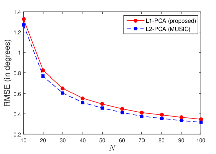
Figure 10: RMSE (in degrees) versus $N$, in nominal operation (no jammers; $\epsilon=0$), for L2-PCA (MUSIC method [44]) and L1-PCA ($10~{}000$ realizations; $D=12$, $\Theta=\{-40^{\circ},-21^{\circ},-7^{\circ},60^{\circ}\}$, and $\Theta^{\prime}=\{0^{\circ},20^{\circ},80^{\circ}\}$).

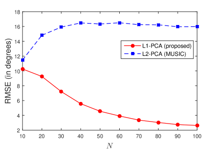
Figure 11: RMSE (in degrees) versus $N$, considering jammer corruption ($\epsilon=2\%$), for L2-PCA (MUSIC method [44]) and L1-PCA ($10~{}000$ realizations; $D=12$, $\Theta=\{-40^{\circ},-21^{\circ},-7^{\circ},60^{\circ}\}$, and $\Theta^{\prime}=\{0^{\circ},20^{\circ},80^{\circ}\}$).

References

- [1] N. Tsagkarakis, P. P. Markopoulos, D. A. Pados, “Direction finding by complex L1-principal component analysis,” in Proc. IEEE Int. Workshop Signal Process. Adv. Wireless Commun. (SPAWC), Stockholm, Sweden, Jun. 2015, pp. 475-479.
- [2] K. Pearson, “On lines and planes of closest fit to systems of points in space,” Philosoph. Mag., vol. 2, pp. 559–572, 1901.
- [3] C. Eckart and G. Young, “The approximation of one matrix by another of lower rank,” Phychomerika, vol. 1, pp. 211-218, Sep. 1936.
- [4] C. D. Meyer, Matrix analysis and applied linear algebra. Philadelphia, PA: Siam, 2000.
- [5] G. H. Golub and C. F. Van Loan, Matrix Computations, 3rd ed. Baltimore, MD: The Johns Hopkins Univ. Press, 1996.
- [6] M. Brand, “Fast low-rank modifications of the thin singular value decomposition,” Linear Algebra App., vol. 415, no. 1, pp. 20-30, May 2006.
- [7] N. Srebro and T. Jaakkola, “Weighted low-rank approximations,” in Proc. Int. Conf. Mach. Learn. (ICML), Washington DC, Aug. 2003, pp. 720-727.
- [8] P. Anandan and M. Irani, “Factorization with uncertainty.” Int. J. Comp. Vision, vol. 49, pp. 101-116, Sep. 2002.
- [9] F. De La Torre and M. Black, “A framework for robust subspace learning,” Int. J. Comp. Vision, vol. 54, pp. 117-142, Aug. 2003.
- [10] P. P. Markopoulos, G. N. Karystinos and D. A. Pados, “Optimal algorithms for L1-subspace signal processing,” IEEE Trans. Signal Proc., vol. 62, pp. 5046-5058, Oct. 2014.
- [11] P. P. Markopoulos, G. N. Karystinos and D. A. Pados, “Some options for L1-subspace singal processing,” Proc. Int. Symp. Wireless Commun. Syst. (ISWCS), Ilmenau, Germany, Aug., 2013, pp. 622-626.
- [12] S. Kundu, P. P. Markopoulos, and D. A. Pados, “Fast computation of the l1-principal component of real-valued data,” in Proc. IEEE Int. Conf. Acoust., Speech, Signal Process. (ICASSP), Florence, Italy, May 2014, pp. 8028-8032.
- [13] P. P. Markopoulos, S. Kundu, S. Chamadia, and D. A. Pados, “Efficient L1-norm Principal-Component Analysis via bit flipping,” IEEE Trans. Signal Process., vol. 65, pp. 4252-4264, Aug. 2017.
- [14] P. P. Markopoulos, S. Kundu, S. Chamadia, and D. A. Pados, “L1-norm Principal-Component Analysis via bit flipping,” in Proc. IEEE Int. Conf. Mach. Learn. App. (ICMLA), Anaheim, CA, Dec. 2016, pp. 326-332.
- [15] R. R. Singleton, “A method for minimizing the sum of absolute values of deviations,” Ann. Math. Stat., vol. 11, pp. 301-310, Sep. 1940.
- [16] I. Barrodale, “L1 approximation and the analysis of data,” J. Royal Stat. Soc., App. Stat., vol. 17, pp. 51-57, 1968.
- [17] Q. Ke and T. Kanade, “Robust subspace computation using L1 norm,” Internal Technical Report Computer Science Dept., Carnegie Mellon Univ., Pittsburgh, PA, CMU-CS-03172, Aug. 2003.
- [18] J. P. Brooks, J. H. Dula, and E. L. Boone, “A pure L1-norm principal component analysis,” J. Comput. Stat. Data Anal., vol. 61, pp. 83-98, May 2013.
- [19] N. Kwak, “Principal component analysis based on L1-norm maximization,” IEEE Trans. Patt. Anal. Mach. Intell., vol. 30, pp. 1672-1680, Sep. 2008.
- [20] F. Nie, H. Huang, C. Ding, D. Luo, and H. Wang, “Robust principal component analysis with non-greedy L1-norm, maximization,” in Proc. Int. Joint Conf. Artif. Intell. (IJCAI), Barcelona, Spain, Jul. 2011, pp. 1433-1438.
- [21] M. McCoy and J. A. Tropp, “Two proposals for robust PCA using semidefinite programming,” Electron. J. Stat., vol. 5, pp. 1123-1160, Jun. 2011.
- [22] A. Eriksson and A. v. d. Hengel, “Efficient computation of robust low-rank matrix approximations in the presence of missing data using the L1 norm,” in Proc. IEEE Conf. Comput. Vision Patt. Recogn. (CVPR), San Francisco, CA, Jun. 2010, pp. 771-778.
- [23] Y. Pang, X. Li, and Y. Yuan, “Robust tensor analysis with L1-norm,” IEEE Trans. Circuits Syst. Video Technol., vol. 20, pp. 172-178, Feb. 2010.
- [24] C. Ding, D. Zhou, X. He, and H. Zha, “-PCA: Rotational invariant L1-norm principal component analysis for robust subspace factorization,” in Proc. Int. Conf. Mach. Learn., Pittsburgh, PA, Jun. 2006, pp. 281-288.
- [25] P. P. Markopoulos, S. Kundu, and D. A. Pados, “L1-fusion: Robust linear-time image recovery from few severely corrupted copies,” in Proc. IEEE Int. Conf. Image Process. (ICIP), Quebec City, Canada, Sep. 2015, pp.1225-1229.
- [26] D. Meng, Q. Zhao, and Z. Xu, “Improve robustness of sparse PCA by L1-norm maximization,” Patt. Recogn., vol. 45, pp. 487-497, Jan. 2012.
- [27] M. Johnson and A. Savakis, “Fast L1-eigenfaces for robust face recognition,” in Proc. IEEE West. New York Image Signal Process. Workshop (WNYISPW), Rochester, NY, Nov. 2014, pp. 1-5.
- [28] P. P. Markopoulos, “Reduced-rank filtering on L1-norm subspaces,” in Proc. IEEE Sensor Array Multichan. Signal Process. Workshop (SAM), Rio de Janeiro, Brazil, pp. 1–5, Jul. 2016.
- [29] S. Chamadia and D. A. Pados, “Optimal sparse L1-norm Principal-Component analysis,” in Proc. Int. Conf. Acoust., Speech, Signal Process. (ICASSP), New Orleans, LA, March 2017, pp. 2686-2690.
- [30] F. Maritato, Y. Liu, S. Colonnese, and D. A. Pados, “Cloud-assisted individual l1-pca face recognition using wavelet-domain compressed images,” in Proc. Europ. Workshop Visual Inf. Process. (EUVIP), Marseilles, France, Oct. 2016, pp. 1-6.
- [31] F. Maritato, Y. Liu, S. Colonnese, and D. A. Pados, “Face recognition with L1-norm subspaces,” in Proc. SPIE Def. Commerc. Sens. (SPIE DCS), Baltimore, MD, Apr. 2016, pp. 98570K-1–98570K-8.
- [32] M. Pierantozzi, Y. Liu. D. A. Pados, and S. Colonnese, “Video background tracking and foreground extraction via L1-subspace updates,” in Proc. SPIE Def. Commerc. Sens. (SPIE DCS), Baltimore, MD, Apr. 2015, pp. 985708-1–985708-16.
- [33] Y. Liu and D. A. Pados, “Compressed-sensed-domain L1-PCA video surveillance,” IEEE Trans. Multimedia, vol 18, pp. 351-63, Mar. 2016.
- [34] N. Tsagkarakis, P. P. Markopoulos, and D. A. Pados, “On the L1-norm approximation of a matrix by another of lower rank,” in Proc. IEEE Int. Conf. Mach. Learn. App. (ICMLA), Anaheim, CA, Dec. 2016, pp. 768-773.
- [35] P. P. Markopoulos and F. Ahmad, “Indoor human motion classification by L1-norm subspaces of micro-Doppler signatures,” in Proc. IEEE Radar Conference (Radarcon), Seattle, WA, May 2017, pp. 1807-1810.
- [36] P. P. Markopoulos, D. A. Pados, G. N. Karystinos, and M. Langberg, “L1-norm principal-component analysis in L2-norm-reduced-rank data subspaces,” in Proc. SPIE Def. Commerc. Sens. (SPIE DCS), Anaheim, CA, Apr. 2017, pp. 1021104-1–1021104-10.
- [37] D. G. Chachlakis, P. P. Markopoulos, R. J. Muchhala, and A. Savakis, “Visual tracking with L1-Grassmann manifold modeling,” in Proc. SPIE Def. Commerc. Sens. (SPIE DCS), Anaheim, CA, Apr. 2017, pp. 1021102-1–1021102-12.
- [38] P. P. Markopoulos, N. Tsagkarakis, D. A. Pados, and G. N. Karystinos, “Direction finding with L1-norm subspaces,” in Proc. SPIE Def., Security, Sens. (SPIE DSS), Baltimore, MD, May 2014, pp. 91090J-1–91090J-11.
- [39] P. H. Schönemann, “A generalized solution of the orthogonal procrustes problem,” Psychometrika, vol. 31, pp. 1-10, Mar. 1966.
- [40] N. J. Higham, “Computing the Polar Decomposition-With Applications,” SIAM J. Sci. Stat. Comp., vol .7, pp. 1160-1174, Oct. 1986.
- [41] M. Soltanalian and P. Stoica, “Designing unimodular codes via quadratic optimization,” IEEE Trans. Signal Process., vol. 62, pp. 1221-1234, Mar. 2014.
- [42] G. N. Karystinos and A. P. Liavas, “Efficient computation of the binary vector that maximizes a rank-deficient quadratic form,” IEEE Trans. Inf. Theory, vol. 56, pp. 3581-3593, Jul. 2010.
- [43] P. M. Pardalos and S. A. Vavasis, “Quadratic programming with one negative eigenvalue is NP-Hard,” J. Global Optim., vol. 1, pp. 15-22, Feb. 1991.
- [44] R. O. Schmidt, “Multiple emitter location and signal parameter estimation,” IEEE Trans. Antennas and Propag., vol. 34, pp. 276-280, Mar. 1986.