A Monte Carlo Radiation Transfer Study of Photospheric Emission in Gamma Ray Bursts

Abstract

We present the analysis of photospheric emission for a set of hydrodynamic simulations of long duration gamma-ray burst jets from massive compact stars. The results are obtained by using the Monte Carlo Radiation Transfer code (MCRaT) to simulate thermal photons scattering through the collimated outflows. MCRaT allows us to study explicitly the time evolution of the photosphere within the photospheric region, as well as the gradual decoupling of the photon and matter counterparts of the jet. The results of the radiation transfer simulations are also used to construct light curves and time resolved spectra at various viewing angles, which are then used to make comparisons with observed data, and outline the agreement and strain points between the photospheric model and long duration gamma-ray burst observations. We find that our fitted time resolved spectral Band $\beta$ parameters are in agreement with observations, even though we do not consider the effects of non-thermal particles. Finally, the results are found to be consistent with the Yonetoku correlation, but bear some strain with the Amati correlation.

1. Introduction

Long duration Gamma Ray Bursts (LGRBs) are some of the most energetic events in the universe, emitting up to $10^{53}$ ergs of energy in the first few tens of seconds Kulkarni et al. (1999). The progenitors for these events are core collapse supernovae where the collapse of the iron core into a supermassive object causes a relativistic jet to form and flow through, and out of, the collapsing star. The prompt emission that is produced by the jet can be explained by the synchrotron shock model (SSM) (Rees & Meszaros, 1994) and the photospheric emission model (Rees & Mészáros, 2005).

SSM considers the radiation that is produced by shells of varying speeds colliding with one another outside of the photosphere. These collisions cause magnetic fields and non-thermal particles to form which then produce the radiation. This model is able to describe various observations of LGRBs such as the non-thermal spectrum and the light curve variability; however, the SSM is in tension with various observational relations such as the Amati, Yonetoku and Golenetskii Correlations (Amati, L. et al., 2002; Yonetoku et al., 2004; Golenetskii et al., 1983) as well as the spectral indicies of the observed LGRB spectra (Preece et al., 2002).

The photospheric model describes the radiation that is produced deep in the jet, where the opacity is extremely high. The radiation interacts heavily with the matter in the jet which affects the spectrum more than the process that initially creates the radiation. The trapped radiation is then released when the jet becomes transparent to the radiation propagating through it. The photospheric model is unable to naturally form a spectrum with non-thermal low and high energy tails; however, the idea of the fuzzy photosphere (Pe’er, 2008; Beloborodov, 2010) and sub-photospheric dissipation can cure the model’s inability to form a non-thermal high energy tail (Chhotray & Lazzati, 2015). Vurm & Beloborodov (2016) also showed that inclusion of a variety of dissipation mechanisms can produce the observationally expected non-thermal low energy tail, although this has yet to be shown when considering a realistic GRB jet. Opposing the SSM, a resounding success of the photospheric model is the model’s ability to reproduce all the observational correlations (López-Cámara et al., 2014; Lazzati et al., 2013a).

Previous studies of the photospheric model have considered highly detailed jet structures but assumed that the radiation and matter are perfectly coupled until the photosphere, whereafter the two components of the jet no longer interact with one another (Lazzati et al., 2009). Alternatively, other studies have considered rigorous radiation transfer calculations on simplified analytical outflows (Ito et al., 2013, 2014; Lundman et al., 2013, 2014; Vurm & Beloborodov, 2016).

The bridge between complex jet structures and self consistent radiation treatments has started to be built with Ito et al.’s (2015) investigation into the radiation signature of a precessing jet with the use of a Monte Carlo treatment of the radiation propagating through the jet. Lazzati (2016) then proposed an independent algorithm, called MCRaT, which was tested on spherical and cylindrical outflows and then applied to a single 2D LGRB simulation.

This paper continues along that path and presents the results of the MCRaT code on an ensemble of special relativistic hydrodynamical simulations of LGRBs and what the implications are for understanding these phenomena using the photospheric model (Lazzati, 2016). This paper is structured such that section 2 outlines the methods used in the analysis of the MCRaT data, section 3 discusses the results, and section 4 summarizes and discusses the implications of the results with theory and observations.

2. Methods

As described in Lazzati (2016), MCRaT loads a frame of a FLASH simulation and injects photons at an optical depth of $\sim 100$. The code then propagates and Compton scatters each photon until the last FLASH frame is reached. At this point, the code will restart by injecting photons into the next frame from which the last set of photons were injected. There are a total of $\sim 2.4\times 10^{5}$ photons in each simulation analyzed in this paper.

Once MCRaT has completed its run for a given hydrodynamical GRB simulation, the results can be used to construct theoretical light curves and time resolved spectra, much like what may be observed by FERMI (Yu, Hoi-Fung et al., 2016). To this aim, we insert a virtual detector at a suitable distance from the central engine and collect incoming photons registering their arrival time and frequency. From the calculated light curves and spectra, the MCRaT runs can then be compared to individual bursts or to observational trends such as the Yonetoku and Amati correlations (Yonetoku et al., 2004; Amati, L. et al., 2002). Any photon that propagates past the location of the virtual detector at the end of the radiation transfer simulation is collected and analyzed to produce light curves and time resolved spectra. From the 4-momenta, each photon’s direction of propagation and energy can be calculated. The propagation direction allows for the identification of which photons would be observed at a given angle relative to the GRB jet axis. Since each photon travels along a specific direction, we must specify a range of angles within which we collect the photons. Throughout this paper we will specify the average of the acceptance angle range as the viewing angle, $\theta_{\text{v}}$, and will consistently use a $\pm 0.5^{\circ}$ acceptance range; for example, a viewing angle of $1^{\circ}$ implies that all photons within $0.5^{\circ}$, inclusive, and $1.5^{\circ}$, exclusive, have been collected.

The detection time, $t_{\text{detect}}$, for any photon that propagates past the location of the virtual detector at the end of the radiation transfer simulation depends on the detected jet launching time $t_{\text{j}}$, the lab time at which the detection is evaluated $t_{\text{real}}$, and the photon displacement time $t_{\text{p}}$, i.e., the amount of time the photon has traveled past the detector:

$$t_{\text{detect}}=t_{\text{real}}-t_{\text{j}}-t_{p}$$ (1)

To compute the detected jet launching time $t_{\text{j}}$, we consider a virtual photon being emitted by the central engine at the time when the jet is launched. This virtual photon is detected by the virtual detector at $t_{\text{j}}=r_{\text{d}}/c$ which depends on the virtual detector’s distance from the central engine $r_{\text{d}}$. In order to know where to place the virtual detector, we must be able to identify the location of the photosphere for each viewing angle. To do this, we follow the method of Lazzati (2016) to obtain a plot of matter and photon temperature versus radial position from the jet. In each FLASH frame, for a given set of photons, binned by detection time, we calculate the average photon temperature and then identify the FLASH grid points nearest to each photon and calculate the average of the temperatures at each FLASH grid point. The temperature of the photon in the fluid frame, $T_{\mathrm{ph}}$, is calculated as

$$T_{\mathrm{ph}}=\frac{h\nu}{3k}$$ (2)

where h is Planck’s constant, $\nu$ is the photon comoving frequency, $k$ is the Boltzmann constant, and the factor of 3 comes from the photons being in Wien equilibrium with the matter (Beloborodov, 2013). The fluid frame temperature of the matter in the FLASH simulation grid, $T_{\mathrm{m}}$, is calculated as

$$T_{\mathrm{m}}=\big{(}\frac{3p}{a}\big{)}^{\frac{1}{4}}$$ (3)

where $p$ is the pressure, and $a$ is the radiation density constant. This equation conforms with the assumption in the FLASH hydrodynamic simulations that the adiabatic index of the fluid is $4/3$; this assumption becomes an approximation either when the fluid temperature is non-relativistic or the radiation is not a blackbody.

The plot of temperature versus radius, as discussed in section 3, ideally, shows the average photon temperature in the fluid frame approaching an asymptotic temperature. The distance at which the average photon temperature remains constant is where the edge of the photospheric region lies, and the virtual detector should be placed at this distance or at a larger one. In practice, since this distance is time dependent, we place our detector at the largest value for each viewing geometry.

Once the detection time and angle are calculated for each photon, the light curve can be constructed by collecting the photons that propagate within a given angle range, corresponding to $\theta_{\text{v}}\pm 0.5^{\circ}$, and then binned into 1 second bins, based on the arrival time of the photon. To convert the light curve from counts to luminosity the sum of the photons’ weights times energies are calculated. The weights are determined following equation 1 in Lazzati (2016).

The time resolved spectra are obtained by binning the observed photons, within a time interval of 1 second, into energy bins of logarithmically increasing widths. The number of photons collected in an energy bin can be converted into intensity by summing up each photon’s weight times energy and then dividing by the bin width.

The uncertainty for each point in the spectrum is derived assuming a Poisson distribution of counts. This makes the error associated with an energy bin the intensity at that energy bin divided by the square root of the number of photons collected in the energy bin. In order to perform a $\chi^{2}$ minimization to do a spectral fit, we only fit the energy bins that have at least 10 photons. We fit a Band function (Band et al., 1993) to the time resolved spectra in order to derive: the low and high energy spectral indices, $\alpha$ and $\beta$, and the peak energy, $E_{pk}=E_{o}(2+\alpha)$, where $E_{o}$ is the break energy. This is the definition used in Amati, L. et al. (2002) and Yu, Hoi-Fung et al. (2016). On the other hand, spectra can also be fit by the simpler comptonized (COMP) spectrum model (Yu, Hoi-Fung et al. (2016); Goldstein et al. (2013)). This is the model in which the Band function’s $\beta\rightarrow-\infty$.

In order to determine which function is statistically significant in fitting the data, we conduct an F-test. If the resulting p-value of the F-test is less than 5% – the conventional false positive acceptance rate – the Band function, with an extra free parameter, provides a statistically superior fit and is used. If the p-value is greater than 5%, then the simpler COMP fit is utilized to fit the spectrum. Furthermore, spectra where the fitted values of $\alpha$, $\beta$, and $E_{pk}$ were not well constrained were excluded from the analysis.

3. Results

Table 1Simulation Set Parameters

Simulation Name	Progenitor	Jet Luminosity (erg/s)	$\Gamma_{\infty}$
16OI	16OI	$5.33\times 10^{50}$	400
35OB	35OB	$5.33\times 10^{50}$	400
16TI	16TI	$5.33\times 10^{50}$	400
16TI.e150	16TI	$1\times 10^{50}$	400
16TI.e150.g100	16TI	$1\times 10^{50}$	100

In this section we present the results obtained by running MCRaT on various FLASH simulations of relativistic jets from several LGRB progenitor from Woosley & Heger (2006). These are the same simulations used by Lazzati et al. (2013a). They have a jet injection radius of $1\times 10^{9}$ cm, an initial lorentz factor of 5, an opening angle of $10^{\circ}$, and the engine was turned on for 100 s. The differences among the simulations are outlined in Table 1. The MCRaT simulations were run for at least 50 simulation seconds.

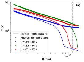
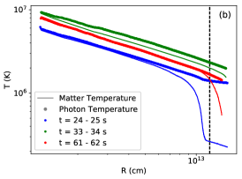
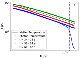
Figure 1.— Radiation and matter temperatures in the fluid frame as a function of distance from the central engine for the 35OB progenitor at viewing angles of $1^{\circ}$, $2^{\circ}$ and $3^{\circ}$, for figures (a), (b), and (c) respectively. The various colors represent photons which have been detected at different times. The circle markers represent the average photon temperature and the line is the average temperature of the FLASH grid points nearest to the photons of interest. The vertical dashed black line represents the location of the virtual detector at $1.2\times 10^{13}$ cm.

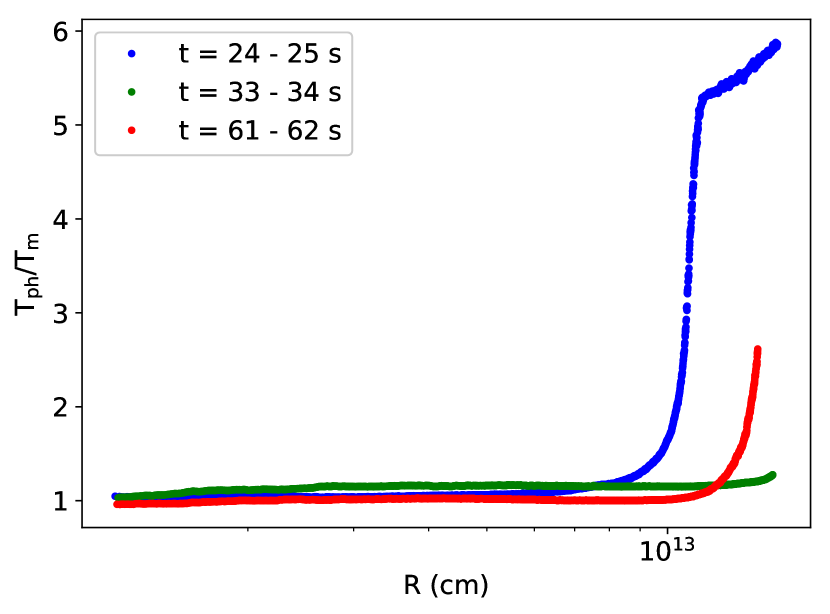
Figure 2.— The ratio of the comoving photon temperature, $T_{\mathrm{ph}}$, to the comoving matter temperature, $T_{\mathrm{m}}$, is plotted for photons detected at differing times since the jet launch as shown in Figure 1(b). The ratios begin to increase as the photons decouple from the jet. As such, each of the times show a different divergence point.

3.1. Decoupling of the Photons and the Matter

As described above, we use the comparison between the plasma and radiation temperatures to determine where the virtual detector needs to be placed. The plasma temperatures are read directly from the FLASH simulations, while the radiation temperature is computed by MCRaT.

Figure 1 shows the average fluid frame photon and matter temperatures as a function of distance from the central engine for the 35OB simulation at various viewing angles. For all the curves shown, the photons and matter start out coupled. However, the coupling drastically changes as the temperatures of the photon and matter begin to diverge from one another. While the matter continues in its cooling behavior, the photons cooling slows as the Compton coupling between matter and radiation weakens. Only when the decoupling becomes complete does the temperature of the photons becomes constant. Notice how the photons stay coupled to the matter for a larger distance at high viewing angles. This can be understood as due to the baryon entrainment in the jet along the boundary. Baryon entrainment increases opacity by both increasing the density of electrons and by reducing the Lorentz factor.

Each sub figure in Figure 1 shows that the photosphere is not a static surface in space, but rather an evolving surface that can vary quite dramatically. Between the three times shown for each of the viewing angles, the photosphere moves from being within the domain of our simulation at $t=3$s, to being out of the domain of our simulation at $t=30$s, and back to being relatively far back in the jet at $t=50$s. Hence, we refer to this region in which the photosphere moves as the “photospheric region”. In the small temporal and spatial domain of the simulations, we do not definitively reach the edge of the photospheric region at high viewing angles, $\theta_{\text{v}}\geq 3^{\circ}$. This effect is caused by the higher densities at $\theta_{\text{v}}\geq 3^{\circ}$, compared to the densities at angles closer to the jet axis. As a result of not reaching the photosphere for some populations of photons, our energies should be taken as an upper limit for the cases of high viewing angle. In order to get to the photosphere at high viewing angles, we would need to run FLASH simulations of larger domain. These, however, can be carried out only at the price of reducing the resolution (e.g., Ito et al. (2015)).

The changing location of the photosphere for a given GRB simulation is also shown in Figure 2, where the ratios are plotted for the three time periods shown in Figure 1b at a viewing angle of $2^{\circ}$. Each curve begins to turn away from a ratio of 1 at a different distance, indicative of the fact that the jet and the matter decouple at different distances for different times within the simulated jet. These characteristics of the temperature plots are consistent for all the simulations in our set.

3.2. Light Curves and $E_{pk}$

Figure 3 show synthetic, time-resolved light curves and spectra of the 16OI, 35OB, and 16TI.e150.g100 simulations for various viewing angles (see Table 1 for the details of the simulations inputs). The top plots show the light curve as a black line as well as the fitted peak energy as green markers with error bars, as measured in a 1 second time bin. The bottom plots show the temporal evolution of the fitted function parameters, where the low energy parameter, $\alpha$, is in red and the high energy Band parameter, $\beta$, is in blue. Many of the time resolved spectra were satisfactorily fitted with COMP spectra, and are shown in solid markers; other spectra were fitted with the Band function, if shown to be statistically significant with an F-test, and are shown with open markers.

The light curves are different from one simulation to the next, as well as from one viewing angle to another within the same FLASH simulation. The light curves exhibit diversity in their structure as well as in the tracking between the fitted peak energy and the light curve (or lack thereof). There are light curves for viewers at relatively high viewing angles where a global hard-to-soft trend of $E_{pk}$ is observed throughout the entire burst, while there are other cases in which the peak energy tracks the light curve. Other light curves do not display any clear hard-to-soft or tracking behavior. These results are qualitatively analogous to the observations made by FERMI (see Figure 6 in Yu, Hoi-Fung et al. (2016)).

In most cases, we see that viewing angles close to the jet axis, $\theta_{\text{v}}=1^{\circ}-2^{\circ}$, exhibit either a global hard-to-soft trend or a lack of an obvious trend. At higher viewing angles $\theta_{\text{v}}=3^{\circ}$, we typically see a tracking behavior.

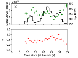
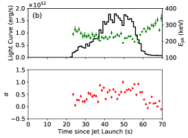
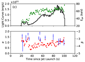
Figure 3.— Light curves from various simulations and viewing angles. Figure (a) shows the light curve of the 16OI progenitor at $\theta_{\text{v}}=1^{\circ}$, figure (b) shows the 35OB progenitor at $\theta_{\text{v}}=1^{\circ}$, and figure (c) shows the 16TI.e150.g100 light curve at $\theta_{\text{v}}=3^{\circ}$. These plots show how the various simulations can reproduce: a hard-to-soft tracking of $E_{pk}$, in (a), an anti-correlation between the luminosity and $E_{pk}$, in (b), and tracking between the $E_{pk}$ and the luminosity, as shown in (c).

3.3. Analysis of the Spectral Fits

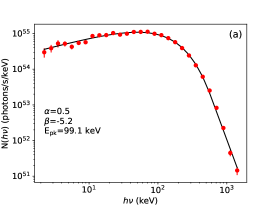
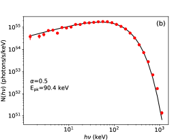
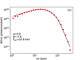
Figure 4.— Plots (a), (b) and (c) show the time-integrated spectra of the 16OI, 35OB, and 16TI.e150.g100 simulations respectively. The viewing angles for each simulation are the same as in Figure 3. The best fit parameters for each spectra are included on each plot. The 16OI and 16TI.e150.g100 spectra are best fit with a Band spectrum and the 35OB spectrum is best fit with a COMP spectrum.

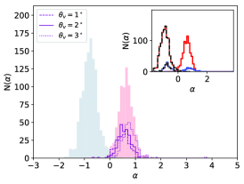
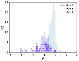
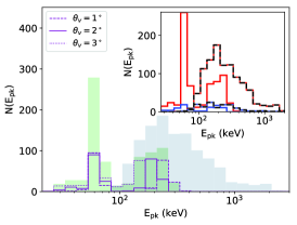
Figure 5.— Distributions of the fitted Band and COMP Parameters for the total simulation set. The grey histograms are the fitted parameters from Yu, Hoi-Fung et al. (2016). The distributions are separated by viewing angle and are shown by the purple dashed, solid, and dotted lines for $\theta_{\text{v}}=1^{\circ},2^{\circ}$ and $3^{\circ}$, respectively. The inset plots show the distributions of the simulation set and the FERMI data set differentiated by whether the COMP or Band function was used to acquire the parameter, with the exception of the $\beta$ distribution since that is only defined for the Band function. The COMP is shown in red, the Band parameters are shown in blue, and the FERMI data is shown as a red and black dotted line or a blue and black dotted line, corresponding to a COMP or Band fit, respectively.

The best fit parameters are collectively shown in Figure 5, for the 16OI, 16TI, 35OB, 16TI.e150.g100, and 16TI.e150 progenitors. The parameters for the full simulation set are grouped together and compared to the FERMI data, shown in grey. The different distributions for each viewing angle are shown by the purple dashed, solid, and dotted lines for $\theta_{\text{v}}=1^{\circ},2^{\circ}$ and $3^{\circ}$, respectively. The inset plots, for $\alpha$ and $E_{pk}$, show how the distribution of fitted parameters change between the COMP fits, in solid red, and the Band fits, in solid blue. The FERMI data is also split into COMP and Band fits which are represented by red and blue dotted lines, respectively.

Looking at the distribution of fitted $\alpha$ parameters, irregardless of the type of function that was used in the fit, it is easy to see that our low energy spectral indices average around $\sim 0.5$ while the FERMI distribution is clustered around $\sim-0.75$. On the other hand, our distribution of $E_{pk}$ coincide relatively well with FERMI’s distribution of the peak energy for all simulations except for the 16TI.e150.g100 and 16TI.e150 simulations. These simulations make up the large number of spectra with energies less than $\sim 100$ keV. This is to be expected since those simulations have lower engine luminosity. Overall, the majority of our spectra are well fit by the COMP spectrum which is to be expected since we are solely considering Compton scattering. However, we do have spectra where the Band function provides a statistically superior fit. Analyzing our Band $\beta$ parameters and comparing them to the FERMI distribution, we show that the observed Band $\beta$ parameter can be reproduced in a significant number of cases. This is due solely to photons being upscattered near the photosphere, which is a consequence of the fuzzy photosphere or “photospheric region” (Pe’er, 2008; Beloborodov, 2010).

The preference for a COMP fit over a Band spectrum is not a unique feature of our synthetic spectra. As a matter of fact, observed time-resolved spectra also display a preference for a COMP fit with 69.1% of the spectra being fit with the COMP model (Yu, Hoi-Fung et al. 2016). As Yu, Hoi-Fung et al. explain, the preference to the COMP model is due to low photon counts at high energies, reducing the ability for a model to fit those high energy bins well. Since our simulations emulate a typical GRB observation by binning photons in time, space, and energy, our simulations suffer from these low statistics as well. Figure 6 shows spectral points that were not included in the original fit of the 16TI time resolved spectrum, at $t=20-21$s, due to low photon counts; if such rejected points are included in the curve fitting, the preferred fit becomes the Band function instead of the COMP function. In order to compensate for low photon counts we will need to inject more photons in our simulations in the future; of course, this will be at the expense of computational time.

It is enticing that only considering Compton scattering our synthetic spectra can reproduce nearly all the observational features of GRB prompt spectra, with the notable exception of the low energy index $\alpha$. We show the time-integrated spectra for various simulations and viewing angles in Figure 4. The parameters for the best fit spectrum are shown on each plot. Figure 4(a) is best fit with a Band function although each time resolved spectrum is best fit with the COMP spectrum, showing that various thermalized spectra can add together to form a non-thermal spectrum. On the other hand, the time-integrated spectrum of the 35OB simulation at $\theta_{\text{v}}=1^{\circ}$, in which every time resolved spectrum is best fit with the COMP spectrum, is also best fit by the COMP function, as shown in figure 4(b). The time-integrated spectrum of the 16TI.e150.g100 simulation at $\theta_{\text{v}}=3^{\circ}$, which is best fit with the Band function, as shown in figure 4(c), is formed from time resolved spectra which are best fit by both the Band and COMP functions.

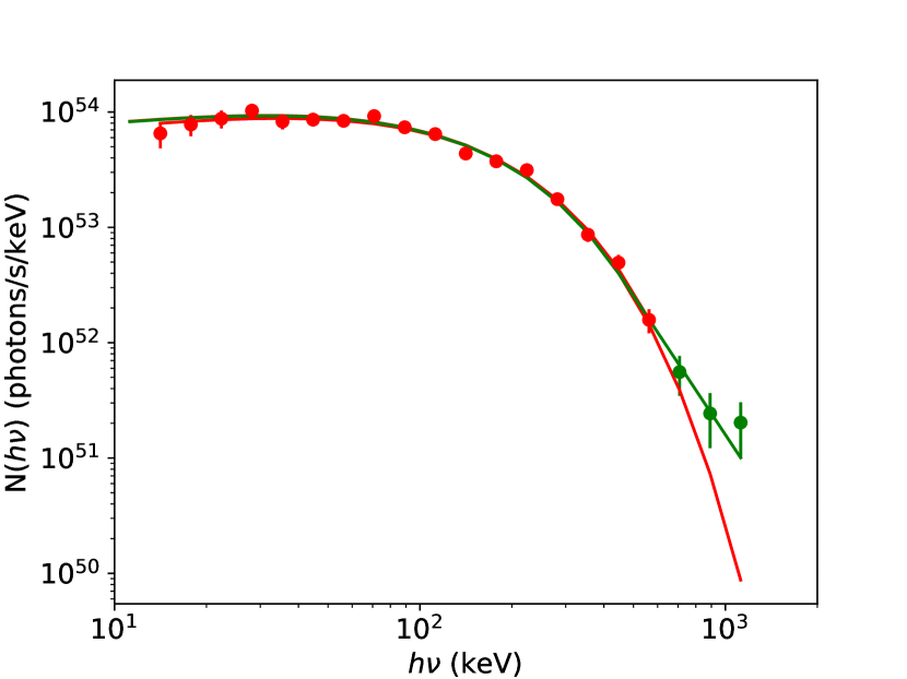
Figure 6.— The points with $>$10 photons in their respective bins are shown in red with the COMP best fit plotted in red. The green points are bins that were excluded from the analysis due to low photon counts, however, if these bins are included in the fitting then the best fit function becomes the Band function, plotted as the green line.

Another important aspect of our results is that the calculation of $E_{pk}$ is dependent on the fits for $\alpha$, which is greater than what is observed by $\sim 1$. This causes our peak energies to be somewhat artificially high. The issue of correctly reproducing the $\alpha$ parameter is a well known issue in the photospheric model. It can be fixed by including photon emitting processes, such as a synchrotron component. As the spectrum becomes corrected, with a larger number of low energy photons producing the proper values of $\alpha$, we would expect $E_{pk}$ to decrease (Beloborodov, 2013).

3.4. Comparison to Observational Relations

The time-integrated light curve and spectra from our simulations provide the necessary data for a comparison with GRB ensemble distributions, such as the Amati and Yonetoku correlations (Amati, L. et al., 2002; Yonetoku et al., 2004). The simulated data is plotted in the Yonetoku phase space alongside data from Nava et al. (2012) in Figure 7; the gray circles are the observed LGRB data, the blue line is the fit to the data, the star, diamond, and triangle markers represent our synthetic data points at $\theta_{\text{v}}=1^{\circ},2^{\circ}$ and $3^{\circ}$, respectively. Each MCRaT simulation is uniquely identified by a different color. It is clear that all the simulation points lie slightly below the fitted line. However, the simulation points are well within the spread of the data and the slope of the correlation is reproduced.

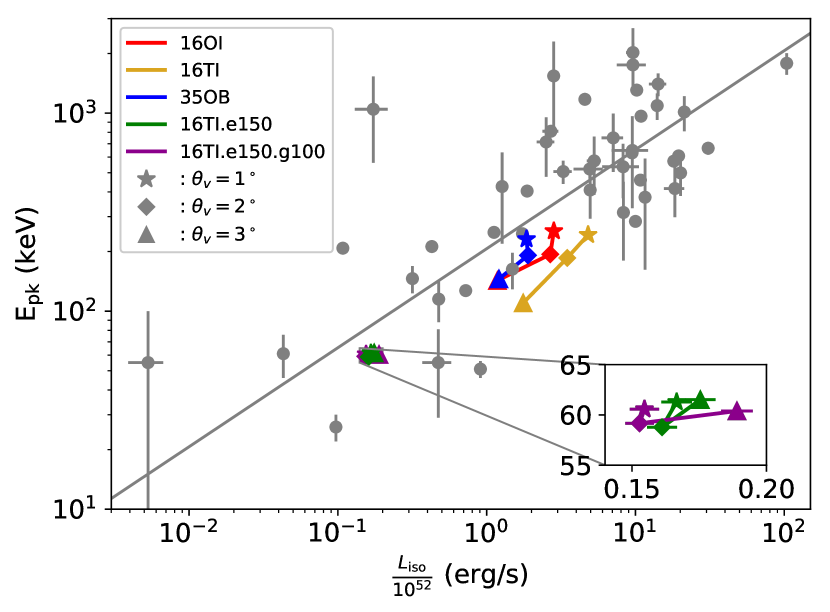
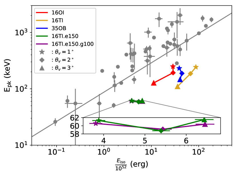
Figure 7.— The Yonetoku Relation (in the left plot) and the Amati relation (in the right plot). The isotropic luminosities and isotropic energies are normalized by $10^{52}$. The observational data and the fitted relations are plotted in grey as a circle marker or a line respectively. The simulation data points are shown in color and each viewing angle is differentiated by various marker types.

The same simulation results are plotted alongside the Amati relationship in Figure 7 using the same data set by Nava et al. (2012). In this case, the strain with the observations is more evident, possibly due to en excessive activity time of the engine in the FLASH simulations (the engine was active for 100 s, while observations point to a shorter activity time of $\sim 20$ seconds (Lazzati et al., 2013b; Hamidani et al., 2017).

4. Summary and Discussion

We have used the Monte Carlo Radiation Transfer code (MCRaT, Lazzati (2016)) to test the photospheric model for a variety of long Gamma Ray Burst (LGRB) simulations. MCRaT only considers Compton scattering, as photons are injected and propagated through the LGRB jet, and does not have the capabilities to investigate non-thermal particles or synchrotron radiation – at this time. Even though we neglect these important mechanisms that affect radiation, we are still able to reproduce a variety of LGRB characteristics and investigate their underlying causes.

We show that the matter and radiation counterparts of the LGRB jet gradually decouple from one another. This allows the photons to continually interact with the much cooler jet material, thus permitting the average photon energy to decrease even further. Photons encounter the photosphere, and are no longer interacting with the jet, when the average temperature of the photons become constant. In this work we also show that the photosphere for a given LGRB moves within a region of space, which we call the “photospheric region”. The dynamic nature of the photosphere is due to the variable density profile in the jet and can affect the spectra of the photons as the photons interact with the material in the jet for variable periods of time. The work done in this paper exhibits the importance of combining realistic jet dynamics with radiation transport calculations.

Some populations of photons within our simulation set never reach their respective photospheres and, as a result, are unable to fully cool to a steady state spectrum. This is due to the small domain of the FLASH simulation and can be easily remedied with larger domain simulations that allow the matter to cool for a longer period of time.

Additionally, we are able to reproduce the observational values of the Band $\beta$ parameter in our time resolved simulation spectra. This gives credence to the photospheric model, although the model still significantly suffers from a lack of low energy photons, which is exhibited in our extremely high values of $\alpha$. Our results show that acquiring Band $\alpha$ parameters that are close to the observationally expected $\sim-0.75$ is not possible with just Compton scattering. The peak energies, however, are consistently in the range of FERMI measurements, with the exception of the simulations which have lower jet luminosities (i.e. the 16TI.e150 and 16TI.e150.g100 simulations). This success is affected by the fact that our acquired values of $\alpha$ play a role in the calculation of $E_{pk}$. Since our values of $\alpha$ are too high, our values for the $E_{pk}$ become artificially high as well. Thus, the importance of correcting the Band $\alpha$ parameter increases. In order to correct this, we need to invoke a photon-producing radiation mechanism that will provide an extra supply of low energy photons. This is likely where synchrotron emission will come into play. The region in which these radiation mechanisms will play a large role is in the sub-photospheric region, where the radiation and the matter in the jet barely interact, allowing the low energy photons to escape from the jet after undergoing a minimal number of interactions without being thermalized. This would be possible since Lazzati et al. (2009) showed that shocks, which can reactivate magnetic fields, do extend all the way up to the photosphere.

By looking at the time-integrated simulation spectra of the 16OI simulation at $\theta_{\text{v}}=1^{\circ}$, we show that it is possible to produce a spectrum where the best fit is the Band function although each time resolved spectrum of the given simulation is best fit with the COMP function. This effect can be caused by the fact that many of the time resolved spectra were best fit with the COMP function due to the exclusion of spectral energy bins in which there were low photon counts. As the time resolved spectra are added up, the high energy spectral bins gain enough photons to be included in the fit of the spectrum, thus permitting the spectrum to be fit by the Band function in a statistically significant manner. This effect is not seen in our 35OB simulation at $\theta_{\text{v}}=1^{\circ}$, which means that some of the spectra may be intrinsically thermal. The time resolved spectral fits and light curves for the 16OI, 35OB, and 16TI.e150.g100 simulations are also presented. These light curves exhibit the photospheric model’s ability to recreate some of the observed relationships between the peak energy and the luminosity. We can recreate the observed hard-to-soft evolution of $E_{pk}$, and the tracking behavior between $E_{pk}$ and luminosity. We also see, in some cases, an anti-correlation between $E_{pk}$ and luminosity which is not commonly observed.

The simulation set used in this paper are all shown to lie marginally below the Yonetoku relation, but well within the spread of the data, which is encouraging. The same simulations are in tension with the Amati relation. The discrepancy with the observational relations further show the importance of including a sub-dominant radiation mechanism in order to correct the spectra. This would correct the Band $\alpha$ parameter but also push the peak energy of the spectrum towards lower energies, as Beloborodov (2013) points out. In order to correct the low spectral energies, we will need to consider sub-photopsheric shocks such as those considered by Beloborodov (2017). These shocks are capable of producing high energy non-thermal particles that will scatter off of photons and increase the average photon energy. With the production of low energy and high energy photons, it then becomes important to include absorption, which can be facilitated through pair production. Emission and absorption processes will be included in future versions of MCRaT, in order to self consistently treat the radiation transfer problem.

As with all hydrodynamic simulations, there is a concern with resolution being sufficient to resolve small scale features such as jet re-collimation shocks, which can create non-thermal particles. This concern is especially serious at large radii, where the spectrum forms. There is also concern with the number of photons that we inject into the simulation. The binning of photons in time, space and energy can quickly whittle down the number of photons available for spectral analysis thus affecting our spectral fits and our comparisons with theory. In order to circumvent this problem, we simply need to inject more photons into the MCRaT simulation, which will increase the computation time for a given simulation.

References

- Amati, L. et al. (2002) Amati, L., Frontera, F., Tavani, M., et al. 2002, A&A, 390, 81
- Band et al. (1993) Band, D., Matteson, J., Ford, L., et al. 1993, The Astrophysical Journal, 413, 281
- Beloborodov (2010) Beloborodov, A. M. 2010, Monthly Notices of the Royal Astronomical Society, 407, 1033
- Beloborodov (2013) —. 2013, The Astrophysical Journal, 764, 157
- Beloborodov (2017) —. 2017, The Astrophysical Journal, 838, 125
- Chhotray & Lazzati (2015) Chhotray, A., & Lazzati, D. 2015, The Astrophysical Journal, 802, 132
- Goldstein et al. (2013) Goldstein, A., Preece, R. D., Mallozzi, R. S., et al. 2013, The Astrophysical Journal Supplement Series, 208, 21
- Golenetskii et al. (1983) Golenetskii, S. V., Mazets, E. P., Aptekar, R. L., & Ilyinskii, V. N. 1983, Nature, 306, 451
- Hamidani et al. (2017) Hamidani, H., Takahashi, K., Umeda, H., & Okita, S. 2017, Monthly Notices of the Royal Astronomical Society, 469, 2361
- Ito et al. (2015) Ito, H., Matsumoto, J., Nagataki, S., Warren, D. C., & Barkov, M. V. 2015, The Astrophysical Journal Letters, 814, L29
- Ito et al. (2014) Ito, H., Nagataki, S., Matsumoto, J., et al. 2014, The Astrophysical Journal, 789, 159
- Ito et al. (2013) Ito, H., Nagataki, S., Ono, M., et al. 2013, The Astrophysical Journal, 777, 62
- Kulkarni et al. (1999) Kulkarni, S. R., Djorgovski, S. G., Odewahn, S. C., et al. 1999, Nature, 398, 389
- Lazzati (2016) Lazzati, D. 2016, The Astrophysical Journal, 829, 76
- Lazzati et al. (2009) Lazzati, D., Morsony, B. J., & Begelman, M. C. 2009, The Astrophysical Journal Letters, 700, L47
- Lazzati et al. (2013a) Lazzati, D., Morsony, B. J., Margutti, R., & Begelman, M. C. 2013a, The Astrophysical Journal, 765, 103
- Lazzati et al. (2013b) Lazzati, D., Villeneuve, M., López-Cámara, D., Morsony, B. J., & Perna, R. 2013b, Monthly Notices of the Royal Astronomical Society, 436, 1867
- López-Cámara et al. (2014) López-Cámara, D., Morsony, B. J., & Lazzati, D. 2014, Monthly Notices of the Royal Astronomical Society, 442, 2202
- Lundman et al. (2013) Lundman, C., Pe’er, A., & Ryde, F. 2013, Monthly Notices of the Royal Astronomical Society, 428, 2430
- Lundman et al. (2014) —. 2014, Monthly Notices of the Royal Astronomical Society, 440, 3292
- Nava et al. (2012) Nava, L., Salvaterra, R., Ghirlanda, G., et al. 2012, Monthly Notices of the Royal Astronomical Society, 421, 1256
- Pe’er (2008) Pe’er, A. 2008, The Astrophysical Journal, 682, 463
- Preece et al. (2002) Preece, R. D., Briggs, M. S., Giblin, T. W., et al. 2002, The Astrophysical Journal, 581, 1248
- Rees & Meszaros (1994) Rees, M. J., & Meszaros, P. 1994, ApJ, 430, L93
- Rees & Mészáros (2005) Rees, M. J., & Mészáros, P. 2005, The Astrophysical Journal, 628, 847
- Rybicki & Lightman (1979) Rybicki, G. B., & Lightman, A. P. 1979, Radiative processes in astrophysics
- Vurm & Beloborodov (2016) Vurm, I., & Beloborodov, A. M. 2016, The Astrophysical Journal, 831, 175
- Woosley & Heger (2006) Woosley, S. E., & Heger, A. 2006, The Astrophysical Journal, 637, 914
- Yonetoku et al. (2004) Yonetoku, D., Murakami, T., Nakamura, T., et al. 2004, The Astrophysical Journal, 609, 935
- Yu, Hoi-Fung et al. (2016) Yu, Hoi-Fung, Preece, Robert D., Greiner, Jochen, et al. 2016, A&A, 588, A135