Using Graph Properties to Speed-up GPU-based Graph Traversal: A Model-driven Approach

Abstract

While it is well-known and acknowledged that the performance of graph algorithms is heavily dependent on the input data, there has been surprisingly little research to quantify and predict the impact the graph structure has on performance. Parallel graph algorithms, running on many-core systems such as GPUs, are no exception: most research has focused on how to efficiently implement and tune different graph operations on a specific GPU. However, the performance impact of the input graph has only been taken into account indirectly as a result of the graphs used to benchmark the system.

In this work, we present a case study investigating how to use the properties of the input graph to improve the performance of the breadth-first search (BFS) graph traversal. To do so, we first study the performance variation of 15 different BFS implementations across 248 graphs. Using this performance data, we show that significant speed-up can be achieved by combining the best implementation for each level of the traversal. To make use of this data-dependent optimization, we must correctly predict the relative performance of algorithms per graph level, and enable dynamic switching to the optimal algorithm for each level at runtime.

We use the collected performance data to train a binary decision tree, to enable high-accuracy predictions and fast switching. We demonstrate empirically that our decision tree is both fast enough to allow dynamic switching between implementations, without noticeable overhead, and accurate enough in its prediction to enable significant BFS speedup. We conclude that our model-driven approach (1) enables BFS to outperform state of the art GPU algorithms, and (2) can be adapted for other BFS variants, other algorithms, or more specific datasets.

1 Introduction

Graph processing is an important part of data science, due to the flexibility of graphs as models for highly interrelated data. Given the rapid growth of dataset sizes, as well as the expected complexity increase of graph processing applications, a lot of research focuses on parallel and distributed solutions for graph processing [1, 2, 3, 4, 5, 6, 7, 8, 9, 10, 11].

With the increased popularity of graphics processing units (GPUs), some of this research also “migrated” to these massively parallel architectures. Tempted by the high-performance potential of GPUs, researchers investigate novel ways to circumvent the (apparent) lack of regularity and data locality [12] in graph processing to accommodate the massive parallelism of GPUs. Therefore, several GPU-enabled graph processing frameworks have emerged [3, 13, 14, 15, 16, 17].

Most graph processing frameworks, GPU-enabled or otherwise, simplify working with graphs by hiding complexity; they maintain a separation between a front-end that lets users specify their algorithm using high-level primitives or domain specific languages, and a back-end that provides high-performance implementations of these primitives for the given software or hardware platform.

Unfortunately, there is no consensus which primitives form the “canonical set“ of operations required to implement graph algorithms. It is not even clear if such a set exists. As a result, different frameworks choose drastically different primitives to base their implementation on, e.g., Gather-Apply-Scatter [18, 19] or vertex-centric operations [20, 1, 21]. To make matters worse, there are often many different ways to implement the same primitive, e.g., push versus pull for vertex-centric primitive [10].

If the performance of these primitives and implementations was only dependent on the hardware, this would be a tractable optimisation problem: benchmark each implementation for each piece of hardware and you can select a single “best“ performing implementation for your system. This is an arduous task, but not especially complicated.

But the performance of different implementations also depends on the structural properties of the graph being processed. While it is accepted as common knowledge that the performance of data-dependent algorithms is impacted by the structure of the data, little progress has been made, for graph processing, in understanding how large this impact is, or in modeling the correlation between the properties of the input data and the observed performance [22, 23, 24].

Theoretically speaking, there are multiple solutions to understand and/or quantify this correlation: (1) workload characterization and analytical modeling, (2) controlled (micro)benchmarking, or (3) statistical modeling.

While workload characterization for graph processing on parallel systems has been attempted, there is no such work to be found for GPUs. Moreover, there is very little work in analytical modeling for parallel graph processing, precisely because the strong dependence between hardware, algorithm, and dataset.

In our previous work we attempted to determine the performance impact of different graph properties by constructing an analytical model of the sequential workload of the implementation. We attempted to link graph properties to runtime behaviour [23], via metrics like: 1) access coalescing, 2) occupancy, 3) branch divergence, 4) atomic retries. Although the model was able to correctly estimate the amount of work per (algorithm, dataset) pair, its generalization for parallel execution on GPUs was less successful. Therefore, the resulting model had to be discarded due to its low average accuracy.

Controlled (micro)benchmarking is another interesting approach, where by a clever selection of the input datasets, we can study the changes in algorithmic performance behavior and eventually isolate the performance impact of each graph feature. In order for this approach to work, a large collection of (synthetic) datasets is required, in which each property can be varied in isolation.

No repository of such datasets exists. Instead, most research on graph processing uses: 1) input data from several publicly available real world datasets, such as SNAP [25] and KONECT [26], or 2) synthetically generated graphs using well-known generators/models, such as R-MAT [27], Kronecker graphs [28], and scale-free graphs [29].

The real world datasets are too noisy for systematic benchmarking; the graphs vary in almost every property. The synthetic graphs, although more predictable and controllable, still do not cover all properties of interest, and results cannot be generalised to other types of graphs. We attempted to generate graphs with the desired properties ourselves, but were unable to scale the generation to graphs of sufficient size to do benchmarking [30].

In this work, we focus on the third option towards understanding the performance impact of dataset properties on graph processing: data-driven. Specifically, we collect a lot of performance data from representative graphs, and we use it as training data for a machine learning approach towards a model that can predict performance for a given, unseen graph. While this approach provides less insight into the actual correlations, it does provide a systematic process for building a prediction model, and many tuning possibilities in terms of features, variables, and actual methods.

Among all these methods, we initially selected Random Forests as the predictive model, and found its accuracy to be good, but its applicability for fast prediction too limiting. To simplify the model, we opted for a Binary Decision Tree (BDT), and found it provides a good balance between accuracy and applicability. Therefore, this work focuses on building and using a BDT-based model to: 1) determine which graph properties have the biggest impact on algorithm performance, and 2) improve the BFS performance by predicting and deploying the best performing algorithm for each BFS level.

We have applied this model on the 248 graphs from KONECT; for each graph we used 20 different traversals, starting from 20 different nodes, and collected the features and performance indicators for each traversed level. We trained the model on a 70% random split of the data. When testing on the remaining 30% of the data, the model predicts with 96% accuracy. Finally, we use the model as a switch predictor for a level-switching adaptive BFS. With this adaptive BFS, we outperform two popular graph processing systems for GPUs: we gain on average $2{\times}$ over Gunrock [13] and $15{\times}$ over LonestarGPU [31].

The main contributions of this paper are the following:

• We show that the performance of different BFS implementations varies dramatically across both graphs and iterations within the same graph, with differences of up to two orders of magnitude (Section 3).

• We create a binary decision tree model that can predict which BFS implementation to use at every level of BFS. (Section 4.1).

• We show that our decision-tree model is accurate enough and fast enough to evaluate online, allowing for dynamic switching of implementations during BFS (Section 4.3).

• We demonstrate that using our dynamic switching BFS approach, enabled by the accurate prediction of our model, may lead to performance gains of ${\sim}20\%$ to ${\sim}80\%$ over the best single-algorithm BFS (Section 4.3).

2 Background

For readers unfamiliar with binary decision trees or GPGPU processing, this section provides some basic information required to understand the rest of this paper.

2.1 Decision Trees

Decision trees are a non-parametric, supervised learning technique [32]. They come in two flavours, classifiers and regressors. After constructing a decision tree from a training set of $(X,Y)$ pairs, where $X$ is a tuple of 1 or more inputs and $Y$ is a tuple of 1 or more outputs, we can use this tree to predict the expected output tuple for a given input tuple. The working assumption is that the original learning set is representative of the observable input-output pairs.

To construct a (binary) decision tree we recursively partition the learning set along one of the $N$ input parameters, preferring the parameter (and value) that has the strongest discriminating power, i.e. the one that produces the partitioning closest to 50–50. The split effectively means that we assign all elements smaller than the chosen value to the left branch and the others to the right branch. This process repeats until we reach a stopping criteria — e.g., the maximum tree height, minimal bucket size.

After the stop condition is hit, the output for each bucket is computed. If the bucket contains 1 output value, or multiple equal outputs, this is the result for that bucket. If there are multiple unequal values, the outputs are normalised to a single output. For regressions this usually done by averaging all values in the bucket. For classification, this is usually by selecting the “most likely” value in the bucket, although more complicated strategies exist.

We can now use this computed binary tree as a prediction model. To compute a prediction using this tree for an input tuple, we compare the tuple’s value against the parameter stored in the tree at each level, and walk down the correct branch. Once we reach a leaf node, we return the value computed above for that bucket as resulting prediction.

Different decision tree algorithms use different criteria to compute which parameter and value to split the tree on. We used the implementation in Python library scikit-learn [33]. This uses an optimised algorithm based on the CART [32] algorithm. This algorithm splits the training set based on which parameter produces the large reduction in Gini impurity. Gini impurity is a measure of how often an element in a subset would labelled wrong if all elements in the subset were labelled randomly, according to the distribution of labels in that subset.

We can estimate the importance of each input parameter by computing its Gini importance. This is done by computing the total, normalised, reduction of Gini impurity resulting from that parameter. Similar importance measures exist for other decision tree algorithms, meaning that we can relatively easily compute the importance of each parameter in our input.

To summarise the advantages of decision trees: They are simple to understand and interpret; Small trees can be visualised; They require little to no data preparation; Prediction cost is logarithmic in the number of data points used; They can handle both categorical and numerical data; They can handle multi-output problems; Parameter importance is known after training.

The main downsides of decision trees are: They are prone to overfitting; Small differences in data can result in drastically different results (i.e., unstable models); Constructing optimal decision trees is NP-complete under several aspects of optimality; They cannot represent all concepts easily (XOR, parity, multiplexer problems); Biased trees are easily created, if some classes dominate.

Due to the way trees are constructed, overfitting issues can become more pronounced if the input parameters in the learning set are not uniformly distributed across the range we intend to predict against. Additionally, as the number of input parameters increases it becomes exponentially more costly to compute the best discriminator, which in turn makes the algorithm slower and increases the risk of bias and overfitting. To reduce and detect overfitting we train our decision trees on a random subset of our data points and cross-validate our model against the unseen data points. See Section 4.4 for a more detailed discussion on concerns related to overfitting.

2.2 Graph Processing

Graphs are collections of entities (called nodes or vertices) and relationships between them (called edges) — $G=(V,E)$. Graph processing typically implies some transformation of the original graph by traversing its edges and visiting is nodes. The simplest example itself being a traversal itself, where, given a starting node (also called the root node), the algorithm has to visit all the nodes accessible from the root, eventually providing shortest path between the root and all accessible nodes. There are two types of traversals: the Breadth-First Search (BFS) and Depth-First Search (DFS). In this work we focus mainly on BFS.

In general, graph processing applications — and traversal is a good example — are not easy to parallelize due to their properties: low compute-to-communication ratio, data-dependent behavior, low data locality, variable parallelism, and load imbalance, etc. Thus proposing efficient parallel algorithms for these algorithms is a challenge.

2.3 General Purpose GPU Programming

GPUs (Graphics Processing Units) are the predominant accelerators for high performance computing. A GPU is, currently, a very good example of a many-core architecture: it has hundreds to thousands of slim cores, grouped into streaming multi-processors with local shared memory and/or caches; it provides a hierarchical memory model, with large register files per multi-processor, local L1 and shared L2 caches, and a global memory which increases in size with every generation.

GPUs promise huge theoretical performance: the peak performance of a regular card can easily be in excess of 2 TFLOPs computational throughput and 200–300 GiB/s memory bandwidth. With such performance numbers, sooner or later, all computational domains will investigate whether GPUs are a suitable target for their computational needs.

Graph processing is no exception: our work focuses on understanding the potential for GPUs to boost the performance of graph processing algorithms, which are notoriously difficult to parallelize efficiently. In this work, we use NVIDIA GPUs, due to their superior programmability provided by CUDA.

The idea behind the programming model is simple: CUDA provides a mapping of the programming model concepts onto the hardware, while preserving a sequential programming model per thread. For the actual computation, programmers focus on implementing the single-thread code, called a kernel; they further write the host code to launch enough threads to (1) cover the space of the problem, and (2) provide enough potential for latency hiding [34, 35]. The threads that execute the kernel are grouped into thread blocks, which are scheduled on the streaming multi-processors. All blocks form a grid, which effectively contains all the logical threads that are to be scheduled and eventually executed on the cores themselves.

In terms of the execution model, NVIDIA GPUs work with warps. A warp is a group of 32 threads that work in lock-step: they all execute the same instruction on multiple data. This model is called SIMT — Single Instruction Multiple Thread — and enables high performance by massive parallelism, but is unable to handle diverging threads, it also poses programming challenges to avoid the severe penalties that any inner-warp load imbalance might bring. Besides thread divergence, other performance challenges in GPU programming are the abuse of atomic operations and lack of coalescing for the main memory accesses.

Our software stack is based on C++ and CUDA, and it is available on GitHub.

3 Experiments

We benchmarked our 15 different BFS implementations on the graphs found in the KONECT [26] dataset, measuring both the total time and the time taken for each level of BFS. We used these results to train and validate our Binary Decision Tree (BDT) model.

3.1 BFS Implementations

We wrote 5 different implementations of BFS, and for each of these 5 implemented 3 variants. These 5 implementations consist of: 2 edge-centric implementations (edge list and reverse edge list), 2 vertex-centric implementations (vertex push and vertex pull), and 1 virtual warp-based implementation based on the work by S. Hong and Olukotun [36]. The 3 different variants are based on how the new frontier size is computed at the end of each BFS level. In this subsection we describe how these versions differ from each other.

Each algorithm starts by initialising all depths to infinity, then initialising the root node’s depth to 0. During every level of BFS we compute the frontier size, that is, the number of vertices that have been assigned a new depth.

3.1.1 Edge List & Reverse Edge List

For every level of BFS these edge-centric implementations launch one CUDA thread per edge. If the depth of the origin vertex is equal to the current BFS level, then the depth of the destination vertex is updated to the minimum of its current depth and the BFS level plus one.

The edge list implementation uses the outgoing edges of every vertex, whereas the reverse edge list implementation use the incoming edges of every vertex. This difference affects the amount of memory coalescing and the access patterns exhibited at runtime.

The advantage of these edge-centric parallelisations is that they never suffer from workload imbalance, every thread in a warp performs the same amount of work. The fact that many threads have to read the depth of the same origin vertex helps with coalescing memory access. The downside is that they result in many parallel updates, resulting in many heavily contested atomic updates.

3.1.2 Vertex Push & Vertex Pull

For every level of BFS these vertex-centric implementations launch one CUDA thread per vertex. For the push implementation, if the vertex its depth is equal to the current BFS level, the thread iterates over all its neighbours, updating their depth to the minimum of their current depths and the BFS level plus one. For the pull implementation, if the vertex has no depth yet, the thread iterates over its neighbours until it encounters one whose depth matches the current BFS level, if this happens it sets its depth to the current BFS level plus one.

Both implementations are susceptible to workload imbalance, if vertices with wildly different degrees are in the same warp, this divergence will result in reduced performance. The push version, similar to edge-centric implementations generates a lot of concurrent updates, requiring a large number of atomic operations. However, if the frontier is small it avoids many useless reads, since the depth of every vertex is only read once.

The pull version does not require atomics as the depth of a vertex is only ever touched by one thread. The downside is that, if none of a vertex its neighbours are in the frontier, a lot of time is wasted iterating over neighbours for nothing. As such pull becomes more efficient as more vertices are in the frontier, since a thread can stop looping over its neighbours as soon as it discovers one in the frontier.

3.1.3 Vertex Push Warp

As mentioned above, this implementation is based on the vertex push implementation, but rather than assigning one thread per vertex, it uses the virtual warp method described in [36], which attempts to mitigate the negative impact produced by workload imbalance between threads.

The basic principle is the same as with vertex push, but rather than assigning a single thread per vertex, we divide the warps into smaller “virtual warps”. Each virtual warp gets assigned a number of vertices, equal to its number of threads. However, instead of each thread processing the edges for one vertex, all $N$ threads process the edges of the first vertex in parallel, then the edges of the second vertex are processed in parallel, and so on until all vertices assigned to the virtual warp have been processed.

This reduces the amount of load imbalance occurring within a virtual warp, since the workload of a virtual warp is spread out equally across that virtual warp. However, the optimal size of the virtual warp is challenging to determine. Moreover, the different graphs and even different levels of the graph also require tuning of the warp sizes for best performance.

3.1.4 Variants

In every BFS level, 0 or more new vertices get discovered. These vertices will form the frontier for the next level. We need to track the size of the frontier, since the algorithm terminates when no new nodes are discovered. To accomplish this task, each thread tracks how many new vertices it has discovered. At the end of each BFS level, we need to aggregate these counts to compute the new frontier size.

We implemented three different methods to do this aggregation. The first variant simply uses a global counter and every thread performs an atomic addition on this counter. This approach results in heavily contested atomics operations. Most of the CUDA literature suggests that we can reduce the contention and number of atomic operations by first performing a reduction within a warp or block [37], before performing the global atomic operation. Thus, the second variant performs a warp reduction before the global atomic update, while the third variant performs a warp-and-block reduction before atomically updating the frontier size.

3.2 Experimental Setup

All measurements have been performed on an NVIDIA TitanX, using version 7.5 of the CUDA toolkit. The source code of these benchmarks can be found on GitHub.

As for datasets, we retrieved all the graphs from the KONECT repository and ran each of the $3\times 5$ implementations described above on all of them. Additionally, for every graph, we used 20 different root vertices. All results presented here are averaged over 30 runs, and exclude input data and result transfer times.

The first observation we made about our results is that both the warp reduction and warp-and-block reduction variants perform significantly worse than the direct atomic versions, in all cases. Therefore, we do not include any of these variants in the plots of this paper, to keep the results easily readable.

Figure 1 shows the runtimes, normalised to the slowest implementation for each graph, for a selection of KONECT graphs.

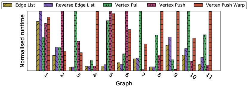
Figure 1: Normalised total runtimes for different BFS implementations on KONECT graphs. See Table I for the details of the input graphs.

No.	Graph	# Vertices	# Edges
1	actor-collaboration	382,219	30,076,166
2	ca-cit-HepPh	28,093	6,296,894
3	cfinder-google	15,763	171,206
4	dbpedia-starring	157,183	562,792
5	discogs_affiliation	2,025,594	10,604,552
6	opsahl-ucsocial	1,899	20,296
7	prosper-loans	89,269	3,330,225
8	web-NotreDame	325,729	1,497,134
9	wikipedia_link_en	12,150,976	378,142,420
10	wikipedia_link_fr	3,023,165	102,382,410
11	zhishi-hudong-internallink	1,984,484	14,869,484

TABLE I: Details for the input graphs shown in Figure 1 and Figure 3.

The plots in fig. 1 were selected to illustrate the point we made in the introduction: the performance of different implementations can vary by orders of magnitude across input graphs.This effectively means that when (accidentally) choosing the worst algorithm, one can loose 1–2 orders of magnitude in performance for a BFS traversal compared with the best option. In turn, this means an informed decision about the algorithm to be used for a given graph is not only desirable, but quite important for any efficiency metric. But this is no easy task: no models are available to determine the best or the worst algorithm for a given graph traversal task.

One of the reasons for which predicting the best algorithm for the entire graph is difficult is the huge performance difference that can be observed during traversing a single graph: (1) between two different BFS levels in the same graph, the performance of the same algorithm can vary up to an order of magnitude, and (2) per-level, the differences between different algorithms can be up to four orders of magnitude.

In over 75% of the cases the difference between the best and worst implementation for a single level is more than 2 orders of magnitude, and 4 orders of magnitude in the worst cases. This, combined with the fact that each algorithm wins at least once and loses several times, makes a random choice far from ideal for determining the implementation to use at a given level.

To illustrate these large performance gaps, fig. 2 presents an example of the performance of the five main BFS implementations, per-level, for the actor-collaborations graph. We see that the vertex push implementation dominates on most levels, but on a handful of levels it performs so badly that its overall performance becomes terrible. Such behaviour is a strong indication that switching algorithms at every level might be even better than devising a model to detect the best overall solution.

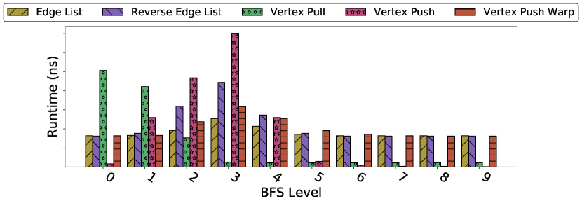
Figure 2: Runtimes of different BFS implementations per level of the actor-collaborations graph from KONECT.

4 Modeling BFS Performance

There is no consensus on which of a graph’s structural properties impact the performance of graph algorithms. Our previous modeling attempts in [23], combined with our experiences while optimising and developing our implementations lead us to believe that the graph size and degree distribution are the biggest factors when it comes to neighbour iteration. Additionally, the work of Beamer et al. and Li and Becchi on adaptive BFS [10, 16], and the observed runtime changes across levels, indicates that the behaviour at each level is dependent on the size of the frontier discovered in the previous level, and the percentage of the graph that has already been discovered. Therefore, these are the features we focus on when building a performance prediction model.

Further in this section we describe the training process used to build our model, discuss its accuracy and the applicability for online performance prediction, and analyse the feasibility of a dynamically switching BFS.

4.1 Building the model

The experiments described in the previous section provide us with timing data for all 15 of our algorithms and each BFS level of all KONECT graphs. This data allows us to compute the fastest implementation for each BFS level and graph combination. We built a training set where we associated every measured BFS level with the structural properties of the graph it was run on, and the level’s specific information. We consider the following relevant features for our model:

Graph size:

the number of vertices and edges in the graph.

Frontier size:

either as absolute number of vertices or as percentage of the graph’s vertices.

Discovered vertex count:

either as absolute number of vertices or as percentage of the graph’s vertices.

Degree distribution:

represented by the 5 number summary and standard deviation of in, out, or absolute degrees.

The models described in the rest of this section consist of binary decision trees trained to predict the best performing algorithm for a given level of BFS, based on a mix of the above properties. We remind the reader that the predicted value for each leaf in the tree is based on a majority vote on what is “most likely” given the values in the bucket associated with that leaf — see section 2.1). However, there can be special cases when the model cannot deliver a prediction because no single value can be computed based on the values in the bucket — e.g., as a result of a tie.

In such cases we talk about an “unknown prediction”. We opted to resolve unknown predictions for level $N$ of a BFS by repeating the prediction for level $N-1$. In case of an unknown prediction at the first level of BFS, we default to predicting the edge list implementation, as this implementation is the least likely to have extremely bad performance, which should reduce the likelihood of early unknown predictions resulting in significant performance loss.

4.2 Model Accuracy

We define the optimal BFS traversal of a graph as the traversal where the fastest of our implementations is used at every level. To evaluate the accuracy of our models, we take this optimal runtime as a reference (i.e., as 1) and evaluate the predicted and observed runtimes as a slowdown compared to this theoretical optimum. The larger the gap, the further away we are from the optimal performance.

Of the models we have trained using our experimental dataset, the one that performs best for this prediction task is one based on the following four features: graph size, percentage of vertices discovered, the distribution of out degrees, and the number of vertices in the current frontier. In table II we compare the model’s predictions and the different implementations against the optimal runtime across all KONECT graphs. The optimal runtime is the execution time of the optimal BFS traversal. The “oracle” runtime shows the fastest algorithm for every graph when dynamic runtime switching during the BFS computation is disabled (i.e., the best performing non-switching algorithm for each graph).

Algorithm	Optimal	1–2$\times$	${>}5{\times}$	${>}20{\times}$	Average	Worst
Predicted	$56\%$	$41\%$	$1\%$	$0.5\%$	$1.40{\times}$	$236{\times}$
Oracle	$23\%$	$55\%$	$2\%$	$0\%$	$1.65{\times}$	$8.5{\times}$
Edge List	$10\%$	$61\%$	$7\%$	$0.4\%$	$2.22{\times}$	$38{\times}$
Rev. Edge List	$5\%$	$59\%$	$15\%$	$0.6\%$	$2.92{\times}$	$50{\times}$
Vertex Pull	$0\%$	$15\%$	$27\%$	$24\%$	$38.62{\times}$	$2,671{\times}$
Vertex Push	$9\%$	$15\%$	$53\%$	$29\%$	$39.66{\times}$	$1,048{\times}$
Vertex Push Warp	$0\%$	$0\%$	$3\%$	$30\%$	$18.69{\times}$	$97{\times}$

TABLE II: Algorithm performance compared to theoretical optimum over all the graphs in KONECT.

Following our model’s predictions, we observe an average runtime of $1.40$ of optimal, which effectively means a 40% slowdown compared to optimal. However, the oracle average runtime is $1.65$, or 65% slowdown compared to optimal. In other words, by following the model’s prediction, we can obtain a 15% speedup compared to this oracle. In practice, the potential gain is more significant, as such an oracle does not exist.

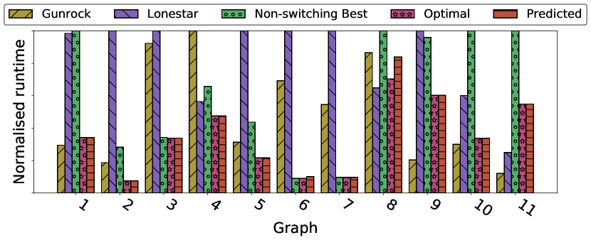
Figure 3: Comparison of normalised runtimes of different BFS implementations, predicted performance, and existing optimised BFS implementations on KONECT graphs. See Table I for the details of the input graphs.

These results show that our model results in considerable speedup compared to our individual implementations. However, speedup results are only as good as the baseline. We compare against two existing GPU graph processing frameworks to establish how much “real world” performance we gain by using the model described in this paper.

Figure 3 compares our results against the state-of-the-art GPU graph processing framework Gunrock [13] and the slightly older BFS benchmark LonestarGPU [31], across a selection of KONECT graphs. We benchmarked both Gunrock and LonestarGPU on the same hardware, using 148 different KONECT graphs. On average, Gunrock achieves a performance of $2.9{\times}$ of our theoretical optimum. LonestarGPU manages $21{\times}$ of optimal. Our model’s $1.4{\times}$ of optimal means that we are, on average, $2{\times}$ faster than Gunrock.

4.3 Feasibility of Dynamic Switching

The results presented in Section 3 indicate a significant performance improvement when switching between different implementations at runtime, but these gains can only be realised if the cost of switching does not outweigh the gains. Thus, the feasibility of dynamic switching effectively depends on (1) how long it takes to compute a prediction based on the trained model, and (2) how expensive a “context switch” is between these implementations.

To determine whether the runtime prediction is cheap enough, time-wise, we extracted the binary decision tree from scikit-learn, converted it into a C array-based data structure, and corresponding lookup function. We then measured the time it takes to compute a prediction for each graph and level in our dataset. The average prediction time is 144 ns, with a standard deviation of 161 ns, and a maximum of 16 $\mu$s. For comparison, the average BFS level computation in our dataset takes 28 ms. Thus, computing the prediction is, on average, insignificant compared with the actual processing of each level.

We still need to evaluate how expensive the “context switch” between implementations is. We note that most of our implementations operate on different representations of the graph, so to switch to a different implementation, we need to (a) either generate/bring the new representation in memory, or (b) simply keep all representations in memory.

Option (a) is not really feasible, because transferring data to and from the GPU is generally slow, and doing so for each level would become prohibitive, performance-wise. For option (b), we mush combine the two different representations into one, which is is a feasible solution, a classical time–space trade-off, where we trade memory for faster computation.

The two main graph representations we use are a Compressed Sparse Row (CSR) for the vertex-centric implementations, and an edge list for the edge-centric implementations. We can combine the two by simply storing the origin vertex for every edge in our CSR. This increases the storage from 1 int/vertex and 1 int/edge (for CSR) and 2 int/edge (for edge list), to 1 int/vertex and 2 int/edge. This is not very expensive, memory-wise: it is a mere 38 MiB for a graph of 10,000,000 edges.

4.4 Overfitting & Generality Concerns

As mentioned in section 2.1 we took the standard precaution of training our model against a subset of 70% of our data and validating its accuracy against a separate test set of 30% of the data points. In this validation, the model accurately predicts the fastest algorithm in 95% of the cases. The average difference in runtime between the fastest implementation and our predicted implementation is 9.9%.

From this data we can conclude that the model’s accuracy is high with regards to our KONECT repository of graphs. However, we expect the portability of the model to be highly correlated with how representative the training set is for the test set. For example, if we train the model on social networks graphs only, we expect it to be better at predicting the best BFS for social networks, and less so for, say, road networks. Therefore, we recommend that the actual training and modeling process is driven by the prediction goals.

For example, If the goal is to build a generic model to predict most graphs, using a large variety of graphs for training is mandatory. A collection like KONECT is a good start, but we have two indicators that it is not a balanced collection.

First, while validating the model against the KONECT data set, we noticed that bad model predictions are correlated with several classes of graphs, such as bipartite graphs, and graphs with extremely skewed degree distributions, which are less represented in the repository (and, thus, in our training data).

Second, we also used the model to predict algorithm selection for 19 graphs from the SNAP repository. For these graphs, our model performed significantly worse than for KONECT, achieving an average runtime of $3{\times}$ compared to optimal, or $2{\times}$ worse compared to an oracle that predicts the best non-switching algorithm. There are two plausible causes for these mis-predictions: (1) KONECT is indeed not representative enough of all graphs, causing our model to miss due to a lack of samples for specific cases, and (2) there are important structural properties not included in our current training data.

On the other hand, if the goal is to have a model tweaked for a specific type of graphs — e.g., social or road networks — only a subset of the graphs in public repositories can be useful for training. Whether there are sufficient such graphs depends on many factors. However, this analysis deserves a dedicated study, focused on determining what is the ideal size and composition of a specialized training set; such a study is beyond the scope of this work.

To summarize, we make no portability claims or guarantees of the trained model for more specialized repositories, and we recognize the limitations of our training dataset. However, the training and prediction processes are both straightforward and generic, and can be easily applied for different training, eventually improving/tuning the predictor to match the goal.

5 Related Work

This section briefly introduces relevant work from the three research directions closest to this work: (1) the design and implementation of parallel graph processing algorithms, (2) graph processing frameworks and systems for graph processing, and (3) the use of machine learning for performance modeling and prediction.

5.1 Algorithms

Despite the advances in large-scale graph traversal algorithms, like direction switching BFS [10], distributed-memory BFS [11], and the matrix-based graph processing solution [38], there’s still no single best BFS traversal solution. This is because BFS is highly dependent on the graph properties, with different algorithms and/or implementation eventually suffering from different bottlenecks.

When combining this with complex, massive parallel machines like the GPUs [17], the performance gaps are even more difficult to predict. In our work, we steer away from attempting to devise yet another algorithm for BFS, and focus on using the best existing solution in each iteration. A somewhat similar approach has been attempted in [16], but our solution combines more algorithms and uses a more deterministic, systematic switching criterion. Moreover, our approach can be extended to incorporate additional BFS versions, as long as sufficient performance data are available for training.

5.2 Graph Processing Systems

The new challenges of graph processing have also reflected in the amount of systems and frameworks designed for efficient, high performance graph processing [21, 39]. From these systems, a handful of GPU-enabled systems have also emerged [13, 31], combining clever BFS algorithms with specific GPU-based optimisations [36].

Still, none of them can claim the absolute best performance for the same reason: the diversity of graphs and their properties lead to high performance variability for all these systems [40]. This work is complementary to such systems: our switching approach can be, in principle, incorporated in these frameworks. Performance-wise, we are competitive against such systems (see Section 4.2), thus exploring the potential of incorporating such an adaptive approach into an existing system is promising as future work.

5.3 Machine Learning for Performance Modeling

Our adaptive BFS algorithm is based on performance prediction, which in turn is based on a machine learning model. Performance prediction based on machine learning has been attempted in many instances in the past [41, 42, 43, 44, 45, 46]. However, applying machine learning for an adaptive, level-switching BFS requires significant changes: features and variable selection, as well as the collection and selection of training data are specialized for the challenges of graph analytics. To the best of our knowledge, we are the first to have attempted training and using such a model for improving BFS performance by runtime switching.

In summary, our work is the first to employ a performance model based on machine learning for building a generalized version of the direction optimized BFS [10].

6 Conclusion

With the increased availability of large, complex graphs and the high demand for their analysis, high performance computing techniques become mandatory to handle large scale graph processing. Among these techniques, the use of massively parallel architectures like GPUs has been successful in the past: both new algorithms and new processing systems have been proposed to speed-up large scale graph processing.

Yet, despite the rapid innovation in the field, there has been little progress in quantifying the actual correlation between graph properties and the performance of graph analytics. In other words, the performance variability of graph processing, visible for most algorithms when processing different graphs and even when processing different layers of the same graph, has not been quantified and/or addressed.

In this work, we propose to use this variability to gain performance for a given graph processing algorithm: BFS traversal on GPUs. Our approach works as follows: given a set of BFS algorithms (15 in total), and an input dataset, we aim to determine and employ, for each level in the BFS traversal, the best algorithm in the available set. This is an generalization of the work on direction-switching BFS [10] and adaptive graph algorithms [16], to which we have added a much more systematic switching detection.

Specifically, we use machine learning concepts to train a prediction model, which is used at runtime to determine if switching is needed and, if so, to which variant we should switch. This combination of machine learning modeling and the large set of algorithms makes our approach competitive with state-of-the-art graph processing systems and algorithms.

Our findings are interesting in two different ways. First, we demonstrate high performance, with an average gain of $2{\times}$ over Gunrock and $15{\times}$ over LonestarGPU. Second, and more relevant for the original contribution of this work, we demonstrate that machine learning can be used to build a high-accuracy model which, taking into account graph and algorithm properties, can predict the optimal selection of BFS implementations for ${\sim}56\%$ of all BFS traversals and within $2{\times}$ of optimal for ${\sim}97\%$ of all traversals.

We conclude that this work is a step forward in quantifying and using the impact of graph properties on the performance of graph processing. For the near future, we plan to pursue three research objectives: design and automate an efficient training process, investigate the potential contribution of other BFS algorithms, and test other modeling techniques that offer a good balance between accuracy and speed of run-time evaluation. Finally, on the long term, we plan to use these results to actually understand the impact of graph properties on BFS graph traversal on GPUs.

References

- Avery [2011] C. Avery, “Giraph: Large-scale graph processing infrastructure on hadoop,” Proceedings of the Hadoop Summit. Santa Clara, 2011.
- Hong et al. [2015] S. Hong, S. Depner, T. Manhardt, J. Van Der Lugt, M. Verstraaten, and H. Chafi, “PGX.D: A fast distributed graph processing engine,” in Proceedings of the International Conference for High Performance Computing, Networking, Storage and Analysis. ACM, 2015, p. 58.
- Guo et al. [2015a] Y. Guo, A. L. Varbanescu, A. Iosup, and D. Epema, “An Empirical Performance Evaluation of GPU-Enabled Graph-Processing Systems,” in CCGrid’15, 2015.
- Lu et al. [2014] Y. Lu, J. Cheng, D. Yan, and H. Wu, “Large-Scale Distributed Graph Computing Systems: An Experimental Evaluation,” VLDB, 2014.
- Han et al. [2014] M. Han, K. Daudjee, K. Ammar, M. T. Ozsu, X. Wang, and T. Jin, “An Experimental Comparison of Pregel-Like Graph Processing Systems,” VLDB, 2014.
- Elser and Montresor [2013] B. Elser and A. Montresor, “An Evaluation Study of Bigdata Frameworks for Graph Processing,” in Big Data, 2013.
- Satish et al. [2014] N. Satish, N. Sundaram, M. A. Patwary, J. Seo, J. Park, M. A. Hassaan, S. Sengupta, Z. Yin, and P. Dubey, “Navigating the Maze of Graph Analytics Frameworks using Massive Graph Datasets,” in SIGMOD, 2014.
- Guo et al. [2014] Y. Guo, M. Biczak, A. L. Varbanescu, A. Iosup, C. Martella, and T. L. Willke, “How Well do Graph-Processing Platforms Perform? An Empirical Performance Evaluation and Analysis,” in IPDPS, 2014.
- Committee [2010] T. G. . S. Committee. (2010) The graph 500 list.
- Beamer et al. [2013] S. Beamer, K. Asanović, and D. Patterson, “Direction-optimizing breadth-first search,” Scientific Programming, vol. 21, no. 3-4, pp. 137–148, 2013.
- Buluç et al. [2016 (in press] A. Buluç, S. Beamer, K. Madduri, K. Asanović, and D. Patterson, “Distributed-memory breadth-first search on massive graphs,” in Parallel Graph Algorithms, D. Bader, Ed. CRC Press, Taylor-Francis, 2016 (in press). [Online]. Available: http://gauss.cs.ucsb.edu/~aydin/ChapterBFS2015.pdf
- A. Lumsdaine and Berry [2007] B. H. A. Lumsdaine, D. Gregor and J. W. Berry, “Challenges in parallel graph processing,” Parallel Processing Letters 17, 2007.
- Wang et al. [2016] Y. Wang, A. Davidson, Y. Pan, Y. Wu, A. Riffel, and J. D. Owens, “Gunrock: A high-performance graph processing library on the gpu,” in Proceedings of the 21st ACM SIGPLAN Symposium on Principles and Practice of Parallel Programming. ACM, 2016, p. 11.
- Heldens et al. [2016] S. Heldens, A. L. Varbanescu, and A. Iosup, “Dynamic load balancing for high-performance graph processing on hybrid cpu-gpu platforms,” in 2016 6th Workshop on Irregular Applications: Architecture and Algorithms (IA3), Nov 2016, pp. 62–65.
- Khorasani et al. [2014] F. Khorasani, K. Vora, R. Gupta, and L. N. Bhuyan, “CuSha: vertex-centric graph processing on GPUs,” in HPCS. ACM, 2014, pp. 239–252.
- Li and Becchi [2013] D. Li and M. Becchi, “Deploying graph algorithms on gpus: An adaptive solution,” in IPDPS 2013, May 2013, pp. 1013–1024.
- Buluç et al. [2010] A. Buluç, J. R. Gilbert, and C. Budak, “Solving path problems on the GPU,” Parallel Computing, vol. 36, no. 5-6, pp. 241 – 253, 2010. [Online]. Available: http://gauss.cs.ucsb.edu/publication/parco_apsp.pdf
- Gonzalez et al. [2012] J. E. Gonzalez, Y. Low, H. Gu, D. Bickson, and C. Guestrin, “Powergraph: Distributed graph-parallel computation on natural graphs.” in OSDI, vol. 12, no. 1, 2012, p. 2.
- Xin et al. [2013] R. S. Xin, J. E. Gonzalez, M. J. Franklin, and I. Stoica, “Graphx: A resilient distributed graph system on spark,” in First International Workshop on Graph Data Management Experiences and Systems. ACM, 2013, p. 2.
- Malewicz et al. [2010] G. Malewicz, M. H. Austern, A. J. Bik, J. C. Dehnert, I. Horn, N. Leiser, and G. Czajkowski, “Pregel: a system for large-scale graph processing,” in Proceedings of the 2010 ACM SIGMOD International Conference on Management of data. ACM, 2010, pp. 135–146.
- McCune et al. [2015] R. R. McCune, T. Weninger, and G. Madey, “Thinking like a vertex: A survey of vertex-centric frameworks for large-scale distributed graph processing,” ACM Comput. Surv., vol. 48, no. 2, Oct 2015.
- Varbanescu et al. [2015] A. L. Varbanescu, M. Verstraaten, A. Penders, H. Sips, and C. de Laat, “Can Portability Improve Performance? An Empirical Study of Parallel Graph Analytics,” in ICPE’15, 2015.
- Verstraaten et al. [2015] M. Verstraaten, A. L. Varbanescu, and C. de Laat, “Quantifying the performance impact of graph structure on neighbour iteration strategies for pagerank,” in Euro-Par 2015: Parallel Processing Workshops. Springer, 2015, pp. 528–540.
- Lehnert et al. [2016] C. Lehnert, R. Berrendorf, J. P. Ecker, and F. Mannuss, “Performance prediction and ranking of spmv kernels on gpu architectures,” in European Conference on Parallel Processing. Springer, 2016, pp. 90–102.
- Leskovec [2006] J. Leskovec, “Stanford Network Analysis Platform (SNAP),” Stanford University, 2006.
- Kunegis [2013] J. Kunegis, “Konect: The koblenz network collection,” in Proceedings of the 22Nd International Conference on World Wide Web, ser. WWW ’13 Companion, 2013, pp. 1343–1350.
- Chakrabarti et al. [2004] D. Chakrabarti, Y. Zhan, and C. Faloutsos, “R-mat: A recursive model for graph mining.” in SDM, vol. 4. SIAM, 2004, pp. 442–446.
- Leskovec et al. [2010] J. Leskovec, D. Chakrabarti, J. Kleinberg, C. Faloutsos, and Z. Ghahramani, “Kronecker graphs: An approach to modeling networks,” The Journal of Machine Learning Research, vol. 11, pp. 985–1042, 2010.
- Holme and Kim [2002] P. Holme and B. J. Kim, “Growing scale-free networks with tunable clustering,” Physical review E, vol. 65, no. 2, p. 026107, 2002.
- Verstraaten et al. [2016] M. Verstraaten, A. L. Varbanescu, and C. de Laat, “Synthetic graph generation for systematic exploration of graph structural properties,” in Euro-Par 2016: Parallel Processing Workshops. Springer, 2016.
- Burtscher et al. [2012] M. Burtscher, R. Nasre, and K. Pingali, “A quantitative study of irregular programs on gpus,” in Workload Characterization (IISWC), 2012 IEEE International Symposium on. IEEE, 2012, pp. 141–151.
- Breiman et al. [1984] L. Breiman, J. Friedman, C. J. Stone, and R. A. Olshen, Classification and Regression Trees. CRC press, 1984.
- Pedregosa et al. [2011] F. Pedregosa, G. Varoquaux, A. Gramfort, V. Michel, B. Thirion, O. Grisel, M. Blondel, P. Prettenhofer, R. Weiss, V. Dubourg, J. Vanderplas, A. Passos, D. Cournapeau, M. Brucher, M. Perrot, and E. Duchesnay, “Scikit-learn: Machine learning in Python,” Journal of Machine Learning Research, vol. 12, pp. 2825–2830, 2011.
- Volkov [2016] V. Volkov, “Understanding latency hiding on gpus,” 2016.
- [35] NVIDIA, “Cuda toolkit documentation v8.0.61,” http://docs.nvidia.com/cuda/index.html#axzz4dqjRLhKW.
- S. Hong and Olukotun [2011] T. O. S. Hong, S. K. Kim and K. Olukotun, “Accelerating cuda graph algorithms at maximum warp,” Principles and Practice of Parallel Programming, PPoPP’11, 2011.
- Harris [2007] M. Harris, “Optimizing cuda,” SC07: High Performance Computing With CUDA, 2007.
- Buluç et al. [2011] A. Buluç, J. R. Gilbert, and V. B. Shah, “Implementing Sparse Matrices for Graph Algorithms,” in Graph Algorithms in the Language of Linear Algebra, J. Kepner and J. R. Gilbert, Eds. SIAM Press, 2011.
- Doekemeijer and Varbanescu [2014] N. Doekemeijer and A. L. Varbanescu, “A survey of parallel graph processing frameworks,,” TUDelft, Tech. Rep. PDS-2014-003, 2014. [Online]. Available: http://www.ds.ewi.tudelft.nl/fileadmin/pds/reports/2014/PDS-2014-003.pdf
- Guo et al. [2015b] Y. Guo, A. L. Varbanescu, A. Iosup, and D. Epema, “An empirical performance evaluation of gpu-enabled graph-processing systems,” in Cluster, Cloud and Grid Computing (CCGrid), 2015 15th IEEE/ACM International Symposium on. IEEE, 2015, pp. 423–432.
- Zhang et al. [2011] Y. Zhang, Y. Hu, B. Li, and L. Peng, “Performance and power analysis of ATI GPU: A statistical approach,” in NAS’11. IEEE Computer Society, 2011.
- Song et al. [2013] S. Song, C. Su, B. Rountree, and K. W. Cameron, “A simplified and accurate model of power-performance efficiency on emergent GPU architectures,” in IPDPS ’13. IEEE Computer Society, 2013.
- Lee et al. [2007] B. C. Lee, D. M. Brooks, B. R. de Supinski, M. Schulz, K. Singh, and S. A. McKee, “Methods of inference and learning for performance modeling of parallel applications,” in Proceedings of the 12th ACM SIGPLAN Symposium on Principles and Practice of Parallel Programming, ser. PPoPP ’07. New York, NY, USA: ACM, 2007, pp. 249–258. [Online]. Available: http://doi.acm.org/10.1145/1229428.1229479
- Joseph et al. [2006] P. J. Joseph, K. Vaswani, and M. J. Thazhuthaveetil, “Construction and use of linear regression models for processor performance analysis,” in International Symposium on High-Performance Computer Architecture, 2006, pp. 99–108.
- Wu et al. [2015] G. Wu, J. Greathouse, A. Lyashevsky, N. Jayasena, and D. Chiou, “Gpgpu performance and power estimation using machine learning,” in High Performance Computer Architecture (HPCA), 2015 IEEE 21st International Symposium on, Feb 2015, pp. 564–576.
- Madougou et al. [2016] S. Madougou, A. L. Varbanescu, C. D. Laat, and R. V. Nieuwpoort, “A tool for bottleneck analysis and performance prediction for gpu-accelerated applications,” in 2016 IEEE International Parallel and Distributed Processing Symposium Workshops (IPDPSW), May 2016, pp. 641–652.