Constructing the virtual fundamental class of a Kuranishi atlas

Abstract.

Consider a space $X$, such as a compact space of $J$-holomorphic stable maps, that is the zero set of a Kuranishi atlas. This note explains how to define the virtual fundamental class of $X$ by representing $X$ via the zero set of a map ${\mathscr{S}}_{M}:M\to E$, where $E$ is a finite dimensional vector space and the domain $M$ is an oriented, weighted branched topological manifold. Moreover, ${\mathscr{S}}_{M}$ is equivariant under the action of the global isotropy group ${\Gamma}$ on $M$ and $E$. This tuple $(M,E,{\Gamma},{\mathscr{S}}_{M})$ together with a homeomorphism from ${\mathscr{S}}_{M}^{-1}(0)/{\Gamma}$ to $X$ forms a single finite dimensional model (or chart) for $X$. The construction assumes only that the atlas satisfies a topological version of the index condition that can be obtained from a standard, rather than a smooth, gluing theorem. However if $X$ is presented as the zero set of an sc-Fredholm operator on a strong polyfold bundle, we outline a much more direct construction of the branched manifold $M$ that uses an sc-smooth partition of unity.

1. Introduction

1.1. Statement of main results

Let $X$ be a compact space that is locally the zero set of a Fredholm operator ${\mathcal{F}}$ of index $d$, such as a moduli space of $J$-holomorphic stable curves. The question of how to define its fundamental class is central to symplectic geometry, since so much information about the properties of this geometry depends on the ability to ‘count’ the number of elements in $X$. There are many possible approaches to this problem, e.g. [FO, FF, HWZ1, H]. In this note we develop the work of McDuff–Wehrheim [MW1, MW2, MW3] and Pardon [P] that uses atlases, in an attempt to clarify the passage from atlas to virtual fundamental class.

A $d$-dimensional atlas consists of a family of charts ${\bf K}_{I}$ indexed by subsets $I\subset\{1,\dots,N\}=:A$, together with coordinate changes $\widehat{\Phi}_{IJ}$ for $I\subset J$, where the chart ${\bf K}_{I}$ is a tuple

$${\bf K}_{I}=(U_{I},E_{I},{\Gamma}_{I},s_{I},\psi_{I}),$$

consisting of a manifold $U_{I}$ of dimension $d+\dim E_{I}$, a real vector space $E_{I}$, actions of the group ${\Gamma}_{I}$ on $U_{I}$ and on $E_{I}$, a ${\Gamma}_{I}$-equivariant map $s_{I}:U_{I}\to E_{I}$, and finally the footprint map $\psi_{I}:s_{I}^{-1}(0)\to X$ that induces a homeomorphism from $(s_{I}^{-1}(0))/{\Gamma}_{I}$ onto an open subset $F_{I}$ of $X$. The charts ${\bf K}_{i}$ that are indexed by sets $\{i\}$ of length one are called basic charts, and we assume that their footprints $(F_{i})_{1\leq i\leq N}$ cover $X$, while the other charts ${\bf K}_{I}$ with $|I|>1$ form transition data. In applications, the corresponding vector spaces $E_{i}$ cover the cokernel of the Fredholm operator ${\mathcal{F}}$ at the points in the footprint $F_{i}\subset X$, and are called obstruction spaces because they obstruct the existence of solutions when ${\mathcal{F}}$ is deformed. The essence of the problem lies in trying to assemble these local finite dimensional models for $X$ into one structure that retains enough information to determine its fundamental class, which (when $d=0$) one can think of as the number of solutions of a “generic” perturbation of ${\mathcal{F}}$.

The paper [MW3] explains one way to use a $d$-dimensional oriented atlas to define a Çech homology class $[X]^{vir}_{\mathcal{K}}\in\check{H}_{d}(X;{\mathbb{Q}})$. Roughly speaking, the idea is this. Using the coordinate changes to identify different domains, one constructs a metrizable, Hausdorff space $|{\mathcal{K}}|=\bigcup_{I}U_{I}/\!\!\!\sim$ that supports a (generalized) orbibundle $|{\bf E}_{\mathcal{K}}|\to|{\mathcal{K}}|$ with a canonical section $|{\mathfrak{s}}|:|{\mathcal{K}}|\to|{\bf E}_{\mathcal{K}}|$ together with a natural identification

$${\iota}_{X}:X\stackrel{{\scriptstyle\cong}}{{\to}}|{\mathfrak{s}}|^{-1}(0).$$

With some difficulty, one then defines a multi-valued perturbation section $|\nu|:|{\mathcal{V}}|\to|{\bf E}_{\mathcal{K}}|$ on a subset $|{\mathcal{V}}|\subset|{\mathcal{K}}|$, such that $|{\mathfrak{s}}+\nu|$ is transverse to $0$. Finally, one shows that the perturbed zero set $|{\mathfrak{s}}+\nu|^{-1}(0)$ represents a unique element in $\check{H}_{d}(X;{\mathbb{Q}})$.

Because it uses the notion of transversality, the above construction requires that the atlas have some smoothness properties. In particular, the transition maps between charts must satisfy the so-called tangent bundle (or index) condition. On the other hand, Pardon [P] introduces a new way to extract topological information from an atlas that satisfies a topological version of this condition that he calls the submersion axiom. Instead of gluing the chart domains together to form a topological space $|{\mathcal{K}}|$, Pardon works with $K$-homotopy sheaves of (co)chain complexes defined on homotopy colimits of spaces that are obtained from the chart domains. This gives a flexible way of assembling local homological information into a global object. Though this approach may be useful in many contexts, it is hard for a nonexpert in sheaf theory to understand where the technical difficulties are, and what actually has to be checked to ensure that the method works in any particular case. This becomes an issue if one wants to extend the method to cases (such as Hamiltonian Floer theory, or symplectic field theory) in which one must deal with a family of related moduli spaces and so should work on the chain level. The current paper was prompted by the desire to develop a different approach, that would replace Pardon’s sophisticated sheaf theory by more elementary arguments that yet do not require smoothness.

This note only considers the simplest case, appropriate to Gromov–Witten theory, in which the aim is to construct a homology class $[X]^{vir}_{\mathcal{K}}\in\check{H}_{d}(X;{\mathbb{Q}})$. Working with Pardon’s submersion axiom, we define a consistent thickening of the domains of the atlas charts to make them all have the same dimension. In the case with trivial isotropy, one thereby constructs an oriented topological manifold $M$ of dimension $D:=d+\dim E_{A}$, together with a map ${\mathscr{S}}_{M}:M\to E_{A}$ whose zero set can be identified with $X$. If the isotropy is nontrivial, $M$ is a branched manifold with a weighting function ${\Lambda}$ and a global action of the total isotropy group ${\Gamma}_{A}$, and there is a homeomorphism ${\mathscr{S}}_{M}^{-1}(0)/{\Gamma}_{A}\stackrel{{\scriptstyle\cong}}{{\to}}X$. (A typical example of such a manifold $(M,{\Lambda})$ is the union of two circles, each of weight $\frac{1}{2}$, identified along a closed subarc $A$, so that the points $x\in A$ have weight ${\Lambda}(x)=1$, while the others all have weight ${\Lambda}(x)=\frac{1}{2}$. See also §1.4.)

Here is the first main result. (See Theorem 1.3.4 for a more precise statement.)

Theorem A: Let ${\mathcal{K}}$ be a $d$-dimensional Kuranishi atlas on a compact space $X$ that satisfies the submersion condition (1.2.3) and has total obstruction space $E_{A}:=\prod_{i\in A}E_{i}$ and total isotropy group ${\Gamma}_{A}:=\prod_{i\in A}{\Gamma}_{i}$. Let $D=d+\dim E_{A}$. Then there is an associated weighted branched $D$-dimensional manifold $(M,{\Lambda})$ with an action of ${\Gamma}_{A}$, and a ${\Gamma}_{A}$-equivariant map ${\mathscr{S}}_{M}:M\to E_{A}$ with a compact zero set ${\mathscr{S}}_{M}^{-1}(0)$. Moreover, there is a map $\psi:{\mathscr{S}}_{M}^{-1}(0)\to X$ that induces a homeomorphism ${\mathscr{S}}_{M}^{-1}(0)/{\Gamma}_{A}\stackrel{{\scriptstyle\cong}}{{\to}}X$.

It is immediate from the construction that the bordism class of a neighborhood of ${\mathscr{S}}_{M}^{-1}(0)$ in $M$ depends only on the concordance class of ${\mathcal{K}}$. Further, if ${\mathcal{K}}$ and hence $(M,{\Lambda})$ is oriented, we show in Lemma 2.3.4 that $(M,{\Lambda})$ carries a fundamental class $\mu_{M}$ in rational Çech homology $\check{H}_{*}$. Hence we have the following.

Theorem B: If ${\mathcal{K}}$ is an oriented atlas on $X$ as above, there is a unique element $[X]^{vir}_{\mathcal{K}}\in\check{H}_{d}(X;{\mathbb{Q}})$ that is defined as follows. For $b\in\check{H}^{d}(X;{\mathbb{Q}})$ and $D=d+\dim E_{A}$, we have

(1.1.1) $$\langle[X]^{vir}_{\mathcal{K}},\ b\rangle:=({\mathscr{S}}_{M})_{*}(\widehat{b})\in\check{H}_{\dim E_{A}}(E_{A},E_{A}{\smallsetminus}\{0\};{\mathbb{Q}})\cong{\mathbb{Q}},$$

where $\widehat{b}$ is the image of $b$ under the composite

$$\check{H}^{d}(X;{\mathbb{Q}})\stackrel{{\scriptstyle\psi^{*}}}{{\longrightarrow}}\check{H}^{d}({\mathscr{S}}_{M}^{-1}(0);{\mathbb{Q}})\stackrel{{\scriptstyle{\mathcal{D}}}}{{\longrightarrow}}\check{H}_{\dim E_{A}}(M,M{\smallsetminus}{\mathscr{S}}_{M}^{-1}(0);{\mathbb{Q}}),$$

and ${\mathcal{D}}$ is given by cap product with the fundamental class $\mu_{M}$. Moreover, $[X]^{vir}_{\mathcal{K}}$ depends only on the oriented concordance class of ${\mathcal{K}}$, and in the smooth case agrees with the class defined in [MW3].

A key element of the proof of Theorem A is Pardon’s notion of deformation to the normal cone, which allows one to assemble different chart domains into a family of topological manifolds $Y_{J}$, albeit ones of the wrong dimension: see Proposition 2.1.1. The second key point is the existence of compatible collars for these manifolds $Y_{J}$. Remark 1.3.6 outlines the proof in more detail.

As we explain in Remark 2.2.5, if we start with a smooth atlas then the proofs of the above results can be somewhat simplified. In particular, by [M1] we can construct $M$ to be a simplicial complex so that there is no need to use so much rational Çech homology when proving Theorem B. Further, if one works with polyfolds, then the proof can be radically simplified. Indeed, it is not difficult to define a smooth Kuranishi atlas on any space $X$ that appears as the (compact) zero set of a polyfold bundle [HWZ1, H, Y, MW4]. Because the polyfolds of Gromov–Witten theory support sc-smooth partitions of unity, if the isotropy is trivial, one can even define such an atlas with just one chart. In other words, one obtains a finite dimensional model

$$(U,{\mathbb{R}}^{N},s,\psi),\quad\psi:s^{-1}(0)\stackrel{{\scriptstyle\cong}}{{\longrightarrow}}X,$$

for the whole of $X$, in which $U$ is a smooth manifold of dimension $d+N$ and $s:U\to{\mathbb{R}}^{N}$ is a smooth map. As we show in Remark 1.3.8 this construction can be adapted in the presence of isotropy. However, the domain of the single chart is no longer a manifold, but a branched manifold with action of the total isotropy group ${\Gamma}_{A}$.

Another simple example is the calculation of the Euler class of an oriented vector bundle $\pi:{\mathcal{E}}\to X$ of rank $2k$ over a compact manifold $X$. If ${\mathcal{E}}^{\prime}\to X$ is an oriented complement to ${\mathcal{E}}$ of rank $2\ell$ so that there is a vector bundle isomorphism $\phi:{\mathcal{E}}\oplus{\mathcal{E}}^{\prime}\cong{\mathbb{R}}^{N}\times X$, where $N=2k+2\ell$, let

(1.1.2) $$M={\mathcal{E}}^{\prime}, \qquad{\mathscr{S}}:M\to{\mathbb{R}}^{N},\;\;(e^{\prime},x)\mapsto{\rm pr}_{{\mathbb{R}}^{N}}\bigl{(}\phi(e^{\prime},x)\bigr{)}.$$

Then ${\mathscr{S}}^{-1}(0)\cong X$, and it is easy to check that the class $[{X}]^{vir}_{\mathcal{K}}$ defined by (1.1.1) is Poincaré dual to the Euler class of ${\mathcal{E}}\to X$: see Lemma 1.4.1. This is an instance of the construction in Pardon [P, Defn. 5.3.1] for the bundle $\pi:{\mathcal{E}}\to X$ with section ${\mathfrak{s}}\equiv 0$ in which the thickening ${\lambda}:{\mathbb{R}}^{N}\times X\to{\mathcal{E}}^{\prime}$ is given by the projection.

Finally note that the methods of this paper should extend, e.g. to a more general notion of atlas, or to spaces more general than topological manifolds: see Remark 1.3.7.

1.2. Basic definitions and facts about atlases

A weak Kuranishi atlas ${\mathcal{K}}$ of dimension $d$ on a compact metrizable space $X$ consists of the following data.

• (footprint cover) a finite open cover of $X$ by nonempty sets $(F_{i})_{i\in A}$;

• a poset ${\mathcal{I}}_{\mathcal{K}}=\bigl{\{}I\subset A\ \big{|}\ F_{I}:=\bigcap_{i\in I}F_{i}\neq\emptyset\bigr{\}}$ that indexes the charts;

• (charts) $\forall I\in{\mathcal{I}}_{\mathcal{K}}$, $F_{I}$ is the footprint of a chart ${\bf K}_{I}:=(U_{I},{\Gamma}_{I},E_{I},s_{I},\psi_{I})$, where

  • $U_{I}$ is a finite dimensional topological manifold of dimension $d+\dim E_{I}$;

  • $E_{I}:=\prod_{i\in I}E_{i}$ is a product of even dimensional vector spaces such that $\dim U_{I}-\dim E_{I}=d$;

  • ${\Gamma}_{I}=\prod_{i\in I}{\Gamma}_{i}$ is a product of finite groups that acts on $U_{I}$, and acts by a product of linear actions on $E_{I}$;

  • $s_{I}:U_{I}\to E_{I}$ is a ${\Gamma}_{I}$-equivariant map;

  • the footprint map $\psi_{I}:s_{I}^{-1}(0)\to X$ induces a homeomorphism

    (1.2.1) $$\text{\raise 3.44444pt\hbox{$\scriptstyle s_{I}^{-1}(0)\!$}/\lower 3.44444pt\hbox{$\!\scriptstyle{\Gamma}_{I}$}}\stackrel{{\scriptstyle\cong}}{{\longrightarrow}}F_{I};$$

• (coordinate changes) if $I\subset J$ there is a coordinate change $\widehat{\Phi}_{IJ}:{\bf K}_{I}\to{\bf K}_{J}$ given by the following data, where we identify $E_{I}$ as a subspace of $E_{J}$ in the obvious way:

  • a relatively open, ${\Gamma}_{J}$-invariant subset ${\widetilde{U}}_{IJ}$ of $s_{J}^{-1}(E_{I})\subset U_{J}$ containing $s_{J}^{-1}(0)$ and with a free action of ${\Gamma}_{J{\smallsetminus}I}$,

  • a covering map $\rho_{IJ}:{\widetilde{U}}_{IJ}\to U_{I}$ that quotients out by the (free) action of ${\Gamma}_{J{\smallsetminus}I}$ and is equivariant with respect to the projection ${\Gamma}_{J}\to{\Gamma}_{I}$, further

    $$s_{I}\circ\rho_{IJ}=s_{J},\quad\psi_{J}=\psi_{I}\circ\rho_{IJ}\mbox{ on }s_{J}^{-1}(0)\subset{\widetilde{U}}_{IJ},$$

  • if $I\subset J\subset K$, then

    (1.2.2) $$\rho_{IK}=\rho_{IJ}\circ\rho_{JK}\mbox{ whenever both sides are defined}$$

  • in an atlas (rather than a weak atlas) we require in addition that the domain $\rho_{JK}^{-1}({\widetilde{U}}_{IJ})\cap{\widetilde{U}}_{JK}$ of $\rho_{JK}\circ\rho_{IJ}$ is a subset of the domain ${\widetilde{U}}_{IK}$ of $\rho_{IK}$.

  • in a tame atlas we require that both sides of (1.2.2) have the same domain and that ${\widetilde{U}}_{IJ}=s_{J}^{-1}(E_{I})$.

• (equivariant submersion condition)  for each $I\subset J$, each point $x\in{\widetilde{U}}_{IJ}\subset U_{J}$ has a product neighborhood that is compatible with the section $s_{J{\smallsetminus}I}$; more precisely for each such $x$ with stabilizer subgroup ${\Gamma}_{x}\subset{\Gamma}_{I}$, there is a ${\Gamma}_{x}$-equivariant local homeomorphism of the form

  (1.2.3) $$\phi_{x}^{E}:(E_{J{\smallsetminus}I,{\delta}}\times W_{x},\{0\}\times W_{x})\to(U_{J},{\widetilde{U}}_{IJ}),$$

  where $E_{J{\smallsetminus}I,{\delta}}$ is a ${\delta}$-neighborhood of $0$ in $E_{J{\smallsetminus}I}$ and $W_{x}$ is a ${\Gamma}_{x}$-invariant neighborhood of $x$ in ${\widetilde{U}}_{IJ}$, such that

  $$s_{J{\smallsetminus}I}\circ\phi_{x}^{E}(e,y)=e,\qquad e\in E_{J{\smallsetminus}I,{\delta}}.$$

Remark 1.2.1.

(i) Although the submersion axiom in [P] does not assume equivariance, this is needed in our set-up in order that $M$ support an action of ${\Gamma}_{A}$. Notice that because ${\Gamma}_{J{\smallsetminus}I}$ acts freely on ${\widetilde{U}}_{IJ}$, the stabilizer ${\Gamma}_{x}$ of $x\in{\widetilde{U}}_{IJ}$ lies in the subgroup ${\Gamma}_{I}$ of ${\Gamma}_{J}\cong{\Gamma}_{I}\times{\Gamma}_{J{\smallsetminus}I}$. The standard proof of the submersion axiom for Gromov–Witten moduli spaces adapts easily to yield ${\Gamma}_{x}$-equivariance because it is an application of the gluing theorem at the stable map $x$. The process of gluing depends on various choices, for example of Riemannian metrics and of the complement to the image of the linearized Cauchy–Riemann operator at $x$, and these can always be chosen invariant under the finite stabilizer subgroup of $x$. This equivariance is built into the smooth index condition, since the latter is expressed in terms of the equivariant section maps $s_{J{\smallsetminus}I}$.

(ii) (The smooth case) In this case the manifolds $U_{I}$ are assumed to be smooth, all structural maps (the group action on $U_{I}$, the section $s_{I}$, and coordinate changes $\rho_{IJ}$) are smooth, and the submersion axiom is replaced by the requirement that ${\widetilde{U}}_{IJ}$ be a submanifold of $U_{J}$ such that

(1.2.4) the derivative of $$s_{J{\smallsetminus}I}:U_{J}\to E_{J{\smallsetminus}I}$$ induce an isomorphism

from the normal bundle of $${\widetilde{U}}_{IJ} U_{J} E_{J{\smallsetminus}I}\times{\widetilde{U}}_{IJ}$$ in to .

In this case we claim that each of the maps $\tau_{IJ}$ in Proposition 1.3.3 can be chosen to be a local diffeomorphism onto its image, so that $M$ is a smooth manifold if the isotropy is trivial, and otherwise is a smooth branched manifold. The construction of such $M$ is sketched in Remark 2.2.5.

(iii) (Orientations)  We will consider an atlas to be oriented if each domain $U_{I}$ (resp. each obstruction space $E_{I}$) has a ${\Gamma}_{I}$-invariant orientation that is respected by the coordinate changes. In fact, in the current situation, since we have assumed that the $E_{i}$ are all even dimensional (e.g. that they are all complex vector spaces), then if they are also invariantly oriented the $E_{I}$ inherit natural orientations, and the local product structure given by the submersion condition permits the transfer of an orientation between charts. In the smooth case, a slightly more general notion of orientation is discussed extensively in [MW2, MW3]. ${\Diamond}$

We now briefly recall some other terminology that will be useful later. An atlas ${\mathcal{K}}^{\prime}=\bigl{(}{\bf K}_{I}^{\prime},\widehat{\Phi}_{IJ}^{\prime}\bigr{)}$ is a shrinking of ${\mathcal{K}}=\bigl{(}{\bf K}_{I},\widehat{\Phi}_{IJ}\bigr{)}$ if

• it has the same index set ${\mathcal{I}}_{\mathcal{K}}$, obstruction spaces $E_{I}$ and groups ${\Gamma}_{I}$,

• each chart domain $U_{I}^{\prime}$ is a precompact subset of $U_{I}$, denoted $U_{I}^{\prime}\sqsubset U_{I}$ ,

• the coordinate changes are given by restriction.

For short, in this situation we write

(1.2.5) $${\mathcal{U}}^{\prime}\sqsubset{\mathcal{U}},\;\;\mbox{ where }\;\;{\mathcal{U}}^{\prime}:={\textstyle\bigsqcup_{I\in{\mathcal{I}}_{\mathcal{K}}}U^{\prime}_{I},\;\;{\mathcal{U}}:=\bigsqcup_{I\in{\mathcal{I}}_{\mathcal{K}}}U_{I}}.$$

It is shown in [MW1, §3.3] and [MW3, §2.5] that every weak atlas has a tame shrinking ${\mathcal{K}}^{\prime}\sqsubset{\mathcal{K}}$ that is unique up to a natural equivalence relation called concordance. A tame atlas ${\mathcal{K}}$ is called preshrunk if there is a double shrinking ${\mathcal{K}}\sqsubset{\mathcal{K}}^{\prime}\sqsubset{\mathcal{K}}^{\prime\prime}$ such that both ${\mathcal{K}}$ and ${\mathcal{K}}^{\prime}$ are tame.

Each atlas ${\mathcal{K}}$ determines a topological category ${\bf B}_{\mathcal{K}}$ with

(1.2.6) $${\textstyle{\rm Obj}_{{\bf B}_{\mathcal{K}}}=\bigsqcup_{I\in{\mathcal{I}}_{\mathcal{K}}}U_{I},\quad{\rm Mor}_{{\bf B}_{\mathcal{K}}}=\bigsqcup_{I\subset J}{\widetilde{U}}_{IJ}\times{\Gamma}_{I},}\vspace{.07in}$$

$$\quad s\times t:{\rm Mor}_{{\bf B}_{\mathcal{K}}}\to{\rm Obj}_{{\bf B}_{\mathcal{K}}}\times{\rm Obj}_{{\bf B}_{\mathcal{K}}},\;\;$$

$$\quad(I,J,y,{\gamma})\mapsto\bigl{(}(I,{\gamma}^{-1}(\rho_{IJ}(x)),\,(J,y)\bigr{)}.$$

We denote by $|{\mathcal{K}}|:=|{\bf B}_{\mathcal{K}}|$ its (geometric or naive) realization. Thus

$${\textstyle|{\bf B}_{\mathcal{K}}|:=\bigsqcup_{I}U_{I}/\!\sim,}$$

where $\sim$ is the equivalence relation on ${\rm Obj}_{{\bf B}_{\mathcal{K}}}$ that is generated by the morphisms, i.e. $(I,x)\sim(J,y)$ if and only if there is a chain of morphisms

$$(I,x)=(I_{0},x_{1})\to(I_{1},x_{1})\leftarrow(I_{2},x_{2})\to\dots\leftarrow(I_{k},x_{k})=(J,y).$$

Though for a general atlas the quotient topology is nonHausdorff, it is shown in [MW1, Thm 3.1.9] (see also [MW3, §2.5]) that if ${\mathcal{K}}$ is preshrunk and tame the quotient topology is Hausdorff and the natural maps

(1.2.7) $$\pi_{\mathcal{K}}:U_{I}\to|{\mathcal{K}}|$$

induce homeomorphisms from $U_{I}/{\Gamma}_{I}$ onto their images. Further, the quotient topology on $|{\mathcal{K}}^{\prime}|$ restricts to a metrizable topology on $|{\mathcal{K}}|$ that agrees with the quotient topology on each set $\pi_{\mathcal{K}}(U_{I})$. We will say that ${\mathcal{K}}$ is good if its realization $|{\mathcal{K}}|$ has these properties.

From now on we assume that ${\mathcal{K}}$ is good in this sense, e.g. preshrunk and tame.

There is a similar category ${\bf E}_{\mathcal{K}}$ formed by the obstruction bundles with

$${\textstyle{\rm Obj}_{{\bf E}_{\mathcal{K}}}=\bigsqcup_{I\in{\mathcal{I}}_{\mathcal{K}}}U_{I}\times E_{I},\quad{\rm Mor}_{{\bf B}_{\mathcal{K}}}=\bigsqcup_{I\subset J}{\widetilde{U}}_{IJ}\times E_{I}\times{\Gamma}_{I},}\vspace{.07in}$$

$$\quad s\times t:{\rm Mor}_{{\bf E}_{\mathcal{K}}}\to{\rm Obj}_{{\bf E}_{\mathcal{K}}}\times{\rm Obj}_{{\bf E}_{\mathcal{K}}},\;\;$$

$$\quad\bigl{(}I,J,y,e,{\gamma}\bigr{)}\mapsto\Bigl{(}\bigl{(}I,{\gamma}^{-1}(\rho_{IJ}(y),e)\bigr{)},\,\bigl{(}J,y,e\bigr{)}\Bigr{)}.$$

The projections ${\rm pr}_{I}:U_{I}\times E_{I}\to U_{I}$, sections $s_{I}$ and footprint maps $\psi_{I}$ fit together to give functors

$${\rm pr}:{\bf E}_{\mathcal{K}}\to{\bf B}_{\mathcal{K}},\quad{\mathfrak{s}}:{\bf B}_{\mathcal{K}}\to{\bf E}_{\mathcal{K}},\quad\psi:{\mathfrak{s}}^{-1}(0)\to{\bf X},$$

where ${\bf X}$ is the category with objects $X$ and only identity morphisms, and one can show that $\psi$ induces a homeomorphism $|\psi|:|{\mathfrak{s}}|^{-1}(0)\to X$.

Reductions and zero sets

The situation when all the obstruction spaces $E_{I}$ vanish is considered in [M3]. In this case, the category ${\bf B}_{\mathcal{K}}$ is

• étale, i.e. the object and morphism spaces are manifolds, and the source and target maps are local homeomorphisms, and

• proper, i.e. the equivalence relation $\sim$ on the object space generated by the morphisms is closed.

Moreover by [M3, Prop.2.3] it has a natural completion to a ep (étale, proper) groupoid $\widehat{\bf B}_{\mathcal{K}}$ (i.e. a category in which all morphisms are invertible) that also has realization $|{\mathcal{K}}|$. Thus $\widehat{\bf B}_{\mathcal{K}}$ provides an orbifold structure on $|{\mathcal{K}}|$.

If the obstruction spaces do not vanish, then the manifolds $U_{I}$ have varying dimensions. However, if $\nu_{I}:U_{I}\to E_{I}$ is a perturbation section such that $s_{I}+\nu_{I}:U_{I}\to E_{I}$ is transverse to $0$, then the perturbed zero set $Z_{I}:=(s_{I}+\nu_{I})^{-1}(0)$ has fixed dimension $d$. Hence, as is shown in [MW2, Lemma 7.2.7], if the isotropy groups vanish and if we can choose the $\nu_{I}$ compatibly, i.e. they form a functor

$$\nu:{\bf B}_{\mathcal{K}}\to{\bf E}_{\mathcal{K}},$$

then these zero sets fit together to form a manifold. However, in general the domains $U_{I}$ overlap too much for there to be such a functor.

We deal with this by passing to a reduction ${\mathcal{V}}$, i.e. a family of ${\Gamma}_{I}$-invariant, precompact open subsets $V_{I}\sqsubset U_{I}$ with the following properties:

(1.2.8) $$\bullet\quad\mbox{the footprints }\bigl{(}G_{I}:=\psi_{I}(V_{I}\cap s_{I}^{-1}(0))\bigr{)}_{I\in{\mathcal{I}}_{\mathcal{K}}}\;\mbox{ cover }X,\hskip 36.135pt$$

$$\bullet\quad\pi_{\mathcal{K}}(\overline{V}_{I})\cap\pi_{\mathcal{K}}(\overline{V}_{J})\neq\emptyset\mbox{ only if }I\subset J\mbox{ or }J\subset I,\hskip 36.135pt$$

where $\pi_{\mathcal{K}}:U_{I}\to|{\mathcal{K}}|$ is the projection in (1.2.7). In the construction given in [MW2, §7.3] for the trivial isotropy case, we define the perturbation section as a functor

$$\nu:{\bf B}_{\mathcal{K}}\big{|}_{\mathcal{V}}\to{\bf E}_{\mathcal{K}}\big{|}_{\mathcal{V}}$$

on the full subcategory ${\bf B}_{\mathcal{K}}\big{|}_{\mathcal{V}}$ of ${\bf B}_{\mathcal{K}}$ with objects $\bigsqcup_{I}V_{I}$.

If the isotropy groups are nontrivial then it is (in general) no longer possible to choose a transverse equivariant section $\nu$, even on a reduction ${\mathcal{V}}$. However, because the morphisms in ${\bf B}_{\mathcal{K}}\big{|}_{\mathcal{V}}$ are described so explicitly, we show in [MW3, Proposition 3.3.3] that we may construct the perturbation section as a (single valued) functor

$$\nu:{\bf B}_{\mathcal{K}}\big{|}_{\mathcal{V}}^{{\smallsetminus}{\Gamma}}\to{\bf E}_{\mathcal{K}}\big{|}_{\mathcal{V}}^{{\smallsetminus}{\Gamma}},$$

where ${\bf B}_{\mathcal{K}}\big{|}_{\mathcal{V}}^{{\smallsetminus}{\Gamma}}$ is the (non full, non proper) subcategory of ${\bf B}_{\mathcal{K}}\big{|}_{\mathcal{V}}$ obtained by discarding the morphisms coming explicitly from the group actions. Thus

(1.2.9) $${\rm Mor}_{{\bf B}_{\mathcal{K}}\big{|}_{\mathcal{V}}^{{\smallsetminus}{\Gamma}}} ={\textstyle\bigsqcup_{I\subset J}}{\widetilde{V}}_{IJ}\quad\mbox{where }\;\;s\times t:\;(I,J,y)\mapsto\bigl{(}(I,\rho_{IJ}(y)),(J,y)\bigr{)}$$

$$\qquad\qquad\qquad\qquad\mbox{ and }{\widetilde{V}}_{IJ}=V_{J}\cap\rho_{IJ}^{-1}(V_{I})\subset{\widetilde{U}}_{IJ}.$$

We show in [MW3, Theorem 3.2.8] that if $(s+\nu)\pitchfork 0$, the full subcategory of ${\bf B}_{\mathcal{K}}\big{|}_{\mathcal{V}}^{{\smallsetminus}{\Gamma}}$ with objects

$${\textstyle\bigsqcup_{I}}\bigl{(}Z_{I}:=(s_{I}+\nu_{I})^{-1}(0)\bigr{)},\quad\mbox{ and \;\; weight}(Z_{I})=1/{|{\Gamma}_{I}|},$$

can be completed to a weighted étale groupoid whose realization is therefore a weighted branched manifold as defined in §1.3. We will see below that in the current context the branched manifold structure of $M$ appears in a similar way.

1.3. The weighted branched manifold $(M,{\Lambda})$

We will construct $M$ from the realization of an étale category ${\bf M}$ whose objects are thickened versions of the domains $V_{I}$ of a reduction ${\mathcal{V}}$ of the atlas ${\mathcal{K}}$, and whose morphisms have exactly the same structure as those in the category ${\bf B}_{\mathcal{K}}|_{\mathcal{V}}^{{\smallsetminus}{\Gamma}}$ defined in (1.2.9). In particular, in general ${\bf M}$ is not proper, so that its realization $|{\bf M}|$ is not Hausdorff but rather branches along its locus of nonHausdorff points (think of two copies of a circle attached long a subarc.)

We begin with some relevant definitions from [M1]. If ${\bf G}$ is a wnb groupoid as described below, its realization $|{\bf G}|$ with the quotient topology is in general not Hausdorff. Hence we consider its maximal Hausdorff quotient $|{\bf G}|_{{\mathcal{H}}}$, which has the following universal property: any continuous map from $|{\bf G}|$ to a Hausdorff space factors through $|{\bf G}|_{{\mathcal{H}}}$. In the following we write $|{\bf G}|$ for the realization ${\rm Obj}_{{\bf G}}/\!\!\sim$ of an étale groupoid ${\bf G}$, and $|{\bf G}|_{\mathcal{H}}$ for its maximal Hausdorff quotient. We denote the natural maps by

$$\pi_{\bf G}:{\rm Obj}_{{\bf G}}\to|{\bf G}|,\qquad\pi_{|{\bf G}|}^{\mathcal{H}}:|{\bf G}|\longrightarrow|{\bf G}|_{\mathcal{H}},\qquad\pi^{\mathcal{H}}_{\bf G}:=\pi_{|{\bf G}|}^{\mathcal{H}}\circ\pi_{\bf G}:{\rm Obj}_{{\bf G}}\to|{\bf G}|_{\mathcal{H}}.$$

Definition 1.3.1 ([M1],Def. 3.2).

A weighted nonsingular branched groupoid (or wnb groupoid) of dimension $d$ is a pair $({\bf G},{\Lambda}_{{\bf G}})$ consisting of a nonsingular, étale groupoid ${\bf G}$ of dimension $d$, together with a rational weighting function ${\Lambda}_{{\bf G}}:|{\bf G}|_{{\mathcal{H}}}\to{\mathbb{Q}}^{+}:={\mathbb{Q}}\cap(0,\infty)$ that satisfies the following compatibility conditions. For each $p\in|{\bf G}|_{{\mathcal{H}}}$ there is an open neighborhood $N\subset|{\bf G}|_{{\mathcal{H}}}$ of $p$, a collection $U_{1},\dots,U_{\ell}$ of disjoint open subsets of $(\pi_{{\bf G}}^{{\mathcal{H}}})^{-1}(N)\subset{\rm Obj}_{{\bf G}}$ (called local branches), and a set of positive rational weights $m_{1},\dots,m_{\ell}$ such that the following holds:

(Cover) $(\pi_{|{\bf G}|}^{{\mathcal{H}}})^{-1}(N)=|U_{1}|\cup\dots\cup|U_{\ell}|\subset|{\bf G}|$;

(Local Regularity) for each $i=1,\dots,\ell$ the projection $\pi_{{\bf G}}^{{\mathcal{H}}}|_{U_{i}}:U_{i}\to|{\bf G}|_{{\mathcal{H}}}$ is a homeomorphism onto a relatively closed subset of $N$;

(Weighting) for all $q\in N$, the number ${\Lambda}_{{\bf G}}(q)$ is the sum of the weights of the local branches whose image contains $q$:

$${\Lambda}_{{\bf G}}(q)={\textstyle\sum_{i:q\in|U_{i}|_{{\mathcal{H}}}}m_{i}.}$$

Now we can formulate the notion of a weighted branched manifold.

Definition 1.3.2.

A weighted branched manifold of dimension $d$ is a pair $(Z,{\Lambda}_{Z})$ consisting of a topological space $Z$ together with a function ${\Lambda}_{Z}:Z\to{\mathbb{Q}}^{+}$ and an equivalence class of tuples $({\bf G},{\Lambda}_{\bf G},f)$, where $({\bf G},{\Lambda}_{\bf G})$ is a $d$-dimensional wnb groupoid and $f:|{\bf G}|_{\mathcal{H}}\to Z$ is a homeomorphism that induces the function ${\Lambda}_{Z}:={\Lambda}_{{\bf G}}\circ f^{-1}$.

We define the weighted branched manifold $(M,{\Lambda})$ of Theorem A as the realization of a category ${\bf M}$ constructed as follows. First choose a ${\Gamma}_{i}$-invariant norm $\|\cdot\|$ on each $E_{i}$, and for any $J\subset A$ give the vector space $E_{J}:=\prod_{i\in J}E_{i}$ the sup norm

$$\|e_{J}\|={\textstyle\sup_{i\in J}}\|e_{i}\|.$$

Further, denote

(1.3.1) $$E_{J,{\varepsilon}}:=\{e_{J}\in E_{J}\ |\ \|e_{J}\|<{\varepsilon}\},$$

and

(1.3.2) $${\underline{{\varepsilon}}}:=({\varepsilon}_{I})_{I\in{\mathcal{I}}_{\mathcal{K}}},\quad\mbox{ where } I\subsetneq J\Longrightarrow 0<{\kappa}\,{\varepsilon}_{I}<{\varepsilon}_{J},$$

$$\qquad\qquad\qquad\mbox{ for }{\kappa}:=\max\{|J|\ |\ J\in{\mathcal{I}}_{\mathcal{K}}\}.$$

Given a reduction ${\mathcal{V}}$ of an atlas ${\mathcal{K}}$ as in (1.2.8), for each $I\subset J$ we denote

(1.3.3) $$V_{IJ}=V_{I}\cap\pi_{\mathcal{K}}^{-1}(\pi_{\mathcal{K}}(V_{J}))\subset V_{I},\quad{\widetilde{V}}_{IJ}=V_{J}\cap\pi_{\mathcal{K}}^{-1}(\pi_{\mathcal{K}}(V_{I}))\subset V_{J},$$

where $\pi_{\mathcal{K}}:V_{I}\to|{\mathcal{K}}|$ is the obvious projection. Thus $\rho_{IJ}({\widetilde{V}}_{IJ})=V_{IJ}$. Observe also that the group ${\Gamma}_{A}$ acts on $E_{A{\smallsetminus}J,{\varepsilon}_{J}}\times V_{J}$ by

(1.3.4) $${\gamma}\cdot(e,x)=\bigl{(}{\gamma}|_{A{\smallsetminus}J}(e),{\gamma}|_{J}(x)\bigr{)},\quad{\gamma}\in{\Gamma}_{A},$$

where ${\gamma}|_{J}$ denotes the projection of ${\gamma}\in{\Gamma}_{A}:=\prod_{i\in A}{\Gamma}_{i}$ to ${\Gamma}_{J}:=\prod_{i\in J}{\Gamma}_{i}$.

The following result is the key step in the proof of Theorem A. A more precise version is stated and proved in Proposition 2.2.2 below.

Proposition 1.3.3.

Let ${\mathcal{K}}$ be a good atlas on $X$ of dimension $d$. Then there is a reduction ${\mathcal{V}}$ and choice of constants ${\underline{{\delta}}}>0$ such that the following holds.

• There is an étale category ${\bf M}$ of dimension $D:=d+\dim E_{A}$ with

  (1.3.5) $${\rm Obj}_{{\bf M}} ={\textstyle\bigsqcup_{I\in{\mathcal{I}}_{\mathcal{K}}}}M_{J}:=E_{A{\smallsetminus}J,{\delta}_{J}}\times V_{J},\qquad{\rm Mor}_{{\bf M}}={\textstyle\bigsqcup_{I\subset J,\,I,J\in{\mathcal{I}}_{\mathcal{K}}}{\widetilde{M}}_{IJ}}$$

  $$s\times t: \;\;{\rm Mor}_{{\bf M}}\to{\rm Obj}_{{\bf M}}\times{\rm Obj}_{{\bf M}},\quad(I,J,y)\mapsto\Bigl{(}\bigl{(}I,\tau_{IJ}(y)\bigr{)},\bigl{(}J,y\bigr{)}\Bigr{)},$$

  where ${\widetilde{M}}_{IJ}\subset M_{J}$ is an open ${\Gamma}_{A}$-invariant subset containing $\{0\}\times{\widetilde{V}}_{IJ}$ whose closure $cl({\widetilde{M}}_{IJ})$ is disjoint from $cl({\widetilde{M}}_{HJ})$ unless $I\subset H$ or $H\subset I$, and the map

  $$\tau_{IJ}:{\widetilde{M}}_{IJ}\to M_{IJ}:=E_{A{\smallsetminus}I,{\delta}_{I}}\times V_{IJ}\subset M_{I}$$

  is a ${\Gamma}_{A}$-equivariant covering map onto $M_{IJ}\subset M_{I}$ such that

  • $\tau_{IJ}$ restricts to $\rho_{IJ}$ on $\{0\}\times{\widetilde{V}}_{IJ}$;

  • if $H\subset I\subset J$ then $\tau_{HJ}=\tau_{HI}\circ\tau_{IJ}$ on ${\widetilde{M}}_{IJ}\cap{\widetilde{M}}_{HJ}$; and

    (1.3.6) $${\rm graph\,}\tau_{IJ}\subset M_{I}\times M_{J}\ \;\;\mbox{ is closed.}$$

• ${\bf M}$ supports an action of ${\Gamma}_{A}$ by (1.3.4) on objects, and by

  $$\bigl{(}I,J,y\bigr{)}\mapsto{\gamma}\cdot(I,J,y):=\bigl{(}I,J,\,{\gamma}^{-1}\cdot y\bigr{)},\quad{\gamma}\in{\Gamma}_{A},\;y\in{\widetilde{M}}_{IJ},$$

  on morphisms.

• There is a ${\Gamma}_{A}$-equivariant functor ${\mathscr{S}}:{\bf M}\to{\bf E}_{A}$, where the category ${\bf E}_{A}$ has objects $E_{A}$ and only identity morphisms, that is given on objects by maps ${\mathscr{S}}_{J}:M_{J}\to E_{A}$ such that

  (1.3.7) $${\mathscr{S}}_{J}(0,x)=s_{J}(x),\quad{\mathscr{S}}_{J}^{-1}(E_{J})\subset\{0\}\times V_{J}$$

  so that

  $$({\mathscr{S}}_{J})^{-1}(0)=\bigl{\{}(0,x)\in E_{A{\smallsetminus}J}\times V_{J}:s_{J}(x)=0\bigr{\}}.$$

The following result explains the construction and properties of the weighted branched manifold $(M,{\Lambda})$ mentioned in Theorem A. Note that ${\mathscr{S}}$ denotes a functor ${\bf M}\to{\bf E}_{A}$, while ${\mathscr{S}}_{M}:M\to E_{A}$ is the corresponding function on $M$.

Theorem 1.3.4.

• The category ${\bf M}$ constructed in Proposition 1.3.3 has a unique completion to a wnb groupoid $\widehat{{\bf M}}$ with the same objects as ${\bf M}$ and the same realization $|\widehat{{\bf M}}|=|{{\bf M}}|$.

• If we denote the composite ${\rm Obj}_{{\bf M}}\to|{\bf M}|\to|\widehat{{\bf M}}|_{\mathcal{H}}$ by $y\mapsto|y|\mapsto\pi_{{\bf M}}^{\mathcal{H}}(|y|)$, the function ${\Lambda}:M:=|\widehat{{\bf M}}|_{\mathcal{H}}\to{\mathbb{Q}}^{+}$ defined by

  $${\Lambda}(p):=\tfrac{1}{|{\Gamma}_{I}|}\,\cdot\#\bigl{\{}y\in M_{I}\,\big{|}\,\pi_{{\bf M}}^{\mathcal{H}}(|y|)=p\bigr{\}}\qquad\text{for}\;\;p\in|M_{I}|_{\mathcal{H}}$$

  is a weighting function that gives $(M,{\Lambda})$ the structure of a weighted branched manifold.

• The group action by ${\Gamma}_{A}$ and functor ${\mathscr{S}}$ extend to $\widehat{\bf M}$, so that there is a ${\Gamma}_{A}$-equivariant map ${\mathscr{S}}_{M}:M\to E_{A}$. Moreover, the zero set ${\mathscr{S}}_{M}^{-1}(0)$ is a compact subset of $M$, and the footprint maps $\psi_{I}$ induce a homeomorphism

  $${\underline{\psi}}:\;{\mathscr{S}}_{M}^{-1}(0)/{\Gamma}_{A}\stackrel{{\scriptstyle\cong}}{{\longrightarrow}}X.$$

• If ${\mathcal{K}}$ is oriented, so are ${\bf M}$ and $\widehat{\bf M}$.

The category ${\bf M}$ has the same structure as the category ${\bf Z}^{\nu}$ considered in [MW3, Thm. 3.2.8], formed by the perturbed zero set of the atlas ${\mathcal{K}}$; and the proof of Theorem 1.3.4 (which is given in §2.3) is essentially the same as the corresponding result for ${\bf Z}^{\nu}$. Condition (1.3.6) that $\tau_{IJ}$ has closed graph is automatically satisfied in the case of ${\bf Z}^{\nu}$, and is an important ingredient of the analysis of the branching structure of $M$. For example, if the isotropy groups are trivial, then the maps $\tau_{IJ}$ are homeomorphisms onto their images, and Lemma 2.3.1 implies that the only morphisms in the groupoid completion $\widehat{{\bf M}}$ are those given by the $\tau_{IJ}$ and their inverses. Hence, condition in (1.3.6) implies that the equivalence relation on ${\rm Obj}_{{\bf M}}$ has closed graph, so that the quotient space $|\widehat{{\bf M}}|$ is Hausdorff, and therefore a manifold. An example with nontrivial isotropy is described in Example 1.4.3 (IV).

Proof of Theorem A.

This is an immediate consequence of Theorem 1.3.4. ∎

Remark 1.3.5.

Instead of taking $M$ to be a weighted branched manifold with action of ${\Gamma}_{A}$, one could add the morphisms in ${\Gamma}_{A}$ to the completed category $\widehat{{\bf M}}$ to obtain an étale groupoid $\widehat{{\bf M}}\times{\Gamma}_{A}$. In general, this groupoid is not proper. However, it does inherit a weighting function and so the realization $|\widehat{{\bf M}}\times{\Gamma}_{A}|_{\mathcal{H}}$ is a weighted branched orbifold $M/{\Gamma}_{A}$: for an explicit example see §1.4 (VI). Note also that the action of the group ${\Gamma}_{A}$ on ${\bf M}$ only affects the fundamental class $\mu_{M}$ (and hence $[X]^{vir}_{\mathcal{K}}$) via the weighting function ${\Lambda}$ whose values depend on the groups ${\Gamma}_{I}$ as well as on the category ${\bf M}$. ${\Diamond}$

Remark 1.3.6.

(Outline of the argument) We will explain the main points of the proof of Proposition 1.3.3 in §2. The first step is to use ‘deformation to the normal cone’ (see [P]) to construct manifolds $(Y_{{\mathcal{U}},J,\,{\underline{{\varepsilon}}}})_{J\in{\mathcal{I}}_{\mathcal{K}}}$ of dimension $d+\dim E_{A}+|J|-1$ with a natural boundary that lies over the boundary of a simplex ${\Delta}_{J}$ of dimension $|J|-1$. We next consider the open submanifold $Y_{{\mathcal{V}},J,\,{\underline{{\varepsilon}}}}\subset Y_{{\mathcal{U}},J,\,{\underline{{\varepsilon}}}}$ corresponding to a reduction, and show that this has a partial boundary collar with ‘corner control’: see Proposition 2.1.4. Then we use the collar to construct the covering maps $\tau_{IJ}:{\widetilde{M}}_{IJ}\to M_{I}$. Since the general definition of these maps is quite complicated, we explain in Example 2.2.1 how this works for an atlas with just three basic charts. Proposition 2.2.2 gives the general construction.

§3.1 contains technical details about compatible shrinkings, and the proof that each $Y_{{\mathcal{U}},J,\,{\underline{{\varepsilon}}}}$ is a manifold. The argument here is based on the existence of the local product structures provided by the submersion axiom. As we show in Step 1 of the proof of Proposition 2.1.4 in Lemma 3.2.1, this axiom also allows one to construct local collars that are compatible with the covering maps $\rho_{IJ}$ and with projection to the vector spaces $E_{J{\smallsetminus}I}$. In Step 2 of this proof we explain a standard method (described in Hatcher [Hat]) for assembling these local collars into a global collar for each $Y_{{\mathcal{V}},J,\,{\underline{{\varepsilon}}}}$, and show in Step 3 how to arrange that these collars have the consistency properties listed in Proposition 2.1.4 that are needed in the definition of the maps $\tau_{IJ}$. This last step works under the assumption that the domains of the local collars are compatible with the reduction ${\mathcal{V}}$ and choice ${\underline{{\varepsilon}}}$ of thickening constants in a rather subtle way, which is summarized in the notion of compatible reduction $({\mathcal{V}},{\underline{{\varepsilon}}})$ in Definition 3.1.9. ${\Diamond}$

Remark 1.3.7.

(Generalizations) The construction of ${\bf M}$ could be generalized in various ways. The argument relies in an essential way on the submersion property in order to construct the collars in Proposition 2.1.4, i.e. on the fact that along ${\widetilde{U}}_{IJ}$ the space $U_{J}$ is locally the product of the vector space $E_{J{\smallsetminus}I}$ with the domain $U_{I}$. However, it does not use the fact that the domains $U_{I}$ themselves are topological manifolds: for example, since all we want in the end is information on homology, it would no doubt suffice if they were (locally compact, metrizable) homology manifolds of dimension $\dim E_{I}+d$. One could also consider atlases (or equivalently categories ${\bf B}_{\mathcal{K}}$) whose charts are indexed by a poset more general than that given by the subsets of $A$. However, one does need to be able to restrict attention to a subcategory such as ${\bf B}_{\mathcal{K}}|_{\mathcal{V}}$ in which there are morphisms between the elements of two components of the domain only if the indices of those components are comparable in the given poset. Some possible generalizations of this kind are discussed in the last section of [M2]. ${\Diamond}$

Remark 1.3.8.

(The polyfold approach) If $X$ is the zero set of a Fredholm section ${\mathfrak{s}}$ of a polyfold bundle ${\mathcal{E}}\to{\mathcal{S}}$ of index $d$, then one can use the fact that the realization $|{\mathcal{S}}|$ supports partitions of unity to give a very simple construction for a weighted branched manifold $M$ and section ${\mathscr{S}}$ whose corresponding relative Euler class agrees with that of ${\mathfrak{s}}:{\mathcal{S}}\to{\mathcal{E}}$. (In the applications of interest to us ${\mathcal{S}}$ is a category whose realization is a space of stable maps with the Gromov topology: see [H, HWZ2].) Here is a very brief outline of the construction: for full details see [MW4].

Given $x\in X$ with stabilizer subgroup ${\Gamma}_{x}$, choose a lift $q_{x}\in{\rm Obj}_{{\mathcal{S}}}$, and a ${\Gamma}_{x}$-invariant open neighborhood ${\mathcal{O}}\subset{\rm Obj}_{\mathcal{S}}$ of $q_{x}$ such that the map ${\mathcal{O}}\to|{\mathcal{O}}|\subset|{\mathcal{S}}|$ factors through a homeomorphism ${\mathcal{O}}/{\Gamma}_{x}\stackrel{{\scriptstyle\cong}}{{\to}}|{\mathcal{O}}|$. Because ${\mathfrak{s}}$ is Fredholm, there is a ${\Gamma}_{x}$-equivariant linear map ${\lambda}:E\to{\rm Sect\,}({\mathcal{E}}|_{\mathcal{O}})$ from a ${\Gamma}_{x}$-invariant normed linear space $E$ to a subspace of $sc^{+}$-smooth sections that covers the cokernel of the linearization of ${\mathfrak{s}}$ at $x$. It follows that there is ${\varepsilon}>0$ such that the set

(1.3.8) $$U:=\bigl{\{}(e,q)\in E\times{\mathcal{O}}\ \big{|}\ {\mathfrak{s}}(q)={\lambda}(e,q),\|e\|<{\varepsilon}\bigr{\}}$$

is a manifold of dimension $d+\dim E$. (The proof involves a nontrivial amount of analytic detail that will appear in [MW4].) Choose a finite covering of the compact set $X:=|{\mathfrak{s}}^{-1}(0)|$ by the footprints $\bigl{(}\psi_{i}(s_{i}^{-1}(0))\bigr{)}_{i\in A}$ of such charts

$${\bf K}_{i}:=\bigl{(}U_{i},E_{i},{\Gamma}_{i},s_{i},\psi_{i}\bigr{)},\qquad\;s_{i}(e,q)=e,$$

and let $(|{\mathcal{O}}_{i}|)_{i\in A}$ be the associated open cover of a neighborhood of $X$ in the ambient space $|{\mathcal{S}}|$. Just as in [M3], one can use the groupoid structure of ${\mathcal{S}}$ to show that the ${\bf K}_{i}$ form the basic charts for a tame Kuranishi atlas ${\mathcal{K}}_{{\mathcal{O}},{\lambda}}$ whose transition charts are given by tuples of composable morphisms. Instead of giving more detail about this construction, we will outline how to modify these definitions so that the domains of the charts all have the same dimension $d+\dim E_{A}$.

First choose a family of bump functions $({\sigma}_{i})_{i\in A}$ with ${\rm supp\,}{\sigma}_{i}\subset|{\mathcal{O}}_{i}|$ such that

$$X=|{\mathfrak{s}}^{-1}(0)|\;\subset\;\textstyle{\bigcup_{i}\{x\;|\;\exists i,{\sigma}_{i}(x)>0\}.}$$

Then choose an ordering of the elements $i\in A$ and a reduction $\bigl{(}|{\mathcal{W}}_{I}|\bigr{)}_{I\in{\mathcal{I}}_{\mathcal{K}}}$ of the covering $\bigl{(}|{\mathcal{O}}_{i}|\bigr{)}_{i\in A}$ with the following properties:

• for each $I\in{\mathcal{I}}_{\mathcal{K}}$, $|{\mathcal{W}}_{I}|\subset|{\mathcal{O}}_{I}|:={\textstyle\bigcap_{i\in I}}\;|{\mathcal{O}}_{i}|,$

• $X\subset{\textstyle\bigcup_{I\in{\mathcal{I}}_{\mathcal{K}}}}\;|{\mathcal{W}}_{I}|$;

• $|{\mathcal{W}}_{I}|\cap|{\mathcal{W}}_{J}|\neq\emptyset\;\Longrightarrow I\subset J\mbox{ or }J\subset I$;

• if $i\notin J$ then $s_{i}\equiv 0$ on $|{\mathcal{W}}_{J}|$.

Then, given $I=\{i_{0},\dots,i_{k}\}$ where $i_{0}<i_{1}<\dots<i_{k}$, the space $M^{\mathcal{W}}_{I}$ consists of all tuples

$$\Bigl{\{}\bigl{(}e_{A},q_{i_{0}},\Psi_{q_{i_{0}}q_{i_{1}}},\cdots,q_{i_{k}}\bigr{)}\ \big{|}\ |q_{i_{0}}|\in|{\mathcal{W}}_{I}|,\ \Psi_{q\,q^{\prime}}\in{\rm Mor}(q,q^{\prime}),\;\|e_{A}\|<{\varepsilon},$$

$${\mathfrak{s}}(q_{i_{0}})={\textstyle\sum_{j}}\ {\sigma}_{i_{j}}(|q_{i_{0}}|)\ \Psi^{*}\bigl{(}{\lambda}_{i_{j}}(e_{i_{j}})(q_{i_{j}})\bigr{)}\in{\mathcal{E}}_{q_{0}}\Bigr{\}},$$

where $(q_{i_{0}},\Psi_{q_{i_{0}}q_{i_{1}}},q_{1_{i}},\Psi_{q_{i_{1}}q_{i_{2}}},\cdots,q_{i_{k}})$ is a composable $k$-tuple of morphisms from a point $q_{0}\in{\mathcal{O}}_{i_{0}}$ to $q_{k}\in{\mathcal{O}}_{i_{k}}$. By [HWZ2, Thm 7.4], we may choose the ${\sigma}_{j}$ so that for each $i,j\in A$ the function

$${\mathcal{O}}_{i}\to[0,1],\qquad q\mapsto{\sigma}_{j}(|q|)$$

is sc-smooth. It follows that if ${\varepsilon}>0$ is suitably small, then, for each $I$, $M^{\mathcal{W}}_{I}$ is a manifold of dimension $d+\dim E_{A}$ with action of ${\Gamma}_{A}$. Moreover, much as in [M3, Prop.2.3], for each $I\subset J$ one can define a ${\Gamma}_{A}$-equivariant covering map

$$\tau_{IJ}:M^{\mathcal{W}}_{J}\supset{\widetilde{M}}^{\mathcal{W}}_{IJ}\;\to\;M^{\mathcal{W}}_{IJ}\subset M^{\mathcal{W}}_{I}$$

by taking an appropriate combination of the structural maps in ${\mathcal{S}}$ (such as compositions and source/target maps), where $M^{\mathcal{W}}_{IJ}$ (resp. ${\widetilde{M}}^{\mathcal{W}}_{IJ}$) consists of all elements in $M^{\mathcal{W}}_{I}$ (resp. $M^{\mathcal{W}}_{J}$) with $|q_{i_{0}}|\in|{\mathcal{W}}_{I}|\cap|{\mathcal{W}}_{J}|$. This gives a category ${\bf M}$ whose structure is precisely as described in Proposition 1.3.3. The resulting VFC $[X]^{vir}$ is independent of all choices, and can be shown to agree with that defined by the polyfold Fredholm section ${\mathfrak{s}}:{\mathcal{S}}\to{\mathcal{E}}$.

Notice that the equation satisfied by the elements in $M_{I}^{\mathcal{W}}$ involves the bump functions ${\sigma}_{j}$, while the equation (1.3.8) defining the chart domains of the atlas ${\mathcal{K}}_{{\mathcal{O}},{\lambda}}$ does not. Hence the weighted branched manifold $(M^{\mathcal{W}},{\Lambda})$ constructed above is not identical to the manifold obtained from the atlas ${\mathcal{K}}_{{\mathcal{O}},{\lambda}}$ by the collaring construction described below. Nevertheless, these two constructions are closely related and, by adapting the arguments in §2.3 one can show that they define the same virtual fundamental class $[X]^{vir}$. For more details, see [MW4]. ${\Diamond}$

1.4. Examples and list of main notations

We end this introduction by giving some examples. Though these not needed for the proofs of the main results, readers unfamiliar with the description of orbifolds via atlases might find it useful to read at least some of this section before proceeding further.

We begin by discussing the definition of the relative Euler class of an oriented vector bundle $\pi:{\mathcal{E}}\to W$ over a manifold that is equipped with a section ${\mathfrak{s}}:W\to{\mathcal{E}}$ whose zero set $X:={\mathfrak{s}}^{-1}(0)$ is compact. In particular, we explain why the method outlined in equation (1.1.2) does compute the Euler class $e({\mathcal{E}})$ of ${\mathcal{E}}\to W$ when $W$ is compact and ${\mathfrak{s}}\equiv 0$. In Remark 1.4.2, we describe how to extend the construction to orbibundles. Finally, we show in detail how our main construction works to calculate the Euler class of the tangent bundle of $S^{2}$, starting from the atlas defined in [MW3]. Our approach easily generalizes to the football orbifold $S^{2}_{p,q}$, which is $S^{2}$ with orbifold points of orders $p,q$ at the two poles.

Let $\pi:{\mathcal{E}}\to W$ be an oriented, vector bundle over the manifold $W$, together with a section ${\mathfrak{s}}:W\to{\mathcal{E}}$ with compact zero set $X\subset W$. As always (see Remark 1.2.1 (iii)), we suppose that ${\mathcal{E}}$ has even rank to avoid problems with orientation. We build a (Kuranishi) atlas whose charts are defined using tuples

$$({\mathcal{O}},E,\tau,s),$$

where

• ${\mathcal{O}}\subset W$ is open,

• $E$ is an even dimensional, oriented vector space,

• ${\lambda}:E\times{\mathcal{O}}\to{\mathcal{E}}|_{\mathcal{O}}$ is a surjective orientation-preserving bundle homomorphism over ${\rm id}_{\mathcal{O}}$, and

• ${\lambda}$ pushes $s:{\mathcal{O}}\to E$ forward to ${\mathfrak{s}}|_{\mathcal{O}}$, i.e. ${\lambda}(s(x),x))={\mathfrak{s}}(x)\in{\mathcal{E}}|_{x},\;\;\forall x\in{\mathcal{O}}$.

Given such a tuple, the corresponding chart

$${\bf K}:=(U,E,s,\psi),\quad\mbox{ with footprint}\;\;F,$$

is defined by setting

$$U=\bigl{\{}(e,x)\in E\times{\mathcal{O}}\ |\ {\lambda}(e,x)={\mathfrak{s}}(x)\bigr{\}},\quad s(e,x)=e,\quad\psi(0,x)\mapsto x\in X.$$

One obtains an atlas as defined in §1.2 by taking the basic charts to be a finite family $\bigl{(}{\bf K}_{i}\bigr{)}_{i=1,\dots A}$ of charts of this form whose footprints $(F_{i})$ cover the compact set $X={\mathfrak{s}}^{-1}(0)$, and the transition charts $\bigl{(}{\bf K}_{I}\bigr{)}_{I\in{\mathcal{I}}_{\mathcal{K}}}$ to be the corresponding charts $(U_{I},E_{I},s_{I},\psi_{I})$ with footprints $F_{I}:=\bigcap_{i}F_{i}$ that are formed just as above but now with $E_{I}=\prod_{i\in I}E_{i},{\lambda}_{I}=\sum_{i\in I}{\lambda}_{i}$. In particular,

$$U_{I}=\bigl{\{}\bigl{(}(e_{i}),x\bigr{)}\in E_{I}\times{\mathcal{O}}_{I}\ \big{|}\ \sum{\lambda}_{i}(e_{i},x)={\mathfrak{s}}(x)\bigr{\}},\quad\mbox{ where }\;{\mathcal{O}}_{I}:={\textstyle\bigcap_{i\in I}}{\mathcal{O}}_{i}.$$

This gives an atlas in which the coordinate changes ${\bf K}_{I}\to{\bf K}_{J}$ are given by the obvious identifications

$${\widetilde{U}}_{IJ}:=\bigl{\{}(e,x)\in U_{J}\ \big{|}\ e\in E_{I},\ x\in{\mathcal{O}}_{J}\bigr{\}}\stackrel{{\scriptstyle\cong}}{{\to}}U_{IJ}=\bigl{\{}(e,x)\in U_{I}\ \big{|}\ x\in{\mathcal{O}}_{J}\bigr{\}}.$$

To see that the submersion condition holds, choose for each $I$ a right inverse ${\sigma}_{I}:{\mathcal{E}}|_{{\mathcal{O}}_{I}}\to E_{I}\times{\mathcal{O}}_{I}$ to ${\lambda}_{I}$, so that ${\lambda}_{I}\circ{\sigma}_{I}={\rm id}$, and define

$${\mathcal{E}}^{\prime}_{J{\smallsetminus}I}=\bigl{\{}\bigl{(}e^{\prime}-{\sigma}_{I}({\mathfrak{s}}(x)),x\bigr{)}\ \big{|}\ e^{\prime}\in E_{J{\smallsetminus}I},x\in{\mathcal{O}}_{IJ}\bigr{\}}\subset E_{J}\times{\mathcal{O}}_{J}.$$

Then ${\mathcal{E}}^{\prime}_{J{\smallsetminus}I}$ is an affine subbundle of $E_{J}\times{\mathcal{O}}_{J}\to{\mathcal{O}}_{J}$, and we may identify $U_{J}$ with the pullback of ${\mathcal{E}}^{\prime}_{J{\smallsetminus}I}$ to ${\widetilde{U}}_{IJ}$ by the projection ${\widetilde{U}}_{IJ}\to U_{J},\;(e,x)\mapsto x.$

Since there is such an atlas for every collection of charts ${\bf K}$ whose footprints cover $X$, any two such atlases ${\mathcal{K}}^{0},{\mathcal{K}}^{1}$ are directly commensurate, i.e. there is an atlas ${\mathcal{K}}$ whose charts include those of ${\mathcal{K}}^{0}$ and ${\mathcal{K}}^{1}$. Therefore ${\mathcal{K}}^{0},{\mathcal{K}}^{1}$ are cobordant by [MW2, §6.2]. Hence, they define cobordant manifold models $(M,E_{A},{\mathscr{S}})$ by Theorem A and the same class $[X]^{vir}_{\mathcal{K}}$ byTheorem B.

If the bundle ${\mathcal{E}}\to W$ is smooth, then we can define the VFC either as in the proof of Theorem B given in §2.3, or via an inverse limit of the homology classes of the zero sets of a family of perturbed sections ${\mathfrak{s}}+\nu_{k}$ of ${\mathcal{E}}\to W$. As explained in the proof of Theorem B, these two approaches give the same answer. If $W$ is just a topological manifold, it is of course easiest to represent the Euler class by starting with an atlas with just one basic chart (and hence just one chart). In this case, our general method of building an atlas gives the tuple described in (1.1.2). We now show that if ${\mathfrak{s}}\equiv 0$ so that $X={\mathfrak{s}}^{-1}(0)=W$ is a compact manifold, then $[X]^{vir}_{\mathcal{K}}$ as defined in (1.1.1) is Poincaré dual to the usual Euler class $e({\mathcal{E}})\in H^{2k}(X;{\mathbb{Z}})$, where $2k={\rm rank\,}{\mathcal{E}}$. In the following lemma, we use simplicial (co)homology instead of the Çech theory discussed in §A, since all spaces are manifolds, and take coefficients ${\mathbb{Z}}$ since the isotropy is trivial.

Lemma 1.4.1.

If ${\mathcal{E}}\to X$ is an oriented $2k$-dimensional vector bundle over an oriented $(2k+d)$-dimensional manifold $X$ with ${\mathfrak{s}}\equiv 0$ and atlas ${\mathcal{K}}$ as above, then

$$[X]^{vir}_{\mathcal{K}}=\mu_{X}\cap e({\mathcal{E}})\in H_{d}(X),$$

where $\mu_{X}$ is the fundamental class of $X$ and $e({\mathcal{E}})\in H^{2k}(X;{\mathbb{Z}})$ is the Euler class of ${\mathcal{E}}$.

Proof.

By Theorem B and the above remarks, it suffices to calculate $[X]^{vir}_{\mathcal{K}}$ using an atlas with one chart as in (1.1.2). Thus we may take

$$M={\mathcal{E}}^{\prime},\qquad{\mathscr{S}}:M\to{\mathbb{R}}^{N},\;\;(e^{\prime},x)\mapsto{\rm pr}_{{\mathbb{R}}^{N}}\bigl{(}{\iota}(e^{\prime},x)\bigr{)},$$

where ${\mathcal{E}}^{\prime}$ has rank $2\ell$, $N=2k+2\ell$, ${\iota}:M\to{\mathcal{E}}^{\prime}\oplus{\mathcal{E}}$ is the inclusion and ${\rm pr}_{{\mathbb{R}}^{N}}$ is the projection

$${\rm pr}_{{\mathbb{R}}^{N}}:{\mathcal{E}}\oplus{\mathcal{E}}^{\prime}\cong{\mathcal{O}}_{X}^{N}:={\mathbb{R}}^{N}\times X\to{\mathbb{R}}^{N}.$$

Denote the Thom classes of ${\mathcal{E}},{\mathcal{E}}^{\prime}$ by $\tau_{\mathcal{E}},\tau_{{\mathcal{E}}^{\prime}}$ and their pullbacks to ${\mathcal{O}}_{X}^{N}$ by

$$\widetilde{\tau}_{\mathcal{E}}\in H^{2k}({\mathcal{O}}_{X}^{N},{\mathcal{O}}_{X}^{N}{\smallsetminus}{\mathcal{E}}^{\prime}),\quad\widetilde{\tau}_{{\mathcal{E}}^{\prime}}\in H^{2\ell}({\mathcal{O}}_{X}^{N},{\mathcal{O}}_{X}^{N}{\smallsetminus}{\mathcal{E}}).$$

Then, if $\tau_{{\mathbb{R}}^{N}}\in H^{N}({\mathbb{R}}^{N},{\mathbb{R}}^{N}{\smallsetminus}\{0\})$ is the canonical generator, we have

$${\mathscr{S}}^{*}(\tau_{{\mathbb{R}}^{N}})={\iota}^{*}(\tau_{{\mathcal{O}}_{X}^{N}})={\iota}^{*}(\widetilde{\tau}_{\mathcal{E}}\cup\widetilde{\tau}_{{\mathcal{E}}^{\prime}})\;\;\in\;H^{N}\bigl{(}M,M{\smallsetminus}X\bigr{)}.$$

We may identify $\mu_{M}\cap\tau_{{\mathcal{E}}^{\prime}}$ with the fundamental class $\mu_{X}\in H_{2k+d}(X)$, where $\mu_{M}\in H_{2k+d}(M,M{\smallsetminus}X)$ is the restriction of the fundamental class of $M$. Then for any class $b\in H^{d}(X)$, we use the cap product in (A.11) with $Y=M,A=\emptyset$ and $Y{\smallsetminus}U=X$, and the relation between cap and cup products for even dimensional classes, to obtain

$$\bigl{\langle}[X]^{vir}_{\mathcal{K}},\,b\bigr{\rangle}: =\bigl{\langle}{\mathscr{S}}_{*}(\mu_{M}\cap b),\,\tau_{{\mathbb{R}}^{N}}\bigr{\rangle}$$

$$=\bigl{\langle}{\iota}_{*}(\mu_{M}\cap b),\,\widetilde{\tau}_{\mathcal{E}}\cup\widetilde{\tau}_{{\mathcal{E}}^{\prime}}\bigr{\rangle}$$

$$=\bigl{\langle}{\iota}_{*}(\mu_{M}\cap b\cap\tau_{{\mathcal{E}}^{\prime}}),\,\widetilde{\tau}_{\mathcal{E}}\bigr{\rangle}$$

$$=\bigl{\langle}\mu_{X}\cap b,{\iota}_{X}^{*}(\tau_{\mathcal{E}})\bigr{\rangle}\;=\;\bigl{\langle}\mu_{X}\cap e({\mathcal{E}}),b\bigr{\rangle},$$

where we have written ${\iota}_{X}:X\to{\mathcal{E}}$ for the inclusion and used the fact that ${\iota}_{X}^{*}(\tau_{\mathcal{E}})$ is the Euler class $e({\mathcal{E}})\in H^{2k}(X)$ of ${\mathcal{E}}$. ∎

Remark 1.4.2.

(i) The above construction easily adapts to the case of an oriented orbifold bundle ${\mathcal{E}}\to W$ over an oriented orbifold $W$, where now we should think of the spaces ${\mathcal{E}},W$ as the realizations of suitable ep categories ${\bf E},{\bf W}$. Thus, one can build an atlas whose basic charts are as above with the addition of a group action, while the transition charts are made using composable tuples of morphisms in ${\bf E}$. For details, see [M2, §5.2]. One can then piece the corresponding fattened charts together by the method explained in §2,3 below to obtain a tuple $(M,E_{A},{\mathscr{S}})$ as in Theorem A. However, we can also build the category ${\bf M}$ directly from the set of basic charts $(U_{i},E_{i},{\Gamma}_{i},s_{i},\psi_{i})$, using a partition of unity, and an associated reduction as explained in Remark 1.3.8.

(ii) In Gromov–Witten theory it sometimes happens that the space of $J$-holomorphic maps in class $A$ does form a compact manifold (or orbifold) $X$ such that the rank of the cokernel of the linearized Cauchy–Riemann operator $D_{x}$ at $x\in X$ is independent of $x$. In this case, these cokernels fit together to form a bundle ${\mathcal{E}}\to X$ such that the map ${\mathfrak{s}}$ induced by the Cauchy–Riemann operator is zero. We explain in [M2, Remark 5.2.4] why one can choose a Gromov–Witten type atlas (constructed as in [M2, §4] or [P]) with precisely the structure considered above.

(iii) In [P, Prop. 5.3.4], Pardon proves the analog of Lemma 1.4.1 in the smooth case, using a transverse perturbation of ${\mathfrak{s}}$ as in Step 3 of the proof of Lemma 2.3.4. ${\Diamond}$

Example 1.4.3.

(The tangent bundle of the $2$-sphere and the football) We now illustrate the construction in the proof of Theorem A in the case of the bundle $\pi:{\rm T}S^{2}\to S^{2}$ with section ${\mathfrak{s}}\equiv 0$, starting from the Kuranishi atlas with two basic charts that was constructed in [MW3, Example 3.4.2]. We organize the details into several steps.

(I) Atlas for the tangent bundle of the $2$-sphere. To build a Kuranishi atlas whose associated ‘bundle’ ${\rm pr}:|{\bf E}_{\mathcal{K}}|\to|{\mathcal{K}}|$ models ${\rm T}S^{2}$, cover $S^{2}$ by two copies $D_{1},D_{2}$ of the unit disc in ${\mathbb{C}}$, whose intersection $D_{1}\cap D_{2}=:D_{12}=:A\cong[0,1]\times S^{1}$ is an annulus, and for $i=1,2$ define

$${\bf K}_{i}:=(U_{i}:=D_{i},\ E_{i}:={\mathbb{C}},\ s_{i}:=0,\ \psi_{i}:={\rm id}).$$

For $i=1,2$, choose unitary trivializations $T_{i}:D_{i}\times{\mathbb{C}}\to{\rm T}S^{2}|_{D_{i}},(x,e)\mapsto T_{i,x}(e)$ and then define the transition chart

$${\bf K}_{12}:=\bigl{(}U_{12}\subset E_{1}\times E_{2}\times A,\ E_{1}\times E_{2},\ s_{12}={\rm pr}_{E_{1}\times E_{2}},\ \psi_{12}={\rm pr}_{A}|_{0\times 0\times A}\bigr{)}$$

by setting

$$U_{12}:=\bigl{\{}(e_{1},e_{2},x)\ \big{|}\ x\in A,\;T_{1,x}(e_{1})+T_{2,x}(e_{2})=0\bigr{\}}.$$

The coordinate changes $\widehat{\Phi}_{i,12}$ are given by taking $U_{i,12}=\{(0,0)\}\times A$ and $\rho_{i,12}(0,0,x)=x$. To justify this choice of Kuranishi atlas, note that one can construct a commutative diagram

where the top horizontal map restricts on $U_{12}\times E_{12}$ to the map

$$\bigl{(}(e_{1},e_{2},x),e_{1}^{\prime},e_{2}^{\prime})\mapsto T_{1,x}(e_{1}^{\prime})+T_{2,x}(e_{2}^{\prime})\in{\rm T}_{x}S^{2}\subset{\rm T}S^{2}|_{A}.$$

Thus it takes

$${\rm graph}\,s_{12}=\bigl{\{}\bigl{(}(e_{1},e_{2},x),\ e_{1},e_{2}\bigr{)}\ \big{|}\ (e_{1},e_{2},x)\in U_{12}\bigr{\}}\;\subset\;U_{12}\times E_{12}$$

to the zero section of ${\rm T}S^{2}$.

This construction is generalized to other (orbi)bundles in [M2]. ${\Diamond}$

(II) Calculating the Euler class. In order to calculate the Euler class of ${\rm T}S^{2}$ it is convenient to identify the annulus $A$ with $[0,1]\times S^{1}$, and then consider the corresponding trivialization ${\rm T}S^{2}|_{A}\equiv A\times{\mathbb{R}}_{t}\times{\mathbb{R}}_{\theta}$ where $t\in[0,1]$ and $\theta\in S^{1}\equiv{\mathbb{R}}/2\pi{\mathbb{Z}}$ are coordinates. Then for $i=1,2$ there is a section $\nu_{i}:U_{i}\to E_{i}$ with one transverse zero such that

$$T_{i,x}(\nu_{i}(x))=(x,1,0)\in A\times{\mathbb{R}}_{t}\times{\mathbb{R}}_{\theta}\equiv{\rm T}S^{2}|_{A},\quad x\in A$$

(Take suitably modified versions of the sections $\nu_{1}(z)=z,\nu_{2}(z)=-z$ where $D_{i}\subset{\mathbb{C}}$.) Therefore the $\nu_{i}$ fit together to give a global section of ${\rm T}S^{2}$ with two transverse zeros, and it follows that the Poincaré dual of $e({\rm T}S^{2})$ is represented by $2[pt]\in H_{0}(S^{2}).$

To see how $e({\rm T}S^{2})$ is calculated via the atlas, we start by choosing a reduction ${\mathcal{G}}$ of the footprint covering. For example, we may take $G_{12}=({\varepsilon},1-{\varepsilon})\times S^{1}\sqsubset A$ for some ${\varepsilon}\in(0,\frac{1}{4})$ and choose $G_{i}\sqsubset D_{i}$ so that

$${\widetilde{V}}_{1,12}=(0,0)\times({\varepsilon},\tfrac{1}{4})\times S^{1}\subset U_{12},\quad{\widetilde{V}}_{2,12}=(0,0)\times(\tfrac{3}{4},1-{\varepsilon})\times S^{1}\subset U_{12}.$$

Choose a cutoff function ${\beta}:[0,1]\times S^{1}\stackrel{{\scriptstyle{\rm pr}}}{{\to}}[0,1]\to[0,1]$ that equals $1$ in $[0,\frac{1}{4}]\times S^{1}$ and $0$ in $[\frac{3}{4},1]\times S^{1}$. Then the map $\nu_{12}:{\widetilde{V}}_{12}\to E_{1}\times E_{2}$ given by

$$\nu_{12}(e_{1},e_{2},x)\;=\;\bigl{(}{\beta}(x)\nu_{1}(x),(1-{\beta}(x))\nu_{2}(x)\bigr{)}\;\in\;E_{1}\times E_{2}$$

restricts to $\nu_{i}$ on $V_{i,12}\subset(0,0)\times A$ for $i=1,2$, so that the tuple $(\nu_{1},\nu_{2},\nu_{12})$ is an admissible perturbation section in the sense of [MW3]. Moreover $s_{12}+\nu_{12}$ does not vanish at any point $(e_{1},e_{2},x_{0})\in V_{12}$ because the three equations

$$\hskip 72.26999ptT_{1,x_{0}}(e_{1})+T_{2,x_{0}}(e_{2})=0,$$

$$T_{1,x_{0}}(e_{1})+{\beta}(x_{0})(1,0)=T_{2,x_{0}}(e_{2})+(1-{\beta}(x_{0}))(1,0)=0\;\in\;\{x_{0}\}\times{\mathbb{R}}_{t}\times{\mathbb{R}}_{\theta}$$

together imply that the vector $(1,0)\in{\mathbb{R}}_{t}\times{\mathbb{R}}_{\theta}$ is zero, a contradiction. Hence, as before, the perturbed zero set consists of two points, each with weight one. ${\Diamond}$

(III) Construction of the corresponding manifold $M$ and section ${\mathscr{S}}_{M}:M\to E_{12}$. When, as in the case at hand, the isotropy groups are trivial, the current paper constructs from the above reduction ${\mathcal{V}}$ of ${\mathcal{K}}$ a manifold $M$ that is the union of three components

$$M=\Bigl{(}(M_{1}=E_{2,{\varepsilon}}\times V_{1})\sqcup(M_{2}=E_{1,{\varepsilon}}\times V_{2})\sqcup(M_{12}=V_{12})\Bigr{)}/\!\sim,$$

where $\sim$ identifies $(e_{j},x)\in M_{i,12}$ with ${\alpha}_{i,12}(e_{j},x)\in{\widetilde{M}}_{i,12}\subset M_{12}$ where ${\alpha}_{i,12}:=\tau^{-1}_{i,12}$. The submersion axiom (1.2.3) implies that the submanifold ${\widetilde{V}}_{i,12}$ has local product neighborhoods in $V_{12}$. In §2 we will describe how to assemble these into a more global structure that can be used to relate the different components $M_{I}$. However, in the current situation there is an obvious global product structure that directly gives the needed attaching maps as follows. First, with $i=1,j=2$, we define

$$\phi^{E}:(E_{2,{\varepsilon}}\times{\widetilde{V}}_{1,12},\{0\}\times{\widetilde{V}}_{1,12})\to(V_{12},{\widetilde{V}}_{1,12}),\quad(e_{2},x)\mapsto\bigr{(}-T_{1,x}^{-1}(T_{2,x}(e_{2})),e_{2},x\bigl{)}.$$

Then, the attaching map ${\alpha}_{1,12}=\tau_{1,12}^{-1}$ is given as follows:

$${\alpha}_{1,12}: \;\;E_{2,{\varepsilon}}\times V_{1,12}\to V_{12},$$

$$(e_{2},x) \;\mapsto\;x^{\prime}=\phi^{E}({\lambda}\cdot e_{2},x)=\bigl{(}-T_{1,x}^{-1}(T_{2,x}({\lambda}e_{2})),{\lambda}e_{2},\,x\bigr{)},\quad{\lambda}:=\sqrt{\|e_{2}\|}.$$

Further, we take ${\mathscr{S}}_{12}=s_{12}$ where

$$s_{12}\bigr{(}-T_{1,x}^{-1}(T_{2,x}(e_{2})),e_{2},x\bigl{)}\;=\;\bigr{(}-T_{1,x}^{-1}(T_{2,x}({\lambda}e_{2})),{\lambda}e_{2}\bigl{)},$$

and then define ${\mathscr{S}}_{1}$ by pullback over $V_{1,12}$, extended over $M_{1}$ by a cut off function:

$${\mathscr{S}}_{1}(e_{2},x)={\beta}_{1,12}(x)\bigr{(}-T_{1,x}^{-1}(T_{2,x}({\lambda}e_{2})),{\lambda}e_{2}\bigl{)}+(1-{\beta}_{1,12}(x)(0,e_{2})$$

where ${\beta}_{1,12}:V_{1}\to[0,1]$ equals $0$ near $x=0$ and $1$ on $V_{1,12}$. Notice that $\tau_{1,12}$ does have closed graph in $M_{1}\times M_{2}$ since $M_{1}$ contains no points $(e_{2},x)$ with $x\in\{1/4\}\times S^{1}\subset A$, while $M_{2}$ contains no points $(e_{1},e_{2},x)$ with $x\in\{0\}\times S^{1}\subset A$. There are similar formulas for ${\alpha}_{2,12}$ and ${\mathcal{S}}_{2}$.

This construction gives a $4$-manifold $M$ together with a map ${\mathscr{S}}_{M}:M\to E_{12}$ whose zero set is homeomorphic to $S^{2}$. In fact we can identify $M$ with a neighborhood of the zero section in ${\rm T}S^{2}$ that has width ${\varepsilon}>0$ over the discs $(V_{i}{\smallsetminus}V_{i,12})_{i=1,2}$ and contains the whole of ${\rm T}S^{2}|_{G_{12}}.$ This holds because $V_{12}$ can be identified with ${\rm T}S^{2}|_{G_{12}}.$ ${\Diamond}$

(IV) The normal bundle of ${\mathscr{S}}_{M}^{-1}(0)\cong S^{2}$ in $M$ is isomorphic to ${\rm T}S^{2}$. To see this, note that there is an embedding

$$M_{1}\cup_{{\alpha}_{1,12}}{\widetilde{M}}_{1,12}\to{\mathbb{C}}\times D_{1}$$

given on $M_{1}=E_{2,{\varepsilon}}\times V_{1}$ by the obvious inclusion (where we identify $E_{2}\equiv{\mathbb{C}}$) and on ${\widetilde{M}}_{1,12}$ by

$$\bigl{(}-T_{1,x}^{-1}(T_{2,x}(e_{2})),e_{2},x\bigr{)}\mapsto({\lambda}^{-1}e_{2},x)\in E_{2}\times A\subset{\mathbb{C}}\times D_{1},\quad{\lambda}=\sqrt{\|e_{2}\|}.$$

Identifying $A$ with $({\varepsilon},1-{\varepsilon})\times S^{1}$ as above, we may extend this embedding over a neighborhood ${\mathcal{N}}_{1}\subset M_{12}$ of the set $\{(0,0)\}\times({\varepsilon},\tfrac{1}{2}]\times S^{1}$ so that it equals

$$\bigl{(}-T_{1,x}^{-1}(T_{2,x}(e_{2})),e_{2},x\bigr{)}\mapsto(e_{2},x),\qquad\forall\;x\in(\tfrac{1}{2}-{\delta},\tfrac{1}{2}]\times S^{1}.$$

The similar embedding

$$(E_{1,{\varepsilon}}\times V_{2})\cup_{{\alpha}_{1,12}}\;{\mathcal{N}}_{2}\to{\mathbb{C}}\times D_{2}$$

is given near the circle $\{\tfrac{1}{2}\}\times S^{1}$ by the map $(e_{1},-T_{2,x}^{-1}(T_{1,x}(e_{1})),x)\mapsto(e_{1},x)$. Therefore this bundle over $S^{2}$ is determined by the clutching map $x\mapsto-T_{2,x}^{-1}(T_{1,x})$, which is homotopic to the map $x\mapsto T_{2,x}^{-1}(T_{1,x})$ that determines ${\rm T}S^{2}$. ${\Diamond}$

(V) The case of the football orbifold $S^{2}_{p,q}$. This orbifold is topologically $S^{2}$, but has orbifold points of orders $p,q$ at the two poles. Thus the bundle $\pi:{\rm T}S^{2}_{p,q}\to S^{2}_{p,q}$ is again modelled by a Kuranishi atlas with two basic charts ${\bf K}_{1},{\bf K}_{2}$ as above, with ${\Gamma}_{1}={\mathbb{Z}}/p{\mathbb{Z}}$ acting by rotations on $D_{1},E_{1}$ and with ${\Gamma}_{2}={\mathbb{Z}}/q{\mathbb{Z}}$ acting by rotations on $D_{2},E_{2}$. Since $s_{i}\equiv 0$ for $i=1,2$, the footprint maps

$$\psi_{i}:{\mathfrak{s}}_{i}^{-1}(0)=U_{i}\to S^{2}_{p,q},\quad x\mapsto|x|,$$

simply quotient out by the action of the group ${\Gamma}_{i}$. We choose the trivializations $T_{i,x}$ of ${\rm T}D_{i}$ to be equivariant under the rotation action of the isotropy groups, and will suppose for simplicity that $(p,q)=1$ so that the domain $U_{12}$ of the transition chart is connected. Then, in terms of the coordinates $(t,\theta)\in A$ introduced in (II) we have

$$U_{12}=\{(e_{1},e_{2},x)\in E_{1}\times E_{2}\times A\ \big{|}\ |T_{1,\rho_{1,12}(x)}(e_{1})|+|T_{2,\rho_{2,12}(x)}(e_{2})|=0\},$$

$$\rho_{1,12}(t,\theta)=(t,q\theta),\quad\rho_{2,12}(t,\theta)=(t,p\theta)\in A=[0,1]\times{\mathbb{R}}/{\mathbb{Z}},$$

where we denote the image of $(e,x)\in E_{1}\times D_{1}$ in $T_{|x|}S^{2}_{p,q}$ by $|T_{1,x}(e)|$, and the equation takes place in the tangent bundle of the orbifold. Because the maps $\rho_{i,ij}$ are equivariant by hypothesis, this equation is preserved by the action of ${\Gamma}_{12}$ on $U_{12}$ by

$$\bigl{(}r/p,s/q)\cdot(e_{1},e_{2},(t,\theta)\bigr{)}=\bigl{(}r/p\cdot e_{1},s/q\cdot e_{2},(t,\theta+kr/p+\ell s/q)\bigr{)},\quad kq+\ell p=1.$$

We may calculate the Euler class by using essentially the same perturbation section as before, since this may be chosen to be equivariant. But now the two zeros of the section count with weights, $\frac{1}{p}$ for the zero in $V_{1}$ and $\frac{1}{q}$ for the zero in $V_{2}$.

The corresponding category ${\bf M}$ has three components that are given by the same formulas as before. Again, the attaching maps $\tau_{i,12}:{\widetilde{M}}_{i,12}\to M_{i,12}\subset M_{i}$ are nontrivial covering maps. However, in distinction to the case of an atlas, the $\tau_{i,12}$ do not quotient by the induced action of ${\Gamma}_{j}$ on ${\widetilde{M}}_{i,ij}$ since they are constructed to be ${\Gamma}_{12}$ equivariant, and ${\Gamma}_{12}$ acts (often effectively) on $M_{i}$, via

$$({\gamma}_{1},{\gamma}_{2})\cdot(e_{j},x_{i})=({\gamma}_{j}\cdot e_{j},\ {\gamma}_{i}\cdot x_{i}).$$

However, as explained at the end of the proof of Proposition 2.2.2 (see for example (2.2.20)), they do quotient out by some action of ${\Gamma}_{j}$ on ${\widetilde{M}}_{12}$ that extends its free action on ${\widetilde{V}}_{i,12}\subset{\widetilde{M}}_{i,12}$. For example, the map $\tau_{1,12}$ quotients out by the free action of ${\Gamma}_{q}$ on ${\widetilde{M}}_{1,12}\subset E_{1}\times E_{2}\times({\varepsilon},\frac{1}{4})\times S^{1}$ given by

$${\gamma}\cdot(e_{1},e_{2},x)\mapsto(e_{1},e_{2},{\gamma}\cdot x).$$

Therefore, in the quotient space $M=|{\bf M}|$ there are $q$ branches of $M_{12}$ that come together over the $3$-dimensional branching locus

$$Br_{1}:=\bigl{\{}|(e_{1},e_{2},x)|\in|M_{12}|\subset|{\bf M}|_{\mathcal{H}}\ \big{|}\ x\in\tfrac{1}{4}\times S^{1}\bigr{\}}.$$

This is consistent with the requirements of Definition 1.3.1 since the component $M_{12}$ has weight $1/pq$ while $M_{1}$ has weight $1/p$.

The construction of ${\mathscr{S}}_{M}:M\to E_{12}$ is as before. Moreover, one can identify a neighborhood of its zero set $S^{2}_{p,q}$ with a neighborhood of the zero section of the tangent orbibundle to $S^{2}_{p,q}$ . Hence the Poincaré dual of $e({\rm T}S^{2}_{p,q})$ is represented by

$$(1/p+1/q)[pt]\in H_{0}(S^{2}_{p,q}).$$

(VI) The quotient space $|{\bf M}|/{\Gamma}$ for ${\rm T}S^{2}_{p,q}$. The only morphisms in the category ${\bf M}$ come from the covering maps $\tau_{j,12}$. Since these are ${\Gamma}_{12}$-equivariant, we can add the action ${\Gamma}_{12}\times{\rm Obj}_{{\bf M}}\to{\rm Obj}_{{\bf M}}$ to the morphisms in ${\bf M}$. The resulting quotient space $|{\bf M}|/{\Gamma}_{12}$ has the following structure.

• It is covered by three branches $M_{1},M_{2},M_{12}$ with weights $1/p^{2}q$, $1/pq^{2}$ and $1/p^{2}q^{2}$;

• the two poles $[(0,0)]\in M_{i}/{\Gamma}_{12}$ have stabilizer subgroup ${\Gamma}_{12}$;

• the other points with nontrivial stabilizers lie on the two closed discs

  $$\{0\}\times(\overline{V_{i}}{\smallsetminus}\{0\})/{\Gamma}_{12}\subset|M_{i}|/{\Gamma}_{12},\quad i=1,2$$

  with isotropy subgroups ${\Gamma}_{j},j\neq i$;

• for $i=1,2$ there is branching of order $|{\Gamma}_{j}|$ over the $3$-dimensional branching locus $Br_{i}$. For example, if ${\Gamma}_{1}=\{{\rm id}\},{\Gamma}_{2}={\mathbb{Z}}/2{\mathbb{Z}}$, then $|M_{1}|/{\Gamma}_{2}$ is an orbifold with a $2$-dimensional family of points with nontrivial stabilizer (corresponding to the points $\{0\}\times D_{1}\subset E_{2}\times D_{1}$), while ${\Gamma}_{2}$ acts freely on $M_{12}$ and the ${\Gamma}_{2}$-equivariant map $\rho_{1,12}:M_{1,12}\to M_{1}$ quotients out by a different free action of ${\Gamma}_{2}$ that lifts the rotation action on $A$ via the projection ${\widetilde{M}}_{1,12}\subset E_{12}\times A\to A$. Thus there is branching of order $2$ along the boundary $Br_{1}$, which lies over the circle $t=\{1/4\}$.

We do not consider this space further, since it plays no role in the definition of the fundamental class. ${\Diamond}$

We end with a list of the main notation used in §1 and §2

(I: related to atlases)

in Theorem A: ${\mathcal{K}},\;X,\;E_{A},\;{\Gamma}_{A},\;{\mathcal{S}}_{M}:M\to E_{A}$.  in Theorem B: $[X]^{vir}_{\mathcal{K}}$.

in §1.2: ${\mathcal{K}},\;A,\;{\mathcal{I}}_{\mathcal{K}},\;$ for $I\in{\mathcal{I}}_{\mathcal{K}},\;{\bf K}_{I}=(U_{I},E_{I},{\Gamma}_{I},s_{I},\psi_{I})$ ,  $F_{I}\subset X$;

for $I\subset J$: ${\widetilde{U}}_{IJ}\subset U_{J},\;U_{IJ}\subset U_{I},\;\rho_{IJ}:{\widetilde{U}}_{IJ}\to U_{IJ}$; ${\gamma}|_{J},{\Gamma}_{A}$ in (1.3.4);

constants: ${\underline{{\varepsilon}}}$ in (1.3.2), and $E_{I,{\varepsilon}}$ for $I\subset A$ in (1.3.1);  $\phi_{x}^{E}$ in (1.2.3)

${\mathcal{K}}^{\prime}\sqsubset{\mathcal{K}}$,  ${\mathcal{U}}^{\prime}\sqsubset{\mathcal{U}}=(U_{I})_{I\in{\mathcal{I}}_{\mathcal{K}}}$ in (1.2.5); ${\mathcal{F}}=(F_{I})_{I\in{\mathcal{I}}_{\mathcal{K}}}$ at beginning of §3.

the categories ${\bf B}_{\mathcal{K}},{\bf E}_{\mathcal{K}}$ in (1.2.6) ff and $|{\mathcal{K}}|:=|{\bf B}_{\mathcal{K}}|$; $\pi_{\mathcal{K}}:U_{I}\to|{\mathcal{K}}|$ in (1.2.7)

reduction ${\mathcal{V}}=(V_{I})$,  $G_{I}$ in (1.2.8) ff; ${\bf B}_{\mathcal{K}}|_{\mathcal{V}}$.

$V_{IJ}\subset V_{I},{\widetilde{V}}_{IJ}\subset V_{J}$ and $\pi_{\mathcal{K}}:V_{I}\to|{\mathcal{K}}|$ in (1.3.3).

(II: related to wb manifolds)

in Definition 1.3.1: $({\bf G},{\Lambda}_{\bf G}),\;|{\bf G}|_{\mathcal{H}},\;\pi^{\mathcal{H}}_{\bf G}$

in Proposition 1.3.3 $({\bf M},{\Lambda}_{\bf M})$,  $(M,{\Lambda}),\;M_{I},\;M_{IJ},\;{\widetilde{M}}_{IJ},\;\tau_{IJ},\;{\mathscr{S}}_{J},\;{\mathscr{S}},\;{\mathscr{S}}_{M}$

in Theorem 1.3.4 $\;M=|\widehat{{\bf M}}|_{\mathcal{H}},\;|\widehat{{\bf M}}|,\ ;|\widehat{{\bf M}}_{\mathcal{H}}|$

(III: related to the manifolds $Y$)

§3.1 beginning: $t\in{\Delta}_{J},\;{\partial}_{J{\smallsetminus}I}{\Delta}_{J},\;{\iota}_{IJ},\;t\cdot e,$; ${\kappa}$, $I(x),I(t)$ in (2.1.5);

$(e,x;t)\in Y_{J}=Y_{{\mathcal{U}},J,\,{\underline{{\varepsilon}}}}$ in (2.1.1); and $Y_{{\mathcal{V}},J,\,{\underline{{\varepsilon}}}}$ in (2.1.10)

${\rm pr}_{E},{\rm pr}_{U},{\rm pr}_{\Delta}$ after (2.1.6);  ${\partial}_{J{\smallsetminus}I}Y_{J}$ in (2.1.8);

$b_{H}\in{\Delta}_{H}$ in (2.1.9); ${\iota}_{EU}$ in Corollary 2.1.2; and ${\iota}_{EV}$ in (2.1.11).

(IV: related to the collar)

$c_{J}^{\Delta}$ in (2.1.13); $c_{J}^{Y}:{\partial}^{\prime}Y_{{\mathcal{V}},J,\,{\underline{{\varepsilon}}}}\times[0,w_{j})\to Y_{{\mathcal{V}},J,\,{\underline{{\varepsilon}}}}$ in (2.1.22)

$\overline{{\rm st}}^{\Delta}_{J}(|x|)$ in (2.1.16);  ${\partial}V_{J}$ in (2.1.14). ${\rm Fr},cl$ in (2.2.6)

2. The main arguments

In this section, we first explain how to construct an auxiliary family of collared manifolds and then explain in §2.2 how to use this family to prove Proposition 2.2.2 and hence Proposition 1.3.3. Finally, we prove Theorems A and B in §2.3.

The key notion is that of the manifold $Y_{{\mathcal{U}},J,\,{\underline{{\varepsilon}}}}$, which lies over the $(|J|-1)$-dimensional simplex ${\Delta}_{J}$. Its open submanifold $Y_{{\mathcal{V}},J,\,{\underline{{\varepsilon}}}}$, corresponding to a choice of reduction ${\mathcal{V}}\subset{\mathcal{U}}$, has a partially defined boundary collar that is compatible both with shrinking of chart domains and with projection to ${\Delta}_{J}$. We will define the attaching maps ${\widetilde{M}}_{IJ}\to M_{IJ}$ of the different components of ${\rm Obj}_{{\bf M}}$ by thinking of $M_{J}$ as a subset of $Y_{{\mathcal{V}},J,\,{\underline{{\varepsilon}}}}$.

Although strictly speaking the construction of the category ${\bf M}$ only uses the manifolds $Y_{{\mathcal{V}},J,\,{\underline{{\varepsilon}}}}$, we also consider the manifolds $Y_{{\mathcal{U}},J,\,{\underline{{\varepsilon}}}}$ to clarify the exposition. The latter has elements that are relatively easy to understand (cf. (2.1.6)) and it has an easily described boundary, while as we see from Proposition 2.1.4 the collar is supported on only a rather complicated part of the boundary of $Y_{{\mathcal{V}},J,\,{\underline{{\varepsilon}}}}$. Further, considering both $Y_{{\mathcal{U}},J,\,{\underline{{\varepsilon}}}}$ and $Y_{{\mathcal{V}},J,\,{\underline{{\varepsilon}}}}$ will allow us in §3 to introduce the many technical conditions satisfied by the pair $({\mathcal{V}},{\underline{{\varepsilon}}})$ in stages, first some conditions on $({\mathcal{U}},{\underline{{\varepsilon}}})$ needed for $Y_{{\mathcal{U}},J,\,{\underline{{\varepsilon}}}}$ to have good properties (Definition 3.1.1), and then more conditions needed to construct a suitable collar on $Y_{{\mathcal{V}},J,\,{\underline{{\varepsilon}}}}$ (Definition 3.1.9).

The first main results of this section are Proposition 2.1.1 that describes the structure of $Y_{{\mathcal{U}},J,\,{\underline{{\varepsilon}}}}$ and Proposition 2.1.4 that describes the properties of the boundary collars put on the manifolds $Y_{{\mathcal{V}},J,\,{\underline{{\varepsilon}}}}$. Proposition 2.2.2 then explains how to use these boundary collars to construct the attaching maps $\tau_{IJ}$ whose existence is claimed in Proposition 1.3.3. Since the general construction is quite complicated, we describe it first by example (see Example 2.2.1). Since the proofs of Theorems A and B in §2.3 depend only on the statement of Proposition 1.3.3, this subsection can be read independently of §2.1, §2.2.

2.1. The collared manifold $Y$

Suppose given a tame atlas ${\mathcal{K}}$ with set of chart domains ${\mathcal{U}}:=(U_{I})_{I\in{\mathcal{I}}_{\mathcal{K}}}$. The next definition uses a choice of constants ${\underline{{\varepsilon}}}=({\varepsilon}_{I})$ as in (1.3.2), and the following notation:

• ${\Delta}_{J}:=\bigl{\{}t=(t_{i})_{i\in J}\ \big{|}\ t_{i}\geq 0,\;{\textstyle|t|:=\sum_{i\in J}}t_{i}=1\bigr{\}}$ is the $(|J|-1)$-simplex;

• for $\emptyset\neq I\subsetneq J$, we denote by ${\iota}_{IJ}:{\Delta}_{I}\to{\Delta}_{J}$ the natural inclusion with image

  $${\partial}_{J{\smallsetminus}I}{\Delta}_{J}:=\{t\in{\Delta}_{J}\ \big{|}\ t_{j}=0,j\in J{\smallsetminus}I\}\subset{\Delta}_{J};$$

  (we often omit ${\iota}_{IJ}$ if there is no danger of confusion)

• $t\cdot e:={\textstyle\sum_{i\in J}}t_{i}e_{i},\quad\mbox{ where }t\in{\Delta}_{J},e\in E_{A};$

• ${\kappa}:=\max\{|J|:J\in{\mathcal{I}}_{\mathcal{K}}\}$;

• for $x\in U_{J}$, $I(x):=\{j:s_{j}(x)\neq 0\}\subset J$ and

• ${\underline{{\varepsilon}}}:=({\varepsilon}_{I})_{I\in{\mathcal{I}}_{\mathcal{K}}}$ is a set of positive constants such that ${\kappa}\,{\varepsilon}_{I}\leq{\varepsilon}_{J}$ whenever $I\subsetneq J$.

Given $J\in{\mathcal{I}}_{\mathcal{K}}$, consider the set

(2.1.1) $$Y_{J}: =Y_{{\mathcal{U}},J,\,{\underline{{\varepsilon}}}}$$

(2.1.4) $$=\Bigl{\{}(e,x;t)\in E_{A}\times U_{J}\times{\Delta}_{J}\ \Big{|}\ \begin{array}[]{ll}\;s_{J}(x)=t\cdot e,&\|e\|<{\kappa}\,{\varepsilon}_{I(x)},\vspace{.05in}\\ \|s_{i}(x)\|<{\varepsilon}_{I(x)}&\forall i\in J\end{array}\Bigr{\}}.$$

Here are some properties of this definition.

• ${\Gamma}_{A}$ acts on $Y_{{\mathcal{U}},J,\,{\underline{{\varepsilon}}}}$ by

  $${\gamma}\cdot(e,x;t)=({\gamma}\cdot e,{\gamma}\cdot x;t).$$

• The condition $s_{J}(x)=t\cdot e$ implies that

  (2.1.5) $$I(x):=\{j:s_{j}(x)\neq 0\}\;\subset\;I(t):=\{i:t_{i}>0\}.$$

  In particular, if $(e,x;t)\in Y_{{\mathcal{U}},J,\,{\underline{{\varepsilon}}}}$ we must have

  (2.1.6) $$x\in s_{J}^{-1}(E_{I(x)})={\widetilde{U}}_{I(x)J}\subset{\widetilde{U}}_{I(t)J},$$

  where the equality holds because ${\mathcal{K}}$ is tame (see (1.2.2)). Further, the components of $e$ in $E_{I(t)}$ are determined by the pair $(x,t)$, while those in $E_{A{\smallsetminus}I(t)}$ can vary freely.

• There are three ${\Gamma}_{A}$-equivariant projections of $Y_{{\mathcal{U}},J,\,{\underline{{\varepsilon}}}}$ onto the factors of its domain.

  • ${\rm pr}_{E}:Y_{{\mathcal{U}},J,\,{\underline{{\varepsilon}}}}\to E_{A},\quad(e,x;t)\mapsto e.$ For $I\subset A$, we denote by $e_{I}$ the elements of $E_{I}$, and denote by ${\rm pr}_{E_{I}}$ the projection to $E_{I}$.

  • The projection ${\rm pr}_{U}:(e,x;t)\mapsto x\in U_{J}$ has contractible fibers that vary with $x\in U_{J}$.

  • The fibers of ${\rm pr}_{\Delta}:Y_{{\mathcal{U}},J,\,{\underline{{\varepsilon}}}}\to{\Delta}_{J},\quad(e,x;t)\mapsto t$ also depend on the image $t\in{\Delta}_{J}$. In particular, if for some $I\subsetneq J$ we have $t\in{\rm int\,}{\Delta}_{I}:={\Delta}_{I}{\smallsetminus}{\partial}{\Delta}_{I}\subset{\partial}{\Delta}_{J}$ then for any $(e,x;t)\in{\rm pr}_{\Delta}^{-1}(t)$, we must have $x\in{\widetilde{U}}_{IJ}$ while the restriction ${\rm pr}_{E_{A{\smallsetminus}I}}(e)$ can vary freely.

• For each element of the form $\bigl{(}e,x;{\iota}_{IJ}(t)\bigr{)}\in Y_{{\mathcal{U}},J,\,{\underline{{\varepsilon}}}}$ there is a corresponding element $(e,\rho_{IJ}(x);t)\in Y_{{\mathcal{U}},I,\,{\underline{{\varepsilon}}}}$, where $\rho_{IJ}:{\widetilde{U}}_{IJ}\to U_{IJ}$ is part of the atlas coordinate change. Thus, if we define

  (2.1.7) $${\partial}_{J{\smallsetminus}I}Y_{J}:={\rm pr}_{\Delta}^{-1}({\partial}_{J{\smallsetminus}I}Y_{J}):=\bigl{\{}(e,x;t)\in Y_{J}\ \big{|}\ t_{j}=0,j\notin I\bigr{\}},$$

  there is a ${\Gamma}_{A}$-equivariant covering map

  (2.1.8) $${\partial}_{J{\smallsetminus}I}Y_{J}\to Y_{I}\cap(E_{A}\times U_{IJ}\times{\Delta}_{I})\subset Y_{I}.$$

  If the isotropy is trivial, we can therefore identify ${\partial}_{J{\smallsetminus}I}Y_{J}$ with an open subset of $Y_{I}$.

• The relevance of the conditions involving the constants ${\underline{{\varepsilon}}}$ are explained by the following remark. For each $x\in U_{J}$ such that $\|s_{i}(x)\|<{\varepsilon}_{I(x)},\forall i\in J$, and every $H$ satisfying $I(x)\subset H\subset J$, there is a corresponding element

  (2.1.9) $$\bigl{(}e,x;{\iota}_{HJ}(b_{H})\bigr{)}\;\in\;Y_{{\mathcal{U}},J,\,{\underline{{\varepsilon}}}},$$

  where $b_{H}$ is the barycenter of ${\Delta}_{H}$. Indeed, if we take $e:=\bigl{(}|H|s_{i}(x)\bigr{)}_{i\in A}$, then $e_{j}=0,j\notin I(x)$, by definition of $I(x)$, while for $i\in I(x)$ we have $\|e_{i}\|=|H|\|s_{i}(x)\|<{\kappa}{\varepsilon}_{I(x)}$ as required by (2.1.1).

The following result is proved in Corollary 3.1.4.

Proposition 2.1.1.

Let ${\mathcal{U}}^{\Omega}$ be a family of chart domains for an atlas on $X$. Without loss of generality, we may pass to a shrinking ${\mathcal{U}}\sqsubset{\mathcal{U}}^{\Omega}$ and choose constants ${\underline{{\varepsilon}}}>0$ so that the following holds for all $J$.

1. $s_{J}(\overline{U}_{J})\subset E_{J,{\varepsilon}_{J}}$;

2. the space $Y_{J}:=Y_{{\mathcal{U}},J,\,{\underline{{\varepsilon}}}}$ defined in (2.1.1) is a manifold of dimension $D+|J|-1$ where $D:=\dim E_{A}+d$;

3. $Y_{J}$ has boundary given by

   $${\partial}Y_{J}:=Y_{J}\cap{\rm pr}_{\Delta}^{-1}({\partial}{\Delta}_{J}) ={\textstyle\bigcup_{I\subsetneq J}{\partial}_{J{\smallsetminus}I}Y_{J}}$$

   $$={\textstyle\bigcup_{I\subsetneq J}\bigl{\{}(e,x;t)\in Y_{J}:x\in{\widetilde{U}}_{IJ},}\;t\in{\partial}_{J{\smallsetminus}I}{\Delta}_{J}\bigr{\}}.$$

Corollary 2.1.2.

If Proposition 2.1.1 holds, then for all $I\subsetneq J$ there is an embedding ${\iota}_{EU}:E_{A{\smallsetminus}I,{\varepsilon}_{I}}\times{\widetilde{U}}_{IJ}\to Y_{{\mathcal{U}},J,\,{\underline{{\varepsilon}}}}$ given by

$${\iota}_{EU}:\;\;(e_{A{\smallsetminus}I},x)\mapsto(e_{A{\smallsetminus}I}+b_{I}^{-1}\cdot s_{I}(x),x;b_{I}).$$

Proof.

Since $s_{J}(\overline{U}_{J})\subset E_{J,{\varepsilon}_{J}}$ by (i), this holds by (2.1.9). ∎

Proposition 2.1.1 shows that the boundary of $Y_{J}$ lies over that of ${\Delta}_{J}$. It is well known that the boundary of every topological manifold can be collared. The next step is to show that we can construct this collar to have a special form, with control over the components in $E_{A{\smallsetminus}I}$ near the ‘corner’ ${\rm pr}_{\Delta}^{-1}({\partial}_{J{\smallsetminus}I}{\Delta}_{J})$. However, to establish this we need to pass to a reduction ${\mathcal{V}}=(V_{I})_{I\in{\mathcal{I}}_{\mathcal{K}}}$ of the atlas (see (1.2.8)), since this severely restricts the overlaps $\pi_{\mathcal{K}}(V_{I})\cap\pi_{\mathcal{K}}(V_{J})$ in $|{\mathcal{K}}|$ of the different chart domains. We define

(2.1.10) $$Y_{{\mathcal{V}},J,\,{\underline{{\varepsilon}}}}:=Y_{{\mathcal{U}},J,\,{\underline{{\varepsilon}}}}\cap(E_{A}\times V_{J}\times{\Delta}_{J}).$$

Since $Y_{{\mathcal{V}},J,\,{\underline{{\varepsilon}}}}$ is an open subset of $Y_{{\mathcal{U}},J,\,{\underline{{\varepsilon}}}}$, it is a manifold of dimension $d+\dim E_{A}+|J|-1$ with boundary

$${\partial}Y_{{\mathcal{V}},J,\,{\underline{{\varepsilon}}}}=Y_{{\mathcal{V}},J,\,{\underline{{\varepsilon}}}}\cap{\partial}Y_{{\mathcal{U}},J,\,{\underline{{\varepsilon}}}}\subset{\textstyle\bigcup_{I\subsetneq J}}\;E_{A}\times(V_{J}\cap{\widetilde{U}}_{IJ})\times{\partial}_{J{\smallsetminus}I}{\Delta}_{J}.$$

We denote by

(2.1.11) $${\iota}_{EV}:\;\;E_{A{\smallsetminus}I,{\varepsilon}_{I}}\times{\partial}{\widetilde{V}}_{IJ}\to Y_{{\mathcal{V}},J,\,{\underline{{\varepsilon}}}},\quad(e_{A{\smallsetminus}I},x)\mapsto(e_{A{\smallsetminus}I}+b_{I}^{-1}\cdot s_{I}(x),x;b_{I}).$$

the restriction of the map ${\iota}_{EU}$ in Corollary 2.1.2, and will consider the projections

$${\rm pr}_{V}:Y_{{\mathcal{V}},J,\,{\underline{{\varepsilon}}}}\to V_{J},\quad(e,x;t)\mapsto x,$$

$${\rm pr}_{|V|}:Y_{{\mathcal{V}},J,\,{\underline{{\varepsilon}}}}\to|V_{J}|,\quad(e,x;t)\mapsto|x|:=\pi_{\mathcal{K}}(x),$$

where $\pi_{\mathcal{K}}$ is as in (1.2.7).

There is a corresponding category with objects $\bigsqcup_{J\in{\mathcal{I}}_{\mathcal{K}}}Y_{{\mathcal{V}},J,\,{\underline{{\varepsilon}}}}$ and morphisms given by the covering maps

(2.1.12) $$(\rho^{Y}_{IJ})_{*}:Y_{{\mathcal{V}},J,\,{\underline{{\varepsilon}}}}\cap\bigl{(}E_{A}\times{\widetilde{V}}_{IJ}\times{\iota}_{IJ}({\Delta}_{I})\bigr{)}\to Y_{{\mathcal{V}},I,\,{\underline{{\varepsilon}}}},\quad\bigl{(}e,x;{\iota}_{IJ}(t)\bigr{)}\mapsto(e,\rho_{IJ}(x);t).$$

This category has realization

$${\underline{Y}}_{\mathcal{V}}:={\textstyle\bigcup_{J\in{\mathcal{I}}_{\mathcal{K}}}Y_{{\mathcal{V}},J,\,{\underline{{\varepsilon}}}}/\!\!\sim}$$

where $(e,x;t)_{I}\sim(e^{\prime},x^{\prime};t^{\prime})_{J}$ for $|I|\leq|J|$ if $I\subset J$, $e^{\prime}=e$,  $t^{\prime}={\iota}_{IJ}(t)$, and $\rho_{IJ}(x^{\prime})=x$. Notice that the projections to ${\Delta}_{J}$ induce a map

$${\rm pr}_{\Delta}:\;{\underline{Y}}_{\mathcal{V}}\;\to\;{\Delta}_{\mathcal{K}}={\textstyle\bigcup_{J\in{\mathcal{I}}_{\mathcal{K}}}{\Delta}_{J}/\!\!\sim}$$

where the simplicial complex ${\Delta}_{\mathcal{K}}$ (with boundary identifications induced by the face inclusions ${\iota}_{IJ}$) is the topological realization of the poset ${\mathcal{I}}_{\mathcal{K}}$. There is also a projection

$${\rm pr}_{|{\mathcal{V}}|}:{\underline{Y}}_{\mathcal{V}}\to|{\mathcal{V}}|\sqsubset|{\mathcal{K}}|,\qquad[e,x;t]\mapsto|x|.$$

Remark 2.1.3.

(i) The projection ${\rm pr}_{|{\mathcal{V}}|}\times{\rm pr}_{\Delta}$ induces a map

$${\underline{Y}}_{\mathcal{V}}\to\|{\mathcal{V}}\|^{\prime}\;\;\subset\;\;|{\mathcal{V}}|\times{\Delta}_{\mathcal{K}},$$

whose image $\|{\mathcal{V}}\|^{\prime}$ is closely related to, but not the same as, the topological realization $\|{\bf B}_{\mathcal{K}}\big{|}_{\mathcal{V}}^{{\smallsetminus}{\Gamma}}\|$ of the category ${\bf B}_{\mathcal{K}}\big{|}_{\mathcal{V}}^{{\smallsetminus}{\Gamma}}$ in (1.2.9). For example, if $x\in V_{J}$ is such that its image $|x|:=\pi_{\mathcal{K}}(x)$ in $|{\mathcal{K}}|$ lies outside all the other sets ${\rm pr}_{\mathcal{K}}(V_{I}),I\neq J$, then it gives rise to a single point in $\|{\bf B}_{\mathcal{K}}\big{|}_{\mathcal{V}}^{{\smallsetminus}{\Gamma}}\|$ (since the only morphism involving $x$ is the identity morphism) while it corresponds to a whole simplex $x\times{\Delta}_{J}$ in $\|{\mathcal{V}}\|^{\prime}$. The partial boundary ${\partial}^{\prime}\,Y_{{\mathcal{V}},J,\,{\underline{{\varepsilon}}}}\subset{\partial}Y_{{\mathcal{V}},J,\,{\underline{{\varepsilon}}}}$ that we consider below could be understood in terms of an embedding of $\|{\bf B}_{\mathcal{K}}\big{|}^{{\smallsetminus}{\Gamma}}_{\mathcal{V}}\|$ into $\|{\mathcal{V}}\|^{\prime}$. However, we will take a more naive, geometric point of view.

(ii) We saw in Remark 1.3.8 that in the polyfold setting one can use an sc-smooth partition of unity to construct a finite dimensional branched manifold $M$ with section ${\mathscr{S}}:M\to E_{A}$ that is a global chart for $X$. One can think of the extra coordinates $t\in{\Delta}_{J}$ (with $\sum t_{i}=1$) as a kind of ‘external’ partition of unity that gives a more indirect way to patch the different coordinate charts together. ${\Diamond}$

The boundary collar. We now consider lifts to $Y_{{\mathcal{V}},J,\,{\underline{{\varepsilon}}}}$ of the following collar on ${\partial}{\Delta}_{J}$

(2.1.13) $$c_{J}^{\Delta}:{\partial}{\Delta}_{J}\times[0,w)\to{\Delta}_{J},\quad(t,r)\mapsto(1-r|J|)\,t+r|J|\,b_{J},$$

where $b_{J}=(\frac{1}{|J|},\cdots,\frac{1}{|J|})$ is the barycenter of ${\Delta}_{J}$ and $w<\frac{1}{4|J|}$; see Figure 3.2. Note that any $t\in{\Delta}_{J}$ with at least one component $t_{i}<w$ is in the image of this collar. In order to get maximal control over the collar we will not define it on all of ${\partial}Y_{{\mathcal{V}},J,\,{\underline{{\varepsilon}}}}$ since much of ${\partial}Y_{{\mathcal{V}},J,\,{\underline{{\varepsilon}}}}$ is irrelevant to the task at hand. Indeed, we are only interested in boundary points $(e,x;t)$ with $x\in{\widetilde{V}}_{IJ}$ for $I\subsetneq J$ while, by Proposition 2.1.1, a general boundary point has

$$x\in V_{J}\cap s_{J}^{-1}(E_{I})=V_{J}\cap{\widetilde{U}}_{IJ},$$

a set that is usually strictly larger than the overlap ${\widetilde{V}}_{IJ}$ (which is defined in (1.3.3)). Although the submersion axiom (1.2.3) implies that each ${\widetilde{V}}_{IJ}$ is a submanifold in $V_{J}$ of codimension $\dim(E_{J{\smallsetminus}I})$, we will make the following definition of the ‘boundary’ of $V_{J}$:

(2.1.14) $${\partial}V_{J}:={\textstyle\bigcup_{H\subsetneq J}}{\widetilde{V}}_{HJ},$$

which lies over the ‘boundary’ ${\partial}|V_{J}|=\bigcup_{H\subsetneq J}|V_{HJ}|$ of $|V_{J}|$.

We will define the collar

$$c_{J}^{Y}:{\partial}^{\prime}\,Y_{{\mathcal{V}},J,\,{\underline{{\varepsilon}}}}\times[0,w_{J})\to Y_{{\mathcal{V}},J,\,{\underline{{\varepsilon}}}},$$

over a subset ${\partial}^{\prime}\,Y_{{\mathcal{V}},J,\,{\underline{{\varepsilon}}}}$ of points $(e,x;t)\in{\partial}Y_{{\mathcal{V}},J,\,{\underline{{\varepsilon}}}}$ such that $x\in{\partial}V_{J}$ and $t$ is restricted to lie in the set $\overline{\rm st}_{J}^{\Delta}(|x|)$ defined as follows. Recall that for each $x\in V_{J}$ the sets $H$ such that $|x|:=\pi_{\mathcal{K}}(x)\in\pi_{\mathcal{K}}(V_{H})$ (where $\pi_{\mathcal{K}}:V_{J}\to|{\mathcal{K}}|$ is the projection (1.2.7)) form a chain

(2.1.15) $$I:=I_{\min}(|x|)=I_{0}(|x|)\subsetneq I_{1}(|x|)\subsetneq\cdots\subsetneq I_{m}(|x|)=I_{\max}(|x|)=:K.$$

If $J=I_{n}(|x|),\;n\leq m$ we will write

(2.1.16) $$\overline{\rm st}_{J}^{\Delta}(|x|): ={\rm conv}(b_{I_{0}},b_{I_{1}},\dots,b_{I_{n-1}})\subset{\partial}_{J{\smallsetminus}I_{n-1}(|x|)}{\Delta}_{J},$$

for the convex hull of the barycenters of the simplices corresponding to the elements of this chain: see Figure 2.1. Note that $\overline{\rm st}_{J}^{\Delta}(|x|)$ lies in the boundary of ${\Delta}_{J}$.

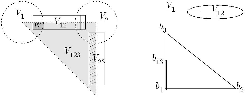
Figure 2.1. The figure on the left is schematic, showing the sets $|V_{I}|$ rather than their (disjoint) lifts $V_{I}$; the sets $V_{2,12}\subset V_{2}$ and $V_{23,123}\subset V_{23}$ are hatched, while for $x$ in the shaded set $W$, we have $I_{\min}(|x|)=\{1\},I_{1}(|x|)=\{1,2\},I_{\max}(|x|)=\{1,2,3\}$. The top right illustrates the change in dimension from $V_{1}$ to $V_{12}$, while the bottom right shows $\overline{\rm st}_{J}^{\Delta}(|x|)$ for $x\in{\widetilde{V}}_{1,123}\cap{\widetilde{V}}_{13,123}$.

The domain ${\partial}^{\prime}\,Y_{{\mathcal{V}},J,\,{\underline{{\varepsilon}}}}\subset{\partial}Y_{{\mathcal{V}},J,\,{\underline{{\varepsilon}}}}$ of the collar map $c^{Y}_{J}$ contains all the points in the image of the injections ${\iota}_{EV}$ in (2.1.11), as well as the lifts to $Y_{{\mathcal{V}},J,\,{\underline{{\varepsilon}}}}$ of all points in ${\rm im\,}(c^{Y}_{H})$ where $I\subsetneq H\subsetneq J$. To obtain points with more general $t$-coordinate we consider the following rescaling operation. Suppose given $t\in{\Delta}_{J}$ and a tuple $\mu_{J}=(\mu_{j})_{j\in A}$ such that $\mu_{j}=1$ if $j\notin J$, $\mu_{j}>0,\;\forall j$, and $\mu_{J}\cdot t\in{\Delta}_{J}$. Then for any element $(e,x;\,t)\in Y_{{\mathcal{V}},J,\,{\underline{{\varepsilon}}}}$, there is a commutative diagram

(2.1.21)

where we assume $\|(\mu_{J})^{-1}\cdot e\|<{\kappa}\,{\varepsilon}_{I(x)}$ so that the top arrow has target in $Y_{{\mathcal{V}},J,\,{\underline{{\varepsilon}}}}$.

The following result concerns a reduction ${\mathcal{V}}$ plus choice of constants ${\underline{{\varepsilon}}}$ that are compatible in the sense of Definition 3.1.9. In particular this means that property (i) in Proposition 2.1.1 holds, and that $({\mathcal{V}},{\underline{{\varepsilon}}})$ is compatible with a fixed choice of local product structures as in (1.2.3). The proof is given in Lemma 3.2.1 below.

Proposition 2.1.4.

Let $({\mathcal{V}},\,{\underline{{\varepsilon}}})$ be a compatible reduction of an atlas ${\mathcal{K}}$. Then for each $J\in{\mathcal{I}}_{\mathcal{K}}$ there is an open subset ${\partial}^{\prime}\,Y_{{\mathcal{V}},J,\,{\underline{{\varepsilon}}}}\subset{\partial}\,Y_{{\mathcal{V}},J,\,{\underline{{\varepsilon}}}}$, a constant $w_{J}>0$, and a ${\Gamma}_{A}$-equivariant embedding

(2.1.22) $$c_{J}^{Y}:{\partial}^{\prime}\,Y_{{\mathcal{V}},J,\,{\underline{{\varepsilon}}}}\times[0,w_{J})\to Y_{{\mathcal{V}},J,\,{\underline{{\varepsilon}}}},\quad\bigl{(}(e,x;t),r\bigr{)}\mapsto(e^{\prime},x^{\prime};c_{J}^{\Delta}(t,r)),$$

with the following properties:

• ${\partial}^{\prime}\,Y_{{\mathcal{V}},J,\,{\underline{{\varepsilon}}}}\subset\bigl{\{}(e,x;t):\exists I\subsetneq J,x^{0}\in{\widetilde{V}}_{IJ},\mbox{ s.t.}\;\;x\approx x^{0},\ t\in\overline{\rm st}^{\Delta}_{J}(|x^{0}|)\bigr{\}}$,

• $c_{J}^{Y}$ is compatible with the projections to $E_{A{\smallsetminus}\bullet}$ as follows: we have

  (2.1.23) $${\iota}_{EV}(E_{A{\smallsetminus}I,{\varepsilon}_{I}}\times{\widetilde{V}}_{IJ})\;\subset\;{\partial}^{\prime}\,Y_{{\mathcal{V}},J,\,{\underline{{\varepsilon}}}},\quad\forall\,\,I\subsetneq J.$$

  Further,

  (2.1.24) $$c_{J}^{Y}\bigl{(}(e,x;t),0\bigr{)}=(e,x;t),\quad\forall(e,x;t)\in{\partial}^{\prime}\,Y_{{\mathcal{V}},J,\,{\underline{{\varepsilon}}}},$$

  $${\rm pr}_{E_{J{\smallsetminus}I}}(e)=0\;\;\Longrightarrow\;\;c_{J}^{Y}\bigl{(}(e,x;t),r\bigr{)}=\bigl{(}e,x;c^{\Delta}_{J}(t,r)\bigr{)},\mbox{ and }$$

  (2.1.25) $${\rm pr}_{E_{A{\smallsetminus}I}}\circ c_{J}^{Y}\bigl{(}{\iota}_{EV}(e,x),r\bigr{)}={\rm pr}_{E_{A{\smallsetminus}I}}(e),\quad\forall(e,x)\in E_{A{\smallsetminus}I,{\varepsilon}_{I}}\times{\widetilde{V}}_{IJ},$$

• the sets ${\partial}^{\prime}\,Y_{{\mathcal{V}},J,\,{\underline{{\varepsilon}}}}$ are compatible with covering maps as follows: if $I\subsetneq H\subsetneq J$, then the relevant part of the image of $c^{Y}_{H}$ lifts to the domain ${\partial}^{\prime}\,Y_{{\mathcal{V}},J,\,{\underline{{\varepsilon}}}}$ of $c^{Y}_{J}$. More precisely, if $(e,x;t)\in{\partial}^{\prime}\,Y_{{\mathcal{V}},J,\,{\underline{{\varepsilon}}}}$ has $x\in\rho_{HJ}^{-1}({\widetilde{V}}_{IH})\cap{\widetilde{V}}_{HJ}$ and $t\in{\partial}_{H{\smallsetminus}I}{\Delta}_{H}$, then $(e,\rho_{HJ}(x);\,t)$ is in the domain ${\partial}^{\prime}\,Y_{{\mathcal{V}},H,\,{\underline{{\varepsilon}}}}$ of $c^{Y}_{H}$ and for all $r\in[0,w_{H})$ there is $(e^{\prime},x^{\prime};\,t^{\prime})\in{\partial}^{\prime}\,Y_{{\mathcal{V}},J,\,{\underline{{\varepsilon}}}}$ with $x^{\prime}\in{\widetilde{V}}_{HJ}$ such that

  (2.1.26) $$c^{Y}_{H}((e,x;t),r)=\bigl{(}e^{\prime},\rho_{HJ}(x^{\prime});\,t^{\prime}\bigr{)}\;\in\;Y_{{\mathcal{V}},H,{\underline{{\varepsilon}}}}.$$

  Further, the restriction of $c^{Y}_{H}$ to $Y_{{\mathcal{V}},H,\,{\underline{{\varepsilon}}}}\cap{\rm pr}_{V}^{-1}({\widetilde{V}}_{IH}\cap V_{HJ})$ has a well defined lift (also called $c^{Y}_{H}$) to $Y_{{\mathcal{V}},J,\,{\underline{{\varepsilon}}}}$ such that for all $x\in{\widetilde{V}}_{IJ}\cap{\widetilde{V}}_{HJ}$

  (2.1.27) $$({\rm pr}^{Y}_{HJ})_{*}\bigl{(}c^{Y}_{H}(e,x;t),r\bigr{)}=\bigl{(}c^{Y}_{H}(e,\rho_{HJ}(x),t),r\bigr{)}\;\in\;Y_{{\mathcal{V}},H,{\underline{{\varepsilon}}}},\quad r\in[0,w_{H}),$$

  where $({\rm pr}^{Y}_{HJ})_{*}$ is as in (2.1.12).

• each ${\partial}^{\prime}\,Y_{{\mathcal{V}},J,\,{\underline{{\varepsilon}}}}$ is invariant under rescaling as follows: if $(e,\,x;\,t)\in{\partial}^{\prime}\,Y_{{\mathcal{V}},J,\,{\underline{{\varepsilon}}}}$ where $t\in\overline{\rm st}_{H}^{\Delta}(|x|)$ then for all $\mu_{H}$ as in (2.1.21) such that $\mu_{H}\cdot t\in\overline{\rm st}_{H}^{\Delta}(|x|)$ we have

  $$\mu_{H}\cdot\bigl{(}e,x;\,t\bigr{)}:=\bigl{(}\mu_{H}^{-1}\cdot e,x;\,\mu_{H}\cdot t\bigr{)}\in{\partial}^{\prime}\,Y_{{\mathcal{V}},J,\,{\underline{{\varepsilon}}}}$$

  and

  (2.1.28) $${\rm pr}_{E_{A{\smallsetminus}H}\times V}\circ c^{Y}_{J}\bigl{(}(e,\,x;\,t),r\bigr{)}=$$

  $$\qquad{\rm pr}_{E_{A{\smallsetminus}H}\times V}\circ c^{Y}_{J}\bigl{(}(\mu_{H}^{-1}\cdot e,x;\,\mu_{H}\cdot t),r\bigr{)}\in E_{A{\smallsetminus}H}\times V_{J};$$

• the collar maps $c^{Y}_{J}$ are compatible with shrinkings as follows: if $({\mathcal{V}}^{\prime},{\underline{{\varepsilon}}}^{\prime})\sqsubset({\mathcal{V}},{\underline{{\varepsilon}}})$ is another compatible reduction, then there are constants $0<w_{J}^{\prime}<w_{J}$ such that the restrictions of the maps $c^{Y}_{J}$ to ${\partial}^{\prime}\,Y_{{\mathcal{V}}^{\prime},J,\,{\underline{{\varepsilon}}}^{\prime}}:={\partial}Y_{{\mathcal{V}}^{\prime},J,\,{\underline{{\varepsilon}}}^{\prime}}\cap{\partial}^{\prime}\,Y_{{\mathcal{V}},J,\,{\underline{{\varepsilon}}}}$ have all the above properties with respect to the constants $w_{J}^{\prime}$.

• if ${\mathcal{K}}$ is oriented then the collar map $c^{Y}_{J}$ is compatible with the natural induced orientation on its domain and range.

By Lemma 3.1.11, any reduction ${\mathcal{V}}^{\prime\prime}$ has a shrinking ${\mathcal{V}}\sqsubset{\mathcal{V}}^{\prime\prime}$ that is compatible with respect to some choice of constants ${\underline{{\varepsilon}}}$ and hence supports a collar $\bigl{(}c^{Y}_{J}\bigr{)}_{J\in{\mathcal{I}}_{\mathcal{K}}}$ as in Proposition 2.1.4. Further, we show in Corollary 3.2.3 that $({\mathcal{V}}^{\infty},{\underline{{\varepsilon}}}^{\infty})$ has a further nested shrinking that is collar compatible in the following sense.

Definition 2.1.5.

Let $({\mathcal{V}}^{\infty},{\underline{{\varepsilon}}}^{\infty})$ be a compatible reduction, with collars $\bigl{(}c^{Y,\infty}_{J}\bigr{)}_{J\in{\mathcal{I}}_{\mathcal{K}}}$. We say that a shrinking $({\mathcal{V}},{\underline{{\varepsilon}}})\sqsubset({\mathcal{V}}^{\infty},{\underline{{\varepsilon}}}^{\infty})$ is collar compatible if it is compatible as in Definition 3.1.9 and if for all $J\in{\mathcal{I}}_{\mathcal{K}}$ the collar map $c^{Y,\infty}_{J}$ restricts to a collar $(c^{Y}_{J})_{J}$ on $({\mathcal{V}},{\underline{{\varepsilon}}})$ whose widths $w_{J}$ satisfy $\sqrt{{\varepsilon}_{I}}<w_{J}$ for all $I\subsetneq J$.

2.2. Construction of the category ${\bf M}$ and functor ${\mathscr{S}}:{\bf M}\to{\bf E}_{A}$

In (1.3.5), the component $M_{J}$ of ${\rm Obj}_{\bf M}$ was defined as

(2.2.1) $$M_{J}=E_{A{\smallsetminus}J,{\varepsilon}_{J}}\times V_{J},$$

which is a manifold of dimension $d+\dim E_{A}$. We take $M_{IJ}:=E_{A{\smallsetminus}J,{\varepsilon}_{J}}\times V_{IJ}$, and define the map $\tau_{IJ}:{\widetilde{M}}_{IJ}\to M_{IJ}$ that attaches $M_{J}$ to $M_{I}$ to have domain a suitable open subset ${\widetilde{M}}_{IJ}\subset M_{J}$ and to extend the atlas structural map

$$\rho_{IJ}:\{0\}\times{\widetilde{V}}_{IJ}\to\{0\}\times V_{IJ}\subset M_{IJ}\subset M_{I}.$$

We require that $\tau_{IJ}$ is a ${\Gamma}_{A}$-equivariant covering map, induced by a free action of ${\Gamma}_{J{\smallsetminus}I}$. Further, to obtain a category, these maps must be compatible with composition: i.e. for $I\subset H\subset J$ we need

(2.2.2) $$\tau_{HJ}\circ\tau_{IH}=\tau_{IJ}\;\;\mbox{ on }\;\;{\widetilde{M}}_{IJ}\cap{\widetilde{M}}_{HJ}\cap\tau_{HJ}^{-1}({\widetilde{M}}_{IH})={\widetilde{M}}_{IJ}\cap{\widetilde{M}}_{HJ}.$$

(Note that by (1.3.3) any two of the sets ${\widetilde{M}}_{IJ},{\widetilde{M}}_{HJ},\tau_{HJ}^{-1}({\widetilde{M}}_{IH})$ determine the third.) For maximal elements $J$ of ${\mathcal{I}}_{\mathcal{K}}$, we then define ${\mathscr{S}}_{J}:M_{J}\to E_{A}$ as the projection

$${\mathscr{S}}_{J}:M_{J}\to E_{A},\quad (e_{A{\smallsetminus}J},x)\mapsto(e_{A{\smallsetminus}J},s_{J}(x)).$$

The above should be considered as the default formula for ${\mathscr{S}}_{J}$, that holds at points $(e_{A{\smallsetminus}J},x)\in M_{J}$ where $x$ is far from any overlap $V_{JK}$ with $J\subsetneq K$. However, in general it must be modified in ways explained in Example 2.2.1 below.

Before giving the general formulas for $\mu_{J},\tau_{IJ},{\mathscr{S}}_{J}$, we discuss an example. Part (i) shows the role of the collar in constructing $\tau_{IJ}$, and also how to achieve the closed graph condition in (1.3.6), while part (ii) explains the relevance of the collar’s compatibility with projections and rescaling to the proof of the composition rule (2.2.2). The usefulness of considering multiple collar compatible shrinkings $({\mathcal{V}}^{n},{\underline{{\varepsilon}}}^{n})$ will also become apparent. We will use cutoff functions $\bigl{(}\chi_{IJ}:V_{I}\to[0,1]\bigr{)}_{I\subsetneq J}$ of the following form: if ${\mathcal{V}}\sqsubset{\mathcal{V}}^{\prime}$ we have

(2.2.3) $${\textstyle{\rm supp\,}(\chi_{IJ})\subset\bigcup_{I\subsetneq H\subset J}V_{IH}^{\prime},\quad\mbox{ and }\;\;\bigcup_{I\subsetneq H\subset J}\overline{V}_{IH}\subset{\rm int\,}(\chi_{IJ}^{-1}(1)).}$$

Example 2.2.1.

(Attaching the $M_{J}$).  We begin by considering the case when the isotropy groups are trivial, so that $\tau_{IJ}:{\widetilde{M}}_{IJ}\to M_{IJ}$ is a homeomorphism. It is then easiest to define its inverse

$${\alpha}_{IJ}:=\tau^{-1}_{IJ}:M_{IJ}\to{\widetilde{M}}_{IJ},$$

since $M_{IJ}\subset M_{I}$ is defined to be the product $E_{A{\smallsetminus}I,{\delta}_{I}}\times V_{IJ}$ (where $V_{IJ}$ is defined in (1.3.3)) while ${\widetilde{M}}_{IJ}$ will simply be defined as the image ${\alpha}_{IJ}(M_{IJ})$. As in [MW2], we use the notation $\phi_{IJ}:=\rho_{IJ}^{-1}:V_{IJ}\to{\widetilde{V}}_{IJ}$ for the inverse of the atlas structural map $\rho_{IJ}$.

(i) Consider the case when there are two basic charts with labels $1,2$. Then ${\bf M}$ has three components:

$$M_{1}=E_{2,{\delta}_{2}}\times V_{1},\quad M_{2}=E_{1,{\delta}_{1}}\times V_{2},\quad M_{12}:=V_{12},$$

where we assume $({\mathcal{V}},{\underline{{\delta}}})$ is collar compatible as in Definition 2.1.5. In particular, this means that for $i=1,2$ we have ${\delta}_{i}<w_{12}^{2}$, where $w_{12}$ is the width of the collar $c^{Y}_{12}$. We first define the attaching maps ${\alpha}_{1,12}$ and ${\alpha}_{2,12}$, then define the sections ${\mathscr{S}}_{I}$. and finally prune the sets $M_{12}$ so as to satisfy the closed graph condition.

We define ${\alpha}_{1,12}$ as a composite $M_{1,12}:=E_{2,{\delta}_{2}}\times V_{1,12}\;\to\;Y_{{\mathcal{V}},12,{\underline{{\delta}}}}\;\to\;M_{12}$:

$${\alpha}_{1,12}\bigl{(}(e_{2},x)\bigr{)} ={\rm pr}_{V}\Bigl{(}c_{12}^{Y}\bigl{(}{\iota}_{EV}(e_{2},x),\,r\bigr{)}\Bigr{)}\;\;\mbox{ with }r:=\sqrt{\|e_{2}\|}$$

(2.2.4) $$={\rm pr}_{V}\Bigl{(}c_{12}^{Y}\bigl{(}(s_{1}(x),e_{2},\phi_{IJ}(x);b_{1}),r\bigr{)}\Bigr{)}\;\;$$

$$={\rm pr}_{V}\Bigl{(}\bigl{(}e_{1}^{\prime},e_{2},x^{\prime};(1-\ r,r)\bigr{)}\Bigr{)},\;\;$$

$$=x^{\prime}\in V_{12}=M_{12},$$

where ${\iota}_{EV}$ is the map in (2.1.11), $b_{1}=(1,0)$ is the barycenter of ${\Delta}_{1}$ considered as a point in ${\Delta}_{2}$, we have used formula (2.1.13) for $c^{\Delta}_{12}$, and we have used the fact from (2.1.25) that $e_{2}$ is unchanged by $c_{12}^{Y}$. We note the following.

• Because $({\mathcal{V}},{\delta})$ is collar compatible, Definition 2.1.5 implies that the collar width satisfies $w_{12}>\sqrt{\|{\delta}_{2}\|}>r$. Hence the element $c_{12}^{Y}\bigl{(}(s_{1}(x),e_{2},\phi_{IJ}(x);b_{1}),r\bigr{)}$ is well defined for all $(e_{2},x)\in M_{1,12}$.

• Because the collar variable $r:=\sqrt{\|e_{2}\|}$ vanishes for the points $(0,x)\in M_{1,12}$, the map ${\alpha}_{1,12}$ extends the inclusion $\phi_{IJ}:V_{IJ}\to{\widetilde{V}}_{IJ}$ by (2.1.24), as is required by Proposition 1.3.3 (i). Further, for small enough ${\delta}_{i}$ the closures of the images of ${\alpha}_{1,12}$ and the similarly defined map ${\alpha}_{2,12}$ are disjoint.

• Because the points $(e,x;t)\in Y_{{\mathcal{V}},J,\,{\underline{{\varepsilon}}}}$ satisfy $s_{J}(x)=t\cdot e_{J}$ and we chose $r=\sqrt{\|e_{2}\|}$, we have

  $$r\,\|e_{2}\|=(\|e_{2}\|)^{3/2}=\|s_{2}(x^{\prime})\|,$$

  so that $r=\|s_{2}(x^{\prime})\|^{1/3}$ is determined by $x^{\prime}$.

• To see that ${\alpha}_{1,12}$ is injective, notice that because $c_{J}^{Y}$ is injective it suffices to check that the other elements, $e_{1}^{\prime},e_{2},r$ that appear in the tuple $\bigl{(}e_{1}^{\prime},e_{2},x^{\prime};(1-r,r)\bigr{)}\in Y_{{\mathcal{V}},12,\,{\underline{{\varepsilon}}}}$ are determined by $x^{\prime}\in V_{2}$. But we saw above that $r=\|s_{2}(x^{\prime})\|^{1/3}$, so that the equations $s_{1}(x)=(1-t)e_{1}^{\prime},\ s_{2}(x)=te_{2}$ determine $e_{1}^{\prime},e_{2}$.

We now define ${\mathscr{S}}_{12}:=s_{12}:M_{2}=V_{2}\to E_{12}$, and define ${\mathscr{S}}_{i}$ on ${\alpha}_{i,12}^{-1}({\widetilde{M}}_{i,12})$ by pullback: thus on this set

$${\mathscr{S}}_{i}(e_{j},x)=\bigl{(}\|e_{j}\|^{1/2}e_{j},\,s_{i}({\alpha}_{i,12}(e_{j},x)\bigr{)},\quad i\neq j,$$

has the form claimed in (1.3.7). We then extend ${\mathscr{S}}_{i}$ to the rest of $M_{i}$ by patching it to the default map $(e_{j},x)\mapsto(e_{j}\,s_{i}(x))\in E_{j}\times E_{i}=E_{12}$ via the cutoff $\chi_{i}$ in (2.2.3):

(2.2.5) $${\mathscr{S}}_{i}(e_{j},x) =\chi_{i,12}(x)\bigl{(}\|e_{j}\|^{1/2}e_{j},\,s_{i}({\alpha}_{i,12}(e_{j},x)\bigr{)}+(1-\chi_{i,12}(x))\bigl{(}e_{j},\,s_{i}(x)\bigr{)}\in E_{12}.$$

For this to be well defined, we need ${\alpha}_{i,12}$ to extend to a neighborhood of $M_{i,12}$ in $M_{i}$. But we can always assume that ${\mathcal{V}}$ is a shrinking of some other reduction ${\mathcal{V}}^{\prime}$. Then because the collar extends over ${\mathcal{V}}^{\prime}$ we may extend ${\alpha}_{i,12}$ over the corresponding set $M_{i,12}^{\prime}$ by using the above formula (2.2.1). It is then clear that ${\mathscr{S}}_{i}^{-1}(0)=\{0\}\times s_{i}^{-1}(0)$.

It remains to arrange that ${\alpha}_{i,12}$ has closed graph. Note that its restriction to $\{0\}\times V_{i,12}$ does have closed graph because ${\mathcal{V}}$ is a reduction of a good atlas ${\mathcal{K}}$, which among other things implies that the realization $|{\mathcal{V}}|\subset|{\mathcal{K}}|$ is Hausdorff; see the discussion around (1.2.7), (1.2.8). Denote by

(2.2.6) $${\rm Fr}(M_{i,12}):=cl(M_{i,12}){\smallsetminus}M_{i,12}$$

the frontier of $M_{i,12}$ in $M_{i}$, where, as usual, $cl$ denotes the closure. As above, we may assume that ${\alpha}_{i,12}$ extends to a homeomorphism ${\alpha}_{i,12}:cl(M_{i,12})\to V_{12}^{\prime}$, which evidently has a closed graph. Hence it suffices to arrange that $V_{12}\cap{\alpha}_{i,12}({\rm Fr}(M_{i,12}))=\emptyset.$ But

$$V_{12}\cap\,cl\bigl{(}{\alpha}_{i,12}({\rm Fr}(M_{i,12}))\bigr{)}\subset cl({\widetilde{V}}_{i,12}){\smallsetminus}{\widetilde{V}}_{i,12}$$

is a closed subset of $V_{12}$ that is disjoint both from $cl({\widetilde{V}}_{j,12})$ (by the separation property of the sets ${\widetilde{V}}_{1,12},{\widetilde{V}}_{2,12}$) and from the zero set $s_{12}^{-1}(0)$ (because $|{\mathcal{V}}|$ is Hausdorff). Hence, as in Figure 2.2, if this set is nonempty we can simply remove it from $V_{12}$, i.e. we replace $V_{12}$ by

(2.2.7) $$V_{12}{\smallsetminus}\textstyle{\bigcup_{i=1,2}}cl\bigl{(}{\alpha}_{i,12}({\rm Fr}(M_{i,12}))\bigr{)}.$$

Figure 2.2. Removing points from $V_{12}$ so that ${\alpha}_{i,12}$ has closed graph. Since $V_{12}$ is open the point where the two heavy lines cross is not in $V_{12}$. The set ${\widetilde{M}}_{i,12}\;\cong\;{\widetilde{V}}_{i,12}\times E_{i,{\varepsilon}_{i}}\subset V_{12}$ is hatched.

(ii) Now suppose that the atlas ${\mathcal{K}}$ has three basic charts with labels $1,2,3$, so that the sets $V_{I}$ in the reduction ${\mathcal{V}}$ intersect as in Figure 2.1. We assume that the isotropy is trivial and all $E_{i}\neq 0$, and again explain how to choose the constants ${\delta}_{i}$, and define the attaching maps ${\alpha}_{IJ}$ and sections ${\mathscr{S}}_{I}$ that involve the vertex $1$, namely those with labels $1,12,13,$ and $123$. It is now convenient to assume that we have four nested collar compatible shrinkings $({\mathcal{V}}^{1},{\underline{{\varepsilon}}}^{1})\sqsubset({\mathcal{V}}^{2},{\underline{{\varepsilon}}}^{2})\sqsubset({\mathcal{V}}^{3},{\underline{{\varepsilon}}}^{3})\sqsubset({\mathcal{V}}^{4},{\underline{{\varepsilon}}}^{4})$ of ${\mathcal{V}}^{\prime}$. Correspondingly, with $I\subset\{1,2,3\}$ and $k\leq\ell\leq 4$ we define

$$M_{I}^{k}:=E_{I,{\varepsilon}_{i}^{k}}\times V^{k}_{I},\quad M_{IH}^{k,\ell}=E_{I,{\varepsilon}_{i}^{k}}\times V^{k,\ell}_{IH}\;\subset\;M_{I}^{k},$$

where

$$V^{k,\ell}_{IH}=V_{I}^{k}\cap V_{IH}^{\ell}=V_{I}^{k}\cap\pi_{\mathcal{K}}^{-1}\bigl{(}\pi_{\mathcal{K}}(V_{H}^{\ell})\bigr{)}$$

We aim to define a category with basic domains of the form $M_{I}^{|I|}$ and compatible morphisms ${\alpha}_{IH}:M_{IH}^{|I|,|H|}\to M_{H}^{|H|}$. However, to make these continuous and to define the corresponding maps ${\mathscr{S}}_{I}$ we have to define transition functions on larger sets such as $M_{IH}^{|I|+1,|H|}$. As in (i), we will first define suitable maps ${\alpha}_{IH}$ and sections ${\mathscr{S}}_{I}$, and then will prune domains to achieve the closed graph condition.

If $|I|=1,|H|=2$ we define ${\alpha}_{IH}:M_{IH}^{1,2}\to M_{H}^{2}$ as in (i) above. These methods also easily adapt to define the maps ${\alpha}_{IH}$ for $|I|=2$ and ${\mathscr{S}}_{I}:M_{I}\to E_{A}$ for $|I|\geq 2$. Indeed, if $J:=\{1,2,3\}$ then

$${\alpha}_{1i,J}:M_{1i,J}^{2,3}\to M_{J}^{3}$$

can be defined much as in (2.2.1). The only new point is that because ${\Delta}_{1i}$ is a $1$-simplex, we have to decide how to lift $V_{1i,J}$ to ${\partial}Y_{{\mathcal{V}},J,\,{\underline{{\varepsilon}}}}$ in order to use the collar. For now, we use the default choice given by the embedding ${\iota}_{EV}$ in (2.1.11), i.e. we embed it over the barycenter $b_{1i}$ of ${\Delta}_{1i}$ which we identify with the corresponding point ${\iota}_{1i,J}(b_{1i})$ in ${\Delta}_{J}$. Thus with $i\neq j,\ i,j\in\{2,3\}$, we define

(2.2.8) $${\alpha}_{1i,J}: \;M_{1i,J}^{2,3}\to M_{J}^{3}:\;(e_{j},x)\mapsto x^{\prime}\;\;\mbox{ as follows: }$$

$$E_{3,{\varepsilon}^{2}_{i}}\times V_{1i}^{2,3}\ni \;(e_{j},x)\longmapsto c_{J}^{Y}\Bigl{(}\bigl{(}{\iota}_{EV}(e,x)\bigr{)},r\Bigr{)},\quad r=\sqrt{\|e_{j}\|}$$

$$=\bigl{(}e^{\prime}_{1i},e_{j},x^{\prime};c^{\Delta}_{J}(b_{1i},r)\bigr{)}\in Y_{{\mathcal{V}}^{3},J,\,{\underline{{\varepsilon}}}^{3}}$$

$$\longmapsto x^{\prime}\in M^{3}_{J}.$$

Since $r$ depends on $e_{3}$ and hence on $s_{3}(x^{\prime})$ as above, it follows as before that ${\alpha}_{1i,J}$ is injective. Notice also that if $x\in V_{1i,J}^{2,\ell}$ the point $\phi_{1i,J}(x)$ would lie in ${\widetilde{V}}^{\ell}_{1i,J}$ as would its image $x^{\prime}$ under the collar map since the collar maps preserve the shrinkings by Proposition 2.1.4. Taking $\ell=4$ here, we may therefore define ${\mathscr{S}}_{12}$ by pullback from ${\mathscr{S}}_{J}$ on $M_{12,J}^{2,3}$, tapering it off to the product $s_{12}\times{\rm pr}_{E_{j}}$ outside the larger set $E_{j,{\varepsilon}_{1i}}\times V_{1i,J}^{2,4}$ by using the cutoff functions ${\beta}_{1i,J}$ as in (2.2.5).

The main new task is to define

$${\alpha}_{1,J}:M_{1,J}^{1,3}\to M_{J}^{3},\mbox{ so that }{\alpha}_{1,J}:={\alpha}_{1i,J}\circ{\alpha}_{1,1i}\mbox{ in }M_{1,J}^{1,3}\cap M_{1,1i}^{1,2}.$$

If $x\in V_{1,J}^{1,3}{\smallsetminus}\bigcup_{i=2,3}V_{1,1i}^{1.3}$, (i.e. $x$ is “far” from $V_{1,1i}^{1,2}$) then we may define

(2.2.9) $${\alpha}_{1,J}(e_{23},x)={\rm pr}_{E_{3}\times V}\Bigl{(}c^{Y}_{J}\bigl{(}(s_{1}(x),e_{23},\ \phi_{1,J}(x),\ b_{1}),r\bigr{)}\Bigr{)},\;\;r=\sqrt{\|e_{23}\|},$$

as in (2.2.1). Hence the lift of ${\alpha}_{1,J}(e_{23},x)$ to $Y_{{\mathcal{V}}^{3},J,\,{\underline{{\varepsilon}}}^{3}}$ lies over the ray $c^{\Delta}_{J}\bigl{(}b_{1}\times[0,w_{0}]\bigr{)}\subset{\Delta}_{J}$. On the other hand, the composite ${\alpha}_{1i,J}\circ{\alpha}_{1,1i}$ first uses the collar $c^{Y}_{1i}$ for $b_{1}$ in ${\Delta}_{1i}$ and then the collar $c^{Y}_{J}$ of $b_{1i}$ in ${\Delta}_{J}$, and hence its natural lift to $Y_{{\mathcal{V}}^{3},J,\,{\underline{{\varepsilon}}}^{3}}$ is rather different. We interpolate between these two maps as follows, where we take $i=2$ for clarity, and use cut-off functions ${\beta}_{1,12}$ as in (2.2.3), with support in $V_{1,12}^{1,3}$ and that equal $1$ near the closed set $\overline{V}_{1,12}^{1,2}\sqsubset V_{1,12}^{1,3}$. Thus with $x\in V_{1,12}^{1,3}\cap V_{1,J}^{1,3}$, we define

$$(e_{23},x) \longmapsto\;c^{Y}_{12}\Bigl{(}\bigl{(}s_{1}(x),e_{23},\phi_{1,12}(x);b_{1}\bigr{)},\ r\Bigr{)}\mbox{ where }r:={\beta}_{1,12}(x)\sqrt{\|e_{2}\|}$$

$$\hskip 72.26999pt=:(e_{1}^{\prime},e_{23},x^{\prime};1-r,r)\;\in\;Y_{{\mathcal{V}}^{3},12,\,{\underline{{\varepsilon}}}^{3}}$$

(2.2.10) $$\longmapsto\;c^{Y}_{J}\bigl{(}(e_{1}^{\prime},e_{23},\phi_{12,J}(x^{\prime});\,1-r,r),r^{\prime}\bigr{)}=:\bigl{(}e_{1}^{\prime\prime},e_{23},x^{\prime\prime};t^{\prime\prime}\bigr{)}\in Y_{{\mathcal{V}}^{3},J,\,{\underline{{\varepsilon}}}^{3}}$$

$$\hskip 72.26999pt\mbox{ where }\;\;r^{\prime}:=\max\bigl{(}(1-{\beta}_{1,12}(x))\sqrt{\|e_{2}\|},\sqrt{\|e_{3}\|}\bigr{)}$$

$$\longmapsto\;x^{\prime\prime}=:{\alpha}_{1,J}\bigl{(}(e_{23},x)\bigr{)}\;\in\;M_{J}^{3}=V_{J}^{3}$$

Note the following.

• Here (as in (2.1.27)) we consider $c^{Y}_{12}$ to be the lift to ${\partial}^{\prime}\,Y_{{\mathcal{V}},J,\,{\underline{{\varepsilon}}}}$ of the collar for ${\partial}^{\prime}\,Y_{{\mathcal{V}},12,\,{\underline{{\varepsilon}}}}$, and the composite $c^{Y}_{J}\circ c^{Y}_{12}$ is defined by (2.1.26).

• The above map $(e_{23},x)\mapsto x^{\prime\prime}$ is continuous, and equals that given in (2.2.9) when ${\beta}_{1,12}(x)=0$ because $\|e_{23}\|=\max\{\|e_{i}\|:i=2,3\}$ by definition.

• If $x\in V_{1,J}^{1,3}\cap V_{1,12}^{1,2}\subset V_{1,J}^{1,3}\cap({\beta}_{1,12}^{-1}(1))$, then

  $${\alpha}_{1,12}(e_{23},x)={\alpha}_{12,J}\circ{\alpha}_{1,12}(e_{23},x).$$

  Indeed, the invariance of the collar under rescaling in (2.1.28) shows that applying the second collar map at $(1-r,r)$ with $r^{\prime}=\sqrt{\|e_{3}\|}$ and then projecting to $M_{J}^{3}$ gives the same result as rescaling, then applying the second collar at $b_{12}$ with the same $r^{\prime}$, and then projecting to $M_{J}^{3}$. Note that by (2.1.25) this last claim holds even if $e_{3}=0$, so that the second collar map has $r^{\prime}=0$ when ${\beta}_{1,12}(x)=1$.

• It remains to check that this map $(e_{23},x)\mapsto x^{\prime\prime}$ is injective. Since the first two maps in (2.2.9) are injective, it suffices to check that the projection $(e_{1}^{\prime\prime},e_{23},x^{\prime\prime};t^{\prime\prime})\to x^{\prime\prime}$ is injective. But both collar maps preserve $e_{2},e_{3}$ by the extended corner control in (2.1.25). Hence, for $i=2,3$ we know $\|e_{i}\|$ and therefore $t_{i}^{\prime\prime}$ from $s_{i}(x^{\prime\prime})=t_{i}^{\prime\prime}e_{i}$. Since $\sum_{i}t_{i}^{\prime\prime}=1$, we therefore know $t^{\prime\prime}$ and hence also $e^{\prime\prime}=(e_{1}^{\prime\prime},e_{23})$.

As before, we define ${\mathscr{S}}_{1}$ by pullback via ${\alpha}_{1,*}$ over $E_{23,{\varepsilon}_{1}}\times\bigcup_{\{1\}\subsetneq J}V_{1,J}$, extending to the rest of $M_{1}$ via a cutoff function ${\beta}_{1,J}$. However, to do this we need the pullback of ${\mathscr{S}}_{1}$ to be compatibly defined on a set that is larger than that on which we ultimately want ${\mathscr{S}}_{1}$ to equal the pullback. But we can arrange that the identity ${\alpha}_{1,J}={\alpha}_{12,J}\circ{\alpha}_{1,12}$ actually holds on a neighborhood of the closure of $V_{1,12}^{1,2}\cap V_{1,J}^{1,3}$, since in (2.2.1) ${\beta}_{1,12}=1$ on a neighborhood of $\overline{V}_{1,J}^{1,3}$, and we can always extend the domain of ${\alpha}_{1,12}$ to $V_{1,2}^{1,3}$. Therefore we can imitate the formula in (2.2.5).

It remains to prune the domains $M_{J}$ so as to achieve the closed graph condition for all maps ${\alpha}_{IJ}$. We will do this by downwards recursion on $I$. Thus, first taking $|I|=2$, we remove points from $M_{123}$ so that the maps ${\alpha}_{I,123}$ have closed graph, and then with $I=\{i\}$ remove points from all $M_{J}$ with $|J|\geq 2$ so that the maps ${\alpha}_{i,J}$ have closed graph. At each stage we use the analog of formula (2.2.7), removing from $V_{J}$ all points in ${cl}_{V_{J}}\bigl{(}{\alpha}_{IJ}({\rm Fr}(M_{IJ}))\bigr{)}$ where ${\rm Fr}(M_{IJ})$ is the frontier of $M_{IJ}=M_{IJ}^{|I|,|J|}$ in $M_{I}:=M_{I}^{|I|,|I|}$. Since ${\rm Fr}(M_{IJ})\subset M_{IJ}^{|I|,|J|+1}$, the points removed lie in the image of the extension of the collar over $Y_{J,{\mathcal{V}}^{|J|+1},\,{\underline{{\varepsilon}}}}$ but not in the image of the collar over $Y_{J,{\mathcal{V}}^{|J|},\,{\underline{{\varepsilon}}}}$. Hence, because the ${\alpha}_{IJ}$ are defined in terms of the collar map, these points do not lie in ${\rm im\,}{\alpha}_{HJ}$ for any $H\subsetneq I\subsetneq J$. Thus the different steps do not interfere with each other.

(iii) If the isotropy is nontrivial, then we can still adopt the above approach, but now must interpret ${\alpha}_{IJ}$ as a local ${\Gamma}_{x}$-invariant inverse to $\tau_{IJ}$ and then define ${\widetilde{M}}_{IJ}$ to be the ${\Gamma}_{A}$-orbit of its image. Further, we must make equivariant constructions, but this is possible since the collar is equivariant, so that all the above formulas are appropriately equivariant. In particular, the sets that must be removed in order to achieve the closed graph condition for the local inverse ${\alpha}_{IJ}$ are ${\Gamma}_{x}$-invariant, so that we can arrange that $\tau_{IJ}$ has closed graph by removing its ${\Gamma}_{A}$ orbit. ${\Diamond}$

The next result is essentially a restatement of Proposition 1.3.3, though it gives a little more information on the nature of the map $\tau_{IJ}$. Since the proof is rather complex, we describe the strategy here. As in Example 2.2.1, we define the maps ${\alpha}_{IJ}$ by downwards recursion on the cardinality $|I|$ of the index set $I$, shrinking domains at each step. In order to extend the interpolation formula for ${\alpha}_{IJ}=\tau_{IJ}^{-1}$ given in (2.2.1) to a chain of inclusions $I_{0}\subsetneq I_{1}\cdots\subsetneq I_{k}$ of length $k>1$, we apply an iterated sequence of collar maps over a family of paths ${\mathcal{P}}(e,x)$ in the simplex ${\Delta}_{J}$ as described in Step 2 below. We then define the attaching maps $\tau_{IJ}$ and ${\mathscr{S}}_{I}$, and check that they have the needed properties.

Proposition 2.2.2.

Suppose given a good atlas ${\mathcal{K}}$ on $X$. Then there is a reduction ${\mathcal{V}}$ and set of constants ${\underline{{\delta}}}=({\delta}_{I})_{I\in{\mathcal{I}}_{\mathcal{K}}}>0$, such that the following properties hold with

$$M_{I}:=E_{A{\smallsetminus}I,{\delta}_{I}}\times V_{I},\quad M_{IJ}:=E_{A{\smallsetminus}I,{\delta}_{I}}\times V_{IJ}.$$

• For each $I\subset J$ there are open sets ${\widetilde{M}}_{IJ}\subset M_{J}$ and ${\Gamma}_{A}$-equivariant maps

  $$\tau_{IJ}:{\widetilde{M}}_{IJ}\to M_{IJ}$$

  that restrict to $\rho_{IJ}$ on $\{0\}\times{\widetilde{V}}_{IJ}$ and are such that

  • ${\widetilde{M}}_{IJ}$ is a product $E_{A{\smallsetminus}J,{\delta}_{I}}\times{\widetilde{M}}^{0}_{IJ}$ where ${\widetilde{V}}_{IJ}\subset{\widetilde{M}}^{0}_{IJ}\subset V_{J}$ and $cl({\widetilde{M}}^{0}_{IJ})\cap cl({\widetilde{M}}^{0}_{HJ})=\emptyset$ unless $I,H$ are nested, and

  • $\tau_{IJ}={\rm id}_{E}\times\tau_{IJ}^{0}$ where $\tau_{IJ}^{0}:{\widetilde{M}}_{IJ}^{0}\to E_{J{\smallsetminus}I,{\delta}_{I}}\times V_{IJ}$ has the following properties:

    • $\tau_{IJ}^{0}(x)=\bigl{(}0,\rho_{IJ}(x)\bigr{)}$ for $x\in{\widetilde{V}}_{IJ}$;

    • $\tau_{IJ}^{0}$ has closed graph; and

    • $\tau_{IJ}^{0}$ quotients out by a free action of ${\Gamma}_{J{\smallsetminus}I}$ that extends to a free action on a neighborhood of $cl({\widetilde{M}}_{IJ}^{0})$ in $V_{J}$.

• for $I\subsetneq J\subsetneq K$ we have

  (2.2.11) $$\tau_{JK}({\widetilde{M}}_{IK}\cap{\widetilde{M}}_{JK}) ={\widetilde{M}}_{IJ}\cap M_{JK},\quad\mbox{ and }\;\;\tau_{IK}=\tau_{IJ}\circ\tau_{JK}.$$

• For each $J$ there is ${\mathscr{S}}_{J}:M_{J}\to E_{A}$ such that for all $J\subset K,$ we have

  (2.2.12) $${\mathscr{S}}_{J}\circ\tau_{JK}={{\mathscr{S}}_{K}}|_{{\widetilde{M}}_{JK}},\quad{\mathscr{S}}_{J}^{-1}(E_{J})\subset\{0\}\times V_{J}\;\mbox{ and }$$

  $$\qquad\qquad{\mathscr{S}}_{J}(0,x)=(0,s_{J}(x)).$$

• If the initial atlas ${\mathcal{K}}$ is oriented, then so is the category ${\bf M}$ defined by the above data as in (1.3.5).

Corollary 2.2.3.

Proposition 1.3.3 holds.

Proof.

If the category ${\bf M}$ is defined as in (1.3.5) using the above data $M_{I},{\widetilde{M}}_{IJ},\tau_{IJ}$, then all the properties of Proposition 1.3.3 hold. ∎

Proof of Proposition 2.2.2.

Step 1: The set-up and basic strategy of proof.

Fix a shrinking ${\mathcal{G}}^{0}=(G_{I}^{0})_{I\in{\mathcal{I}}_{\mathcal{K}}}$ of the footprint cover. By Corollary 3.2.3 we may choose a family of nested collar compatible shrinkings as above

$$\psi^{-1}({\mathcal{G}}^{0})\sqsubset({\mathcal{V}}^{1},\,{\underline{{\varepsilon}}}^{1})\sqsubset\cdots\sqsubset({\mathcal{V}}^{{\kappa}+1},\,{\underline{{\varepsilon}}}^{{\kappa}+1})\sqsubset({\mathcal{V}}^{\infty},\,{\underline{{\varepsilon}}}^{\infty})\sqsubset{\mathcal{U}}^{\infty},$$

with collar widths that increase with $m$. The projection $\pi_{\mathcal{K}}:U_{I}^{\infty}\to|{\mathcal{K}}|$ quotients out by ${\Gamma}_{I}$ and its restrictions to the ${\mathcal{V}}^{m}$ have the property that

$$\pi_{\mathcal{K}}(\overline{V^{k}_{I}})\cap\pi_{\mathcal{K}}(\overline{V_{J}^{\ell}})\neq\emptyset\;\Longleftrightarrow\;I\subset J\mbox{ or }J\subset I.$$

For $m\leq\ell$ we denote $V^{m,\ell}_{IJ}:=V_{I}^{m}\cap\pi_{\mathcal{K}}^{-1}(\pi_{\mathcal{K}}(V^{\ell}_{J}))$, and for $m\leq|I|,\;m\leq\ell\leq|J|$ define

(2.2.13) $$M_{I}^{m}:=E_{A{\smallsetminus}I,{\varepsilon}_{I}^{m}}\times V_{I}^{m},\qquad M_{IJ}^{m,\ell}=E_{A{\smallsetminus}I,{\varepsilon}_{I}^{m}}\times V_{IJ}^{m,\ell}.$$

For each $I\subsetneq J$ and $m\leq|I|$ we will define ${\mathscr{S}}_{J}:M_{J}^{|J|}\to E_{A}$, a subset ${\widetilde{M}}_{IJ}^{m,\ell}\subset M_{J}^{\ell}$ and a ${\Gamma}_{A}$-equivariant covering map

$$\tau^{m,\ell}_{IJ}:{\widetilde{M}}_{IJ}^{m,\ell}\to M_{IJ}^{m,\ell}$$

with the following properties:

• $\tau^{m,\ell}_{IJ}$ has product form and closed graph as in (i), and quotients out by a free action of ${\Gamma}_{J{\smallsetminus}I}$ on $({\widetilde{M}}_{IJ}^{m,\ell})^{0}$;

• for all $m\leq m^{\prime}\leq|I|,\ell\leq\ell^{\prime}\leq|J|$, ${\widetilde{M}}_{IJ}^{m,\ell}\subset{\widetilde{M}}_{IJ}^{m^{\prime},\ell^{\prime}}$ and $\tau^{m^{\prime},\ell^{\prime}}_{IJ}|_{{\widetilde{M}}_{IJ}^{m,\ell}}=\tau^{m,\ell}_{IJ}$;

• if $I\subsetneq H\subsetneq J$ then $\tau_{IJ}^{|I|,|J|}=\tau_{HJ}^{|H|,|J|}\circ\tau_{IH}^{|I|,|H|}$ on their common domain; moreover this domain maps onto

  $$E_{A{\smallsetminus}I,{\varepsilon}_{I}}\times\Bigl{(}V_{IJ}^{|I|,|J|}\cap\rho_{IJ}(V_{HJ}^{|H|,|J|})\Bigr{)}\subset M_{I}^{|I|}.$$

• if $I\subsetneq J$ then ${\mathscr{S}}_{I}\circ\tau_{IJ}={\mathscr{S}}_{J}$ on ${\widetilde{M}}_{IJ}^{|I|,|J|}$;

• ${\mathscr{S}}_{J}^{-1}(0)=\{0\}\times s_{J}^{-1}(0)\subset M_{J}^{|J|}$.

In the end we will take

$$M_{I}:=M_{I}^{|I|},\quad M_{IJ}:=M_{IJ}^{|I|,|J|}$$

with the corresponding sets ${\widetilde{M}}_{IJ}^{|I|,|J|}$, and the restrictions of the maps $\tau_{IJ}$ and ${\mathscr{S}}_{I}$. In particular, ${\delta}_{I}={\varepsilon}_{I}^{|I|}$.

For simplicity, we first assume that the isotropy groups are trivial. As in Example 2.2.1 (see in particular (2.2.1)) for $I\subsetneq J$ we will define a family of injective maps

$${\alpha}_{IJ}:M_{IJ}^{|I|+1,|J|+1}\cap\{(e,x)\,\big{|}\;\|e_{J{\smallsetminus}I}\|<{\varepsilon}_{I}^{|I|}\}\;\;\to\;\;M_{J}^{|J|+1},\quad{\lambda}\geq 1$$

(where $e_{J{\smallsetminus}I}:={\rm pr}_{E_{J{\smallsetminus}I}}(e)$) with well defined restrictions

(2.2.14) $${\alpha}_{IJ}:={\alpha}_{IJ}\big{|}_{M_{IJ}^{m,k}}:M_{IJ}^{m,k}\to M_{J}^{k},\quad m\leq|I|+1,k\leq|J|+1,m\leq k,$$

such that

(2.2.15) $${\alpha}_{IJ}={\alpha}_{HJ}\circ{\alpha}_{IH}\mbox{ on }M_{IJ}^{|I|,|J|}\cap{\alpha}_{IH}^{-1}(M_{HJ}^{|H|,|J|}),\quad\forall\;I\subsetneq H\subsetneq J.$$

Then we define

$${\widetilde{M}}_{IJ}^{m,\ell}={\alpha}_{IJ}(M_{IJ}^{m,\ell}),\quad\tau_{IJ}={\alpha}_{IJ}^{-1}.$$

With this, conditions (b), (c) will hold and $\tau_{IJ}={\alpha}_{IJ}^{-1}$ has the required product form. We will arrange the rest of (a) later.

Step 2: Definition of ${\alpha}_{IJ}$ via the paths ${\mathcal{P}}(e,x)$.

Figure 2.3. The path ${\mathcal{P}}(e,x)$ with $I_{k}=\{1\},\dots,I_{k+3}=\{1,2,3,4\}$.

To define ${\alpha}_{IJ}(e,x)$ we consider the chain of length $m=m(|x|)$ formed by the sets $H$ such that $|x|\in|V_{H}|^{|H|+1}$

(2.2.16) $$I_{\min}(|x|)=I_{0}(|x|)\subsetneq I_{1}(|x|)\subsetneq\cdots\subsetneq I_{m}(|x|)=I_{\max}(|x|),$$

modifying the definition of $\overline{\rm st}^{\Delta}_{J}(|x|)$ from (2.1.16) accordingly. Extending the procedure in (2.2.1), if $I=I_{k}(|x|)$ we define ${\alpha}_{IJ}(e,x)$ by applying collar maps in $Y_{{\mathcal{V}}^{{\kappa}+1},I_{m},{\underline{{\varepsilon}}}^{{\kappa}+1}}$ a total of $m-k$ times with initial points $p_{n-1}\in{\rm pr}_{\Delta}^{-1}({\Delta}_{I_{n}})$ and collar lengths $r_{n}$ for $n=k+1,\dots,m=m(|x|)$. In fact, it is useful to think of applying the iterated collar map that lies over the path ${\mathcal{P}}(e,x)$ in $\overline{\rm st}^{\Delta}_{J}(|x|)$ with the following vertices:

$$p_{k}=b_{I_{k}},\;\;p_{n}=(1-r_{n})p_{I_{n-1}}+r_{n}b_{I_{n}}=c_{I_{n}}^{\Delta}(p_{n-1},r_{n}),\quad k<n\leq m(|x|),$$

(see Figure 2.3) where the $r_{n}$ are described below. Note that by the collar compatibility with covering maps in (2.1.27) it makes no difference whether at the $n$th step we apply the collar map over the segment $[p_{n-1},p_{n}]$ in $Y_{{\mathcal{V}},I_{n},{\underline{{\varepsilon}}}}$ (where ${\mathcal{V}}:={\mathcal{V}}^{\kappa}$) and then lift to the next level $Y_{{\mathcal{V}},I_{n+1},{\underline{{\varepsilon}}}}$, or whether we first lift all the way to $Y_{{\mathcal{V}},I_{m},{\underline{{\varepsilon}}}}$ (where $I_{m}=I_{\max}$), and then apply the collar maps. We take the second approach, first lifting the initial point $(e_{A{\smallsetminus}I_{k}},x)$ to

$$(e_{A{\smallsetminus}I_{k}}+b_{I_{k}}^{-1}\cdot s_{I_{k}}(x),\,\phi_{I_{k}I_{m}}(x);b_{I_{k}})\in{\partial}_{I_{m}{\smallsetminus}I_{k}}Y_{{\mathcal{V}},I_{m},{\underline{{\varepsilon}}}^{{\kappa}+1}}\cap{\partial}^{\prime}_{I_{m}{\smallsetminus}I_{0}}Y_{{\mathcal{V}},I_{m},{\underline{{\varepsilon}}}^{{\kappa}+1}}$$

and then applying successive collar maps that remain in the boundary ${\partial}^{\prime}\,Y_{{\mathcal{V}},I_{m},{\underline{{\varepsilon}}}^{{\kappa}+1}}$ until the very last step. Note that by the collar compatibility with shrinkings we can work in ${\mathcal{V}}:={\mathcal{V}}^{\kappa}$ rather than in the different ${\mathcal{V}}^{i}$.

To complete this definition of ${\alpha}_{IJ}(e_{A{\smallsetminus}I},x)$ it remains to define the lengths $r_{n}=r_{n}(x)$ for $k+1\leq n\leq m$. To achieve consistency with coordinate changes, for each $I\in{\mathcal{I}}_{\mathcal{K}}$, we choose a cutoff function $\chi_{I}:|{\mathcal{K}}|\to[0,1]$ such that

(2.2.17) $${\rm supp\,}(\chi_{I})\subset\pi_{\mathcal{K}}(V_{I}^{|I|+1}),\qquad\chi_{I}^{-1}(1)\subset\pi_{\mathcal{K}}(V_{I}^{|I|}),$$

and for each $J$ denote its pullback to the set $V_{J}^{|J|+1}$ by the same letter. Then, writing $a_{n}:=\sqrt{\|e_{I_{n}{\smallsetminus}I_{n-1}}\|}$ and $\chi_{i}:=\chi_{I_{i}}$, we define

$$r_{m+1}(x): =\chi_{{m+1}}(x)a_{m+1},\;\;r_{m+2}(x)=\chi_{{m+2}}(x)\max\bigl{(}(1-\chi_{{m+1}}(x))a_{m+1},a_{m+2}\bigr{)},\dots$$

$$r_{n}(x): =\chi_{n}(x)\Bigl{(}\max_{m<j\leq n}{\lambda}_{j}a_{j}\Bigr{)},\quad{\lambda}_{j}:=\prod_{i=j}^{n-1}(1-\chi_{i}(x)),\;\;j<n,\;\;{\lambda}_{n}:=1.$$

To check that ${\alpha}_{IJ}(e_{A{\smallsetminus}I},x)$ is well defined we note the following.

• The path ${\mathcal{P}}(e,x)$ depends both on the position of $|x|$ with respect to the sets $|V_{H}|^{|H|+1}$ in the chain (2.2.16), and on the relative sizes $a_{k}$ of the relevant components of $e$; cf. equations (2.2.1).

• In order for the collar maps to be defined over ${\mathcal{P}}(e,x)$, we must have $r_{n}(x)<w_{I_{n}}$ for all $n$. But

  $$r_{n}\leq\max_{m<j\leq n}\sqrt{\|e_{I_{n}{\smallsetminus}I_{n-1}}\|}<\sqrt{\|e_{A{\smallsetminus}I}\|}<\sqrt{{\varepsilon}_{I_{m}}}<w_{I_{n}}$$

  for all $m>n$ because $({\mathcal{V}},{\underline{{\varepsilon}}})$ is collar compatible: see Definition 2.1.5.

• Further at each stage we need the image of the iterated collar map to lie in the domain of the next collar map It follows from (2.1.23) that the initial point

  $$(e_{A{\smallsetminus}I_{k}}+b_{I_{k}}^{-1}\cdot s_{I_{k}}(x),\,\phi_{I_{k}I_{m}}(x);b_{I_{k}})$$

  of ${\mathcal{P}}(e,x)$ does lie in ${\partial}^{\prime}\,Y_{{\mathcal{V}},J,\,{\underline{{\varepsilon}}}}$. One then uses the fact that these domains ${\partial}^{\prime}\,Y_{{\mathcal{V}},J,\,{\underline{{\varepsilon}}}}$ are compatible with covering maps, as explained in (2.1.26),(2.1.27).

• To see that the path ${\mathcal{P}}(e,x)$ varies continuously with $x$, it suffices to check continuity for a sequence of points $x^{\nu}\to x^{\infty}$ for which just one of the functions $\chi$ — say $\chi_{s}$ — changes from a positive value to zero. But in this case (assuming that $e$ is fixed) the functions $r_{i}(x)$ are continuous for $i<s$, while for $i\geq s$ we have

  $$a_{i}^{\nu}=a_{i}^{\infty},i\neq s,s+1,\quad a_{s}^{\infty}=\max(a_{s}^{\nu},a_{s+1}^{\nu}),$$

  $$\lim_{\nu}r_{i}(x^{\nu})=r_{i}(x^{\infty}),i<s,\quad\lim_{\nu}r_{s}(x^{\nu})=0,\quad\lim_{\nu}r_{i}(x^{\nu})=r_{i-1}(x^{\infty}),i>s.$$

• If $x\in V_{IH}^{|I|+1,|H|}$ for $H=I_{s}$ where $m<s<n$, then $\chi_{s}(x)=1$. In this case, we can divide ${\mathcal{P}}(e,x)$ into two independent segments at the point $p_{s}$, because the lengths $r_{n}(x),n>s$ no longer depend on $a_{i},i\leq s$ since ${\lambda}_{i}=0$ for $i\leq s$. Further, the second part of ${\mathcal{P}}(e,x)$ projects to the path ${\mathcal{P}}(\phi_{IH}(x))$ under the natural projection

  $$\bigl{(}{\rm conv}(b_{I_{0}},\dots,b_{I_{\max}(|x|)})\bigr{)}{\smallsetminus}\bigl{(}{\rm conv}(b_{I_{0}},\dots,b_{I_{s}})\bigr{)}\;\to\;{\rm conv}(b_{I_{s}},\dots,b_{I_{\max}}).$$

Step 3: Definition of the maps ${\alpha}_{IJ}$ and sections ${\mathscr{S}}_{I}$ in the case of trivial isotropy.

With these formulas in hand, we now define the maps ${\alpha}_{IJ}$ and sections ${\mathscr{S}}_{I}$ by downwards recursion on $|I|$. For $|J|={\kappa}:=\max\{|J|:J\in{\mathcal{I}}_{\mathcal{K}}\}$, we define

$${\mathscr{S}}_{J}: ={\mathscr{S}}_{J}^{\prime},\quad\mbox{ where }$$

$${\mathscr{S}}_{J}^{\prime}: \;M_{J}\to E_{A},\quad(e_{A-J},x)\mapsto(e_{A{\smallsetminus}J},s_{J}(x)).$$

If $|I|={\kappa}-1$, for $x\in V_{IJ}^{|I|+1,|J|}$ the path ${\mathcal{P}}(|x|)$ has one segment of length $\chi_{I}a_{k}:=\chi_{I}\sqrt{\|e_{J{\smallsetminus}I}\|}$, and we define ${\alpha}_{IJ}:M_{IJ}^{|I|,|J|}\to M_{J}^{|J|}$ by applying the collar map as in (2.2.8). For these values of $x$ we have $\chi_{I}(x)=1$. However the fact that we have defined ${\alpha}_{IJ}$ over the larger set $V_{IJ}^{|I|+1,|J|}$ means that the function

(2.2.18) $${\mathscr{S}}_{I}:=\prod_{J:I\subsetneq J}(1-\chi_{J}){\mathscr{S}}_{I}^{\prime}+\sum_{J:I\subsetneq J}\chi_{J}{\alpha}_{IJ}^{*}({\mathscr{S}}_{J}):V_{I}^{|I|}\to E_{I}.$$

is well defined and is compatible under pullback from $V_{J}$.

Let us now suppose that maps ${\alpha}_{IJ}:V_{IJ}^{|I|+1,|J|+1}\to V_{J}^{|J|+1}$, and functions ${\mathscr{S}}_{I}:V_{I}^{|I|}\to E_{A}$ have been defined for all $I\subsetneq J$ with $|I|>k$ so as to satisfy conditions (2.2.14),(2.2.15), and consider $I$ with $|I|=k$. Because there are no transition functions ${\alpha}_{II^{\prime}}$ between these sets $V_{I}$ we can work separately with each such $I$. Then define ${\alpha}_{IJ}(x)$ for $x\in V_{IJ}^{|I|+1,|J|+1}$ by applying the collar maps $c^{Y}_{HJ}$ as described in Step 2 over the part, called ${\mathcal{P}}_{IJ}(x)$ below, of the path ${\mathcal{P}}(e,x)$ from $p_{k}=b_{I}$ (where $I=I_{k}(|x|)$) to $p_{q}$, where $J=I_{q}(|x|)$.

We check the properties of ${\alpha}_{IJ}$ as follows.

• The map ${\alpha}_{IJ}$ depends continuously on $x$ because we saw above that the path ${\mathcal{P}}(e,x)$ depends continuously on $x$, and because by (2.1.25) the collar map along a path segment of length $0$ is the identity.

• Both ${\widetilde{M}}_{IJ}$ and ${\alpha}_{IJ}$ have the product form required by (a) because the collar map $c^{Y}_{J}$ does not change the components of $e_{A{\smallsetminus}I}$ that lie in $E_{A{\smallsetminus}J}$; cf. (2.1.25).

• We repeatedly use the fact that the collar is compatible with all the shrinkings to show that (b) holds.

• To prove the composition formula (c), we use the fact proved above that when $x\in M_{IH}^{|I|+1,|H|}$, the path ${\mathcal{P}}_{IJ}(x)$ divides into two independent segments, the first of which is simply ${\mathcal{P}}_{IH}(x)$, while the second projects onto ${\mathcal{P}}_{HJ}(\phi_{IJ}(x))$. Now use the invariance of the collar map under rescaling (2.1.28).

• To see that ${\alpha}_{IJ}$ is injective, notice first that the path ${\mathcal{P}}_{IJ}(x)$ is determined by $x$. Hence the collar maps applied to the lift $(e^{\prime},\phi_{IJ}(x);b_{I})$ of $(e,x)\in M_{II}$ to $Y=Y_{{\mathcal{V}},J,{\underline{{\varepsilon}}}}$ give a point in $Y$ that lies over a point $t_{x}\in{\Delta}_{J}$, that is determined by ${\mathcal{P}}(e,x)$ because the collar $c^{Y}_{J}$ lifts $c^{\Delta}_{J}$ by (2.1.22). But the collar maps are injective, as is the projection $Y_{{\mathcal{V}},J,{\underline{{\varepsilon}}}}\cap{\rm pr}_{\Delta}^{-1}(t_{x})$ to $M_{J}$.

Finally, we define ${\mathscr{S}}_{I}$ as in (2.2.18). This clearly has the properties required in (iii).

Step 4: Completion of the proof in the case of trivial isotropy. The first claims in (i), namely that $\tau_{IJ}^{0}$ extends $\rho_{IJ}$ and that ${\widetilde{M}}_{IJ}$ is a product of the form $E_{A{\smallsetminus}J,{\delta}_{I}}\times{\widetilde{M}}_{IJ}^{0}$, are clear. To establish the separation claim, namely that $cl({\widetilde{M}}^{0}_{IJ})\cap cl({\widetilde{M}}^{0}_{HJ})=\emptyset$ unless $I,H$ are nested, notice that the intersections of $cl({\widetilde{M}}^{0}_{IJ}),cl({\widetilde{M}}^{0}_{HJ})$ with $\{0\}\times V_{J}$ certainly have this property by definition of a reduction. Hence, starting with maximal $|I|$ as usual, we may, if necessary, shrink the constants ${\delta}_{I}$ so that this property holds. Further, (iv) holds, because if ${\bf K}$ is oriented, then so are all the manifolds $Y_{{\mathcal{U}},J,\,{\underline{{\varepsilon}}}}$ and $M_{I}$. Since the structural maps in ${\mathcal{K}}$ preserve orientation by definition, and the collar maps $c^{Y}_{J}$ preserve orientation by Proposition 2.1.4, so do the maps $\tau_{IJ}$ constructed above.

It remains to arrange that the maps ${\alpha}_{IJ}$ have closed graph. We do this by the method described in Example 2.2.1. Given $I\subsetneq J$, recall that $M_{IJ}:=M_{IJ}^{|I|,|J|}\subset M_{IJ}^{|I|,|J|+1}$ and define ${\rm Fr}(M_{IJ}):={cl}(M_{IJ}){\smallsetminus}M_{IJ}$ where we take the closure in $M_{IJ}^{|I|,|J|+1}$. Then the maps ${\alpha}_{IJ}$ extend to give a compatible family of embeddings defined over ${cl}(M_{IJ})$. The images ${\alpha}_{IJ}({cl}(M_{IJ})),{\alpha}_{HJ}({cl}(M_{HJ}))$ are disjoint unless $I,H$ are nested. Moreover, if $H,I$ are nested, the intersection ${\alpha}_{IJ}(M_{IJ})\cap{\alpha}_{HJ}({\rm Fr}(M_{HJ}))$ is empty because ${\alpha}_{IJ}(M_{IJ})\subset M_{J}=M_{J}^{|J|}$ while ${\alpha}_{HJ}({\rm Fr}(M_{HJ}))\subset{\rm Fr}(M_{J})\subset M_{J}^{|J|+1}{\smallsetminus}M_{J}^{|J|}$. Hence, if we define

(2.2.19) $$M_{J}^{\prime}:=M_{J}{\smallsetminus}{\textstyle\bigcup_{I\subsetneq J}}cl({\alpha}_{IJ}({\rm Fr}(M_{IJ})),$$

the maps ${\alpha}_{IJ}$ for $I\subsetneq J$ have image in $M_{J}^{\prime}$ and closed graph. Moreover, if we have already arranged that all the maps ${\alpha}_{JK}:M_{JK}\to M_{K}$ for $J\subsetneq K$ have closed graph and satisfy the compatibility conditions (2.2.15) for all $I\subset J\subset K$, then if we replace the domain $M_{JK}$ by $M_{J}^{\prime}\cap M_{JK}$ the maps ${\alpha}_{JK}:M_{JK}^{\prime}\to M_{K}$ will still have these properties. Hence we may arrange that all the maps ${\alpha}_{IJ}$ have closed graph by applying these two steps for each $J$, starting with $J$ such that $|J|$ is maximal and then working down.

This completes the proof if the isotropy groups are trivial.

Step 5: The case of nontrivial isotropy.

To construct the maps $\tau_{IJ}$ in general, we argue as above, taking $\phi_{IJ}(x)$ to be the local inverse to the covering map $\rho_{IJ}$ at $x\in{\widetilde{V}}_{IJ}$, and then defining $\tau_{IJ}$ to be the ${\Gamma}_{A}$-equivariant extension of ${\alpha}_{IJ}^{-1}$ to a neighborhood of the orbit of $(0,x)$ in ${\widetilde{M}}_{IJ}$. To see that this definition is consistent and independent of the choice of $x\in\rho_{IJ}^{-1}(\rho_{IJ}(x_{0})$, note that the collar map is equivariant and, once the shrinkings $({\mathcal{V}}^{k},{\underline{{\varepsilon}}}^{k})$ are chosen, the only other choice in the above construction is that of the cutoff functions $\chi_{I}$ in (2.2.17) whose pullbacks to the sets $V_{I}$ are also equivariant. Hence the local inverse $\phi_{IJ}(x_{0})$ is invariant under the stabilizer group ${\Gamma}_{x}$, and so the extension is well defined.

Since all the previous arguments apply without essential change, it remains to check that $\tau_{IJ}^{0}$ quotients out by a free action of ${\Gamma}_{J{\smallsetminus}I}$ on ${\widetilde{M}}_{IJ}^{0}$ that extends to a neighborhood of ${cl}({\widetilde{M}}_{IJ}^{0})$. To establish this, we must define an appropriate action of ${\Gamma}_{J{\smallsetminus}I}$ on ${\widetilde{M}}_{IJ}^{0}$. If ${\Gamma}_{J{\smallsetminus}I}$ acts trivially on $E_{J{\smallsetminus}I}$, then this action is simply the restriction of the given action of ${\Gamma}_{J{\smallsetminus}I}$ on $V_{J}$. However, in general this is not the case, and the new action

$${\Gamma}_{J{\smallsetminus}I}\times{\widetilde{M}}_{IJ}^{0}\to{\widetilde{M}}_{IJ}^{0},\quad({\gamma},x)\mapsto{\gamma}*x$$

is described as follows. Notice first that because the collar $c_{J}^{Y}$ is ${\Gamma}_{A}$-equivariant and injective, each point $x_{0}\in{\widetilde{V}}_{IJ}\subset{\widetilde{M}}_{IJ}^{0}$ with $\tau_{IJ}^{0}(x_{0})=(0,x_{0}^{\prime})\in E_{J{\smallsetminus}I,{\delta}_{I}}\times V_{IJ}$ has a neighborhood ${\mathcal{N}}(x_{0})$ on which $\tau_{IJ}^{0}$ is injective and has image ${\mathcal{N}}^{\prime}$ of product form, namely ${\mathcal{N}}^{\prime}=E_{J{\smallsetminus}I,{\delta}_{I}}\times{\mathcal{O}}^{\prime}\subset E_{J{\smallsetminus}I,{\delta}_{I}}\times V_{IJ}$. Further, ${\Gamma}_{J{\smallsetminus}I}$ acts on ${\mathcal{N}}^{\prime}$ via its action on $E_{J{\smallsetminus}I,{\delta}_{I}}$, since it fixes the points of $V_{IJ}\subset V_{I}$. If $\tau_{IJ,x_{0}}^{-1}:{\mathcal{N}}^{\prime}\to{\mathcal{N}}(x_{0})$ is the local inverse to $\tau_{IJ}$ at $x_{0}$, we now define

(2.2.20) $${\gamma}*x:={\gamma}\cdot_{J}\tau_{IJ,x_{0}}^{-1}({\gamma}^{-1}\cdot_{I}\tau_{IJ}(x)),\quad x\in{\mathcal{N}}(x_{0}).$$

where for clarity we have written $x\mapsto{\gamma}\cdot_{I}x$ (resp. $x\mapsto{\gamma}\cdot_{J}x$) for the standard action of ${\gamma}\in{\Gamma}_{J{\smallsetminus}I}$ on $E_{J{\smallsetminus}I,{\delta}_{I}}\times V_{IJ}\subset E_{J{\smallsetminus}I,{\delta}_{I}}\times V_{I}$  (resp. on ${\widetilde{M}}_{IJ}^{0}\subset V_{J}$). Then

$$\tau_{IJ}({\gamma}*x) =\tau_{IJ}\bigl{(}{\gamma}\cdot_{J}\tau_{IJ,x_{0}}^{-1}({\gamma}^{-1}\cdot_{I}\tau_{IJ}(x))\bigr{)}$$

$$={\gamma}\cdot_{I}\bigl{(}\tau_{IJ}\circ\tau_{IJ,x_{0}}^{-1}({\gamma}^{-1}\cdot_{I}\tau_{IJ}(x))\;=\;\tau_{IJ}(x),$$

where the second equality uses the equivariance of $\tau_{IJ}$ with respect to the actions $\cdot_{J},\cdot_{I}$. Now extend this action over the whole orbit by setting ${\delta}*({\gamma}*x):=({\delta}{\gamma})*x$. This new action $x\mapsto{\gamma}*x$ is free, since ${\Gamma}_{J{\smallsetminus}I}$ acts freely on ${\widetilde{V}}_{IJ}$. Further, this action extends to a free action on a neighborhood of the closure of ${\widetilde{M}}_{IJ}^{0}$ since it is determined by $\tau_{IJ}$, and hence by the collar, both of which can be extended. ∎

Lemma 2.2.4.

The action $x\mapsto{\gamma}*x$ of ${\Gamma}_{J{\smallsetminus}I}$ on ${\widetilde{M}}_{IJ}$ has the following properties:

1. if $H,I\subset J$, then the action of ${\Gamma}_{J{\smallsetminus}I}$ on ${\widetilde{M}}_{IJ}$ preserves the subset ${\widetilde{M}}_{IJ}\cap{\widetilde{M}}_{HJ}$;

2. if $H\subset I\subset J$ then the restriction to ${\widetilde{M}}_{IJ}\cap{\widetilde{M}}_{HJ}$ of the action of ${\Gamma}_{J{\smallsetminus}I}$ on ${\widetilde{M}}_{IJ}$ agrees with that obtained by considering ${\Gamma}_{J{\smallsetminus}I}$ as a subgroup of ${\Gamma}_{J{\smallsetminus}H}$ and restricting the corresponding action from ${\widetilde{M}}_{HJ}$ to ${\widetilde{M}}_{IJ}\cap{\widetilde{M}}_{HJ}$.

3. if $H\subset I\subset J$ and $y\in{\widetilde{M}}_{IJ}\cap{\widetilde{M}}_{HJ}$, then

   $$\tau_{IJ}({\gamma}_{J{\smallsetminus}H}*y)=({\gamma}_{J{\smallsetminus}H}|_{I{\smallsetminus}H})*\tau_{IJ}(y)$$

   where ${\gamma}_{J{\smallsetminus}H}|_{I{\smallsetminus}H}$ is the image of ${\gamma}_{J{\smallsetminus}H}$ under the projection ${\Gamma}_{J{\smallsetminus}H}\to{\Gamma}_{I{\smallsetminus}H}$.

4. Properties (i) and (ii) continue to hold for the extension of the action to the closure ${cl}({\widetilde{M}}_{IJ})$ of ${\widetilde{M}}_{IJ}$ in $M_{J}$.

Proof.

(i) follows from (2.2.20) because the action $x\mapsto{\gamma}\cdot_{J}x$ preserves the sets ${\widetilde{M}}_{HJ}$ for all $H\subset J$. (ii) also follows immediately from (2.2.20) and the fact that $\tau_{HJ}=\tau_{HI}\circ\tau_{IJ}$ on ${\widetilde{M}}_{IJ}\cap{\widetilde{M}}_{HJ}$. (iii) holds because the maps $\tau_{IJ}$ are equivariant with respect to the projection ${\Gamma}_{J}\to{\Gamma}_{I}$ and take ${\widetilde{M}}_{IJ}\cap{\widetilde{M}}_{HJ}$ to $M_{IJ}\cap{\widetilde{M}}_{HI}$ by (2.2.11). Finally (iv) holds because the extended action is defined by extending the domain of the maps in (2.2.20). ∎

Remark 2.2.5.

(The smooth case.) Note first that if we apply the above construction to a smooth atlas (i.e. one that satisfies the smooth submersions condition in (1.2.4)), then the charts used in (3.1.4) to give $Y_{{\mathcal{V}},J,\,{\underline{{\varepsilon}}}}$ the structure of a topological manifold do not have differentiable inverses. A related problem may also be seen in Example!2.2.1: the attaching map ${\alpha}_{1,12}$ in (2.2.1) is given by the collar, which by (3.2.3) has the form $(e_{2},x)\mapsto x^{\prime}:=\phi(\|e_{2}\|^{1/2}e_{2},x)$, where $\phi$ is the local product structure along ${\widetilde{V}}_{IJ}$ in (1.2.3). Thus, even if $\phi$ were a diffeomorphism, ${\alpha}_{1,12}$ would not have a smooth inverse along the submanifold $e_{2}=0$. Thus, just as in standard blow-up constructions, in order to obtain a smooth category ${\bf M}$ from a smooth atlas one needs to choose a smoothing of $Y_{{\mathcal{V}},J,\,{\underline{{\varepsilon}}}}$ along its boundary.

Alternatively, one could use a different construction that avoids introducing the manifold $Y$. Instead, one can construct the all important collar structure used to define the maps $\tau_{IJ}$ by using the exponential map with respect to a suitable family of metrics on the sets $V_{J}$. Indeed, recall that by the smooth tangent bundle condition (1.2.4) the derivative ${\rm d}s_{J{\smallsetminus}I}$ induces an isomorphism from the normal bundle $T^{\perp}({\widetilde{V}}_{IJ})$ of ${\widetilde{V}}_{IJ}$ in $V_{J}$ to the product $E_{J{\smallsetminus}I,{\varepsilon}_{I}}\times{\widetilde{V}}_{IJ}$. To explain the idea, let us suppose for simplicity that that the cover ${\mathcal{V}}$ is refined so that the group ${\Gamma}_{J{\smallsetminus}I}$ acts freely on the components on ${\widetilde{V}}_{IJ}$, so that the restriction of $\tau_{IJ}$ to each component is a diffeomorphism onto $V_{IJ}$ . Then we can think of $V_{IJ}$ as a subset of ${\widetilde{V}}_{IJ}$ and the task is to define a consistent family of injections ${\alpha}_{IJ}:E_{J{\smallsetminus}I,{\varepsilon}_{I}}\times V_{IJ}\to V_{J}$. To this end, choose a family of ${\Gamma}_{I}$-invariant Riemannian metrics $g_{I}$ on $V_{I}$ and constants ${\varepsilon}_{I}$ that are compatible in the following sense:

• for each $I\subsetneq J$, ${\widetilde{V}}_{IJ}$ is a totally geodesic submanifold of $(V_{J},g_{J})$ and

  $$(\rho_{IJ})_{*}(g_{J}|_{{\widetilde{V}}_{IJ}})=g_{I}|_{V_{IJ}}.$$

• $0<{\varepsilon}_{I}<{\varepsilon}_{J}$ if $I\subsetneq J$;

• for each $I\subsetneq J$, the $g_{J}$-exponential map along directions perpendicular to ${\widetilde{V}}_{IJ}$ defines an embedding ${\alpha}_{IJ}:E_{J{\smallsetminus}I,{\varepsilon}_{I}}\times V_{IJ}\to V_{J}$;

• the corners are locally flat, i.e. if $x\in{\widetilde{V}}_{IJ}\cap{\widetilde{V}}_{HJ}$ for $I\subsetneq H\subsetneq J$ then

  $${\alpha}_{IJ}\bigl{(}e_{J{\smallsetminus}H}+e_{H{\smallsetminus}I},\ x\bigr{)}={\alpha}_{HJ}\bigl{(}e_{J{\smallsetminus}H},\ {\alpha}_{IH}(e_{H{\smallsetminus}I},\ x)\bigr{)}.$$

The last condition means that the composition rule holds directly, without having to introduce analogs of the paths ${\mathcal{P}}(e,x)$. Of course, the choice of the $g_{I},{\varepsilon}_{I}$ requires some attention to detail as in the proof of Lemma 3.1.11 below; see also the construction of the perturbation section in [MW2, §7.3]. Thus one begins with a family of shrinkings ${\mathcal{V}}^{\kappa}\sqsubset\cdots\sqsubset{\mathcal{V}}^{1}\sqsubset{\mathcal{V}}^{0}$ of an initial reduction ${\mathcal{V}}^{0}$, where ${\kappa}:=\max\{|J|\ |\ J\in{\mathcal{I}}_{\mathcal{K}}\}$ and then chooses metrics $g_{J}$ on $V_{J}^{|J|}$, starting with $J$ of length $|J|=1$, that satisfy the above conditions for the submanifolds ${\widetilde{V}}_{IJ}^{|J|}$ of $V_{J}^{|J|}$ for some constant ${\varepsilon}_{I}^{\prime}>0$. Finally, once $g_{J}$ is defined on $V_{J}^{\kappa}$ for all $J$, one chooses suitable constants ${\varepsilon}_{J}$, now starting with maximal $|J|$ and working down. Further details are left to the reader, as is the proof that the resulting branched manifold is cobordant to the topological one constructed in detail above. For this last step one would need to adapt the proof of uniqueness in Step 2 of the proof of Theorem B in §2.3.

Besides obtaining a smooth rather than topological branched manifold, there are no real advantages to this construction unless one wants to work with the virtual fundamental class on the chain level using de Rham cochains. Another point is that by [M1] we can construct the branched manifold $M$ to be a simplicial complex, so that we could simplify the proof of Lemma 2.3.4 by using (locally finite) singular homology instead of Çech homology. However, because we know nothing about $X$ except that it is compact and Hausdorff, the VFC has still to be considered as an element in Çech homology. For further discussions of the smooth case, see Step 3 of the proof of Theorem B. ${\Diamond}$

2.3. Proof of Theorems A and B

To prove Theorem A, we must show that the category ${\bf M}$ constructed in §2.2 has a unique completion to a weighted branched groupoid, and then analyze the structure of this groupoid and the associated weighted branched manifold $(M,{\Lambda})$. The arguments needed here are very similar, but not identical, to those in [M3, Proposition 2.3] (which considers the case of the category ${\bf B}_{\mathcal{K}}$ defined by an atlas with trivial obstruction spaces) and in [MW3, §3.3] (which analyzes the zero set of a transverse perturbation section). Theorem B has two parts. It first states that if ${\mathcal{K}}$ is oriented the weighted branched manifold $(M,{\Lambda})$ carries a natural fundamental class $[X]^{vir}_{\mathcal{K}}$, a result that was proven in [M1] in the case when ${\bf M}$ is smooth and compact, with or without boundary. Although smoothness is assumed throughout [M1], the only place where this condition is essential is in the construction of the fundamental class in the proof of [M1, Proposition 3.25]. In this case, we may replace ${\bf M}$ by an equivalent wnb groupoid that is tame in the sense that its branching loci are piecewise smooth and hence triangulable, which allows us to work with singular homology in the proof of Lemma 2.3.4. In the present case, we must use rational Çech cohomology, and the appropriate dual homology theory for noncompact manifolds as described in §A. The second and more substantial part of the proof of Theorem B explains why $[X]^{vir}_{\mathcal{K}}$ is independent of all choices made in its construction, and why, in the smooth case, the new definition is consistent with the previous definition via perturbation sections.

We begin with a lemma about groupoid completions of étale categories; for definitions, see §1.2, §1.3. As usual we denote by ${\mathcal{I}}$ a collection of subsets of a finite set $A$, and say that $I,H\in{\mathcal{I}}$ are nested if $I\subset H$ or $H\subset I$. We state the condition identity below for completeness: it follows immediately from the fact that every category has identity morphisms.

Lemma 2.3.1.

Let ${\mathcal{I}}$ be a collection of subsets of a finite set $A$, and ${\bf M}$ be an étale category with

$${\rm Obj}_{{\bf M}} ={\textstyle\bigsqcup_{I\in{\mathcal{I}}}}M_{J},\qquad{\rm Mor}_{{\bf M}}={\textstyle\bigsqcup_{I\subset J,\,I,J\in{\mathcal{I}}}{\widetilde{M}}_{IJ}}$$

$$s\times t: \;\;{\rm Mor}_{{\bf M}}\to{\rm Obj}_{{\bf M}}\times{\rm Obj}_{{\bf M}},\quad(I,J,y)\mapsto\Bigl{(}\bigl{(}I,\tau_{IJ}(y)\bigr{)},\bigl{(}J,y\bigr{)}\Bigr{)},$$

where ${\widetilde{M}}_{IJ}\subset M_{J}$ is an open subset and the maps $\tau_{IJ}:{\widetilde{M}}_{IJ}\to M_{IJ}$ satisfy the following conditions:

• (identity) for all $I\in{\mathcal{I}}$, $\tau_{II}={\rm id}$ on ${\widetilde{M}}_{II}=M_{II}=M_{I}$;

• (composition) for all $H\subset I\subset J$, $\tau_{IJ}^{-1}({\widetilde{M}}_{HI}\cap M_{IJ})={\widetilde{M}}_{HJ}\cap{\widetilde{M}}_{IJ}$ and $\tau_{HJ}=\tau_{HI}\circ\tau_{IJ}$ on ${\widetilde{M}}_{HJ}\cap{\widetilde{M}}_{IJ}$; hence, if $z\in{\widetilde{M}}_{IJ}\cap{\widetilde{M}}_{HJ}$ where $H\subset I\subset J$ we have $(H,I,y)\circ(I,J,z)=(H,J,z).$

• (separation) ${cl}({\widetilde{M}}_{IJ})\cap{cl}({\widetilde{M}}_{HJ})=\emptyset$ unless $I,H$ are nested;

• (group actions) for each $i\in A$ there is a finite group ${\Gamma}_{i}$ such that, for all $I\subset J$, $\tau_{IJ}$ quotients out by the restriction to ${\widetilde{M}}_{IJ}$ of a free action of ${\Gamma}_{J{\smallsetminus}I}$ on $cl({\widetilde{M}}_{IJ})\subset M_{J}$, where ${\Gamma}_{J{\smallsetminus}I}:=\prod_{i\in J{\smallsetminus}I}{\Gamma}_{i}$. Moreover, these actions $x\mapsto{\gamma}*x$ satisfy the compatibility conditions listed in Lemma 2.2.4.

Then, there is a unique nonsingular groupoid $\widehat{\bf M}$ with the same object space and realization as ${\bf M}$. Its morphism spaces for $I\subset J$ are

(2.3.1) $${\rm Mor}_{\widehat{\bf M}}(M_{I},M_{J}) :={\textstyle\bigcup_{\emptyset\neq F\subset I}}\;\bigl{(}{\widetilde{M}}_{IJ}\cap{\widetilde{M}}_{FJ}\bigr{)}\times{\Gamma}_{I{\smallsetminus}F},$$

$$=\bigl{\{}(y,{\gamma})\in M_{J}\times{\Gamma}_{J}\ \big{|}\ y\in{\widetilde{M}}_{IJ},{\gamma}\in{\Gamma}_{I{\smallsetminus}H_{y}}\bigr{\}},$$

where $H_{y}:=\min\{H:y\in{\widetilde{M}}_{HJ}\}$, with

(2.3.2) $$s\times t\,(I,J,y,{\gamma}_{I{\smallsetminus}H_{y}}) =\bigl{(}\,(I,\,{\gamma}_{I{\smallsetminus}H_{y}}^{-1}*\tau_{IJ}(y)),\;(J,y)\bigr{)}$$

$$(I,I,y,{\gamma}_{I{\smallsetminus}H_{y}})^{-1} =(I,I,\,{\gamma}_{I{\smallsetminus}H_{y}}^{-1}*y,\,{\gamma}_{I{\smallsetminus}H_{y}}^{-1})$$

In particular, $\widehat{\bf M}$ is étale, and there is an injective functor ${\bf M}\to\widehat{\bf M}$.

Proof.

Observe first that because a nonsingular category has at most one morphism between any two objects, $\widehat{\bf M}$ must have precisely one morphism between any two objects $(I,x),(J,y)$ that are equivalent under the equivalence relation $\sim_{\bf M}$ on ${\rm Obj}_{{\bf M}}$ generated by ${\rm Mor}_{{\bf M}}$. Hence, there is precisely one nonsingular groupoid with ${\rm Obj}_{\widehat{\bf M}}={\rm Obj}_{{\bf M}}$ and $|\widehat{\bf M}|=|{\bf M}|$. Since there is an injection

$${\rm Mor}_{\bf M}(M_{I},M_{J})={\widetilde{M}}_{IJ}\;\hookrightarrow\;{\textstyle\bigcup_{\emptyset\neq F\subset I}}\;\bigl{(}{\widetilde{M}}_{IJ}\cap{\widetilde{M}}_{FJ}\bigr{)}\times{\Gamma}_{I{\smallsetminus}F}$$

when $I\subset J$, and the structural maps described in (2.3.2) are étale, it remains to check that the formula 2.3.1 does describe ${\rm Mor}_{\widehat{\bf M}}(M_{I},M_{J})$.

The separation property implies that for each $y\in M_{J}$ the set of $F$ such that $|y|\in|{\widetilde{M}}_{FJ}|\subset|{\bf M}|$ is nested. Let $H_{y}$ be the minimal such element. By Lemma 2.2.4, for all $H_{y}\subset I\subset J$ the group ${\Gamma}_{I{\smallsetminus}H_{y}}$ acts freely on ${\widetilde{M}}_{H_{y}I}$. Hence each element in $\bigcup_{\emptyset\neq F\subset I}\;\bigl{(}{\widetilde{M}}_{IJ}\cap{\widetilde{M}}_{FJ}\bigr{)}\times{\Gamma}_{I{\smallsetminus}F}$ has a unique description of the form $(y,{\gamma})$ where $y\in{\widetilde{M}}_{IJ},{\gamma}\in{\Gamma}_{I{\smallsetminus}H_{y}}$. Further, given such $(y,{\gamma})$ it follows from Lemma 2.2.4 (iii) that $\tau_{H_{y}J}(y)=\tau_{H_{y}I}({\gamma}^{-1}*\tau_{IJ}(y))$ for any $I$ with $y\in{\widetilde{M}}_{IJ}$, so that

$$\bigl{(}J,y\bigr{)}\sim_{\bf M}\bigl{(}H_{y},\tau_{H_{y}J}(y)\bigr{)}=\bigl{(}H_{y},\tau_{H_{y}J}({\gamma}^{-1}*\tau_{IJ}(y))\bigr{)}\sim_{\bf M}\bigl{(}I,\tau_{IJ}(y)\bigr{)}.$$

Hence for each $I$ with $y\in{\widetilde{M}}_{IJ}$ and each ${\gamma}\in{\Gamma}_{I{\smallsetminus}H_{y}}$ there must be a morphism $m$ in $\widehat{\bf M}$ from $(I,{\gamma}^{-1}*\tau_{IJ}(y))$ to $(J,y)$. To see that these are the only morphisms in $\widehat{\bf M}$ it remains to observe that each equivalence class $[(J,y)]$ contains a unique element of the form $(H_{y},z)$ where $z\in M_{H_{y}}$; further if $H_{y}\subset I\subset J$ then $[(J,y)]\cap M_{I}=\{x\in\rho_{H_{y}I}^{-1}(z)\}$ consists of the ${\Gamma}_{I{\smallsetminus}H_{y}}$-orbit of $\tau_{IJ}(y)$. Since each morphism is uniquely specified by its source and target, there is no need to write out the composition rule in $\widehat{\bf M}$ explicitly.∎

Lemma 2.3.2.

Suppose in the situation of Lemma 2.3.1 that for each $I\subset J$ the map $\tau_{IJ}$ has closed graph. Then

• the maximal Hausdorff quotient $|{\bf M}|_{\mathcal{H}}$ is the realization of a nonsingular groupoid $\widehat{\bf M}_{\mathcal{H}}$ with objects ${\rm Obj}_{{\bf M}}$ and morphisms from $M_{I}$ to $M_{J}$ with $I\subset J$ given by

  $${\rm Mor}_{\widehat{\bf M}_{\mathcal{H}}}(M_{I},M_{J}):={\textstyle\bigcup_{\emptyset\neq F\subset I}}\;\bigl{(}{\widetilde{M}}_{IJ}\cap cl({\widetilde{M}}_{FJ})\bigr{)}\times{\Gamma}_{I{\smallsetminus}F}.$$

• For each $I$, the map $\pi_{I}^{\mathcal{H}}:M_{I}\to|\widehat{\bf M}_{\mathcal{H}}|$ is a local homeomorphism with open image, and in particular is a proper map onto its image.

• The space $M:=|{\bf M}|_{\mathcal{H}}=|\widehat{\bf M}_{\mathcal{H}}|$ can be given the structure of a weighted nonsingular branched manifold with weighting function ${\Lambda}_{M}:M\to{\mathbb{Q}}^{+}={\mathbb{Q}}\cap(0,\infty)$ given for $p\in|M_{I}|_{\mathcal{H}}$ by

  $${\Lambda}_{M}(p):=\tfrac{1}{|{\Gamma}_{I}|}\,\#\bigl{\{}y\in M_{I}\,\big{|}\,\pi_{{\bf M}}^{\mathcal{H}}(y)=p\bigr{\}}=\tfrac{|{\Gamma}_{I{\smallsetminus}F_{y}}|}{|{\Gamma}_{I}|}$$

  where $F_{y}:=\min\{F:y\in{cl}({\widetilde{M}}_{FI})\}=\min\{F:\pi_{{\bf M}}^{\mathcal{H}}(y)\in{cl}(\pi_{{\bf M}^{\mathcal{H}}}(M_{F})\}$. Moreover the wnb manifold $M$ is oriented if ${\bf M}$ is.

Proof.

Denote by $\approx_{{\bf M}}$ the equivalence relation on ${\rm Obj}_{{\bf M}}$ corresponding to the quotient map ${\rm Obj}_{{\bf M}}\to|{\bf M}|_{\mathcal{H}}$. Its graph is the closure in ${\rm Obj}_{{\bf M}}\times{\rm Obj}_{{\bf M}}$ of the graph of $\sim_{{\bf M}}$. First consider the component in ${\rm Mor}_{\widehat{\bf M}}$ consisting of morphisms from $M_{I}$ to $M_{J}$ for $I\subset J$ with ${\gamma}={\rm id}$. This set can be identified with ${\widetilde{M}}_{IJ}$ and has closed graph by hypothesis. Next consider the set of morphisms in $\widehat{\bf M}$ from $M_{J}$ to $M_{J}$:

$${\rm Mor}_{\widehat{\bf M}}(M_{J},M_{J}) :={\textstyle\bigcup_{\emptyset\neq F\subset J}}\;\bigl{(}{\widetilde{M}}_{FJ}\bigr{)}\times{\Gamma}_{J{\smallsetminus}F},$$

$$s\times t\,(J,J,y,{\gamma}) =\bigl{(}\,(J,{\gamma}^{-1}*y),\;(J,y)\bigr{)}.$$

These morphisms form a group with closure

$${\rm Mor}_{\widehat{\bf M}_{\mathcal{H}}}(M_{J},M_{J}) :={\textstyle\bigcup_{\emptyset\neq F\subset J}}\;\bigl{(}M_{J}\cap cl({\widetilde{M}}_{FJ})\bigr{)}\times{\Gamma}_{J{\smallsetminus}F},$$

$$=\bigl{\{}(y,{\gamma})\ \big{|}\ y\in M_{J},\ {\gamma}\in{\Gamma}_{J{\smallsetminus}F_{y}}\bigr{\}}\quad\mbox{ where }$$

$$s\times t\,(J,J,y,{\gamma}) =\bigl{(}\,(J,{\gamma}^{-1}*y),\;(J,y)\bigr{)}.$$

Next observe that every morphism $(I,J,y,{\gamma})\in{\rm Mor}_{\widehat{\bf M}}(M_{I},M_{J})$, where $I\subset J$, may be written as the composite

$$(J,J,y,{\gamma})\circ(I,J,{\gamma}^{-1}*y,{\rm id})$$

of a morphism of the second type followed by one of the first type. Therefore, because the action of ${\Gamma}_{I{\smallsetminus}F}$ on ${\widetilde{M}}_{FI}\cap{\widetilde{M}}_{IJ}\subset M_{J}$ (where $F\subset I\subset J$ ) extends to an action on $cl({\widetilde{M}}_{FJ})\cap{\widetilde{M}}_{IJ}$ by Lemma 2.2.4 (iii), the limit of a convergent sequence of morphisms also is such a composite. Claim (i) then follows easily.

Since $|\widehat{\bf M}_{\mathcal{H}}|$ has the quotient topology, to establish (ii) it suffices to show that $(\pi_{J}^{\mathcal{H}})^{-1}(\pi_{I}^{\mathcal{H}}(M_{I}))$ is open in $M_{J}$ for all $J$. This set is empty unless $I\subset J$ or $J\subset I$. In the former case, $(\pi_{J}^{\mathcal{H}})^{-1}\pi_{I}^{\mathcal{H}}(M_{I})=\tau_{IJ}^{-1}(M_{IJ})={\widetilde{M}}_{IJ}$, which is open. In the latter case, $(\pi_{J}^{\mathcal{H}})^{-1}\pi_{I}^{\mathcal{H}}(M_{I})=\tau_{IJ}({\widetilde{M}}_{IJ})$, which is also open. This proves (ii).

To prove (iii), note that by (ii) we may define the local branches at $p=\pi_{I}^{\mathcal{H}}(y)\in|M_{I}|_{\mathcal{H}}$ to be the image under ${\Gamma}_{I{\smallsetminus}F_{p}}$ of an open neighborhood $U\subset M_{I}$ of $y$ that is disjoint from ${cl}({\widetilde{M}}_{FI})$ unless $F_{y}\subset F$ and is also disjoint from its images under ${\Gamma}_{I{\smallsetminus}F_{y}}$. Each such local branch is given weight $\frac{1}{|{\Gamma}_{I}|}$. It then follows easily from Lemma 2.2.4 that ${\Lambda}_{M}$ is well defined and has the required properties. For more details, see [MW3, Lemma 3.2.10]. Finally, the statement about orientations is clear. ∎

Remark 2.3.3.

As in [MW3, Lemma 3.2.10], it follows from part (ii) of Lemma 2.3.2 that the topology on $|\widehat{\bf M}_{\mathcal{H}}|$ is second countable, locally compact, and metrizable.

With these preliminaries in hand, it is easy to show that in the oriented case $M=|\widehat{\bf M}_{\mathcal{H}}|$ has a fundamental class.

Lemma 2.3.4.

Let ${\bf M}$ be oriented with corresponding oriented wnb groupoid $\widehat{\bf M}_{\mathcal{H}}$ constructed as in Lemma 2.3.2, and let $M:=|\widehat{\bf M}_{\mathcal{H}}|$. Then there is a class $\mu_{M}\in\check{H}^{\infty}_{N}(M)$ with the following property: if $U:=\pi_{I}^{\mathcal{H}}(M_{I})$ for some $I\in{\mathcal{I}}_{\mathcal{K}}$, then

(2.3.3) $$\rho_{M,U}(\mu_{M})=\tfrac{1}{|{\Gamma}_{I}|}\ (\pi_{I}^{\mathcal{H}})_{*}(\mu_{I})\;\in\;\check{H}^{\infty}_{N}(U),$$

where $\mu_{I}\in\check{H}^{\infty}_{N}(M_{I})$ is the fundamental class in (A.3) and $\rho_{M,U}$ is the restriction map on homology in (A.4).

Proof.

It follows from Lemma 2.3.2 that the statement of the lemma makes sense: the class $\mu_{I}$ exists by property (a^′) in §A, the restriction exists by (b^′) because $U$ is open, and the pushforward exists by (c^′) because the map $\pi_{I}^{\mathcal{H}}:M_{I}\to|M|$ is proper. We prove the lemma by showing that for $k=1,2,\dots,$ there is a class $\mu_{k}$ on $W_{k}:=\bigcup_{I:|I|\leq k}\pi_{I}^{\mathcal{H}}(M_{I})$ such that

$$\qquad\qquad\mu_{k}|_{\pi_{I}^{\mathcal{H}}(M_{I})}\;=\;(\pi_{I}^{\mathcal{H}})_{*}(\tfrac{1}{|{\Gamma}_{I}|}\mu_{I}),\qquad\quad\forall I,|I|\leq k.$$

When $k=1$, $W_{1}$ is a disjoint union of sets $\pi_{I}^{\mathcal{H}}(M_{I})$, where $|I|=1$, and we simply define $\mu_{1}$ to be the given pushforward. Let us suppose that $\mu_{k}$ is constructed, and consider the definition of $\mu_{k+1}$. Since the sets $\bigl{(}\pi_{J}^{\mathcal{H}}(M_{J})\bigr{)}_{|J|=k+1}$ are disjoint, it follows from (e^′) that we can consider each of them separately. Further, by applying Mayer–Vietoris with $U=W_{k},V=\pi_{I}^{\mathcal{H}}(M_{J})$ it suffices to show that the classes $\mu_{k}\in\check{H}^{\infty}_{N}(W_{k})$ and $(\pi_{J}^{\mathcal{H}})_{*}(\frac{1}{|{\Gamma}_{J}|}\mu_{J})\in\check{H}^{\infty}_{N}(V)$ have the same restriction to $W_{k}\cap V=\cup_{I\subsetneq J}\pi_{I}^{\mathcal{H}}(M_{IJ})$. But because restriction commutes with pushforward by (d^′), it suffices to prove the corresponding statement for the fundamental classes of the spaces $M_{J}$. Namely, we must check that

$$\tfrac{1}{|{\Gamma}_{J}|}(\tau_{IJ})_{*}(\mu_{J}|_{{\widetilde{M}}_{IJ}})=\tfrac{1}{|{\Gamma}_{I}|}\ (\mu_{I}|_{M_{IJ}}).$$

But on manifolds the homology theory $\check{H}^{\infty}$ agrees with the usual locally compact singular homology. Hence the above property holds because, by hypothesis, the maps $\tau_{IJ}:{\widetilde{M}}_{IJ}\to M_{IJ}$ are orientation preserving covering maps of degree $|{\Gamma}_{J}|/|{\Gamma}_{I}|$. ∎

We are now in a position to prove the main theorems. We begin with the proof of Theorem 1.3.4, which as already noted in §1.3 immediately implies Theorem A.

Proof of Theorem 1.3.4.

Given the oriented atlas ${\mathcal{K}}$ we construct the category ${\bf M}$ as in Proposition 2.2.2. We saw in Lemma 2.3.2 (i) that this category has a unique Hausdorff groupoid completion $\widehat{\bf M}_{\mathcal{H}}$, which proves (i). Part (ii) follows immediately from Lemma 2.3.2 (iii). Further, the action of the group ${\Gamma}_{A}$ on ${\bf M}$ and $E_{A}$ induces an action on $\widehat{\bf M}_{\mathcal{H}}$ and ${\bf E}_{A}$, and the functor ${\mathscr{S}}:{\bf M}\to{\bf E}_{A}$ extends to a ${\Gamma}_{A}$-equivariant functor $\widehat{\bf M}_{\mathcal{H}}\to{\bf E}_{A}$. Therefore it remains to check that the induced map ${\mathscr{S}}_{M}:M\to E_{A}$ on the realizations has compact zero set ${\mathscr{S}}_{M}^{-1}(0)$ and that there is a map $\psi:{\mathscr{S}}_{M}^{-1}(0)\to X$ that induces a homeomorphism ${\mathscr{S}}_{M}^{-1}(0)/{\Gamma}_{A}\stackrel{{\scriptstyle\cong}}{{\to}}X$.

Since $M_{I}\cap{\mathscr{S}}_{I}^{-1}(0)=\{0\}\times(V_{I}\cap s_{I}^{-1}(0))$ by (1.3.7), the full subcategory of ${\bf M}$ with objects $\bigsqcup_{I}M_{I}\cap{\mathscr{S}}_{I}^{-1}(0)$ includes into the full subcategory of ${\bf B}_{\mathcal{K}}$ with objects $\bigsqcup_{I}V_{I}\cap s_{I}^{-1}(0)$. Hence there is an induced map on the realizations

$$|{\bf M}|\cap{\mathscr{S}}^{-1}(0)\to|{\mathcal{K}}|\cap|{\mathfrak{s}}|^{-1}(0)\cong X.$$

This is continuous and surjective, but not injective because we have not yet quotiented out by the group actions. Nevertheless, because $X$ is Hausdorff, the universal property satisfied by the Hausdorff quotient implies that it factors through a map $\psi:|\widehat{{\bf M}}_{\mathcal{H}}|\cap{\mathscr{S}}^{-1}(0)={\mathscr{S}}_{M}^{-1}(0)\to X$. Further, because $\psi_{I}$ induces a homeomorphism $V_{I}\cap s_{I}^{-1}(0)/{\Gamma}_{I}\to G_{I}\subset X$ (where $G_{I}$ is the footprint of the reduced chart domain $V_{I}$) and ${\Gamma}_{A{\smallsetminus}I}$ acts trivially on ${\mathscr{S}}_{I}^{-1}(0)=V_{I}\cap s_{I}^{-1}(0)$, this map $\psi:{\mathscr{S}}_{M}^{-1}(0)\to X$ does factor through a bijective and continuous map ${\mathscr{S}}_{M}^{-1}(0)/{\Gamma}_{A}\to X$. To see that it is a homeomorphism, it suffices to check that ${\mathscr{S}}_{M}^{-1}(0)$ is compact.

To this end, notice first that because the topology on $M$ is metrizable by Remark 2.3.3, we need only check that ${\mathscr{S}}_{M}^{-1}(0)$ is sequentially compact. Thus, consider a sequence of points $p_{k}\in{\mathscr{S}}_{M}^{-1}(0)$. Because $M$ is the union of the finite number of sets $|M_{I}|_{\mathcal{H}}$ we may suppose that that $p_{k}\in|M_{I}|_{\mathcal{H}}$ for all $k$. Choose a sequence $y_{k}\in M_{I}\cap{\mathscr{S}}_{I}^{-1}(0)$ such that $\pi_{I}^{\mathcal{H}}(y_{k})=p_{k}$. Then $y_{k}=(0,z_{k})\in E_{A{\smallsetminus}I,{\varepsilon}_{I}}\times(V_{I}\cap s_{I}^{-1}(0))$, and $\psi(y_{k})=\psi_{I}(z_{k})\in X$. By passing to a subsequence, we may suppose that the sequence $\psi_{I}(z_{k})$ converges to $x_{\infty}\in X$. Since the footprints $G_{J}:=\psi_{J}(s_{J}^{-1}(0))$ of the reduced charts form an open covering of $X$, we may further suppose that there is $J$ such that $\psi_{I}(z_{k})\in G_{J}$ for all $k$ and that this sequence has limit $x_{\infty}=\psi_{J}(z_{\infty})\in G_{J}$. Because $G_{I}\cap G_{J}\neq\emptyset$, the sets $I,J$ are nested, and the original sequence $p_{k}\in|M_{I}|_{\mathcal{H}}$ must lie in the intersection $p_{k}\in|M_{I}|_{\mathcal{H}}\cap|M_{J}|_{\mathcal{H}}$. Therefore the $p_{k}$ also have lifts $y_{k}^{\prime}=(0,z_{k}^{\prime})\in E_{A{\smallsetminus}J,{\varepsilon}_{J}}\times(V_{J}\cap s_{J}^{-1}(0))$, and now it follows from the fact that the map $V_{J}\cap s_{J}^{-1}(0)\to G_{J}\subset X$ is finite to one that some subsequence of the $z_{k}^{\prime}$ must converge to a some point $z_{\infty}^{\prime}$ in the finite set $\bigl{(}V_{J}\cap s_{J}^{-1}(0)\bigr{)}\cap\psi_{J}^{-1}(x_{\infty})$. Hence $(p_{k})$ has a subsequence that converges to $\pi^{\mathcal{H}}_{J}(0,z_{\infty}^{\prime})\in|M_{J}|_{\mathcal{H}}\subset M$. This completes the proof of Theorem A. ∎

The proof of Theorem B is somewhat longer, and hence we restate it for the convenience of the reader. Here we assume that ${\mathcal{K}}$ and $X$ are as in Theorem A.

Theorem B: If ${\mathcal{K}}$ is oriented, there is a unique element $[X]^{vir}_{\mathcal{K}}\in\check{H}_{d}(X;{\mathbb{Q}})$ that is defined as follows. For $b\in\check{H}^{d}(X;{\mathbb{Q}})$ and $D=d+\dim E_{A}$, we have

$$\langle[X]^{vir}_{\mathcal{K}},\,b\rangle:=({\mathscr{S}}_{M})_{*}(\widehat{b})\in\check{H}^{c}_{\dim E_{A}}(E_{A},E_{A}{\smallsetminus}\{0\};{\mathbb{Q}})\cong{\mathbb{Q}},$$

where $\widehat{b}$ is the image of $b$ under the composite

$$\check{H}^{d}(X;{\mathbb{Q}})\stackrel{{\scriptstyle\psi^{*}}}{{\longrightarrow}}\check{H}^{d}({\mathscr{S}}_{M}^{-1}(0);{\mathbb{Q}})\stackrel{{\scriptstyle{\mathcal{D}}}}{{\longrightarrow}}\check{H}^{c}_{\dim E_{A}}(M,M{\smallsetminus}{\mathscr{S}}_{M}^{-1}(0);{\mathbb{Q}}),$$

and ${\mathcal{D}}$ is given by cap product with the fundamental class $\mu_{M}\in H^{d+\dim E_{A}}(M)$ constructed in Lemma 2.3.4. Moreover, $[X]^{vir}_{\mathcal{K}}$ depends only on the oriented concordance class of ${\mathcal{K}}$, and in the smooth case agrees with the class defined in [MW3].

Proof.

Step 1: Definition of $[X]^{vir}_{\mathcal{K}}$.

Since the fundamental class $\mu_{M}$ exists by Lemma 2.3.4, and an appropriate cap product exists by point (f^′) in the appendix, in order to see that $\langle[X]^{vir}_{\mathcal{K}},\,b\rangle$ is well defined it remains to note that the map

$$({\mathscr{S}}_{M})_{*}:\check{H}^{c}_{\dim E_{A}}(M,M{\smallsetminus}{\mathscr{S}}_{M}^{-1}(0);{\mathbb{Q}})\to\check{H}^{c}_{\dim E_{A}}(E_{A},E_{A}{\smallsetminus}\{0\};{\mathbb{Q}})\;\cong\;{\mathbb{Q}}$$

is well defined. Further, it takes values in ${\mathbb{Q}}$, because $E_{A}$ is oriented by the definition in Remark 1.2.1 (iii) and the theory $\check{H}_{*}^{c}$ coincides with singular homology theory on simplicial spaces. ${\Diamond}$

Step 2: Proof of uniqueness.

To prove the uniqueness of $[X]^{vir}_{\mathcal{K}}$, one must state and prove the analog of Proposition 1.3.3 for cobordism atlases, and also prove that all choices made in the construction are unique modulo oriented cobordism. For the constructions that involve atlases, such results are proved in [MW1, MW2, MW3]: see [MW1, Prop. 4.2.3] for different choices of metrics and [MW1, Thm. 4.2.7] for different choices of tame shrinkings; [MW1, Theorem 5.1.6] for a discussion of reductions, [MW2, §8] for orientations (in particular [MW2, Thm. 8.1.12]) and [MW3, Appendix] for weighted branched cobordisms. The present construction also requires a choice of local product structures (as in (1.2.3)) and partition of unity (as in (3.2.25)) in order to define the collar of the manifolds $Y_{{\mathcal{V}},J,\,{\underline{{\varepsilon}}}}$. However, in distinction to the smooth case, it is not necessary to arrange that cobordism atlases have specified collars (i.e. local product structures) near the two boundary components because the VFC $[X]^{vir}_{\mathcal{K}}$ is now defined via diagram (A.11) which involves restriction to the boundary rather than via a perturbation section that must be extended from the boundary to the interior.

Thus we define a cobordism atlas ${\mathcal{K}}^{01}$ over $[0,1]\times X$ between two $d$-dimensional atlases ${\mathcal{K}}^{0},{\mathcal{K}}^{1}$ on $X$ to be an atlas ${\mathcal{K}}^{01}$ over $[0,1]\times X$ of dimension $d+1$ such that

• the charts whose footprints intersect ${\partial}([0,1]\times X)=\sqcup_{\alpha}{\alpha}\times X$ are manifolds with boundary;

• for ${\alpha}=0,1$ there are functorial inclusions

  $${\iota}_{\alpha}:{\mathcal{K}}^{\alpha}\to{\mathcal{K}}^{01},\quad{\iota}_{\alpha}^{\mathcal{I}}:{\mathcal{I}}_{{\mathcal{K}}^{\alpha}}\to{\mathcal{I}}_{{\mathcal{K}}^{01}},\qquad{\alpha}=0,1$$

  that (for simplicity) we assume to have disjoint images, and for each $I\in{\mathcal{I}}_{{\mathcal{K}}^{\alpha}}$ take the chart domain $U_{I}^{\alpha}$ onto the boundary ${\partial}U^{01}_{I^{\prime}}$ of the corresponding chart in ${{\mathcal{K}}^{01}}$, where $I^{\prime}:={\iota}_{\alpha}^{\mathcal{I}}(I)$, preserving orientation for ${\alpha}=1$ and reversing it for ${\alpha}=0$;

• we further require that the local product structures in (1.2.3) for the chart domains in ${\mathcal{K}}^{\alpha}$ extend to local product structures near the boundary points of the corresponding chart domains in ${\mathcal{K}}^{01}$;

We show in [MW2, Thm. 7.1.5] that any pair of reductions ${\mathcal{V}}^{\alpha}$ of ${\mathcal{K}}^{\alpha}$ may be extended to a reduction ${\mathcal{V}}^{01}$ of ${\mathcal{K}}^{01}$ such that there are natural inclusions ${\iota}_{\alpha}^{V}:|{\mathcal{V}}^{\alpha}|\to|{\mathcal{V}}^{01}|$ that are homeomorphisms to their image. Further, if $J\in{\mathcal{I}}_{{\mathcal{K}}^{{\alpha}}}$ for ${\alpha}=0,1$, then for suitable small ${\underline{{\varepsilon}}}^{\alpha}>0$ there is a commutative diagram

Notice here that we take the product of $Y_{{\mathcal{V}}^{\alpha},J,\,{\underline{{\varepsilon}}}}$ with the extra obstruction spaces $E_{A^{01}{\smallsetminus}A^{\alpha},\,{\underline{{\varepsilon}}}^{\alpha}}$ in order to increase its dimension to that of $Y_{{\mathcal{V}}^{01},{\iota}^{\alpha}(J),\,{\underline{{\varepsilon}}}}$. Because the maps (1.2.3) in the submersion axiom for ${\mathcal{V}}^{01}$ extend those for ${\mathcal{V}}^{{\alpha}}$, we can choose the covering and partition of unity in Step 2 of the proof of Lemma 3.2.1 for ${\mathcal{V}}^{01}$ to extend those already chosen for ${\mathcal{V}}^{\alpha}$. Therefore, we can construct the collars on $Y_{{\mathcal{V}}^{01},{\iota}^{\alpha}(J),\,{\underline{{\varepsilon}}}}$ to extend already constructed collars on the sets $Y_{{\mathcal{V}}^{{\alpha}},J,\,{\underline{{\varepsilon}}}}$. Hence, after possibly shrinking ${\underline{{\varepsilon}}}>0$, we can arrange that for small ${\underline{{\varepsilon}}}^{\alpha}>0$ there are embeddings

$${\iota}_{\alpha}^{M}:E_{A^{01}{\smallsetminus}A^{\alpha},\,{\underline{{\varepsilon}}}^{\alpha}}\times M^{\alpha}\to M^{01},\quad s.t.\;\;\sqcup_{\alpha}{\rm im\,}({\iota}_{\alpha}^{M})={\partial}M^{01};$$

and also that the map ${\mathscr{S}}_{M}^{01}:M^{01}\to E_{A}$ satisfies

(2.3.4) $${\mathscr{S}}_{M}^{01}\circ{\iota}^{M}_{\alpha}={\mathscr{S}}_{M}^{\alpha}\circ{\rm pr}_{M}^{\alpha}:\;\;E_{A^{01}{\smallsetminus}A^{\alpha},\,{\underline{{\varepsilon}}}^{\alpha}}\times M^{\alpha}\to E_{A},$$

where ${\rm pr}_{M}^{\alpha}:E_{A^{01}{\smallsetminus}A^{\alpha},\,{\underline{{\varepsilon}}}^{\alpha}}\times M^{\alpha}\to M^{\alpha}$ is the projection.

Because $M^{01}$ is constructed from an atlas for the product $[0,1]\times X$, the natural projection $({\mathscr{S}}_{M}^{01})^{-1}(0)\to[0,1]\times X$ factors through a homeomorphism.

$$({\mathscr{S}}_{M}^{01})^{-1}(0)/{\Gamma}^{01}\stackrel{{\scriptstyle\cong}}{{\longrightarrow}}[0,1]\times X$$

Notice here that for ${\alpha}=0,1$, the group ${\Gamma}_{01}$ decomposes as a product that we will write ${\Gamma}^{\prime}_{01{\smallsetminus}{\alpha}}\times{\Gamma}_{\alpha}$, where ${\Gamma}^{\prime}_{01{\smallsetminus}{\alpha}}$ acts trivially on $({\mathscr{S}}_{M}^{01})^{-1}(0)\cap({\rm im\,}{\iota}^{M}_{\alpha})$. Therefore there are natural identifications

$$\bigl{(}({\mathscr{S}}_{M}^{01})^{-1}(0)\cap({\rm im\,}{\iota}^{\alpha}_{M})\bigr{)}/{\Gamma}^{01}\;\cong\;\bigl{(}({\mathscr{S}}_{M}^{{\alpha}})^{-1}(0)\bigr{)}/{\Gamma}^{\alpha}\cong\;\{{\alpha}\}\times X\;\subset\;[0,1]\times X.$$

Thus, $M^{01}$ is an oriented branched manifold of dimension $N^{01}+1$, where $N^{01}=d+\dim E_{A^{01}}$, with boundary that decomposes as a union

(2.3.5) $${\partial}M^{01}=\sqcup_{{\alpha}=0,1}EM^{\alpha}\quad\mbox{ where }\;\;EM^{\alpha}:={\iota}^{\alpha}_{M}(E_{A^{01}{\smallsetminus}A_{\alpha},\,{\underline{{\varepsilon}}}^{\alpha}}\times M^{\alpha}).$$

For ${\alpha}=0,1$, the branched manifold $EM^{\alpha}$ carries a fundamental class

$$\mu_{EM^{\alpha}}:=\mu_{E_{A^{01}{\smallsetminus}A_{\alpha}}}\times\mu_{M^{\alpha}}.$$

Because the isotropy group of the boundary chart labelled $I_{\alpha}$ in ${\mathcal{K}}_{\alpha}$ equals that of the corresponding cobordism chart in ${\mathcal{K}}^{01}$, the equation (2.3.3) is consistent with the boundary map in the long exact sequence (A.5) for the pair $(M^{01},{\partial}M^{01})$. Hence the proof of Lemma 2.3.4 adapts to show that the interior of $M^{01}$ also carries a fundamental class

(2.3.6) $$\mu_{M^{01}}\in\check{H}^{\infty}_{N^{01}+1}(M^{01}{\smallsetminus}{\partial}M^{01})$$

such that

$${\partial}\bigl{(}\mu_{M^{01}}\bigr{)}=(\mu_{EM^{1}},-\mu_{EM^{0}})\in\check{H}^{\infty}_{N^{01}}(EM^{0})\oplus\check{H}^{\infty}_{N^{01}}(EM^{1})\cong\check{H}_{N^{01}}({\partial}M^{01}),$$

where ${\partial}$ is the boundary map in the long exact sequence in (A.5).

We now apply the cap product in (A.11) with

$$Y=M^{01},\quad U=({\mathscr{S}}_{M}^{01})^{-1}(E_{A^{01}}{\smallsetminus}\{0\})\;\subset\;M^{01},\quad A=\sqcup_{{\alpha}=0,1}EM^{\alpha}.$$

Then $Y{\smallsetminus}U=({\mathscr{S}}_{M}^{01})^{-1}(0)$ is compact with a natural projection to $[0,1]\times X$ and hence to $X$. Since these maps are proper, any class $b\in\check{H}^{d}(X)$ pulls back to a class $b_{Y}\in\check{H}^{d}(Y{\smallsetminus}U)$ such that ${\iota}^{*}(b_{Y})=b_{A}$ where ${\iota}:A\to Y$ is the inclusion, and $b_{A}=(b_{0},b_{1})$, where $b_{\alpha}$ can be identified with the pullback of $b$ to $({\mathscr{S}}_{M}^{\alpha})^{-1}(0)\subset M_{\alpha}$. Hence the cap product

$$({\partial}\mu_{M^{01}})\cap b_{A}\in\check{H}^{c}_{N^{01}}(A,U\cap A)$$

is in the image of the map ${\partial}^{\prime}$ in (A.11) and hence vanishes when pushed forward to $\check{H}^{c}_{N^{01}}(Y,U)$. But there is a commutative diagram

Hence $({\mathscr{S}}_{M})_{*}\bigl{(}({\partial}\mu_{M^{01}})\cap b_{A}\bigr{)}=0$. Since $({\partial}\mu_{M^{01}})\cap b_{A}$ measures the difference between the two classes $\mu_{EM^{{\alpha}}}\cap b_{\alpha}$, these classes have the same image in $\check{H}^{c}_{N^{01}}(E_{A^{01}},E_{A^{01}}{\smallsetminus}\{0\})$, as claimed.

Step 3: Agreement with previous definition in the smooth case. It remains to show that in the smooth case the class $[X]^{vir}_{\mathcal{K}}$ constructed here agrees with that constructed in [MW3, §3]. The idea there was to construct a small smooth perturbation functor

$$\nu=(\nu_{I}):{\bf B}_{\mathcal{K}}|_{\mathcal{V}}^{{\smallsetminus}{\Gamma}}\to{\bf E}_{\mathcal{K}}|_{\mathcal{V}}^{{\smallsetminus}{\Gamma}}$$

such that $s_{I}+\nu_{I}$ is transverse to zero for all $I$, and then assemble the resulting zero sets $Z^{\nu}_{I}:=(s_{1}+\nu_{I})^{-1}(0)\subset V_{I}$ into a weighted branched manifold $Z^{\nu}:=|\widehat{Z}_{\mathcal{H}}^{\nu}|$. Note that $Z^{\nu}$ is oriented and has a weight-preserving natural inclusion into $M$, i.e. each branch of $Z^{\nu}$ is a submanifold of a branch of $M$ with the same weight. Now choose a sequence $\nu_{k}$ of perturbation sections with $\|\nu_{k}\|\to 0$. There is a corresponding nested sequence of neighborhoods $B_{{\varepsilon}_{k}}({\iota}_{\mathcal{K}}(X))$ of the zero set $X\cong{\iota}_{\mathcal{K}}(X)\subset|{\mathcal{V}}|$ with intersection equal to ${\iota}_{\mathcal{K}}(X)$. Then the zero sets $Z^{\nu_{k}}$ map to $B_{{\varepsilon}_{k}}({\iota}_{\mathcal{K}}(X))\subset|{\mathcal{V}}|$, and we showed in [MW3, Thm. 3.3.5] that for all $\ell>k$ the two branched manifolds $Z^{\nu_{\ell}},Z^{\nu_{k}}$ are cobordant in $B_{{\varepsilon}_{k}}({\iota}_{\mathcal{K}}(X))$ and hence represent the same homology class in $B_{{\varepsilon}_{k}}({\iota}_{\mathcal{K}}(X))$. It follows from the tautness property of rational Çech homology (see §A(h ^′)) that the inverse limit of this sequence of classes in $B_{{\varepsilon}_{k}}({\iota}_{\mathcal{K}}(X))$ determines a unique element of $\check{H}_{d}({\iota}_{\mathcal{K}}(X);{\mathbb{Q}})\cong\check{H}_{d}(X;{\mathbb{Q}})$ that we called $[X]^{vir}_{\mathcal{K}}$ and showed to be independent of all choices.

We now interpret this construction in the current setting. As above, fix a compact neighborhood $\overline{{\mathcal{N}}_{0}}$ of ${\mathscr{S}}_{M}^{-1}(0)$, so that

$${\delta}_{0}:=\inf\bigl{\{}\|{\mathscr{S}}_{M}(x)\|:x\in{\rm Fr}{{\mathcal{N}}_{0}}:=\overline{{\mathcal{N}}_{0}}{\smallsetminus}{\mathcal{N}}_{0}\bigr{\}}>0,$$

and choose a nested sequence $\overline{{\mathcal{N}}_{k}}$ of compact neighborhoods of ${\mathscr{S}}_{M}^{-1}(0)$ such that

$$\textstyle{\bigcap_{k}}\;\overline{{\mathcal{N}}_{k}}={\mathscr{S}}_{M}^{-1}(0),\quad{\mathscr{S}}_{M}(\overline{\mathcal{N}}_{k})\subset E_{A,{\delta}_{k}},\;\;\mbox{ where }{\delta}_{k+1}<{\delta}_{k}<{\delta}_{0}.$$

Choose a corresponding sequence of transverse perturbation sections $\nu_{k}=(\nu_{k,I})$ such that the perturbed zero set $(s_{I}+\nu_{k,I})^{-1}(0)$ is contained in $V_{I}\cap\pi_{\mathcal{K}}^{-1}({\mathcal{N}}_{k})$ for all $I$, and for each $k$, consider the map

$$\widehat{\nu}_{k}:M\to E_{A},\quad\widehat{\nu}_{k}\bigl{(}\pi_{I}(e_{A{\smallsetminus}I},x)\bigr{)}=\nu_{k}(x)\in E_{I}\subset E_{A}.$$

This is well defined because $\nu_{k}:{\bf B}_{\mathcal{K}}|_{\mathcal{V}}^{{\smallsetminus}{\Gamma}}\to{\bf E}_{\mathcal{K}}|_{\mathcal{V}}^{{\smallsetminus}{\Gamma}}$ is a functor. Then

$${\rm pr}_{E_{A{\smallsetminus}I}}\bigl{(}({\mathscr{S}}_{M}+\widehat{\nu}_{k})(\pi_{I}(e_{A{\smallsetminus}I},x))\bigr{)} ={\rm pr}_{E_{A{\smallsetminus}I}}\bigl{(}{\mathscr{S}}_{M}(\pi_{I}(e_{A{\smallsetminus}I},x))\bigr{)}\neq 0\mbox{ if }e_{A{\smallsetminus}I}\neq 0,\;\;\mbox{ while}$$

$${\rm pr}_{E_{I}}\bigl{(}({\mathscr{S}}_{M}+\widehat{\nu}_{k})(\pi_{I}(e_{A{\smallsetminus}I},x))\bigr{)} =(s_{I}+\nu_{k,I})(x).$$

Therefore we may identify the weighted branched manifold $Z^{\nu_{k}}$ with the perturbed zero set

$$({\mathscr{S}}_{M}+\widehat{\nu}_{k})^{-1}(0)\;\subset\;{\mathcal{N}}_{k}\;\subset\;{\mathscr{S}}_{M}^{-1}(E_{A,{\delta}_{k}}).$$

Given $b\in\check{H}^{d}(X;{\mathbb{Q}})$, choose a sequence $b_{k}\in\check{H}^{d}(\overline{{\mathcal{N}}_{k}};{\mathbb{Q}})$ such that $\underset{{\leftarrow}}{\lim}\;b_{k}=\psi^{*}(b),$ where $\psi:{\mathscr{S}}_{M}^{-1}(0)\to X$ is the footprint map, and let ${\iota}_{k}:Z^{\nu^{k}}\to{\mathcal{N}}_{k}$ be the inclusion. We must show that

$${\textstyle\lim_{k}}\;\;\langle\mu_{Z^{\nu_{k}}},\,{\iota}_{k}^{*}(b_{k})\rangle=({\mathscr{S}}_{M})_{*}(\mu_{M}\cap\psi^{*}(b))\in{\mathbb{Q}}.$$

Consider the diagram below, in which the top and bottom square commute while the middle homotopy commutes:

Because $Z^{\nu_{k}}$ is a weighted branched smooth submanifold of $M$ with orientation and weights compatible with that of $E_{A}$ and $M$, its fundamental class $\mu_{Z^{\nu_{k}}}$ satisfies

$$\mu_{Z^{\nu_{k}}} =\mu_{M}\cap\bigl{(}({\mathscr{S}}_{M}+\nu_{k})^{*}({\mathfrak{o}}_{E})\bigr{)}\in H_{d}(Z^{\nu_{k}},{\mathbb{Q}}),$$

where ${\mathfrak{o}}_{E}\in H^{\dim E_{A}}(E_{A},E_{A}{\smallsetminus}\{0\})$ is the natural generator. This immediately implies that

$$\big{\langle}\mu_{Z^{\nu_{k}}},\,{\iota}_{k}^{*}(b_{k})\big{\rangle}=\big{\langle}({\mathscr{S}}_{M}+\nu_{k})_{*}(\mu_{M}\cap{\iota}_{k}^{*}(b_{k})),{\mathfrak{o}}_{E}\big{\rangle}\;\in{\mathbb{Q}}.$$

Now note that the commutativity of the above diagram implies that

$$\underset{{\leftarrow}}{\lim}\;({\mathscr{S}}_{M}+\nu_{k})_{*}(\mu_{M}\cap{\iota}_{k}^{*}(b_{k}))=({\mathscr{S}}_{M})_{*}(\mu_{M}\cap\psi^{*}(b))\;\in\;H_{\dim E_{A}}(M,M{\smallsetminus}{\mathscr{S}}_{M}^{-1}(0)).$$

The result follows. ∎

With a little more work, we can prove that our construction extends to atlases for compact pairs $(W,X)$ as in [P, Lemma 5.2.4]. The following lemma defines

$$[W]^{vir}_{\mathcal{K}}\;\;\in\;\;\check{H}_{d+1}^{\infty}(W{\smallsetminus}X)={\rm Hom}(\check{H}^{d+1}(W{\smallsetminus}X);{\mathbb{Q}}),$$

Note that $\check{H}_{d+1}^{\infty}(W{\smallsetminus}X)=\check{H}_{d+1}^{c}(W,X)$ by §A property (g^′).

Lemma 2.3.5.

Given an oriented $(d+1)$-dimensional Kuranishi atlas ${\mathcal{K}}^{W}$ with boundary on a compact pair $(W,X:={\partial}W)$, there is an associated virtual fundamental class $[W]^{vir}_{\mathcal{K}}\in\check{H}_{d+1}^{\infty}(W{\smallsetminus}X)$ such that

(2.3.7) $${\partial}([W]^{vir}_{\mathcal{K}})=[X]^{vir}_{\mathcal{K}}\;\in\;\check{H}_{d}^{\infty}(X)=\check{H}_{d}^{c}(X).$$

where ${\partial}$ is the differential in the long exact sequence (A.5). In particular, the image of $[X]^{vir}_{\mathcal{K}}$ in $\check{H}_{d}^{\infty}(W)=\check{H}_{d}^{c}(W)$ is zero.

Proof.

We define the notion of an oriented $(d+1)$-dimensional Kuranishi atlas $({\mathcal{K}},{\partial}{\mathcal{K}})$ for the pair $(W,{\partial}W)$ by replacing $[0,1]\times X$ by $W$ in the above definition of a cobordism atlas. Thus we take ${\mathcal{K}}^{01}=:{\mathcal{K}}^{W}$ to be an atlas for $W$, ${\mathcal{K}}^{1}=:{\mathcal{K}}^{X}$ an atlas for $X$ and ${\mathcal{K}}^{0}$ to be empty, and assume the obvious analogs of (i) –(iii) above. Then, given a branched manifold $(M^{X},{\Lambda}^{X})$ constructed from ${\mathcal{K}}^{X}$, we may construct a branched manifold $(M^{W},{\Lambda}^{W})$ with boundary

$${\partial}(M^{W})=E_{A^{W}{\smallsetminus}A^{X}}\times M^{X},$$

and extend ${\rm id}\times{\mathscr{S}}_{X}$ from ${\partial}(M^{W})$ to a map ${\mathscr{S}}_{W}:M^{W}\to E_{A^{W}}$ that satisfies the analogs of equations (2.3.4) and (2.3.5) above. Further, using the fundamental class $\mu_{M}^{W}\in H_{N^{W}}^{\infty}(M^{W}{\smallsetminus}{\partial}M^{W})$ defined as in (2.3.6), we define an element

$$[W]^{vir}_{\mathcal{K}}\in\check{H}_{d+1}^{\infty}(W{\smallsetminus}X)\quad\mbox{ by setting }$$

$$\langle[W]^{vir}_{\mathcal{K}},\,b\rangle:=({\mathscr{S}}_{M^{W}})_{*}(\widehat{b})\in\check{H}_{\dim E_{A^{W}}}(E_{A^{W}},E_{A^{W}}{\smallsetminus}\{0\};{\mathbb{Q}})\cong{\mathbb{Q}},$$

where $\widehat{b}$ is defined as follows. Let

$$Y=M^{W},\quad A={\partial}M^{W},\quad U={\mathscr{S}}_{W}^{-1}(E_{A^{W}}{\smallsetminus}\{0\}).$$

Then the pullback $\psi^{*}b\in\check{H}^{d+1}(Y{\smallsetminus}(U\cup A);{\mathbb{Q}})$ of $b\in\check{H}^{d+1}(W{\smallsetminus}X;{\mathbb{Q}})$ determines

$$\widehat{b}:=\mu_{M}^{W}\cap\psi^{*}b\;\in\check{H}^{c}_{\dim E_{A^{W}}}\bigl{(}Y{\smallsetminus}A,U{\smallsetminus}A;{\mathbb{Q}}\bigr{)}$$

where $\cap:\check{H}^{\infty}_{p+q}(Y{\smallsetminus}A)\otimes\check{H}^{p}(Y{\smallsetminus}U)\to\check{H}^{c}_{q}(Y,U\cup A)$ is as in (A.6) with $A=\emptyset.$

To prove (2.3.7), note that in the following diagram (with the same $Y,U,A$)

we have

$$j_{*}\bigl{(}({\partial}\mu_{M}^{W})\cap b^{\prime}\bigr{)}={\iota}_{*}\bigl{(}\mu_{M}^{W}\cap({\delta}b^{\prime})\bigr{)}\;\;\in\;\;\check{H}^{c}_{q}(Y,U),$$

for all $\mu\in\check{H}^{\infty}_{p+q+1}(Y{\smallsetminus}A)$ and $b^{\prime}\in\check{H}^{p}(A{\smallsetminus}U)$, where ${\delta}$ is as in (A.1).  Since $\psi^{*}$ commutes with ${\delta}$, this implies

$$\bigl{\langle}{\partial}([W]^{vir}_{\mathcal{K}}),b\bigr{\rangle}=\bigl{\langle}[W]^{vir}_{\mathcal{K}},{\delta}b\bigr{\rangle},\quad\forall\;b\in\check{H}^{d}(X).$$

The result follows. ∎

3. Further details and constructions

In §3.1 we first define the notion of a compatible shrinking $({\mathcal{U}},{\underline{{\varepsilon}}})$ and prove Proposition 2.1.1. We then introduce the more intricate notion of a compatible reduction $({\mathcal{V}},{\underline{{\varepsilon}}})$, which involves not only the compatibility of ${\mathcal{V}}$ with a set of constants ${\underline{{\varepsilon}}}$ but also its compatibility with a suitable cover of the set of overlaps in $|{\mathcal{V}}|$, properties that are essential for the proof in §3.2 that $Y_{{\mathcal{V}},J,\,{\underline{{\varepsilon}}}}$ has a collar that satisfies the conditions listed in Proposition 2.1.4.

3.1. Shrinkings and the manifold $Y$

We assume given an ambient preshrunk tame atlas ${\mathcal{K}}^{\Omega}$ with chart domains ${\mathcal{U}}^{\Omega}$, together with a tame shrinking ${\mathcal{U}}^{\infty}\sqsubset{\mathcal{U}}^{\Omega}$, and then choose a further shrinking ${\mathcal{F}}^{0}$ of the footprints ${\mathcal{F}}^{\infty}$ of ${\mathcal{U}}^{\infty}$. For short we write $\psi^{-1}({\mathcal{F}}^{0})\sqsubset{\mathcal{U}}^{\infty}\sqsubset{\mathcal{U}}^{\Omega}$. By the submersion axiom and the precompactness of ${\widetilde{U}}_{IK}^{\infty}$ in ${\widetilde{U}}_{IK}^{\Omega}$ for each $I\subsetneq K$, we may choose a finite set of points ${z_{\alpha}}\in{\widetilde{U}}_{IK}^{\Omega}$, constants ${\varepsilon}_{\alpha}>0$, and ${\Gamma}_{z_{\alpha}}$-equivariant local homeomorphisms

(3.1.1) $$\phi^{E}_{IK,z_{\alpha}}:E_{K{\smallsetminus}I,{\varepsilon}_{\alpha}}\times{\widetilde{W}}_{IK,z_{\alpha}}\to U_{K}^{\Omega},\qquad 1\leq{\alpha}\leq A_{IK},$$

where ${\widetilde{W}}_{IK,z_{\alpha}}\subset{\widetilde{U}}_{IK}^{\Omega}$ is open, such that

(3.1.2) $$s_{K{\smallsetminus}I}\circ\phi^{E}_{IK,z_{\alpha}}(e,y)=e,\quad\mbox{ and }$$

$${\widetilde{U}}^{\infty}_{IK}\;\;\subset\;\bigcup_{1\leq{\alpha}\leq A_{IK}}{\widetilde{W}}_{IK,z_{\alpha}}\subset\;{\widetilde{U}}_{IK}^{\Omega},\qquad\forall\;I\subsetneq K.$$

We may and will assume that each $\phi^{E}_{IK,z_{\alpha}}$ is ${\Gamma}_{K}$-equivariant. (To do this, first shrink the ${\widetilde{W}}_{IK,z_{\alpha}}$ so that they have disjoint images under the group ${\Gamma}_{K}/{\Gamma}_{z_{\alpha}}$, and then replace them by their orbit under ${\Gamma}_{K}/{\Gamma}_{z_{\alpha}}$.)

Our first task is to make a preliminary choice of shrinking so that the space $Y_{{\mathcal{U}},J,\,{\underline{{\varepsilon}}}}$ is a manifold with boundary. In the following definition, condition (b) ensures that the charts are compatible with a fixed shrinking of the zero sets, while conditions (a) and (c) have already been used in the proof of Corollary 2.1.2. Some version of condition (d) is an essential ingredient in the proof that $Y_{{\mathcal{U}},J,\,{\underline{{\varepsilon}}}}$ is a manifold with boundary; see (3.1.4) below. As we saw in (2.1.7) and (2.1.8), the elements $(e,x;t)\in{\partial}_{J{\smallsetminus}I}Y_{{\mathcal{U}},J,\,{\underline{{\varepsilon}}}}$ have $x\in{\widetilde{U}}_{IJ}$ and $\|e\|<{\kappa}{\varepsilon}_{I(x)}$ where $I(x)\subset I\subsetneq J$. Therefore in order for the domain of the local chart in (3.1.4) to include all the boundary points of $Y_{{\mathcal{U}},J,\,{\underline{{\varepsilon}}}}$, we do need the map $\phi^{E}_{IK,{\varepsilon}}$ to be defined using a constant ${\varepsilon}$ that is $>{\kappa}{\varepsilon}_{I}$, and we have chosen to use $({\kappa}+1){\varepsilon}_{I}$ for convenience and precision. Note also that we do not insist that the image of the map $\phi^{E}_{IK}$ in (3.1.3) below is contained in ${\mathcal{U}}$ or even in ${\mathcal{U}}^{\infty}$. Such a requirement comes later; see (3.1.9).

Definition 3.1.1.

Given $\psi^{-1}({\mathcal{F}}_{0})\sqsubset{\mathcal{U}}^{\infty}\sqsubset{\mathcal{U}}^{\Omega}$ as above, we will say that a shrinking ${\mathcal{U}}$ and set of positive constants ${\underline{{\varepsilon}}}:=({\varepsilon}_{K})_{K\in{\mathcal{I}}_{\mathcal{K}}}$ are $({\mathcal{G}}_{0},{\mathcal{U}}^{\infty})$-compatible if the following holds:

1. $0<{\kappa}\,{\varepsilon}_{I}<{\varepsilon}_{K}$ if $I\subsetneq K$ (see (1.3.2));

2. $\psi^{-1}({\mathcal{F}}^{0})\sqsubset{\mathcal{U}}\sqsubset{\mathcal{U}}^{\infty}$;

3. $s_{I}(\overline{U_{I}})\subset E_{I,{\varepsilon}_{I}}$ for all $I$;

4. for all $I\subsetneq K$, each $z\in{\widetilde{U}}_{IK}\subset U_{K}$ has a neighborhood ${\widetilde{\mathcal{O}}}_{IK}\subset{\widetilde{U}}_{IK}$ such that one of the homeomorphisms $\phi^{E}_{IK,z_{\alpha}}$ in (3.1.1) restricts to give a map

   (3.1.3) $$\phi^{E}_{IK}: E_{K{\smallsetminus}I,({\kappa}+1){\varepsilon}_{I}}\times{\widetilde{\mathcal{O}}}_{IK}\to U^{\Omega}_{K}$$

   that is a homeomorphism to its image, where ${\kappa}:=\max\{|K|:K\in{\mathcal{I}}_{\mathcal{K}}\}$.

For simplicity we call the pair $({\mathcal{U}},\,{\underline{{\varepsilon}}})$ a compatible shrinking.

Lemma 3.1.2.

Suppose given $\psi^{-1}({\mathcal{G}}_{0})\sqsubset\psi^{-1}({\mathcal{F}}_{0})\sqsubset{\mathcal{U}}^{\infty}\sqsubset{\mathcal{U}}^{\Omega}$ as above. Then there is an $({\mathcal{F}}_{0},{\mathcal{U}}^{\infty})$-compatible shrinking $({\mathcal{U}},\,{\underline{{\varepsilon}}})$.

Proof.

First choose any tame shrinking ${\mathcal{U}}^{\prime}$ such that $\psi^{-1}({\mathcal{F}}^{0})\sqsubset{\mathcal{U}}^{\prime}\sqsubset{\mathcal{U}}^{\infty}$, which is possible by [MW1, Prop. 3.3.5]. Then each set $U_{I}^{\prime}$ is covered by a finite number of the sets ${\widetilde{W}}_{IK,z_{\alpha}}$ in (3.1.1) and we choose any set of constants ${\underline{{\varepsilon}}}$ satisfying (a), and also so that ${\varepsilon}_{I}<\frac{{\varepsilon}_{\alpha}}{{\kappa}+1}$ for all relevant ${\alpha}$. Then, if we define $U_{I}:=U_{I}^{\prime}\cap s_{I}^{-1}(E_{I,{\varepsilon}_{I}})$, property (d) holds. Further, ${\mathcal{U}}:=(U_{I})$ is a tame shrinking of ${\mathcal{U}}^{\infty}$ because the coordinate changes commute with the section maps $s_{I}$ and preserve the norms $\|\cdot\|$ on $E_{A}$. (More precisely

$$\widehat{\phi}_{IK}\circ s_{I}\circ\rho_{IK} =s_{K}:{\widetilde{U}}_{IK}\to E_{K},$$

where the canonical inclusion $\widehat{\phi}_{IK}:E_{I}\to E_{K}$ preserves $\|\cdot\|$, i.e. $\|\widehat{\phi}_{IK}(e)\|=\|e\|$.) Hence ${\mathcal{U}}$ satisfies (c) and (b), as required. ∎

From now on, we fix $({\mathcal{F}}^{0},{\mathcal{U}}^{\infty})$, and hence cease to refer to them explicitly.

Lemma 3.1.3.

If $({\mathcal{U}},{\underline{{\varepsilon}}})$ is compatible, then for each $J$, $Y_{{\mathcal{U}},J,\,{\underline{{\varepsilon}}}}$ is a manifold of dimension $D:=d+\dim E_{A}+|J|-1$, with boundary equal to

$$Y_{{\mathcal{U}},J,\,{\underline{{\varepsilon}}}}\cap{\rm pr}_{\Delta}^{-1}({\partial}{\Delta}) ={\textstyle\bigcup_{I\subsetneq J}{\partial}_{J{\smallsetminus}I}Y_{{\mathcal{U}},J,\,{\underline{{\varepsilon}}}}}$$

$$={\textstyle\bigcup_{I\subsetneq J}\bigl{\{}(e,x;t):x\in{\widetilde{U}}_{IJ},t\in{\partial}_{J{\smallsetminus}I}{\Delta}_{J}\bigr{\}}.}$$

Proof.

We show that each point $(e,x;t)\in Y_{{\mathcal{U}},J,\,{\underline{{\varepsilon}}}}$ has a neighborhood homeomorphic to an open subset of $({\mathbb{R}}_{\geq 0})^{k}\times{\mathbb{R}}^{D-k}$, where $k=\#\{j\in J\ \big{|}\ t_{j}=0\}$. Thus, the projection ${\rm pr}_{\Delta}:Y_{{\mathcal{U}},J,\,{\underline{{\varepsilon}}}}\to{\Delta}_{J}$ is compatible with the boundary structure of ${\Delta}_{J}$.

First consider a point $(e,x;t)\in Y_{{\mathcal{U}},J,\,{\underline{{\varepsilon}}}}$ with $t_{i}\neq 0$ for all $i\in J$. Then the coordinates $e_{j},j\in J,$ are determined by $(x,t)$ via the requirement $s_{J}(x)=t\cdot e|_{J}$ while the components of $e|_{A{\smallsetminus}J}:=(e_{i})_{i\in A{\smallsetminus}J}$ can vary freely. Hence the tuple $(e,x;t)$ is uniquely determined by the point $(e|_{A{\smallsetminus}J},x;t)\in E_{A{\smallsetminus}J}\times U_{J}\times{\rm int\,}{\Delta}_{J}$, and so has a manifold neighborhood of dimension $D$.

It remains to define boundary charts at the points $(e^{0},x^{0},t^{0})\in Y_{{\mathcal{U}},J,{\varepsilon}}$ with

$$t^{0}\in{\partial}{\Delta}_{J}={\textstyle\bigcup_{I\subsetneq J}{\partial}_{J{\smallsetminus}I}{\Delta}_{J}=:\bigcup_{I\subsetneq J}{\rm int\,}{\Delta}_{I}.}$$

Suppose first that

$$I(x^{0}):=\{i:s_{i}(x^{0})\neq 0\}=\{i:t^{0}_{i}>0\}=:I(t^{0})=:I,$$

so that $x^{0}\in{\widetilde{U}}_{IJ}$. By (3.1.2), there is a neighborhood ${\widetilde{\mathcal{O}}}$ of $x^{0}$ in ${\widetilde{U}}_{IJ}$ that is contained in one of the sets ${\widetilde{W}}_{IJ,z_{\alpha}}$ in (3.1.1), and below we denote by $\phi$ the associated map $\phi_{IJ,z_{\alpha}}^{E}$. There is a corresponding neighborhood of $(e^{0},x^{0},t^{0})$ in

$${\partial}_{J{\smallsetminus}I}Y_{{\mathcal{U}},J,\,{\underline{{\varepsilon}}}}\cap\{(e,x;t):e|_{J{\smallsetminus}I}=0\}$$

given by

$${\widetilde{\mathcal{O}}}^{\prime}_{I,J,\,{\underline{{\varepsilon}}}}:=\big{\{}(e_{A{\smallsetminus}J}+t_{I}^{-1}\cdot s_{I}(x),x;t_{I})\ \big{|}\ x\in{\widetilde{\mathcal{O}}},t_{I}\approx t_{I}^{0},\|e_{A{\smallsetminus}J}\|<{\kappa}{\varepsilon}_{I}\bigr{\}}\subset\;{\partial}_{J{\smallsetminus}I}Y_{{\mathcal{U}},J,\,{\underline{{\varepsilon}}}}.$$

Now consider the map

(3.1.4) $$\psi:E_{J{\smallsetminus}I,({\kappa}+1){\varepsilon}_{I}}\times[0,{\delta})^{|J{\smallsetminus}I|}\times{\widetilde{\mathcal{O}}}^{\prime}_{I,J,\,{\underline{{\varepsilon}}}}\;\longrightarrow\;Y_{{\mathcal{U}}^{\Omega},J,\,{\underline{{\varepsilon}}}},$$

$$\qquad\bigl{(}e_{J{\smallsetminus}I},r_{J{\smallsetminus}I},(e_{A{\smallsetminus}J}+t_{I}^{-1}\cdot s_{I}(x),x;t_{I})\bigr{)}\longmapsto$$

$$\qquad\qquad\bigl{(}e_{A{\smallsetminus}J}+e_{J{\smallsetminus}I}+({\lambda}t_{I})^{-1}\cdot s_{I}(x^{\prime}),\,x^{\prime};\,{\lambda}t_{I}+r_{J{\smallsetminus}I}\bigr{)},$$

$$\qquad\qquad\mbox{ where }x^{\prime}:=\phi\bigl{(}r_{J{\smallsetminus}I}\cdot e_{J{\smallsetminus}I},x)\mbox{ for }\phi:=\phi_{IJ,z_{\alpha}}^{E},$$

$$\qquad\qquad\mbox{ and }{\lambda}:=1-|r_{J{\smallsetminus}I}|=1-{\textstyle\sum_{j\in J{\smallsetminus}I}r_{j}.}$$

To see that $\psi$ does have image in $Y_{{\mathcal{U}}^{\Omega},J,\,{\underline{{\varepsilon}}}}$ for sufficiently small ${\delta}>0$ and ${\widetilde{\mathcal{O}}}$, we check the conditions in (2.1.1) as follows.

• By (3.1.2)

  $$r_{J{\smallsetminus}I}\cdot e_{J{\smallsetminus}I}=s_{J{\smallsetminus}I}\circ\phi\bigl{(}r_{J{\smallsetminus}I}\cdot e_{J{\smallsetminus}I},x)=s_{J{\smallsetminus}I}(x^{\prime}),$$

  so that the image $(e,x;t)$ of $\psi$ does satisfy the equation $s_{J}(x)=t\cdot e$ if $x^{\prime}\approx x^{0}$ and ${\delta}>0$ is sufficiently small.

• Next, we check that $s_{J}(x^{\prime})\in E_{A,{\varepsilon}_{I(x^{\prime})}}$. To this end, note first that because we started by assuming $I(x^{0})=I$, the definition of $Y_{{\mathcal{U}},J,\,{\underline{{\varepsilon}}}}$ implies that $\|s_{I}(x^{0})\|<{\varepsilon}_{I}$. Second, because $s_{I}(x^{\prime})\approx s_{I}(x^{0})$, we have $s_{I}(x^{\prime})<{\varepsilon}_{I}$ for sufficiently small ${\delta},{\widetilde{\mathcal{O}}}$. But if $r_{J{\smallsetminus}I}\neq 0$ we have $I(x^{\prime})\supsetneq I(x^{0})$ so that ${\varepsilon}_{I}<\frac{1}{{\kappa}}{\varepsilon}_{I(x^{\prime})}$ by (1.3.2). Therefore because ${\lambda}\approx 1$ and we use the sup norm on the product $E_{A}$, we have

  $$s_{J}(x^{\prime})=e_{J{\smallsetminus}I}+({\lambda}t_{I})^{-1}\cdot s_{J{\smallsetminus}I}\circ\phi\bigl{(}r_{J{\smallsetminus}I}\cdot e_{J{\smallsetminus}I},x)\in E_{A,{\varepsilon}_{I(x^{\prime})}}$$

  for sufficiently small ${\delta}>0$.

• Since elements in the domain of $\psi$ have $\|e_{A{\smallsetminus}J}\|<{\kappa}{\varepsilon}_{I}<{\varepsilon}_{I(x^{\prime})}$, elements in its image also satisfy this condition.

It is now easy to check that $\psi$ is a local homeomorphism that equals the identity map when $r_{J{\smallsetminus}I}=0$ since $\phi(0,x)=x$. Hence its restriction to a suitable open subset of its domain provides a local boundary chart for $Y_{{\mathcal{U}},J,\,{\underline{{\varepsilon}}}}$ at $(e^{0},x^{0},t^{0})$.

It remains to consider the case when $I=I(x^{0})\subsetneq H=I(t^{0})$. In this case, write $t^{0}=t^{0}_{I}+t^{0}_{H{\smallsetminus}I}$.Then the above formula for $\psi$ must be modified as follows: Denote the elements of $I(t^{0})$ by $t_{H}^{\prime}=t_{I}^{\prime}+t_{H{\smallsetminus}I}^{\prime}$. Then, for $r_{J{\smallsetminus}I}\approx 0$, we define

(3.1.5) $$\psi\Bigl{(}e_{J{\smallsetminus}I},r_{J{\smallsetminus}I},\bigl{(}e_{A{\smallsetminus}J}+(t_{H}^{\prime})^{-1}\cdot s_{I}(x),x;\ t_{H}^{\prime}\bigr{)}\Bigr{)}=$$

$$\qquad\qquad\quad\Bigl{(}e_{A{\smallsetminus}J}+e_{J{\smallsetminus}I}+(t_{I}^{\prime\prime})^{-1}\cdot s_{I}(x^{\prime\prime}),\;x^{\prime\prime};\;t_{J}^{\prime\prime}\Bigr{)}$$

where

• $x$ varies in a neighborhood ${\widetilde{\mathcal{O}}}\subset{\widetilde{U}}_{HJ}$ of $x^{0}$;

• ${\lambda}<1$ is chosen so that $t_{J}^{\prime\prime}:=\bigl{(}(t_{i})^{\prime\prime}\bigr{)}_{i\in J}$ has $|t_{J}^{\prime\prime}|:=\sum_{i\in J}t_{i}^{\prime\prime}=1$, where

  $$t^{\prime\prime}_{i}={\lambda}t_{i}^{\prime},\mbox{ if }i\in I,\qquad t^{\prime\prime}_{h}={\lambda}t_{h}^{\prime}+r_{h}\mbox{ if }i\in H{\smallsetminus}I,\qquad t^{\prime\prime}_{j}=r_{j}\mbox{ if }j\in J{\smallsetminus}H$$

• $x^{\prime\prime}=\phi\bigl{(}t_{J{\smallsetminus}I}^{\prime\prime}\cdot e_{J{\smallsetminus}I},x)\in V_{J}$.

Then one can check as above that ${\rm im\,}\,\psi$ is a neighborhood of $(e^{0},x^{0},t^{0})$ in $Y_{{\mathcal{U}},J,\,{\underline{{\varepsilon}}}}$. This completes the proof. ∎

Corollary 3.1.4.

Proposition 2.1.1 holds.

Proof.

Combine Lemmas 3.1.2 and 3.1.3. ∎

Remark 3.1.5.

Notice that in (3.1.5) the coordinates $r_{H{\smallsetminus}I}\in{\mathbb{R}}^{H{\smallsetminus}I}$ parametrize directions tangent to ${\partial}_{J{\smallsetminus}H}Y_{{\mathcal{U}},J,\,{\underline{{\varepsilon}}}}$, while the coordinates $r_{J{\smallsetminus}H}\in{\mathbb{R}}^{J{\smallsetminus}H}$ parametrize the directions normal to the codimension $|J{\smallsetminus}H|$-face ${\partial}_{J{\smallsetminus}H}Y_{{\mathcal{U}},J,\,{\underline{{\varepsilon}}}}$. ${\Diamond}$

We now define and construct compatible reductions $({\mathcal{V}},\,{\underline{{\varepsilon}}})$. In order to prove Proposition 2.1.4, it turns out that we need more control over the sets ${\mathcal{O}}_{IK}$ in Definition 3.1.1 (d). Indeed, because of the consistency requirements on the collar, it is not sufficient to choose the ${\mathcal{O}}_{IK}$ separately for each pair $I\subsetneq K$; rather they must be chosen consistently for all pairs as we now describe. Further, because the collar has fixed width and image in $Y_{{\mathcal{V}},J,\,{\underline{{\varepsilon}}}}$, the product maps in (d) must have image in $V_{K}$ rather than in $V_{K}^{\Omega}$. Then, as we will see in the first step of the proof of Lemma 3.2.1 below, they can be used to provide local collars along the boundary of $Y_{{\mathcal{V}},J,\,{\underline{{\varepsilon}}}}$

Note first that because the local product structures

(3.1.6) $$\phi^{E}_{IK,z_{\alpha}}:E_{K{\smallsetminus}I,{\varepsilon}_{\alpha}}\times{\widetilde{W}}_{IK,z_{\alpha}}\to U_{K}^{\Omega},\qquad 1\leq{\alpha}\leq A_{IK},$$

in (3.1.1) are equivariant and satisfy $s_{K{\smallsetminus}I}\circ\phi^{E}_{IK,z_{\alpha}}(e,y)=e$, they descend via $\rho_{HK}$ whenever $I\subsetneq H\subsetneq K$. More precisely, for such $H$

$$\phi^{E}_{IK,z_{\alpha}}:E_{H{\smallsetminus}I,{\varepsilon}_{\alpha}}\times({\widetilde{U}}_{HK}\cap{\widetilde{W}}_{IK,z_{\alpha}})\to{\widetilde{U}}_{HK}^{\Omega}=s_{K}^{-1}(E_{H})$$

is the lift of a well-defined map

(3.1.7) $$\phi^{E}_{IH,\rho_{HK}(z_{\alpha})}:E_{H{\smallsetminus}I,{\varepsilon}_{\alpha}}\times\rho_{HK}({\widetilde{U}}_{HK}\cap{\widetilde{W}}_{IK,z_{\alpha}})\to U_{H}^{\Omega}.$$

Before defining the notion of compatible reduction, we describe certain covers of the set ${\overline{\mathcal{OL}}}(|{\mathcal{V}}|)$ of ‘overlaps’ in $|{\mathcal{V}}|$, which is the image in $|{\mathcal{V}}|$ of the relevant part of the boundary of $\bigcup_{J}Y_{{\mathcal{V}},J,\,{\underline{{\varepsilon}}}}$. See Figure 3.1.

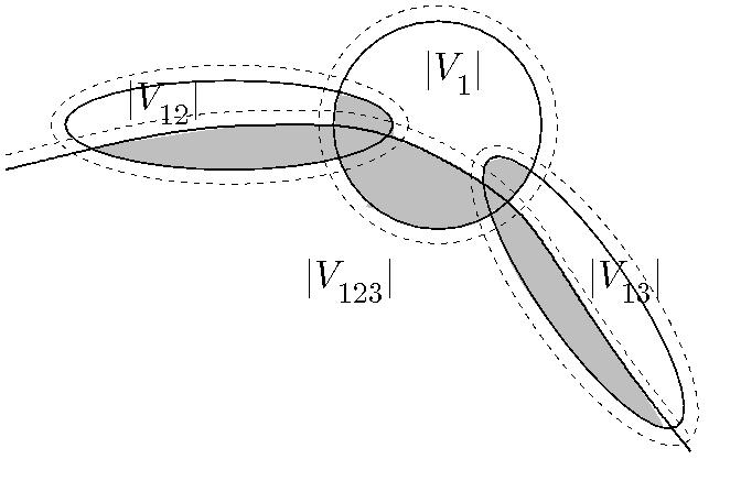
Figure 3.1. Here ${\overline{\mathcal{OL}}}(|{\mathcal{V}}|)$ is shaded, and the sets $V_{I}^{\Omega}$ are given by dotted lines; note that sets $|V_{I}^{\Omega}|$ and $|V_{J}^{\Omega}|$ are disjoint unless $I,J$ are nested.

Definition 3.1.6.

Given a subset $|W|\subset|{\mathcal{V}}^{\Omega}|$ we say that $W\subset V_{I}^{\Omega}$ is a lift of $|W|$ if

$$\pi_{\mathcal{K}}(W)=|W|,\quad W=V_{I}^{\Omega}\cap\pi_{{\mathcal{K}}}^{-1}(|W|),$$

i.e. $W$ is a ‘full’ inverse image of $|W|$ in ${\mathcal{V}}_{I}^{\Omega}$.

Lemma 3.1.7.

If $({\mathcal{U}},{\underline{{\varepsilon}}})$ is compatible, and ${\mathcal{V}}\sqsubset{\mathcal{V}}^{\Omega}\sqsubset{\mathcal{U}}$ is any nested reduction, denote by

(3.1.8) $${\overline{\mathcal{OL}}}(|{\mathcal{V}}|):={\textstyle\bigcup_{I\subsetneq K}}|\overline{V}_{IK}|\;\subset\;|{\mathcal{V}}^{\Omega}|,$$

the closure of the set of overlaps in $|{\mathcal{V}}|$. Then we may cover ${\overline{\mathcal{OL}}}(|{\mathcal{V}}|)$ by a finite number of sets $(|W_{\alpha}|)_{1\leq{\alpha}\leq N}$, where for each ${\alpha}$ there is ${\widetilde{W}}_{IK,z_{\alpha}}$ as in (3.1.6) such that

$$W_{\alpha}:={\widetilde{V}}_{IK}^{\Omega}\cap\pi_{\mathcal{K}}^{-1}(|W_{\alpha}|)\;\subset\;{\widetilde{W}}_{IK,z_{\alpha}}$$

is a lift of $|W_{\alpha}|$. Moreover, we require that $I$ is minimal and $K$ is maximal in the sense that

1. $W_{\alpha}$ is an open subset of ${\widetilde{V}}_{IK}^{\Omega}$,

2. $|V_{H}|\cap|W_{{\alpha}}|\neq\emptyset\Longrightarrow I\subset H\subset K$.

In this situation, we say that ${\mathcal{V}}$ is adapted to the cover $(|W_{\alpha}|)_{1\leq{\alpha}\leq N}$.

Proof.

Choose compatible shrinkings ${\mathcal{V}}\sqsubset{\mathcal{V}}^{1}\sqsubset\cdots\sqsubset{\mathcal{V}}^{\kappa}\sqsubset{\mathcal{V}}^{\Omega}\sqsubset{\mathcal{U}}$. Work by downwards induction on $|I|=\ell\leq{\kappa}-1$ so that at the $\ell$th stage we have a covering $(|W^{\ell}_{\alpha}|)_{{\alpha}\in B_{\ell}}$ of

$${\textstyle\bigcup_{I\subsetneq K,\ell\leq|I|}}\;|V_{IK}|$$

with lifts $W_{\alpha}^{\ell}$ satisfying (i) and such that (ii) holds if $|H|\geq\ell$. When $\ell={\kappa}-1$, the existence of the finite covering holds by the precompactness of $|{\mathcal{V}}|$ in $|{\mathcal{U}}|$ while (ii) is easy to arrange because the sets $|V_{H}|$ with $|H|=\ell$ are disjoint. Now let us suppose that this holds for $\ell+1$ with the sets $(|W_{\alpha}^{\ell+1}|)_{{\alpha}\in B_{\ell+1}}$ and consider the statement for $\ell$.

The covering $(|W_{\alpha}^{\ell}|)$ will consist of sets of two kinds:

• If $|W_{\alpha}^{\ell+1}|$ lifts to $W_{\alpha}^{\ell+1}\subset V_{I}^{{\Omega}}$ where $|I|\geq\ell+1$ is as in (i) then we take the set $|W_{\alpha}^{\prime}|$ where

  $$W_{\alpha}^{\prime}:=W_{\alpha}^{\ell+1}{\smallsetminus}{\textstyle\bigcup_{|H|=\ell}}\,{cl}({\widetilde{V}}_{HI}^{\ell}).$$

  This is open in $V_{I}^{{\Omega}}$ since we have removed a closed set, and satisfies (ii) for $\ell$. These sets cover

  $$\bigl{(}{\textstyle\bigcup_{I\subsetneq K,\ell+1\leq|I|}}\;|V_{IK}^{\ell}|\bigr{)}\;{\smallsetminus}\;\bigl{(}{\textstyle\bigcup_{H\subsetneq K,|H|=\ell}}\;{cl}(|V_{HK}^{\ell}|)\bigr{)}.$$

• Next add a finite cover of the compact set ${\textstyle\bigcup_{H\subsetneq K,|H|=\ell}}\;{cl}(|V_{HK}^{\ell}|)$ by sets $|W_{\alpha}|$ whose lifts lie in $V_{HK}^{\Omega}$ where $|H|=\ell$. These obviously satisfy (ii).

This completes the proof. ∎

Remark 3.1.8.

(i) If ${\mathcal{V}}$ is adapted to the cover $(|W_{\alpha}|)_{1\leq{\alpha}\leq N}$, and ${\mathcal{V}}^{\prime}\sqsubset{\mathcal{V}}$ is any shrinking, then ${\mathcal{V}}^{\prime}$ is also adapted to the cover $(|W_{\alpha}|)_{1\leq{\alpha}\leq N}$.

(ii) If $I\subsetneq H$ then in general ${\widetilde{V}}_{IH}$ is not closed in $V_{H}$. Therefore, in order to cover ${\overline{\mathcal{OL}}}(|{\mathcal{V}}|)$ by sets $|W_{\alpha}|$ that satisfy condition (ii) in Lemma 3.1.7 one cannot insist that each set $|W_{\alpha}|$ lift to an open subset of some $V_{I}$, but rather as in Lemma 3.1.7 (i) that it have a lift to an open subset of some $V_{I}^{\Omega}\sqsupset V_{I}$. ${\Diamond}$

Definition 3.1.9.

Suppose that $\psi^{-1}{\mathcal{G}}^{0}\sqsubset{\mathcal{V}}^{\Omega}\sqsubset{\mathcal{U}}$ where ${\mathcal{G}}^{0}\sqsubset{\mathcal{F}}$ is a reduction of the footprint cover (i.e. $G^{0}_{I}\sqsubset F_{I},\,\forall I$ and $\bigcup_{I}G^{0}_{I}=X$), and choose a shrinking ${\mathcal{V}}^{\infty}\sqsubset{\mathcal{V}}^{\omega}$ that is adapted to the cover $(|W_{\alpha}|)_{1\leq{\alpha}\leq N}$ where $|W_{\alpha}|\subset|{\mathcal{V}}^{\Omega}|$. With these choices fixed, we then say that the pair $({\mathcal{V}},{\underline{{\varepsilon}}})$ is precompatible if the following conditions hold.

1. $0<{\kappa}{\varepsilon}_{I}<{\varepsilon}_{J}$ for all $I\subsetneq J$,

2. $\psi^{-1}({\mathcal{G}}^{0})\sqsubset{\mathcal{V}}\sqsubset{\mathcal{V}}^{\infty}$;

3. $s_{I}(\overline{V_{I}})\subset E_{I,{\varepsilon}_{I}}$ for all $I$;

4. for all ${\alpha}$ with $W_{\alpha}\subset{\widetilde{V}}_{IK}^{\Omega}$ and $I\subsetneq H\subset K$

   (3.1.9) $$\phi^{E}_{IH,{\alpha}}\bigl{(}E_{H{\smallsetminus}I,({\kappa}+1){\varepsilon}_{I}}\times({\widetilde{V}}_{IH}\cap\rho_{HK}(W_{{\alpha}}\cap{\widetilde{V}}_{HK})\bigr{)}\subset V_{H}.$$

Further, we say that $({\mathcal{V}},{\underline{{\varepsilon}}})$ is compatible if it is precompatible and if $({\mathcal{V}},\,{\underline{{\varepsilon}}})\sqsubset({\mathcal{V}}^{\prime},\,{\underline{{\varepsilon}}}^{\prime})$ where $({\mathcal{V}}^{\prime},\,{\underline{{\varepsilon}}}^{\prime})$ is also precompatible and ${\underline{{\varepsilon}}}\leq{\underline{{\varepsilon}}}^{\prime}$, i.e. ${\varepsilon}_{J}\leq{\varepsilon}_{J}^{\prime}$ for all $J\in{\mathcal{I}}_{\mathcal{K}}$.

Remark 3.1.10.

If $({\mathcal{V}},{\underline{{\varepsilon}}})$ is compatible, so that it is a shrinking of the precompatible $({\mathcal{V}}^{\prime},\,{\underline{{\varepsilon}}}^{\prime})$, then we may assume that each set $|W_{\alpha}|$ of the associated covering of $|{\mathcal{V}}|$ lifts to some subset ${\widetilde{V}}_{IK}^{\prime}$. In other words, we can equivalently define $({\mathcal{V}},{\underline{{\varepsilon}}})$ to be compatible if $({\mathcal{V}},{\underline{{\varepsilon}}})\sqsubset{\mathcal{V}}^{\infty}$ is precompatible as above, for some reduction ${\mathcal{V}}^{\infty}$ that is provided with constants ${\underline{{\varepsilon}}}^{\infty}\geq{\underline{{\varepsilon}}}$ such that (a^′) and (c^′) hold. ${\Diamond}$

The next lemma shows that the hypothesis in Proposition 2.1.4 can be satisfied.

Lemma 3.1.11.

Suppose given $\psi^{-1}({\mathcal{G}}_{0})\sqsubset\psi^{-1}({\mathcal{F}}_{0})\sqsubset{\mathcal{V}}^{\infty}\sqsubset{\mathcal{V}}^{\Omega}$ such that ${\mathcal{V}}^{\infty}$ is adapted to the covering $(|W_{\alpha}|)_{1\leq{\alpha}\leq N}$, where $|W_{\alpha}|\subset|{\mathcal{V}}^{\Omega}|$. Then:

1. There is a precompatible shrinking $({\mathcal{V}},\,{\underline{{\varepsilon}}})\sqsubset{\mathcal{V}}^{\infty}$.

2. Any precompatible $({\mathcal{V}}^{\prime},\,{\underline{{\varepsilon}}}^{\prime})$ has a compatible shrinking $({\mathcal{V}},\,{\underline{{\varepsilon}}})\sqsubset({\mathcal{V}}^{\prime},\,{\underline{{\varepsilon}}}^{\prime})$.

Proof.

The proof of (i) is somewhat similar to that of Lemmas 3.1.2 and 3.1.7, except that now we have to make sure that (d^′) holds, i.e. that we can choose ${\mathcal{V}}$ so that the image of $\phi^{E}_{IH,{\alpha}}$ lies in $V_{H}$ for all $I\subsetneq H\subset K$ rather than just in the fixed ambient space $U_{J}^{\Omega}$ as in (3.1.3). Claim (ii) then follows by the same argument, with ${\mathcal{V}}^{\infty}$ replaced by ${\mathcal{V}}^{\prime}$.

To prove (i), we first choose any reduction ${\mathcal{V}}^{\kappa}$ of ${\mathcal{U}}$, where $({\mathcal{U}},{\underline{{\varepsilon}}}^{\kappa})$ is compatible, so that $({\mathcal{V}},\,{\underline{{\varepsilon}}})$ satisfies (a^′),(b^′),(c^′). We then work by downwards induction on $\ell:=|J|$, so that after the $\ell$th stage we have chosen a reduction $({\mathcal{V}}^{\ell},\,{\underline{{\varepsilon}}}^{\ell})$ with

$$\psi^{-1}({\mathcal{G}}^{0})\sqsubset{\mathcal{V}}^{\ell}\sqsubset{\mathcal{V}}^{\kappa},\quad{\underline{{\varepsilon}}}^{\ell}\leq{\underline{{\varepsilon}}}^{\kappa}$$

that satisfies (a^′), (b^′), (c^′) for all $I,K$, and satisfies (d^′) for all $I$ with $|I|\geq\ell$. Since (d^′) is vacuous when $\ell={\kappa}$, it suffices to suppose that we have found suitable $({\mathcal{V}}^{\ell+1},\,{\underline{{\varepsilon}}}^{\ell+1})$ for some $1<\ell+1\leq{\kappa}$, and consider the construction of $({\mathcal{V}}^{\ell},\,{\underline{{\varepsilon}}}^{\ell})$. Our method gives ${\underline{{\varepsilon}}}^{\ell}$ where ${\varepsilon}_{J}^{\ell}={\varepsilon}_{J}^{\ell+1}$ if $|J|>\ell$ and ${\varepsilon}_{I}^{\ell}\leq{\varepsilon}_{I}^{\ell+1}$ if $|I|\leq\ell$. Further, for $|J|>\ell$ we construct $V_{J}^{\ell}$ by removing some points in ${\widetilde{V}}_{IJ}^{\ell+1}$ from $V_{J}^{\ell+1}$ for $|I|=\ell$. Note that removing these points does not affect the validity of (d^′) for pairs $I\subsetneq K$ with $|I|\geq\ell+1$.

Choose an intermediate reduction ${\mathcal{V}}^{\prime}$ such that ${\mathcal{V}}^{0}\sqsubset{\mathcal{V}}^{\prime}\sqsubset{\mathcal{V}}^{\ell+1}$. Because the subsets $\pi_{\mathcal{K}}(V_{I}^{\infty})\subset|{\mathcal{K}}|$ with $|I|=\ell$ are disjoint, we may work separately with each such $I$. Given $x\in V_{I}$ with $I\subsetneq K=I_{\max}(|x|)$ the set ${\widetilde{V}}_{IK}^{\prime}=V_{K}^{\prime}\cap\pi_{\mathcal{K}}^{-1}(\pi_{\mathcal{K}}(V_{I}^{\prime}))$ is precompact in ${\widetilde{V}}_{IK}^{\ell+1}=V_{K}^{\ell+1}\cap\pi_{\mathcal{K}}^{-1}(\pi_{\mathcal{K}}(V_{I}^{\ell+1}))$ and hence there is $0<{\varepsilon}_{I}^{\ell}\leq{\varepsilon}_{I}^{\ell+1}$ so that for each ${\alpha}$ with $W_{\alpha}\subset V^{\Omega}_{I}$ and each $I\subsetneq H\subset K$ we have

(3.1.10) $$\phi^{E}_{IJ}\Bigl{(}E_{H{\smallsetminus}I,({\kappa}+1){\varepsilon}_{I}}\times({\widetilde{V}}_{IH}^{\prime}\cap\rho_{IH}^{-1}(W_{\alpha}))\Bigr{)}\subset V^{\ell+1}_{H}.$$

For $J$ with $|J|>\ell$ we now define

$$V_{J}^{\ell}:=V_{J}^{\ell+1}{\smallsetminus}{\textstyle\bigcup_{I\subset J,|I|=\ell}\bigl{(}s_{J}^{-1}(E_{I})\cap(V_{J}^{\ell+1}{\smallsetminus}V_{J}^{\prime})\bigr{)}}.$$

Then $V_{J}^{\ell}$ is an open subset of $V_{J}^{\ell+1}$, since we have removed a closed subset. Now choose ${\varepsilon}_{J}^{\ell}$ for $|J|<\ell$ so as to satisfy (a^′) and then define

$$V_{J}^{\ell}:=\bigl{\{}x\in V_{J}^{\ell+1}\ |\ s_{H}(x)<\tfrac{1}{2}{\varepsilon}_{J}^{\ell}\bigr{\}},\quad|J|\leq\ell.$$

Then (c^′) holds, and (b^′) still holds for $J$ with $|J|>\ell$ because it holds for ${\mathcal{V}}^{\prime}$, and it holds when $|J|\leq\ell$ because we did not change the zero sets $s_{J}^{-1}(0)$. Moreover (d^′) holds because when $|J|>\ell$ the only points in $V_{J}^{\ell+1}$ that were removed to form $V_{J}^{\ell}$ lie in $s_{J}^{-1}(E_{I})$ for $I=\ell$. But this does not affect the validity of (3.1.10) (and hence (3.1.9)) because

$$\phi^{E}_{IJ}\bigl{(}(E_{J{\smallsetminus}I,({\kappa}+1){\varepsilon}_{I}}{\smallsetminus}\{0\})\times\{z\}\bigr{)}\cap s_{J}^{-1}(E_{I})=\emptyset$$

by the first equation in (3.1.2). This completes the proof. ∎

3.2. Construction of the boundary collar

It remains to establish the existence of a collar with the properties stated in Proposition 2.1.4. Recall from (2.1.13) that ${\Delta}_{J}$ has a collar of the following form

(3.2.1) $$c_{J}^{\Delta}:{\partial}{\Delta}_{J}\times[0,{\delta}]\to{\Delta}_{J},\quad(t^{\partial},r)\mapsto(1-r|J|)\,t^{\partial}+r|J|\,b_{J},$$

where $b_{J}$ is the barycenter of ${\Delta}_{J}$ and $0<{\delta}<\frac{1}{4}$: see Figure 3.2. It is convenient to write

$${\mathcal{N}}_{\delta}^{\Delta}({\partial}_{J{\smallsetminus}I}{\Delta}):=\{t\in{\Delta}_{J}\ \big{|}\ t_{j}<{\delta},\ \forall j\in J{\smallsetminus}I\}.$$

Notice that

(3.2.2) $$c_{J}^{\Delta}\Bigl{(}({\partial}{\Delta}\cap{\mathcal{N}}_{\delta}^{\Delta}({\partial}_{J{\smallsetminus}I}{\Delta}))\times[0,{\delta})\Bigr{)}\subset{\mathcal{N}}_{2{\delta}}({\partial}_{J{\smallsetminus}I}{\Delta});$$

i.e. the width-${\delta}$ collar of the corner ${\partial}{\Delta}\cap{\mathcal{N}}_{\delta}^{\Delta}({\partial}_{J{\smallsetminus}I}{\Delta})$ lies in ${\mathcal{N}}_{2{\delta}}^{\Delta}({\partial}_{J{\smallsetminus}I}{\Delta})$. We now show that for each $J$ this collar lifts to a (partial) collar for ${\partial}Y_{{\mathcal{V}},J\,{\underline{{\varepsilon}}}}$ with the properties stated in Proposition 2.1.4.

Lemma 3.2.1.

Suppose that $({\mathcal{V}},\,{\underline{{\varepsilon}}})$ is a compatible reduction. Then for each $J\in{\mathcal{I}}_{\mathcal{K}}$ there is a constant $w_{J}>0$, subset ${\partial}^{\prime}\,Y_{{\mathcal{V}},J,\,{\underline{{\varepsilon}}}}\subset{\partial}Y_{{\mathcal{V}},J,\,{\underline{{\varepsilon}}}}$ and map $c^{Y}_{J}$ as in (2.1.22) with the properties detailed in Proposition 2.1.4.

Proof.

The proof has three steps.

Step I: Construction of local collars. As in Remark 3.1.10 we will assume that $({\mathcal{V}},{\underline{{\varepsilon}}})\sqsubset({\mathcal{V}}^{\infty},{\underline{{\varepsilon}}}^{\infty})$ is precompatible, where each set $|W_{\alpha}|$ lifts to some ${\widetilde{V}}_{IK}^{\infty}$. In this step, we fix ${\alpha},I=I_{\alpha},$ and $K=K_{\alpha}$, and define a local collar of width $w_{\alpha}$ over a subset ${\mathcal{O}}^{\infty}_{K,{\alpha}}$ of ${\partial}Y_{{\mathcal{V}}^{\infty},K,{\underline{{\varepsilon}}}^{\infty}}$. This subset is determined by the set $W_{\alpha}\subset{\widetilde{V}}_{IK}^{\infty}$, and is the inverse image of an open subset $|{\mathcal{O}}^{\infty}_{K,{\alpha}}|$ of the set of overlaps ${\overline{\mathcal{OL}}}(|{\mathcal{V}}^{\infty}|)$ in (3.1.8).

To this end, consider the coordinate chart for $Y_{{\mathcal{V}}^{\infty},K,\,{\underline{{\varepsilon}}}^{\infty}}$ given much as in (3.1.4) by

(3.2.3) $$\psi:\;E_{A{\smallsetminus}I,({\kappa}+1){\varepsilon}_{I}}\times W_{\alpha}\times[0,{\delta}_{\alpha}]^{|K{\smallsetminus}I|}\;\longrightarrow\;Y_{{\mathcal{V}}^{\infty},K,\,{\underline{{\varepsilon}}}^{\infty}},$$

$$\;\bigl{(}e_{A{\smallsetminus}I},x,r_{K{\smallsetminus}I}\bigr{)}\longmapsto\bigl{(}e_{A{\smallsetminus}I}+({\lambda}b_{I})^{-1}\cdot s_{I}(x^{\prime}),\ x^{\prime};\ {\lambda}b_{I}+r_{K{\smallsetminus}I}\bigr{)},\;\;\mbox{ where }$$

$$\;\hskip 36.135ptx^{\prime}=\phi_{IK,z_{\alpha}}^{E}(r_{K{\smallsetminus}I}\cdot e_{K{\smallsetminus}I},x),\;\;{\lambda}:=1-|r_{K{\smallsetminus}I}|=:1-{\textstyle\sum_{j\in K{\smallsetminus}I}r_{j}}.$$

For each $x\in W_{\alpha}:=W_{\alpha}\cap{\widetilde{V}}_{IK}^{\infty}$, restrict to those $r^{\partial}_{K{\smallsetminus}I}$ such that

$${\lambda}^{\partial}b_{I}+r^{\partial}_{K{\smallsetminus}I}\in\overline{\rm st}^{\Delta}_{K}(|x|)\subset{\partial}{\Delta}_{K},$$

where the superscript ${\partial}$ indicates that the corresponding point lies in the boundary. The above map provides coordinates

(3.2.4) $${\mathcal{C}}^{\delta}:\bigl{(}e_{A{\smallsetminus}I},x,r^{\partial}_{K{\smallsetminus}I}\bigr{)}\mapsto\psi\bigl{(}e_{A{\smallsetminus}I},x,r^{\partial}_{K{\smallsetminus}I}\bigr{)}=(e_{A{\smallsetminus}I}+e_{I}^{\prime\prime},x^{\prime\prime};t^{\partial})$$

for an open subset

(3.2.5) $${\mathcal{O}}_{K,{\alpha}}^{\infty}\subset\bigl{\{}(e,x;t^{\partial}):t^{\partial}\in\overline{\rm st}^{\Delta}_{K}(|x|),\ t^{\partial}\approx 0\bigr{\}}$$

of the boundary ${\partial}Y_{{\mathcal{V}}^{\infty},K,\,{\underline{{\varepsilon}}}}$. We will assume, as we may, that ${\mathcal{O}}_{K,{\alpha}}^{\infty}={\rm pr}_{V}^{-1}(|{\mathcal{O}}_{K,{\alpha}}^{\infty}|)$, where $|{\mathcal{O}}_{K,{\alpha}}^{\infty}|$ is open in ${\overline{\mathcal{OL}}}(|{\mathcal{V}}^{\infty}|)\subset|{\mathcal{V}}|$.

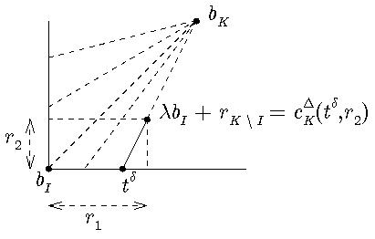
Figure 3.2. Here $K=I\cup\{1,2\}$ and $t^{\delta}$ lies on the boundary with $t_{2}=0$. Hence $r_{K{\smallsetminus}I}=(r_{1},r_{2})$ where $r_{2}$ is the collar coordinate along the ray from $t^{\delta}$ to $b_{K}$, while $t^{\delta}=c^{\Delta}_{K}(b_{I},r)$ for $r=(t^{\delta})_{1}$.

We now define a collar over ${\mathcal{O}}_{K,{\alpha}}^{\infty}$ of width $w_{\alpha}<\frac{1}{2}{\delta}_{\alpha}$ (see (3.2.2)) as follows. Given

$$(t^{\partial},r)\in\overline{\rm st}^{\Delta}_{K}(|x|)\times[0,{\delta}),\;\mbox{ where }\;(t^{\partial},r)\approx(b_{I},0),$$

choose $r_{K{\smallsetminus}I}^{\partial},r_{K{\smallsetminus}I}$ (both $\approx 0$) so that

(3.2.6) $$t^{\partial}:={\lambda}^{\partial}b_{I}+r_{K{\smallsetminus}I}^{\partial},\quad c^{\Delta}_{K}(t^{\partial},r)={\lambda}\,b_{I}+r_{K{\smallsetminus}I},\;\;$$

where ${\lambda}^{\partial}:=1-|r^{\partial}_{K-1}|,\;{\lambda}:=1-|r_{K-1}|$; see Figure 3.2. Then, with ${\mathcal{C}}^{\delta}$ as in (3.2.4), define

(3.2.7) $$c^{Y}_{K,{\alpha}}\;:\;\;{\mathcal{O}}^{\infty}_{K,{\alpha}}\times[0,w_{\alpha})\to Y_{{\mathcal{V}}^{\infty},K,\,{\underline{{\varepsilon}}}},$$

$$\bigl{(}(e_{A{\smallsetminus}I}+e_{I}^{\prime\prime},x^{\prime\prime};t^{\partial}),r\bigr{)}\stackrel{{\scriptstyle({\mathcal{C}}^{\delta})^{-1}\times{\rm id}}}{{\mapsto}}\bigl{(}\,(e_{A{\smallsetminus}I},x,r_{K{\smallsetminus}I}^{\partial}),\,r\bigr{)}\;\mapsto\;\psi\bigl{(}e_{A{\smallsetminus}I},x,r_{K{\smallsetminus}I}\bigr{)},$$

where $r_{K{\smallsetminus}I}\in[0,{\delta})^{K{\smallsetminus}I}$ is the function of $r_{K{\smallsetminus}I}^{\delta}$ and ${\delta}$ defined in (3.2.6). In particular, if $|K{\smallsetminus}I|=1$ then $r_{K{\smallsetminus}I}$ has only one component, and so is the same as the collar variable $r$, while $t^{\delta}=b_{I}$. Therefore the collar is simply given by $\psi$:

(3.2.8) $$c^{Y}_{I\cup\{j\},{\alpha}}\;:\;\;{\mathcal{O}}^{\infty}_{I\cup\{j\},{\alpha}}\times[0,w_{\alpha})\to Y_{{\mathcal{V}}^{\infty},I\cup\{j\},\,{\underline{{\varepsilon}}}},$$

$$\bigl{(}(e_{A{\smallsetminus}I}+e_{I},x;b_{I}),r\bigr{)}\mapsto\;\psi\bigl{(}e_{A{\smallsetminus}I},x,r\bigr{)}.$$

The next task is to extend the domain of this collar to

(3.2.9) $$\overline{\rm st}\bigl{(}{\mathcal{O}}^{\infty}_{K,{\alpha}}\bigr{)}:=\bigl{\{}(\mu_{H}\cdot(e,x;t)\ |(e,x;t)\in{\mathcal{O}}_{\alpha},\;\mu_{H}\cdot t\in\overline{\rm st}^{\Delta}_{K}(|x|)\bigr{\}}$$

by rescaling as follows. Consider a tuple $\mu_{H}$ (as in (2.1.28)),where $I\subset H\subsetneq K$, and point $t^{\delta}\in\overline{\rm st}^{\Delta}_{K}(|x|)\cap(\{b_{I}\}\times[0,{\delta}]^{|K{\smallsetminus}I|})$ such that

$$\mu_{H}\cdot t^{\partial}\in\overline{\rm st}^{\Delta}_{K}(|x|)\cap(\{b_{I}\}\times[0,{\delta}]^{|K{\smallsetminus}I|}),$$

and let $\mu^{\prime}_{H}\cdot$ with $(\mu_{H}^{\prime})_{i}=1$ for $i\notin H$ give the corresponding rescaling in the coordinates ${\Delta}_{I}\times[0,{\delta}_{\alpha}]^{|K{\smallsetminus}I|}$. Thus if $c^{\Delta}(t^{\partial},r)=(1-|r_{K{\smallsetminus}I}|)\,b_{I}+r_{K{\smallsetminus}I}$ as in (3.2.6), we have

(3.2.10) $$c^{\Delta}_{K}(\mu_{H}\cdot t^{\partial},r)=\mu_{H}^{\prime}\cdot({\lambda}\,b_{I}+r_{K{\smallsetminus}I}).$$

Note that this rescaling in the boundary ${\partial}_{K{\smallsetminus}H}{\Delta}_{K}$ does not affect the collar variable $r$ along this part of the boundary. Then the following diagram commutes, where we write $e_{I}^{\prime}=(t_{I})^{-1}\cdot s_{I}(x^{\prime})$, $y:=(e_{I},x;\,t_{I})\in{\partial}Y$:

(3.2.15)

because the rescaling on the left does not affect the image point $x^{\prime}=\phi(r_{K{\smallsetminus}I}\cdot e_{K{\smallsetminus}I},x)\in V_{K}$ on the right. Therefore, because $c^{Y}_{K,{\alpha}}$ is a composite of $\psi^{-1}$ (at $r=0$) with $\psi$, and because rescaling does not affect the collar variable $r$, the following diagram commutes:

(3.2.20)

In other words, if we apply the collar and then rescale (a little) by $\mu_{H}$, we get the same result as rescaling by $\mu_{H}$ and then applying the collar. It follows that we can unambiguously extend the domain of the local collar to $\overline{\rm st}({\mathcal{O}}^{\infty}_{K,{\alpha}})$ by defining

$$c^{Y}_{K,{\alpha}}\bigl{(}(e_{A{\smallsetminus}I}+e_{I}^{\prime\prime},x^{\prime\prime};\,t),r\bigr{)}:=\mu_{H}^{-1}\cdot c^{Y}_{K,{\alpha}}\bigr{(}\mu_{H}\cdot(e^{\prime},x^{\prime},t^{\prime})\bigr{)},$$

where $\mu_{H}$ is chosen so that $\mu_{H}\cdot(e^{\prime},x^{\prime},t^{\prime})$ lies in the domain of the map in (3.2.7). Note that $c^{Y}_{K,{\alpha}}$ is equivariant because the maps in (3.1.6) and (3.2.3) used to construct it are equivariant.

Although we assumed in the above construction that $K$ was maximal, so that $W_{\alpha}\subset V_{IK}^{\infty}$ this condition was not used in any essential way in the above construction. Thus for any $J$ such that $I\subsetneq J\subset K$, by using the map in (3.1.7) instead of (3.1.6) we can define a collar $c^{Y}_{J,{\alpha}}$ over

(3.2.21) $$c^{Y}_{J,{\alpha}}:\, \overline{\rm st}({\mathcal{O}}^{\infty}_{J,{\alpha}})\times[0,w_{\alpha})\to Y_{{\mathcal{V}}^{\infty},J,\,{\underline{{\varepsilon}}}^{\infty}}\;\;\mbox{ where }$$

$$\overline{\rm st}({\mathcal{O}}^{\infty}_{J,{\alpha}}): =\bigl{\{}(e,\rho_{JK}(x),t^{\partial})\in{\partial}Y_{{\mathcal{V}}^{\infty},J,{\underline{{\varepsilon}}}^{\infty}}\ \big{|}\ x\in{\widetilde{V}}_{JK}\cap W_{\alpha},(e,x;t^{\partial})\in\overline{\rm st}({\mathcal{O}}^{\infty}_{K,{\alpha}})\bigr{\}},$$

and $\overline{\rm st}({\mathcal{O}}^{\infty}_{K,{\alpha}})$ is defined in (3.2.9).

Further we can restrict these collars to the corresponding subsets $\overline{\rm st}({\mathcal{O}}_{J,{\alpha}})$ of ${\partial}Y_{{\mathcal{V}},J,\,{\underline{{\varepsilon}}}}$ for all $I\subsetneq J\subset K$, obtaining a set of locally defined collars of width $w_{\alpha}$. Note that this collar still has width $w_{\alpha}$ because we used the constant ${\varepsilon}_{I}$ in (3.2.3) rather than ${\varepsilon}_{I}^{\infty}$. Hence although ${\underline{{\varepsilon}}}<{\underline{{\varepsilon}}}^{\infty}$ in general, when we restrict the domain of $\phi$ in (3.2.3) to the points in ${\partial}Y_{{\mathcal{V}},K,\,{\underline{{\varepsilon}}}}$ the image of $\phi$ lies in $Y_{{\mathcal{V}},K,\,{\underline{{\varepsilon}}}}$ by condition (d^′) in Definition 3.1.9.

We claim that these collars satisfy all the conditions in Proposition 2.1.4. In particular, if $I\subsetneq H\subsetneq K$ the domain of $c^{Y}_{K,{\alpha}}$ contains the image of the collar $c^{Y}_{H,{\alpha}}$ by (3.2.5). They are compatible with projections and invariant under rescaling by construction.

The domains $\overline{\rm st}({\mathcal{O}}_{J,{\alpha}})$ of these collars are not open in ${\partial}Y_{{\mathcal{V}},J,\,{\underline{{\varepsilon}}}}$ because of the restriction $t\in\overline{\rm st}^{\Delta}_{J}(|x|)$, and because the condition that $(e,x;t^{\partial})\in\overline{\rm st}({\mathcal{O}}_{K,{\alpha}})$ places certain extra (but unimportant) restrictions on $\|{\rm pr}_{E_{K{\smallsetminus}I}}e\|$ when $t^{\partial}$ has been rescaled far from $b_{I}$. However, modulo these provisos, for each such $J$ they consist of the full inverse image in ${\partial}Y_{{\mathcal{V}},J,\,{\underline{{\varepsilon}}}}$ of the following open subset $|{\mathcal{O}}_{\alpha}|:=|{\mathcal{O}}_{K,{\alpha}}^{\infty}|$ of the ‘boundary’ ${\partial}|V^{\infty}_{K}|$ of $|V^{\infty}_{K}|$:

(3.2.22) $$|{\mathcal{O}}_{\alpha}|:=|{\mathcal{O}}_{K,{\alpha}}^{\infty}|\;\subset\;{\partial}|V^{\infty}_{K}|:={\textstyle\bigcup_{H\subsetneq K}}|V^{\infty}_{HK}|\subset{\overline{\mathcal{OL}}}(|{\mathcal{V}}^{\infty}|),$$

where ${\mathcal{O}}_{K,{\alpha}}^{\infty}$ is defined in (3.2.5).

Step 2: Construction of a global collar from a covering by local collars

We now explain a method from [Hat, Prop. 3.42] that combines local collars

$$\bigl{(}c_{\alpha}:{\mathcal{U}}_{\alpha}\times[0,w_{\alpha})\to Y\bigr{)}_{1\leq{\alpha}\leq N}\vspace{.07in}$$

defined over open subsets ${\mathcal{U}}_{\alpha}\subset{\partial}Y$ of the boundary of a manifold $Y$ into a global collar over ${\partial}^{\prime}\,Y$ of width $w$, where ${\partial}^{\prime}\,Y$ is any precompact subset of $\bigcup_{\alpha}{\mathcal{U}}_{\alpha}$ and $w<\min_{\alpha}w_{\alpha}/2$.

To this end, choose a partition of unity $({\lambda}_{\alpha})_{\alpha}$ subordinate to the covering of ${\partial}^{\prime}\,Y$ by the sets $(U_{\alpha})_{\alpha}$, and define

$$Y^{\prime}:=Y\cup_{\theta}\bigl{(}{\partial}^{\prime}\,Y\times[-w,0]\bigr{)},$$

where $\theta$ identifies ${\partial}^{\prime}\,Y\times\{0\}$ with ${\partial}^{\prime}\,Y$ in the obvious way. We claim that there is a homeomorphism

$$\Psi:\bigl{(}Y^{\prime},{\partial}^{\prime}\,Y\times[-w,0]\bigr{)}\longrightarrow\Bigl{(}Y,\;{\textstyle\bigcup_{{\alpha}}}c_{\alpha}\bigl{(}{\mathcal{U}}_{\alpha}\times[0,2w)\bigr{)}\Bigr{)}.$$

Granted this, we define the collar by

$$c^{Y}:{\partial}^{\prime}\,Y\times[0,w)\longrightarrow Y,\quad\bigl{(}y,r\bigr{)}\mapsto\Psi_{J}\bigl{(}\,y,\,r-w\bigr{)}.$$

The homeomorphism $\Psi$ is a composite

$$\Psi=\Psi_{N}\circ\cdots\circ\Psi_{1},$$

of homeomorphisms,

$$\Psi_{\ell}:Y^{\prime}(-1+\sum_{{\alpha}<\ell}{\lambda}_{\alpha})\to Y^{\prime}(-1+\sum_{{\alpha}\leq\ell}{\lambda}_{\alpha}),$$

where for any function ${\sigma}:{\partial}^{\prime}\,Y\to[0,1]$ we define

$$Y^{\prime}(-1+{\sigma}):=Y\cup_{\theta}\big{\{}(y,r)\ \big{|}\ y\in{\partial}^{\prime}\,Y,\ (-1+{\sigma}(y))w\leq r\leq 0\bigr{\}}.$$

To define $\Psi_{\ell}$, first extend the product structure of the external collar ${\partial}Y\times[-w,0]$ via the local collar $c_{\ell}$ to obtain an extended collar neighborhood

$$\widehat{c}_{\ell}:{\mathcal{U}}_{\ell}\times[-w,w_{\ell})\to Y^{\prime}.$$

Then define

$$\Psi_{\ell}(\widehat{c}_{\ell}(y,r)) =\widehat{c}_{\ell}(y,f_{y,\ell}(r))$$

where

$${\textstyle f_{y,\ell}:\bigl{[}(-1+\sum_{{\alpha}<\ell}{\lambda}_{\alpha}(y))w,\ 2w\bigr{]}\to\bigl{[}(-1+\sum_{{\alpha}\leq\ell}{\lambda}_{\alpha}(y))w,2w\bigr{]}}$$

is a homeomorphism that translates by ${\lambda}_{\ell}(y)$ if $r\leq\sum_{{\alpha}<\ell}{\lambda}_{\alpha}(y))w$. This completes the construction.

Remark 3.2.2.

Notice that if each local collar $c_{\alpha}$ lifts a map ${\rm pr}_{\Delta}:(Y,{\partial}Y)\to\bigl{(}[0,1),\{0\}\bigr{)}$, then the global collar does as well; i.e. we have

$${\rm pr}_{\Delta}\circ c(y,r)=r.$$

This holds because each $f_{y,\ell}$ is a translation by ${\lambda}_{\ell}(y)w$ on the relevant part of its domain, where $\sum_{\ell}{\lambda}_{\ell}(y)=1$. Further, if for some map ${\rm pr}_{E}:Y\to E$ we have $c_{\alpha}(y,r)={\rm pr}_{E}(y)$, then the global collar also satisfies $c^{Y}(y,r)={\rm pr}_{E}(y)$. ${\Diamond}$

Step 3: Completion of the proof.

Once the cover and partition of unity are chosen, the construction in Step 2 depends only on the ordering of the sets in the cover. Even though we saw in Step 1 that the local covers satisfy all the compatibility conditions required in Proposition 2.1.4, we will have to organize the construction rather carefully in order to achieve this for the global collars.

Recall from the discussion of (1.2.7) that because the atlas ${\mathcal{K}}$ is assumed tame and preshrunk and hence good, the subspace topology on $|{\mathcal{V}}^{\infty}|$ (considered as a subset of $|{\mathcal{K}}|$) is metrizable, and so we may fix a metric on $|{\mathcal{V}}^{\infty}|$. Since the sets $|V_{I}|,|V_{J}|$ have disjoint closures unless $I\subset J$ or $J\subset I$, we may choose

(3.2.23) $${\delta}_{0}>0\mbox{ smaller than half the distance between any two such sets.}$$

We next order the sets $|W_{\alpha}|_{1\leq{\alpha}\leq N}$ of the cover of ${\overline{\mathcal{OL}}}({\mathcal{V}})$ so that as ${\alpha}$ increases the cardinality $|I_{\alpha}|$ of the minimal set $I$ in Lemma 3.1.7 (i) increases. Thus we assume that there are numbers $0=n_{0}\leq n_{1}\leq n_{2}\leq\dots\leq n_{{\kappa}-1}=N$ so that

$$N_{k-1}<{\alpha}\leq N_{k}\Longrightarrow|I_{\alpha}|=k.$$

By (3.2.22) the sets $\bigl{(}|{\mathcal{O}}_{\alpha}|\bigr{)}_{1\leq{\alpha}\leq N}$ cover a neighborhood of the compact subset ${\overline{\mathcal{OL}}}(|{\mathcal{V}}|)$ in $|{\mathcal{V}}^{\infty}|$. Further by condition (ii) in Lemma 3.1.7 and our choice of $N_{k}$, if ${\alpha}>N_{k}$ the set $|{\mathcal{O}}_{\alpha}|$ does not meet any $|V_{I}|$ with $|I|\leq k$. Hence we may choose ${\delta}_{0}>{\delta}_{1}>0$ so that for each $k$, the sets $\bigl{(}|{\mathcal{O}}_{\alpha}|\bigr{)}_{1\leq{\alpha}\leq N_{k}}$ cover the closed ${\delta}_{1}$-neighborhood

$$\overline{{\mathcal{N}}}\!_{{\delta}_{1}}(k):=\overline{{\mathcal{N}}}\!_{{\delta}_{1}}\bigl{(}{\textstyle\bigcup_{|I|\leq k,L\in{\mathcal{I}}_{\mathcal{K}}}}|\overline{V_{IL}}|\bigr{)}\subset{\overline{\mathcal{OL}}}(|{\mathcal{V}}|)$$

of the compact subset ${\textstyle\bigcup_{|I|\leq k,L\in{\mathcal{I}}_{\mathcal{K}}}}|\overline{V_{IK}}|$. By shrinking the sets ${\mathcal{O}}_{\alpha}$ to ${\mathcal{O}}_{\alpha}^{\prime}$, we may then assume in addition that for some $0<{\delta}_{2}<{\delta}_{1}$ we have

(3.2.24) $$\bigl{(}{\alpha}>N_{k}\bigr{)}\,\Longrightarrow|{\mathcal{O}}_{\alpha}^{\prime}|\cap\overline{{\mathcal{N}}}\!_{{\delta}_{2}}(k)=\emptyset,\quad\forall k.$$

For each $k\leq{\kappa}$, choose a partition of unity $({\lambda}^{k}_{\alpha})_{1\leq{\alpha}\leq N_{k}}$ for $\overline{{\mathcal{N}}}\!_{{\delta}_{2}}(k)$ with respect to the covering by $(|{\mathcal{O}}_{\alpha}^{\prime}|)_{1\leq{\alpha}\leq N_{k}}$, such that

(3.2.25) $$1\leq{\alpha}\leq N_{k-1}\Longrightarrow{\lambda}^{k}_{\alpha}={\lambda}^{k-1}_{\alpha}$$

Finally, choose $w^{\prime}>0$ such that

(3.2.26) $$2w^{\prime}<{\rm min}_{\alpha}w_{\alpha}.$$

Now define

(3.2.27) $${\partial}^{k}Y_{{\mathcal{V}},J,\,{\underline{{\varepsilon}}}}={\textstyle{\bigcup_{1\leq{\alpha}\leq N_{k}}}}\bigl{\{}(e,x;t)\ |\ (e,x;t)\in\overline{\rm st}({\mathcal{O}}^{\prime}_{J,{\alpha}})\bigr{\}},$$

where $\overline{\rm st}({\mathcal{O}}^{\prime}_{J,{\alpha}})$ is defined just as in (3.2.21) but with ${\mathcal{O}}^{\infty}_{K,{\alpha}}$ replaced by ${\mathcal{O}}^{\infty}_{K,{\alpha}}\cap\pi_{\mathcal{K}}^{-1}(|{\mathcal{O}}_{\alpha}^{\prime}|)$.

Then for each $I\subsetneq J$ with $|I|=k$, we may use the local collars $c^{Y}_{J,{\alpha}}$ together with the partition of unity on ${\partial}^{k}Y_{{\mathcal{V}},J,\,{\underline{{\varepsilon}}}}$ obtained by pulling back $({\lambda}^{k}_{\alpha})$ to construct a collar

$$c^{Y}_{J,k}:{\partial}^{k}Y_{{\mathcal{V}},J,\,{\underline{{\varepsilon}}}}\times[0,w_{J}^{\prime})\to Y_{{\mathcal{V}},J,\,{\underline{{\varepsilon}}}}$$

as in Step 2. Condition 3.2.25 implies that $c^{Y}_{J,k}$ agrees with $c^{Y}_{J,k-1}$ on their common domain of definition. Hence the collars fit together to give a well defined collar

(3.2.28) $$c^{Y}_{J}:\; {\partial}^{\prime}\,Y_{{\mathcal{V}},J,\,{\underline{{\varepsilon}}}}\times[0,w_{J}^{\prime})\to Y_{{\mathcal{V}},J,\,{\underline{{\varepsilon}}}},\;\;\mbox{ where }$$

$${\partial}^{\prime}\,Y_{{\mathcal{V}},J,\,{\underline{{\varepsilon}}}}:=\textstyle{\bigcup_{k<|J|}{\partial}^{k}Y_{{\mathcal{V}},J,\,{\underline{{\varepsilon}}}}}.$$

Note that $c^{Y}_{J}$ lifts $c^{\Delta}_{J}$ by Remark 3.2.2. Thus it does have the form required by (2.1.22).

It remains to check that that we can choose collar widths $w_{J}\leq w_{J}^{\prime}$ so that the resulting collars have all the required properties.

• The maps $c^{Y}_{J}$ are equivariant, because the local collars are, and the partition of unity is pulled back from $|{\mathcal{V}}^{\infty}|$.

• To see that the $c^{Y}_{J}$ are compatible with projection to $E_{A{\smallsetminus}\bullet}$, suppose that $I\subsetneq J$ has $|I|=k<|J|$. Then $c^{Y}_{J}$ has the properties in (2.1.24) because all the local collars do. Further the points ${\iota}_{EV}(e,x)=(b_{I}^{-1}\cdot e,x;b_{I})$ mentioned in (2.1.25) lie in ${\partial}^{k}Y_{{\mathcal{V}},J,\,{\underline{{\varepsilon}}}}$. Therefore $c^{Y}_{J}({\iota}_{EV}(e,x),r)$ is made by combining the local collars $(c^{Y}_{J,{\alpha}})_{{\alpha}\leq N_{k}}$. But we saw in Step 1 that all these local collars satisfy (2.1.25) for $E_{A{\smallsetminus}I}$. It follows that the combined collar formed in Step 2 must also satisfy (2.1.25) for $E_{A{\smallsetminus}I}$.

• Similarly, the fact that the relevant local collars that form $c^{Y}_{J}$ are invariant under rescaling as in (2.1.28) implies that $c^{Y}_{J}$ also satisfies (2.1.28).

• To prove that the pairs $(c^{Y}_{J},w_{J})$ are compatible with covering maps we need to check two things:

  • that their domains are large enough (i.e. that (2.1.26) holds for all $I\subsetneq H\subsetneq J$) and

  • that when $H\subsetneq J$ the collar $c^{Y}_{H}$ has a natural lift to $Y_{{\mathcal{V}},J,\,{\underline{{\varepsilon}}}}$.

  Claim (b) again follows because the local collars used to form $c^{Y}_{H}$ (as well as the partition of unity) can be lifted in this way. (This is just a consequence of equivariance.) Claim (a) has two parts. The first claims that if $(e,x;t)\in{\partial}^{\prime}\,Y_{{\mathcal{V}},J,\,{\underline{{\varepsilon}}}}$ has $x\in{\widetilde{V}}_{IH}\cap{\widetilde{V}}_{HJ}$ where $I\subsetneq H\subsetneq J$, then $(e,\rho_{HJ}(x);t)$ is in the domain ${\partial}^{\prime}\,Y_{{\mathcal{V}},H,\,{\underline{{\varepsilon}}}}$ of $c^{Y}_{H}$. To see this, note that ${\partial}^{\prime}\,Y_{{\mathcal{V}},J,\,{\underline{{\varepsilon}}}}$ is the union over $k$ of the sets ${\partial}^{k}\,Y_{{\mathcal{V}},J,\,{\underline{{\varepsilon}}}}$ of (3.2.27). But we have

  $${\partial}^{k}\,Y_{{\mathcal{V}},J,\,{\underline{{\varepsilon}}}}\cap\bigl{\{}(e,x;t)\ |\ x\in{\widetilde{V}}_{IH}\cap{\widetilde{V}}_{HJ}\bigr{\}} ={\partial}^{|H|}\,Y_{{\mathcal{V}},J,\,{\underline{{\varepsilon}}}}\cap\bigl{\{}(e,x;t)\ |\ x\in{\widetilde{V}}_{IH}\cap{\widetilde{V}}_{HJ}\bigr{\}},$$

  $$=\bigl{\{}(e,x;t)\ |\ (e,\rho_{HK}(x);t)\in{\partial}^{|H|}\,Y_{{\mathcal{V}},H,\,{\underline{{\varepsilon}}}}\},$$

  where the first equality holds by (3.2.24), while the second holds because the sets $\overline{\rm st}({\mathcal{O}}^{\infty}_{J,{\alpha}})$ are compatible with the covering maps $\rho_{HJ}$ by (3.2.21).

  The second part of (a) concerns the choice of suitable widths $w_{H}\leq w_{H}^{\prime}$ for all $H\in{\mathcal{I}}_{\mathcal{K}}$. Since the domains of the collars are by now fixed, we can choose each $w_{H}$ independently: its choice depends only on the domains of the collars $c_{J}^{Y}$ for $J\supsetneq H$. Notice that by the definition of the set ${\mathcal{O}}^{\infty}_{K,{\alpha}}$ in (3.2.5), it holds (with $w_{H}=\frac{1}{2}{\delta}_{\alpha}$ for example) for the original domains ${\mathcal{O}}^{\infty}_{K,{\alpha}}$ of the local collars. Moreover, because ${\delta}_{2}<{\delta}_{0}$ (where ${\delta}_{0}$ is the separation distance in (3.2.23)), this property is not affected by the shrinking from $|{\mathcal{O}}^{\infty}_{K,{\alpha}}|$ to $|{\mathcal{O}}_{\alpha}^{\prime}|$ in (3.2.24). Hence it is easy to see that one can choose suitable $w_{H}$ for the global collars.

• We must check that this collar restricts to any compatible shrinking $({\mathcal{V}}^{\prime},{\underline{{\varepsilon}}}^{\prime})\sqsubset({\mathcal{V}},{\underline{{\varepsilon}}})$. But this is immediate since the above construction depends only on the choice of coordinate charts in (3.2.3) which restrict to $({\mathcal{V}}^{\prime},{\underline{{\varepsilon}}}^{\prime})$ by the definition of compatibility, and the choice of an appropriate partition of unity that we can also restrict to ${\mathcal{V}}^{\prime}$.

• Finally we must check that if ${\mathcal{K}}$ is oriented, the collar map $c^{Y}_{J}$ preserves the natural induced orientation on its domain and range. But this is clear from its construction.

This completes the proof of Lemma 3.2.1. ∎

Corollary 3.2.3.

Any reduction ${\mathcal{V}}^{\prime}$ has a collar compatible shrinking $({\mathcal{V}},{\underline{{\varepsilon}}})$.

Proof.

By Definition 2.1.5, it suffices to construct a compatible $(V_{J},{\varepsilon}_{J})$ such that

• for all pairs $I\subsetneq J$ we have ${\varepsilon}_{I}\leq w_{J}^{2}$, where $w_{J}$ is the collar width for $V_{J}$.

Without loss of generality, let us suppose that $({\mathcal{V}}^{\prime},{\underline{{\varepsilon}}}^{\prime})$ is compatible, with collars $c^{Y}_{J}$ of widths $w_{J}^{\prime}$. As in the proof of Lemma 3.1.11 we work by downwards induction on $|J|$. Hence at the $k$th stage, we assume that we have compatible $({\mathcal{V}}^{k+1},{\underline{{\varepsilon}}}^{k+1})$ such that condition (e) holds for all $I\subsetneq J$ with $|I|\geq k+1$, and aim to construct compatible $({\mathcal{V}}^{k},{\underline{{\varepsilon}}}^{k},w_{J}^{k})$ so that (e) holds whenever $|I|\geq k.$ As before we take $(V_{J}^{k},{\varepsilon}_{J}^{k},w_{J}^{k})=(V_{J}^{k+1},{\varepsilon}_{J}^{k+1},w_{J}^{k+1})$ if $|J|\geq k+1$. The key point is this: if we shrink the set $(V_{I}^{k+1},{\varepsilon}_{I}^{k+1})$ where $|I|\leq k$ by decreasing ${\varepsilon}_{I}^{k+1}$ and hence $V_{I}^{k+1}$ (because of condition (c) in Definition 3.1.1), then this does not decrease the collar width $c^{Y}_{J,k+1}$ of any $V_{J}^{k+1}$ with $I\subsetneq J$, since this change only affects points that either lie in the boundary of $Y_{{\mathcal{V}}^{k+1},J,\,{\underline{{\varepsilon}}}^{k+1}}$ or are interior points with $I(x)=\{i|s_{i}(x)\neq 0\}\subset I$ that do not occur in ${\rm im\,}(c^{Y}_{J,k+1})$ because of its construction. Hence it makes sense to choose ${\varepsilon}_{I}^{k}\leq{\varepsilon}_{I}^{k+1}$ for the elements $|I|=k$ so that condition (e) holds at level $k$, and then shrink $V_{I}^{k+1}$ to a set $V_{I}^{k}$ that satisfies (a,b,c). As usual, this can be done independently for each $I$ at level $k$. To complete the inductive step, we then make appropriate choices for lower level $I$ as in Lemma 3.1.11 to obtain a compatible shrinking $({\mathcal{V}}^{k},{\underline{{\varepsilon}}}^{k})$ that satisfies (e) at levels $\geq k$. This completes the proof. ∎

Appendix A Rational Çech cohomology and homology

We briefly describe the properties of the (co)homology theories in [Ma] that are based on the properties of Alexander–Spanier cochains. We do not need the full generality of this theory because the space $M=|{\bf M}|_{\mathcal{H}}$ is locally compact and Hausdorff. Throughout we assume that $Y$ is locally compact and Hausdorff, with $A\subset Y$ closed and $U\subset Y$ open, and take coefficients in ${\mathbb{Q}}$. Further, we denote these theories by $\check{H}$ to distinguish them from singular (co)cohomology.

We need the following properties of the cohomology theory.

• ([Ma, Thm 3.21]) If $Y$ is a connected orientable $n$-dimensional manifold then $\check{H}^{i}(Y)=0$ unless $i=n$ in which case $\check{H}^{n}(Y)={\mathbb{Q}}$, i.e. $\check{H}^{*}$ is like rational singular cohomology with compact supports;

• ([Ma, §1.2]) If $f:A\to Y$ is proper, there is an induced map $f^{*}:\check{H}^{i}(Y)\to\check{H}^{i}(A)$;

• ([Ma, §1.3]) if $U\subset Y$ is open, there is an induced map $f_{*}:\check{H}^{i}(U)\to\check{H}^{i}(Y)$. Further, if $Y$ is as in (a), and $U$ is an open $n$-disc, then $f_{*}$ is an isomorphism.

• ([Ma, Thm 1.6]) if $A\subset Y$ is closed then there is an exact sequence

  (A.1) $$\cdots\to\check{H}^{i}(Y{\smallsetminus}A)\to\check{H}^{i}(Y)\to\check{H}^{i}(A)\stackrel{{\scriptstyle{\delta}}}{{\to}}\check{H}^{i+1}(Y{\smallsetminus}A)\to\cdots,$$

  i.e. the group $\check{H}^{i}(A)$ plays the role of the relative group ${H}^{i}(Y,Y{\smallsetminus}A)$.

The dual homology theory developed in [Ma, Ch 4] is denoted $H_{*}^{\infty}$ in [Ma, Ch 10] to emphasize that it is analogous to locally finite singular homology; we shall call it $\check{H}_{*}^{\infty}$. It follows from the universal coefficient theorem [Ma, Thm. 4.17] that

(A.2) $$\check{H}_{k}^{\infty}(X)={\rm Hom}\bigl{(}\check{H}^{k}(X);{\mathbb{Q}}\bigr{)}.$$

Further, because $Y$ is locally compact and Hausdorff, it follows from the uniqueness property for $\check{H}^{*}_{c}$ stated in [Ma, §6.7], that the dual theory $\check{H}_{k}^{\infty}$ is isomorphic to rational Borel–Moore homology.

As shown by the following, the functorial properties of $\check{H}_{*}^{\infty}$ are different from the usual singular theory.

• If $Y$ is a connected orientable $n$-manifold, then $\check{H}^{\infty}_{i}(Y)=0$ unless $i=n$ in which case $\check{H}_{n}^{\infty}(Y)={\mathbb{Q}}$; more generally, any orientable $n$-manifold has a fundamental class

  (A.3) $$\mu_{Y}\in\check{H}^{\infty}_{n}(Y).$$

• ([Ma, §4.6]) if $U\subset Y$ is open, there is an induced restriction

  (A.4) $$\rho_{Y,U}:\check{H}^{\infty}_{i}(Y)\to\check{H}^{\infty}_{i}(U);$$

  moreover for $U_{1}\subset U_{2}\subset Y$ we have $\rho_{Y,U_{1}}=\rho_{U_{2},U_{1}}\circ\rho_{Y,U_{2}}$.

• ([Ma, §4.6]) If $f:A\to Y$ is continuous and proper, then there is an induced pushforward $f_{*}:\check{H}^{\infty}_{i}(A)\to\check{H}^{\infty}_{i}(Y)$; moreover, given a proper inclusion ${\iota}:A\to Y$, there is a functorial long exact sequence

  (A.5) $$\cdots\to\check{H}^{\infty}_{i}(A)\stackrel{{\scriptstyle{\iota}_{*}}}{{\to}}\check{H}^{\infty}_{i}(Y)\stackrel{{\scriptstyle\rho_{Y,Y{\smallsetminus}A}}}{{\longrightarrow}}\check{H}^{\infty}_{i}(Y{\smallsetminus}A)\stackrel{{\scriptstyle{\partial}}}{{\to}}\check{H}^{\infty}_{i-1}(A)\to\cdots$$

• ([Ma, §4.3 (3c)]) If $f:A\to Y$ is proper and $U$ is open in $Y$, then the following diagram commutes:

• ([Ma, §4.9 (6)]) if $Y=U\cup V$ where $U,V$ are open then there is an exact Mayer–Vietoris sequence of the form:

  $$\cdots\to\check{H}^{\infty}_{i+1}(U\cap V)\to\check{H}^{\infty}_{i}(Y)\to\check{H}^{\infty}_{i}(U)\oplus\check{H}^{\infty}_{i}(V)\to\check{H}^{\infty}_{i}(U\cap V)\to\cdots$$

  In particular, if $U$ is the disjoint union of a finite number of sets of $U_{i}$, then

  $$\check{H}^{\infty}_{*}(U)\cong\oplus_{i}\check{H}^{\infty}_{*}(U_{i}).$$

• ([Ma, p.334]) if $U\subset Y$ is open while $A\subset Y$ is closed, there is a cap product

  (A.6) $$\cap:\check{H}^{\infty}_{p+q}(Y{\smallsetminus}A)\otimes\check{H}^{p}(Y{\smallsetminus}U)\to\check{H}^{c}_{q}(Y,U\cup A).$$

  This takes values in compactly supported Çech homology, a theory whose functorial properties are analogous to those of the usual singular homology. In particular, if the triple $(U\cup A;U,A)$ is excisive for $\check{H}^{c}$ (i.e. $\check{H}^{c}_{q}(A,U\cap A)\cong\check{H}^{c}_{q}(U\cup A,U)$), then there is a commutative diagram

  (A.11)

  Note that the above diagram exists when $Y$ is locally compact, $A$ is closed and $Y{\smallsetminus}U$ is compact. To see this, choose a nested sequence ${\mathcal{N}}_{k}$ of precompact open neighborhoods of $Y{\smallsetminus}U$ in $Y$ with

  $$Y{\smallsetminus}U={\textstyle\bigcap_{k}}{\mathcal{N}}_{k},\quad U={\textstyle\bigcup_{k}}(Y{\smallsetminus}{\mathcal{N}}_{k}).$$

  Since by definition

  $$\check{H}^{c}_{*}(Y,U\cup A)=\underset{{\leftarrow}}{\lim}\;\check{H}^{c}_{*}(Y,(Y{\smallsetminus}{\mathcal{N}}_{k})\cup A),\qquad\check{H}^{c}_{*}(A,U\cap A)=\underset{{\leftarrow}}{\lim}\;\check{H}^{c}_{*}(A,A{\smallsetminus}{\mathcal{N}}_{k}),$$

  and the triple of closed sets $(Y,Y{\smallsetminus}{\mathcal{N}}_{k},A)$ is excisive by [Ma, Cor.9.5], it follows that $(Y,Y{\smallsetminus}U,A)$ is excisive as required.

• (Exercise 5 on p 272 of [Ma]) If $X$ is Hausdorff and $X{\smallsetminus}A$ is a precompact open subset of $X$, then $\check{H}^{\infty}_{*}(X{\smallsetminus}A)=\check{H}^{c}_{*}(X,A)$.

• This homology is taut; i.e. if $X\subset Y$ is closed, where $Y$ is locally compact and Hausdorff, and $N_{k+1}\subset N_{k}$ is a nested sequence of closed neighborhoods of $X$ in $Y$, then (by [Ma, Thm 6.4])

  $$\check{H}_{d}^{\infty}(X)=\underset{\leftarrow}{\lim}(\check{H}^{\infty}_{d}(N_{k})).$$

Acknowledgements: I thank Mohammed Abouzaid, Helmut Hofer, and Katrin Wehrheim for enlightening conversations, and Eleny Ionel and Brett Parker for very helpful comments on an earlier version of this paper. I also warmly thank the referee for a very careful reading and many pertinent comments that helped to improve the exposition and the accuracy of some of the lemmas. Finally, I thank the IAS Women and Mathematics program and the Newton Institute for Mathematical Sciences for their hospitality during the writing of this paper.

References

- [C1] R. Castellano, Smoothness of Kuranishi atlases on Gromov–Witten moduli spaces, arXiv:1511.04350.
- [C2] R. Castellano, Genus zero Gromov-Witten axioms via Kuranishi atlases, arXiv:1601.04048.
- [FF] M. Farajzadeh-Tehrani and K. Fukaya, Gromov–Witten theory via Kuranishi Structures, arXiv:1701.07821.
- [FO] K. Fukaya and K. Ono, Arnold conjecture and Gromov–Witten invariants, Topology 38 (1999), 933–1048.
- [Hat] A. Hatcher, Algebraic Topology, Wiley
- [H] H. Hofer, Polyfolds and Fredholm theory, arXiv:1412.4255, to appear in Lectures on Geometry, Clay Lecture Note series, OUP, 2017.
- [HWZ1] H. Hofer, K. Wysocki, and E. Zehnder, Applications of Polyfold theory I: The Polyfolds of Gromov–Witten theory, arXiv:1107.2097.
- [HWZ2] H. Hofer, K. Wysocki, and E. Zehnder, Polyfold and Fredholm theory, arXiv:1707.08941.
- [Ma] W. Massey, Homology and Cohomology theory, Dekker, 1978.
- [M1] D. McDuff, Branched manifolds, groupoids, and multisections, Journal of Symplectic Geometry 4 (2007) 259–315.
- [M2] D. McDuff, Notes on Kuranishi atlases, arXiv:1411.4306
- [M3] D. McDuff, Strict orbifold atlases and weighted branched manifolds, to appear in J. Symp. Geom., arXiv:1506.05350
- [MW1] D. McDuff and K. Wehrheim, The topology of Kuranishi atlases, Proceedings of the London Mathematical Society (3) 115 (2017), no 2, 221-292.
- [MW2] D. McDuff and K. Wehrheim, The fundamental class of smooth Kuranishi atlases with trivial isotropy, Journal of Topology and Analysis Vol 10 (2018).
- [MW3] D. McDuff and K. Wehrheim, Smooth Kuranishi atlases Geometry & Topology 21-5 (2017), 2725–2809.
- [MW4] D. McDuff and K. Wehrheim, work in progress.
- [P] John Pardon, An algebraic approach to virtual fundamental cycles on moduli spaces of -holomorphic curves, Geom. Topol. 20 (2016), 779-1034.
- [Y] Dingyu Yang, The polyfold–Kuranishi correspondence I: a choice-independent theory of Kuranishi structures, arXiv:1402.7008