Thermoelectric efficiency of nanoscale devices in the linear regime

Abstract

We study quantum transport through two-terminal nanoscale devices in contact with two particle reservoirs at different temperatures and chemical potentials. We discuss the general expressions controlling the electric charge current, heat currents and the efficiency of energy transmutation in steady conditions in the linear regime. With focus in the parameter domain where the electron system acts as a power-generator, we elaborate workable expressions for optimal efficiency and thermoelectric parameters of nanoscale devices. The general concepts are set at work in the paradigmatic cases of Lorentzian resonances and antiresonances, and the encompassing Fano transmission function: the treatments are fully analytic, in terms of the trigamma functions and Bernoulli numbers. From the general curves here reported describing transport through the above model transmission functions, useful guidelines for optimal efficiency and thermopower can be inferred for engineering nanoscale devices in energy regions where they show similar transmission functions.

I INTRODUCTION

Thermoelectricity is an old and young subject of enormous interest both for the fundamental physical phenomena involved DRESS12 ; ZLATIC14 and the technological applications.SALVO99

At the birth of research of thermoelectric (TE) materials, Seebeck demonstrated that it is possible to convert waste heat into electricity, while Peltier showed that refrigeration of a TE material can be obtained pumping heat by means of electricity. After almost two centuries, it is still a central problem to find the conditions to realize a most efficient Carnot machine for a given finite power output WHIT14 also in conditions of large temperature and electrical potential gradients.MUTTALIB13

The energy conversion efficiency of a TE material is measured by the figure of merit dimensionless number defined as $ZT=\sigma S^{2}T/(\kappa_{el}+\kappa_{ph})$, where $\sigma$ is the electronic conductance, $S$ the Seebeck coefficient, $T$ the absolute temperature and $\kappa_{el}$ ($\kappa_{ph}$) is the electronic (phononic) contribution to the thermal conductance.

The promise of a TE material with highest figure of merit is a challenge for theoretical and experimental research. DRESS12 At first sight the way to maximize $ZT$ for a given material could seem to increase the quantity $\sigma S^{2}$, for instance enhancing the charge carriers density by doping, or reducing the contributions to its thermal conductance. However, increasing $\sigma$ (or $S$) without increasing $\kappa_{el}$, is a conflicting task and still remains the goal: in fact room temperature values of $ZT$ for the best bulk TE materials are around unity, in a range of values not yet satisfactory for large-scale applications.

An alternative approach SOFO96 was suggested by Mahan and Sofo in 1996. Starting from a given phononic thermal conductivity of a TE material, and the expression of the transport coefficients given by the Boltzmann equation, they looked for the electronic structure which generates an energy dependent transport distribution function able to maximize the figure of merit. Their mathematical approach led to conclude that a delta-shaped transport distribution function maximize the transport properties. Successive contributions FAN11 ; JEONG12 addressing the effect of more realistic band structure and transmission shapes evidenced that finite band-widths (e.g. of rectangular shape) produce higher thermoelectric performances and this occurs both in the linear CHANG14 and nonlinear WHIT14 regime.

The concept of engineering of the electronic band structure to enhance the figure of merit received great impulse from progress in nanotechnology DRESS07 and advances in the synthesis of complex SNYDER08 and organic materials.KATZ12 Modulation of the electronic properties of nano- and of organic molecular-electronic materials have opened perspectives for the control and enhancement of $ZT$, mainly due to confinement effects and the possibility they offer to reduce the phononic thermal conductivity.YU10 ; LI14 In particular, the prediction BERG09 ; BERG10 of giant thermoelectric effects on conjugated single molecule junctions characterized by nodes and supernodes in the transmission spectrum contributed to increase the interest toward organic thermoelectrics.

In the present paper we focus on a general two-terminal nanoscale device in contact with two particle reservoirs, the left and right ones, at different temperatures and chemical potentials: $T_{L},\mu_{L}$ and $T_{R},\mu_{R}$. The general expressions provided by the Keldysh formalism DATTA ; GOOD09 ; CUEVAS10 ; BALZER13 ; CRESTI06 are the most appropriate to evaluate the transmission function, that controls quantum transport of charge and heat through the system at the atomistic level. Here we adopt the linear regime for the difference of the Fermi functions of the left and right reservoirs, $f(E,\mu_{L},T_{L})-f(E,\mu_{R},T_{R})$; moreover, for sake of simplicity, we consider pure electronic transport. In the particular case that many-body effects (such as electron-electron, electron-phonon or phonon-phonon interactions NICOLIC12 ) are made negligible, the Landauer approach is recovered DATTA03 ; JEONG10 . Anyhow, if many body interactions are present in the central device, the Keldysh formalism can anyway encompass at the appropriate level of approximation wide classes of many-body scattering processes, and we here mention just as an example the successful proposal of electron-phonon interaction in the lowest order approximation FRED05 ; FRED014 ; FRED16 ; CUEVAS05 , and other possible analytic simplifications.BEVI16

The key ingredient for the description of transport in the spirit of the Keldysh formalism and mean field approach, is the electronic transmission function ${\mathcal{T}}(E)$ which contains the microscopic physics of the sample under temperature and chemical potential differences, and its connection with the leads. Numerous first-principle calculations have been proposed based on density functional theory in the Green’s function many-body formalism to study electronic and thermal conductances in nanoscale and molecular systems SANVITO06 ; NIKO12 ; TAKAI16 ; MINGO06 ; WANG08 , often combined with tight binding Hamiltonians.NICOLIC12 ; DATTA03

To pick-up the essentials of charge and electronic thermal contribution to coherent transport in TE, in this paper we do not go through ab initio evaluation of the transmission function, but we focus on special functional shapes, such as Fano transmission functions and Lorentzian resonances and antiresonances, most frequently encountered in the actual transmission profiles of nanostructured systems, due to quantum interference effects. In particular, the review by Lambert LAMB15 on quantum interference effects in single-molecule electronic transport has underlined the importance of recognizing the peak and dip nature in the evaluated landscape of ${\mathcal{T}}(E)$ and how they can be tuned by appropriate system parameters, as recently implemented also by stretching.TORRES15 ; TSUT15 For instance, in a molecular system coupled to electrodes, Breit-Wigner (Lorentzian)-like BW36 transmission function occurs at electron energies which approach the energies of the composing orbitals for sufficiently spaced molecular levels. On the other side, the ubiquitous asymmetric Fano like resonances FANO61 ; MIRO10 ; Huang15 ; SSP may occur e.g. in chains of molecular systems with attached groups when the energy of the electron resonates with a bound state of the pendant group CHAKRA06 ; FARCHION12 .

Impact of Breit-Wigner and Fano transmission shapes on the TE properties of nanostructured materials have been recognized for graphene quantum rings ORELLANA15 and nanoribbons NICOLIC12 ; GONG13 but also for quantum dots SANCHEZ15 ; ORELLANA12 , and in the vast field of molecular electronics CUEVAS10 ; FARC96 for nanoscale molecular bridges and molecular wires,LAMB14 ; SUAREZ13 ; LAMB09 ; MURPHY08 ; LAMB06 and molecular constrictions. Noticeably, molecular junctions have been proposed MURPHY08 as optimal candidates for large values of the figure of merit $ZT$.

Our paper aims to a systematic study of paradigmatic model nanosystems, because of their own interest and in order to infer guidelines for optimal efficiency and thermopower of actual TE quantum structures. To keep the presentation reasonably self-contained, in Section II we summarize relevant aspects of quantum transport for molecular devices, in the linear response regime. In Section III we elaborate the transport parameters with some significant rationalization. In particular a novel expression of the efficiency of the device is worked out. Convenient expressions of electric conductance, thermopower coefficient, thermal conductance, power output, Lorenz function, performance parameter and efficiency are reported in terms of kinetic parameters defined in dimensionless form. In Section IV and in Section V the general concepts are specified in the case of the Fano transmission function and the encompassed Lorentzian resonances and antiresonances; it is remarkable and rewarding that the treatment becomes fully analytic, in terms of polygamma functions and Bernoulli numbers. This permits deeper physical insight on the variegated aspects of carrier transport and the instructive numerical simulations reported in Section VI. By virtue of our procedure, analytic in a wide extent and fully analytic in a number of significant limits in the parameter domain, universal features describing transport in Fano-like models emerge with great evidence. This is of major interest on its own right; also, and more importantly, the universal curves may provide useful guidelines for realistic nanosystems, whose transmission lineshapes can be tailored and fitted with the studied models in some appropriate energy ranges. Section VII contains the conclusions.

II Transport equations in the linear response regime for molecular devices

The transport equations of a nanoscale system of non-interacting electrons are essentially controlled by the transmission function ${\mathcal{T}}(E)$. The charge (electric) current $I_{e}$, the left and the right heat (thermal) currents $I_{Q}^{(left)}$ and $I_{Q}^{(right)}$, the input or output power ${\mathcal{P}}$ (with ${\mathcal{P}}>0$ in power-generators, and ${\mathcal{P}}<0$ in refrigerators), the efficiency $\eta$ (in power generation) and the efficiency $\eta_{refr}$ (in refrigeration) due to the transport of (spinless) electrons across a mesoscopic device in stationary conditions are given by the expressions GOOD09 ; CUEVAS10

$$I_{e}=I_{e}^{(left)}=I_{e}^{(right)}=\frac{-e}{h}\int_{-\infty}^{+\infty}dE\,{\mathcal{T}}(E)\left[f_{L}(E)-f_{R}(E)\right]$$ (1a)

$$I_{Q}^{(left)}=\frac{1}{h}\int_{-\infty}^{+\infty}dE(E-\mu_{L})\,{\mathcal{T}}(E)\left[f_{L}(E)-f_{R}(E)\right]$$ (1b)

$$I_{Q}^{(right)}=\frac{1}{h}\int_{-\infty}^{+\infty}dE(E-\mu_{R})\,{\mathcal{T}}(E)\left[f_{L}(E)-f_{R}(E)\right]$$ (1c)

$${\mathcal{P}}=I_{Q}^{(left)}-I_{Q}^{(right)}=\frac{1}{h}\,(\mu_{R}-\mu_{L})\int dE\,{\mathcal{T}}(E)\left[f_{L}(E)-f_{R}(E)\right]$$ (1d)

$$\eta=\frac{I_{Q}^{(left)}-I_{Q}^{(right)}}{I_{Q}^{(left)}}=(\mu_{R}-\mu_{L})\frac{\int dE\,{\mathcal{T}}(E)\left[f_{L}(E)-f_{R}(E)\right]}{\int dE(E-\mu_{L})\,{\mathcal{T}}(E)\left[f_{L}(E)-f_{R}(E)\right]}$$ (1e)

$$\eta_{refr}=\frac{I_{Q}^{(right)}}{I_{Q}^{(left)}-I_{Q}^{(right)}}=\frac{\int dE(E-\mu_{R})\,{\mathcal{T}}(E)\left[f_{L}(E)-f_{R}(E)\right]}{\int dE(\mu_{R}-\mu_{L})\,{\mathcal{T}}(E)\left[f_{L}(E)-f_{R}(E)\right]}$$ (1f)

where $e=|e|$ is the absolute value of the electronic charge. The positive direction in the one-dimensional device has been chosen from the left reservoir to the central device in the left lead, and from the central device to the right reservoir in the right lead. Notice that Eqs.(1) hold in the linear and non-linear regime, and apply to thermal devices, regardless if they act as output-power generators or input-power absorbers (i.e. refrigerators, often addressed as heat pumps).

We are here interested in the linear response of the system and assume that $\Delta\mu=\mu_{L}-\mu_{R}$ and $\Delta T=T_{L}-T_{R}$ can be treated as infinitesimal quantities. For power generators, the appropriate operative conditions can be specified as follows:

(i) Without loss of generality, from now on, it is assumed that the left reservoir is the hot one and the right reservoir is the cold one, namely:

$$\Delta T=T_{L}-T_{R}>0\ .$$ (2a)

The quantity $$\Delta T \Delta\mu$$ is always positive (regardless if finite or infinitesimal); on the contrary, the sign of the quantity is controlled or chosen case-by-case.

(ii) The power generators mimic in principle a macroscopic thermal machine if heat is extracted from the hot reservoir and a fraction of it is transmitted to the cold reservoir. This entails that both the left heat current and the right heat currents are positive, and the former is larger than the latter; namely:

$$I_{Q}^{(left)}>I_{Q}^{(right)}>0.$$ (2b)

The difference of the left and right thermal currents represents the output power of the nanoscale thermal generator. In Fig.1 we report schematically the picture of transport through nanoscale power generator.

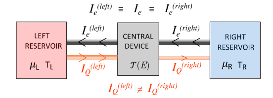
Figure 1: Schematic representation of a two-terminal power-generator device, with electron transmission function ${\mathcal{T}}(E)$, and $T_{L}>T_{R}$. In steady situation, the charge current is conserved in the left and right electrodes. Heat current is not conserved, and heat flowing from the hot source is partially transmitted to the cold one. [For refrigerators, maintaining $T_{L}>T_{R}$, the arrows must be oriented in the opposite direction].

The situation of refrigerators could be dealt with in a similar way: in the cooling mode the nanoscale device satisfies the conditions

$$I_{Q}^{(left)}<I_{Q}^{(right)}<0\ ,$$ (2c)

with heat flowing from the cool reservoir to the hot one; the difference of the left and right thermal currents represents the power absorbed from the nanoscale thermal refrigerator. In this work we consider explicitly only the case of power generation, since the case of power absorption is akin.

Linearization of the transport equations

Consider the Fermi distribution function

$$f(E;\mu,T)=\frac{1}{e^{(E-\mu)/k_{B}T}+1}\equiv f(E)\ ;$$

the derivatives with respect to the energy, the temperature and the chemical potential are linked by the relations

$$\frac{\partial f}{\partial E}=-\frac{1}{k_{B}T}\cdot\frac{e^{(E-\mu)/k_{B}T}}{[e^{(E-\mu)/k_{B}T}+1]^{2}}\quad;\quad\frac{\partial f}{\partial\mu}\equiv-\frac{\partial f}{\partial E}\quad;\quad\frac{\partial f}{\partial T}\equiv\frac{E-\mu}{T}\,(-\frac{\partial f}{\partial E})\ .$$ (3)

In the linear approximation, the Fermi function of the right reservoir can be expanded in terms of the Fermi function of the left reservoir in the form

$$f(E;\mu_{R},T_{R})=f(E;\mu_{L},T_{L})+(\mu_{R}-\mu_{L})\frac{\partial f_{L}}{\partial\mu_{L}}+(T_{R}-T_{L})\frac{\partial f_{L}}{\partial T_{L}}\ .$$

We denote by $\Delta T$ (with $\Delta T>0$) the temperature difference between the left and right reservoir, with $\Delta\mu$ the difference of the chemical potential, and with $\Delta V$ the applied bias; namely

$$\Delta T=T_{L}-T_{R}\ (>0)\ \ ,\ \ \Delta\mu=\mu_{L}-\mu_{R}\ \ ,\ \ \Delta\mu=(-e)\Delta V\ \ ,\ \ \Delta V=V_{L}-V_{R}\ .$$ (4)

It follows

$$f_{L}(E)-f_{R}(E)=(-\frac{\partial f_{L}}{\partial E})\left[\Delta\mu\ +\ (E-\mu_{L})\,\frac{\Delta T}{T_{L}}\right].$$ (5)

The transport equations (1) for charge current, heat current, power-output and the efficiency parameter become for low voltage bias and low temperature bias:

$$I_{e} = \frac{-e}{h}\int dE\,{\mathcal{T}}(E)\,(-\frac{\partial f_{L}}{\partial E})\left[-e\,\Delta V+(E-\mu_{L})\dfrac{\Delta T}{T_{L}}\right]$$ (6a)

$$I_{Q}^{(left)} = \frac{1}{h}\int dE\,(E-\mu_{L})\,{\mathcal{T}}(E)\,(-\frac{\partial f_{L}}{\partial E})\left[-e\,\Delta V+(E-\mu_{L})\frac{\Delta T}{T_{L}}\right]$$ (6b)

$${\mathcal{P}} = \frac{1}{h}\,e\,\Delta V\int dE\,{\mathcal{T}}(E)\,(-\frac{\partial f_{L}}{\partial E})\left[-e\,\Delta V+(E-\mu_{L})\frac{\Delta T}{T_{L}}\right]$$ (6c)

$$\eta = e\,\Delta V\frac{\int dE\,{\mathcal{T}}(E)\,(-\dfrac{\partial f_{L}}{\partial E})\left[-e\,\Delta V+(E-\mu_{L})\dfrac{\Delta T}{T_{L}}\right]}{\int dE\,(E-\mu_{L})\,{\mathcal{T}}(E)\,(-\dfrac{\partial f_{L}}{\partial E})\left[-e\,\Delta V+(E-\mu_{L})\dfrac{\Delta T}{T_{L}}\right]}\,.$$ (6d)

At this stage, in the conventional elaboration of the transport properties of nanoscale systems, it is customary to introduce the kinetic transport coefficients $L_{0},L_{1},L_{2}$ usually in the form

$$L_{n}=\frac{1}{h}\int dE\,{\mathcal{T}}(E)(E-\mu_{L})^{n}(-\frac{\partial f_{L}}{\partial E})\ \qquad(n=0,1,2)\ .$$

It is seen by inspection that the electric charge current and the heat current $(I_{e},I_{Q}^{(left)})$ are linked to the bias potential and bias temperature $(\Delta V,\Delta T)$ via a $2\times 2$ matrix, controlled by $L_{1,2,3}$. It is also apparent that the units of the coefficients $L_{n}$ change with $n$ and are given by $\ {\rm(eV)}^{n-1}\cdot{\rm sec^{-1}}\$.

For the purpose of this article, that focuses on performance of devices, optimization conditions, and comparison of transmission functions, it is useful (and “practically necessary”) to clearly disentangle quantities under elaboration from the entailed units of measure. For a deeper understanding of the physics of transport processes, and also for computational purposes, it is preferable and rewarding to process dimensionless quantities, adopting units based on fundamental constants or combination of fundamental constants, as shown in detail in the next section.

III Dimensionless kinetic parameters and natural units for nanoscale devices

The structure of Eqs.(6), and the previous discussed motivations, suggest to define the dimensionless kinetic transport coefficients $K_{n}$ as follows

$$K_{n}=\int dE\,{\mathcal{T}}(E)\,\frac{(E-\mu)^{n}}{(k_{B}T)^{n}}\,(-\frac{\partial f}{\partial E})=K_{n}(\mu,T)\quad(n=0,1,2)\ ,$$ (7)

where $\mu=\mu_{L}\ ,\ T=T_{L}\ {\rm and}\ f=f_{L}$. It is apparent that $K_{0}$ and $K_{2}$ are positive quantities, while $K_{1}$ can be either positive or negative; furthermore $K_{1}$ certainly vanishes whenever the transmission function is an even function with respect to the chemical potential.

The expression of the kinetic coefficients $K_{n}$ can be conveniently worked out with the Sommerfeld expansion SSP , provided the transmission function is reasonably smooth on the scale of the thermal energy $k_{B}T$ (which is the energy scale of the derivative of the Fermi function). In the treatment of nanostructures the Sommerfeld expansion is hardly applicable, and other procedures must be considered. In the paradigmatic case of Fano transmission function and alike, we show in Appendix A that the kinetic transport coefficients can be obtained analytically.

From the structure of Eq.(7), it can be noticed that the expressions $K_{0},K_{1},K_{2}$ are the zero, first and second moment of the definite positive function, given by the product the transmission function times the opposite of the derivative of the Fermi function. The moments of any definite positive function satisfy basic and general restrictions, and in particular for $K_{0,1,2}$ it holds

$$\frac{K_{2}}{K_{0}}\geq\left(\frac{K_{1}}{K_{0}}\right)^{2}\quad\Longleftrightarrow\quad K_{2}\,\geq\,\frac{K_{1}^{2}}{K_{0}}\quad\Longleftrightarrow\quad\frac{K_{1}^{2}}{K_{0}K_{2}}\leq 1\ .$$ (8)

We exploit the above inequality for defining a novel key parameter of far reaching significance

$$p=\frac{K_{1}^{2}}{K_{0}K_{2}}\qquad({\rm with}\ \ 0\leq p\leq 1)\ .$$ (9)

The so defined p-performance parameter is dimensionless and confined in the interval from zero to unity. The upper bound holds only when the energy spread of the definite positive integrand in Eq.(7) vanishes. The lower bound holds when $K_{1}=0$, and in particular whenever the transmission function is even with respect to the chemical potential.

The performance parameter $p$ characterizes and controls the efficiency of the nanoscale thermal device, as we show in detail in Appendix B. It is remarkable that the optimal efficiency $\eta$ of the device, inferred from Eq.(6d), is linked to the $p$-performance parameter by the simple expression:

$$\frac{\eta}{\eta_{c}}=\frac{1-\sqrt{1-p}}{1+\sqrt{1-p}}\ ,$$ (10)

where

$$\eta_{c}\equiv\frac{\Delta T}{T}\equiv\frac{T_{L}-T_{R}}{T_{L}}\quad(T=T_{L}>T_{R})\$$ (11)

is the efficiency of the ideal Carnot cycle. It is almost superfluous to add that the optimal efficiency of the device, provided by Eq.(10) is smaller than the Carnot cycle efficiency, as required by the general principles of thermodynamics. It is also apparent that the efficiency $\eta$ takes its maximum value $\eta_{c}$ for $p=1$, and decreases monotonically to zero for decreasing values of $p$.

We now insert into Eqs.(6) the kinetic transport parameters defined in Eqs.(7). To simplify a little bit the notations (with attention to avoid ambiguities), in Eqs.(7) the temperature $T_{L}$ and the chemical potential $\mu_{L}$ for the left reservoir are denoted dropping the subscript $L$ for left, i.e. $T_{L}\rightarrow T$ and $\mu_{L}\rightarrow\mu$; the same simplified notation is applied to Eqs.(6). Then, the transport equations (6) take the compact and significant form

$$I_{e} = \frac{e^{2}}{h}K_{0}\,\Delta V-\frac{e^{2}}{h}\frac{k_{B}T}{e}K_{1}\frac{\Delta T}{T}$$ (12a)

$$I_{Q}^{(left)} = -\frac{e^{2}}{h}\frac{k_{B}T}{e}K_{1}\,\Delta V+\frac{e^{2}}{h}\frac{k_{B}^{2}T^{2}}{e^{2}}K_{2}\frac{\Delta T}{T}$$ (12b)

$${\mathcal{P}} = -\frac{e^{2}}{h}K_{0}\,(\Delta V)^{2}+\frac{e^{2}}{h}\frac{k_{B}T}{e}K_{1}\,\Delta V\,\frac{\Delta T}{T}\ \left[\equiv I_{Q}^{(left)}-I_{Q}^{(right)}\right]$$ (12c)

$$\eta = \frac{\ \ -K_{0}\,(\Delta V)^{2}\ +\ \dfrac{k_{B}T}{e}K_{1}\,\Delta V\,\dfrac{\Delta T}{T}}{-\dfrac{k_{B}T}{e}K_{1}\,\Delta V+\dfrac{k_{B}^{2}T^{2}}{e^{2}}K_{2}\,\dfrac{\Delta T}{T}}\ \left[\equiv\frac{{\mathcal{P}}}{I_{Q}^{(left)}}\right]\ .$$ (12d)

The ingredients of Eqs.(12) involve the dimensionless kinetic parameters $K_{0,1,2}$, and the Carnot efficiency $\eta_{c}$ of an ideal device working between the temperatures $T_{L}>T_{R}$. Eqs.(12) also contain the applied bias potential $\Delta V$, and the so called “thermal potential” $\phi_{T}$, defined by the relation $\phi_{T}\equiv k_{B}T/e$. The quantum of conductance $e^{2}/h$ also appears naturally.

Using Eqs.(12), the transport coefficients of interest in measurements, such as the electric conductance, the Seebeck coefficient, the thermal conductance, the Lorenz number, the power output and the efficiency parameter, can be worked out as follows.

Consider first the thermoelectric system in isothermal situation, i.e. with the electrodes kept at the same temperature. Eq.(12a) in the absence of temperature gradients gives

$$\Delta T\equiv 0\ \ \Longrightarrow\ \ I_{e}=\frac{e^{2}}{h}K_{0}\,\Delta V\equiv\sigma_{0}\,\Delta V\quad{\rm with}\quad\ \sigma_{0}=K_{0}\,\frac{e^{2}}{h}\ .$$ (13)

The isothermal conductance $\sigma_{0}$ represents the proportionality coefficient between the electric current and the applied voltage $\Delta V$, with no temperature gradient across the sample.

In the general situation when a voltage and a temperature gradient are both applied to the thermoelectric system, the electric current given by Eq.(12a) can be written in the more effective form

$$I_{e} = \frac{e^{2}}{h}\,K_{0}\left[\Delta V-\frac{K_{1}}{K_{0}}\,\frac{k_{B}T}{e}\,\frac{\Delta T}{T}\right]$$ (14)

$$= \sigma_{0}\left[\,\Delta V+S\,\Delta T\right]\quad{\rm with}\quad S(T,\mu)=-\frac{K_{1}}{K_{0}}\,\frac{k_{B}}{e}\ ;$$

the contribution to the electric current, proportional to the temperature bias, defines the thermoelectric power or Seebeck coefficient $S$. In open circuit situation, we have $I_{e}=0$; this means that the thermoelectric power represents essentially the potential drop for unitary temperature gradient for zero electric current.

From Eq.(12a) we can extract for $\Delta V$ the expression:

$$\Delta V=\frac{1}{(e^{2}/h)K_{0}}I_{e}+\frac{K_{1}}{K_{0}}\,\frac{k_{B}T}{e}\,\frac{\Delta T}{T}\ .$$

Replacement of such a value into Eq.(12b) gives

$$I_{Q}^{(left)}=-\frac{e^{2}}{h}\,\frac{k_{B}T}{e}\,K_{1}\left[\frac{1}{(e^{2}/h)K_{0}}I_{e}+\frac{K_{1}}{K_{0}}\,\frac{k_{B}T}{e}\,\frac{\Delta T}{T}\right]+\frac{e^{2}}{h}\,\frac{k_{B}^{2}T^{2}}{e}\,K_{2}\,\frac{\Delta T}{T}\ .$$

Then

$$I_{Q}^{(left)}=-\frac{K_{1}}{K_{0}}\,\frac{k_{B}T}{e}\,I_{e}+\kappa_{el}\Delta T\qquad{\rm with}\qquad\kappa_{el}=T\,(K_{2}-\frac{K_{1}^{2}}{K_{0}})\,\frac{k_{B}^{2}}{h}\ ,$$ (15)

where $\kappa_{el}$ defines the electronic contribution to the thermal conductance of the system (heat current per unit temperature gradient for zero electric current). The ratio between the thermal conductance and the electric conductance is called the Lorenz number; it is given by

$$L=\frac{\kappa_{el}}{\sigma_{0}T}=\frac{K_{0}K_{2}-K_{1}^{2}}{K_{0}^{2}}\,\frac{k_{B}^{2}}{e^{2}}\ .$$ (16a)

Thermal conductance and Lorenz number are essentially positive quantities, as can be inferred from their physical meaning and from the inequality (8). Another parameter traditionally used in the literature is the dimensionless figure of merit. Neglecting lattice conductance, the figure of merit for electrons carrier transport reads

$$(ZT)_{el}=\frac{T\sigma_{0}S^{2}}{\kappa_{el}}=\frac{S^{2}}{L}=\frac{K_{1}^{2}}{K_{0}K_{2}-K_{1}^{2}}\ .$$ (16b)

From Eq.(9) and Eq.(16b) one can see that the $$(ZT)_{el} p$$ and parameters are linked by the relations

$$(ZT)_{el}=\frac{p}{1-p}\quad\Longrightarrow\quad p=\frac{(ZT)_{el}}{(ZT)_{el}+1}$$ (16c)

The operative conditions for molecular power-generators

The operative conditions for molecular power-generators imply a positive power-output; such requirement using Eq.(12c) reads

$${\mathcal{P}}=-\frac{e^{2}}{h}K_{0}\,(\Delta V)^{2}+\frac{e^{2}}{h}\,\frac{k_{B}T}{e}\,K_{1}\,\Delta V\,\frac{\Delta T}{T}>0\ .$$ (17)

Since $\Delta T$ and $K_{0}$ are both positive, a necessary condition to satisfy Eq.(17) is that $K_{1}$ and $\Delta V$ have the same sign. The output power vanishes for

$$\Delta V=0\quad{\rm and}\quad\Delta V=\frac{K_{1}}{K_{0}}\,\frac{k_{B}T}{e}\,\frac{\Delta T}{T}\ .$$

Suppose we have chosen the parameters $T,\mu$ for the left reservoir (the hotter of the two reservoirs), and also fix $\Delta T(>0)$. The only variable parameter in Eq.(17) remains $\Delta V$. It is apparent that

$${\rm if}\quad K_{1}>0\quad\Longrightarrow\quad{\mathcal{P}}>0 \quad{\rm for}\quad 0<\Delta V<\frac{K_{1}}{K_{0}}\,\frac{k_{B}T}{e}\,\frac{\Delta T}{T}$$ (18a)

$${\rm if}\quad K_{1}<0\quad\Longrightarrow\quad{\mathcal{P}}>0 \quad{\rm for}\quad \frac{K_{1}}{K_{0}}\,\frac{k_{B}T}{e}\,\frac{\Delta T}{T}<\Delta V<0\ .$$ (18b)

The optimized maximum value of the power-output occurs at midway of the intervals indicated in Eqs.(18), and reads

$${\mathcal{P}}=\frac{1}{4}\,\frac{K_{1}^{2}}{K_{0}}\,\frac{k_{B}^{2}T^{2}}{h}\,(\frac{\Delta T}{T})^{2}=\frac{1}{4}\frac{K_{1}^{2}}{K_{0}}\,\frac{k_{B}^{2}}{h}\,T^{2}\,\eta_{c}^{2}\ .$$ (19)

Natural units for nanoscale devices

For sake of completeness we briefly summarize the natural units encountered so far. The natural unit of conductance is given by the quantum of conductance

$$\frac{e^{2}}{h}=\frac{1}{25812.807}\,\Omega^{-1}=3.874046\cdot 10^{-5}\ \frac{\rm A}{\rm V}\ ;$$ (20a)

the value is based on the von Klitzing constant $$h/e^{2} e^{2}/h$$, whose experimental accuracy is better than eight significant digits. The conductance of a single periodic chain in the allowed energy region equals .

The natural unit of Seebeck thermoelectric power is

$$\frac{k_{B}}{e}=86.17\ \frac{\mu{\rm V}}{\rm K}\ .$$ (20b)

Good thermoelectric materials have thermoelectric powers of the order of $k_{B}/e$. Notice that the ratio between the Boltzmann constant and the electron charge can also be conveniently replaced by $\phi_{T}/T$, where $\phi_{T}=k_{B}T/e$ is the thermal voltage (a quantity and a concept embedded in the architecture of electronic circuits see Ref.SEDRA10, ).

For instance, at room temperature $T_{0}=300\ K$, $\phi_{0}\approx 0.025\$V, and $\phi_{0}/T_{0}$ recovers Eq.(20b), as expected.

For the Lorenz number (or better: for the Lorenz function) the natural unit is given by the square of Eq.(20b); namely

$$\frac{k_{B}^{2}}{e^{2}}=74.25\cdot 10^{-10}\,\frac{{\rm V}^{2}}{{\rm K}^{2}}\ .$$ (20c)

And finally for the thermal conductance a useful unit is given by the following combination of universal constants

$$\frac{k_{B}^{2}}{h}=1.8\cdot 10^{6}\ \frac{\rm eV}{\rm sec}\cdot\frac{1}{\rm K^{2}}\ ,$$ (20d)

which can be seen as the counterpart of Eq.(20a) for the electric conductance.

For convenience, the thermoelectric transport parameters, expressed in terms of dimensionless kinetic coefficients and natural units, are summarized in Table 1.

Nanostructure: ${\mathcal{T}}(E)$ transmission function
Dimensionless kinetic parameters: $K_{n}=\int dE\,{\mathcal{T}}(E)\dfrac{(E-\mu)^{n}}{(k_{B}T)^{n}}(-\dfrac{\partial f}{\partial E})$
$\sigma_{0}=K_{0}\,\dfrac{e^{2}}{h}$	$S=-\dfrac{K_{1}}{K_{0}}\,\dfrac{k_{B}}{e}$	$\dfrac{{\mathcal{P}}}{\eta_{c}^{2}}=\dfrac{1}{4}\,T^{2}\,\dfrac{K_{1}^{2}}{K_{0}}\,\dfrac{k_{B}^{2}}{h}$
$\kappa_{el}=T(K_{2}-\dfrac{K_{1}^{2}}{K_{0}})\,\dfrac{k_{B}^{2}}{h}$		$L=\dfrac{\ K_{0}K_{2}-K_{1}^{2}\ }{K_{0}^{2}}\ \dfrac{k_{B}^{2}}{e^{2}}$
$p=\dfrac{K_{1}^{2}}{K_{0}K_{2}}\quad(0\leq p\leq 1)$	$(ZT)_{el}=\dfrac{p}{1-p}$	$\dfrac{\eta}{\eta_{c}}=\dfrac{1-\sqrt{1-p}}{1+\sqrt{1-p}}$

Table 1: Transport parameters in the linear approximation for thermoelectric materials, with electronic transmission function ${\mathcal{T}}(E)$. The kinetic parameters $K_{0,1,2}$ are defined in dimensionless form. The electric conductance $\sigma_{0}$, Seebeck coefficient $S$, power-output ${\mathcal{P}}$, thermal conductance $\kappa_{el}$, Lorenz number $L$, performance parameter $p$, figure of merit $(ZT)_{el}$ and efficiency ${\eta}$ are reported. The quantity $\eta_{c}$ denotes the Carnot cycle efficiency $\eta_{c}=\Delta T/T$, where $\Delta T$ is the temperature difference between the hot reservoir and the cool one.

IV Kinetic parameters for Fano lineshapes in the linear response regime

The Fano lineshape transmission function can be written in the form

$${\mathcal{T}}_{F}(E)=\frac{(E-E_{d}+q\Gamma_{d})^{2}}{(E-E_{d})^{2}+\Gamma_{d}^{2}}\ ,$$ (21)

where $E_{d}$ is the intrinsic level of the model, $\Gamma_{d}(>0)$ is the broadening parameter, and the dimensionless parameter $q$ (supposed real and positive) is the asymmetry profile.

The dimensionless kinetic parameters corresponding to the Fano transmission function can be evaluated analytically for any range of the thermal energy. The kinetic integrals for the Fano transmission probability become

$$K_{n}=\int_{-\infty}^{+\infty}dE\,\frac{(E-E_{d}+q\Gamma_{d})^{2}/(k_{B}T)^{2}}{(E-E_{d})^{2}/(k_{B}T)^{2}+\Gamma_{d}^{2}/(k_{B}T)^{2}}\,\frac{(E-\mu)^{n}}{(k_{B}T)^{n}}\,\frac{1}{k_{B}T}\frac{e^{(E-\mu)/k_{B}T}}{[e^{(E-\mu)/k_{B}T}+1]^{2}}\ .$$

As usual, it is convenient to introduce the dimensionless variables

$$z=\frac{E-\mu}{k_{B}T}\quad;\quad dz=\frac{dE}{k_{B}T}\quad;\quad\gamma=\frac{\Gamma_{d}}{k_{B}T}\quad;\quad\varepsilon=\frac{E_{d}-\mu}{k_{B}T}$$

$$\frac{E-E_{d}}{k_{B}T}=\frac{(E-\mu)-(E_{d}-\mu)}{k_{B}T}\equiv z-\varepsilon,$$

where $\varepsilon$ and $\gamma$ are two dimensionless parameters that, together with the asymmetry parameter $q$, fully specify the Fano model under attention. The $\varepsilon$ parameter specifies the position of the intrinsic level $E_{d}$ relative to the Fermi level in units of thermal energy, while $\gamma$ specifies the broadening parameter again in units of thermal energy. The asymmetry parameter ($q\approx 1-5$ or so) is often considered as an assigned value of the model, although it is of course a third parameter itself. With the indicated substitutions, one obtains

$$K_{n}=\int_{-\infty}^{+\infty}dz\,\frac{(z-\varepsilon+q\gamma)^{2}\,z^{n}}{(z-\varepsilon)^{2}+\gamma^{2}}\,(-\frac{\partial f}{\partial z})\qquad\ {\rm with}\qquad f(z)=\frac{1}{e^{z}+1}\ .$$ (22)

Notice that for real arguments $(\varepsilon,\gamma)$ the kinetic coefficients are real functions, as expected.

For the calculation of Eq.(22), it is convenient to elaborate the denominator using the identity

$$\frac{1}{(z-\varepsilon)^{2}+\gamma^{2}}\equiv\frac{i}{2\gamma}\left[\frac{1}{z-\varepsilon+i\gamma}-\frac{1}{z-\varepsilon-i\gamma}\right]\ .$$

The kinetic functions defined in Eq.(22) can be written in the form

$$K_{n}=\frac{i}{2\gamma}\int_{-\infty}^{+\infty}\,dz\,\left[\frac{(z-\varepsilon+q\gamma)^{2}z^{n}}{z-\varepsilon+i\gamma}-\frac{(z-\varepsilon+q\gamma)^{2}z^{n}}{z-\varepsilon-i\gamma}\right]\,(-\frac{\partial f}{\partial z})\ .$$

Taking into account that the parameters $(\varepsilon,\gamma,q)$ are real quantities, we have

$$K_{n}=2\,{\rm Re}\left\{\frac{i}{2\gamma}\int_{-\infty}^{+\infty}\,dz\,\frac{(z-\varepsilon+q\gamma)^{2}z^{n}}{z-\varepsilon+i\gamma}\,(-\frac{\partial f}{\partial z})\right\}.$$

We can thus write for the kinetic parameters of the Fano lineshape the expression

$$K_{n}=\frac{1}{\gamma}\,{\rm Re}\left\{i\,\int_{-\infty}^{+\infty}dz\,\frac{\ z^{n+2}-2(\varepsilon-q\gamma)z^{n+1}+(\varepsilon-q\gamma)^{2}z^{n}\ }{z-\varepsilon+i\gamma}\,(-\frac{\partial f}{\partial z})\right\}\ .$$ (23)

In Appendix A, we show that the above integrals can be calculated analytically by means of the trigamma function, and Bernoulli numbers.

For this purpose, we resort to the the set of auxiliary complex functions defined in Eq.(A2), and here repeated

$$I_{n}(w)=i\int_{-\infty}^{+\infty}dz\,\frac{z^{n}}{z-w}\,(-\frac{\partial f}{\partial z})\qquad{\rm Im}\,w<0$$ (24)

where $w=\varepsilon-i\gamma$ is a complex variable, independent from the asymmetry parameter of the Fano lineshape. In Appendix A we show that all $I_{n}$ can be expressed in terms of $I_{0}$, and furthermore $I_{0}$ can be calculated analytically with the trigamma function $\Psi_{t}$.ABRA The kinetic parameters $K_{n}$ of Eq.(23) can be expressed in the form

$$K_{n}=\frac{1}{\gamma}\,{\rm Re}\left[I_{n+2}(w)-2(\varepsilon-q\gamma)I_{n+1}(w)+(\varepsilon-q\gamma)^{2}I_{n}(w)\right]\ ,$$ (25)

where

$$I_{0}(w)=\dfrac{1}{2\pi}\,\Psi_{t}(\dfrac{1}{2}+\dfrac{iw}{2\pi}),\qquad I_{n}(w)=ib_{n-1}+w\,I_{n-1}(w)\,\,\,\,{\rm for}\,\,\,\,n\geq 1,$$

and $b_{n}$ are the Bernoulli-like numbers:

$$b_{0}=1\ ,\ b_{1}=0\ ,\ b_{2}=\frac{\pi^{2}}{3}\ ,\ b_{3}=0\ ,\ b_{4}=\frac{7\pi^{4}}{15}\ ,\ b_{5}=0,\,\ b_{6}=\frac{31\pi^{6}}{21}\ ,\ \ldots$$

Then the thermoelectric parameters can be calculated using the expressions summarized in Table 1.

A particular case of the Fano transmission function occurs when the asymmetry parameter vanishes. The antiresonance lineshape, setting $q=0$ into Eq.(21), reads

$${\mathcal{T}}_{A}(E)=\frac{(E-E_{d})^{2}}{(E-E_{d})^{2}+\Gamma_{d}^{2}}\ .$$ (26)

The kinetic parameters for the antiresonance lineshape, setting $q=0$ into Eq.(25), and straigt algebraic elaborations become

$$K_{0} = 1-\frac{\gamma}{2\pi}{\rm Re}\,\Psi_{t}(\frac{1}{2}+\frac{iw}{2\pi}),$$ (27a)

$$K_{1} = -\frac{\gamma}{2\pi}{\rm Re}\left[w\,\Psi_{t}(\frac{1}{2}+\frac{iw}{2\pi})\right],$$ (27b)

$$K_{2} = \frac{\pi^{2}}{3}\!-\gamma^{2}-\frac{\gamma}{2\pi}{\rm Re}\left[w^{2}\,\Psi_{t}(\frac{1}{2}+\frac{iw}{2\pi})\,\right].$$ (27c)

V Kinetic parameters for Breit-Wigner (Lorentzian) lineshapes in the linear response regime

The Lorentzian-like transmission lineshape can be written in the form

$${\mathcal{T}}_{L}(E)=\frac{\Gamma_{d}^{2}}{(E-E_{d})^{2}+\Gamma_{d}^{2}}\ ,$$ (28)

where $E_{d}$ is the intrinsic resonance level of the model, and $\Gamma_{d}(>0)$ is the broadening parameter. The kinetic parameters corresponding to the Lorentzian transmission function can be evaluated analytically for any range of the thermal energy, chemical potential, location and broadening of the resonant level. The hybridization energy $\Gamma_{d}$ sets the lifetime $\tau=\hbar/\Gamma_{d}$ of the electron in the quantum system. We can consider the Lorentz transmission as the particular case of the Fano lineshape when the asymmetry parameter $q\rightarrow\infty$ (and division by $q^{2}$ is performed). From Eq.(25), that provides the kinetic parameters of the Fano lineshape, we obtain that the kinetic parameter of the Lorentzian lineshape read

$$K_{n}=\gamma\,{\rm Re}\,I_{n}(w)$$ (29)

The explicit values of $K_{0},K_{1},K_{2}$ of interest for the treatment of of thermoelectrics in the energy windows with Lorentzian transmission function are the following:

$K_{0}\!=\!\frac{\gamma}{2\pi}{\rm Re}\Psi_{t}(\frac{1}{2}+\frac{iw}{2\pi})$,    $K_{1}\!=\!\frac{\gamma}{2\pi}{\rm Re}\left[w\,\Psi_{t}(\frac{1}{2}+\frac{iw}{2\pi})\right]$,    $K_{2}\!=\!\gamma^{2}+\frac{\gamma}{2\pi}{\rm Re}\left[w^{2}\,\Psi_{t}(\frac{1}{2}+\frac{iw}{2\pi})\,\right]$.

VI Simulation of model thermoelectrics

We consider now some simulations of molecular power-generators, with particular interest to establish domain regions where the efficiency is as near as possible to unity, and the thermopower is large. We begin with the study of the Lorentzian model for the transmission function, together with the complementary case of antiresonance lineshape. Then we examine the situation of the Fano transmission function. These models, can be solved analytically with the trigamma function and Bernoulli numbers, and provide useful guidelines in the understanding and designing thermoelectric devices.

A. Transport through Lorentzian transmission functions

The transport properties through the Lorentzian transmission function are controlled by the two dimensionless parameters $(\varepsilon,\gamma)$: the energy parameter $\varepsilon=(E_{d}-\mu)/k_{B}T$ specifies the position of the electronic level of the quantum system with respect to the chemical potential in units of thermal energy; the second one $\gamma=\Gamma/k_{B}T$ specifies the lineshape broadening again in units of the thermal energy. Small values of $\gamma$ (typically $\gamma<1$) characterize long lifetime electronic states, while large values of $\gamma$ (typically $\gamma>1$) characterize short lifetime electronic states.

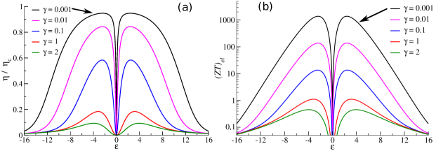
Figure 2: Universal curves for: (a) the efficiency $\eta/\eta_{c}$, and (b) the figure of merit $(ZT)_{el}$, of the thermal machine with Lorentzian lineshape as a function of the dimensionless energy parameter $\varepsilon=(E_{d}-\mu)/k_{B}T$, for fixed values of the dimensionless broadening parameter $\gamma=\Gamma/k_{B}T$. Notice the logarithmic scale on the vertical axis of panel (b).

We begin with the discussion of the behavior of the (relative) efficiency $\eta/\eta_{c}$, and we report in Fig.2a the family of universal curves for the efficiency of the thermal machine with Lorentzian lineshape transmission as a function of the dimensionless parameter $\varepsilon$, for fixed values of the broadening dimensionless parameter. The values chosen for the broadening parameter are the set of values $\gamma=2,1,0.1,0.01,0.001$; in the case of a thermal machine operating around room temperature the set corresponds to the values $\Gamma=50,25,2.5,0.25,0.025$  meV.

It can be noticed that the plots in Fig.2a are symmetric with respect to $\varepsilon$, and approach zero for vanishing $\varepsilon$ and for large $\varepsilon$; this can also be confirmed by appropriate analytic expansion of the trigamma function.

From Fig.2a it is seen that the efficiency takes its optimal values for $\varepsilon\approx 2-4$ (or so) for most values of the broadening parameter. In this range of $\varepsilon$ values, the efficiency for long-lived states $(\gamma\ll 1)$ is near unity, while for short-lived states $(\gamma\gg 1)$ the efficiency is rather poor. Thus, the good feature of near unity efficiency must be matched (and maybe to some extent conflicting) with the simultaneous requirement of rather small broadening. This unavoidable link in Lorentzian lineshapes between good efficiency and tendentially small broadening is broken by the asymmetry parameter of Fano lineshapes, and represents a major point of interest of the Fano structures, as we shall see below.

A transport property of primary interest is the Seebeck thermopower, and we examine the parameter-region where the (absolute) values of the thermopower are reasonably large, i.e. of the order of $k_{B}/e$ or so. From the curves reported in Fig.3, it emerges with evidence that long-lived quantum states ($\gamma<<1$) are the candidates for high thermopower. For molecular devices with Lorentzian lineshapes, it can be noticed that the thermoelectric power is positive when the chemical potential is larger than the resonance energy (i.e. $\mu>E_{d}\Longrightarrow\varepsilon<0$); it is zero (by virtue of the symmetry of the lineshape) at the resonance energy; it is negative when the chemical potential is smaller than the resonance energy (i.e. $\mu<E_{d}\Longrightarrow\varepsilon>0$); it goes to zero for large values of $|\varepsilon|$. In principle, the Seebeck coefficient can assume (absolute) values higher or much higher than $k_{B}/e$, provided $\gamma$ becomes extremely small. Of course, large values of Seebeck coefficients are of interest when the efficiency of the thermal machine is also advantageous, and nanostructures with the desired parameter characteristics are experimentally achievable.

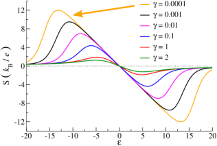
Figure 3: Universal curves for the thermoelectric power (in units $k_{B}/e$) of Lorentzian transmission functions, versus the dimensionless energy parameter $\varepsilon=(E_{d}-\mu)/k_{B}T$, for fixed values of the dimensionless broadening parameter $\gamma=\Gamma/k_{B}T$.

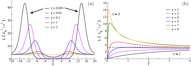
Figure 4: (a) Universal family of curves for the Lorenz number (in units $k_{B}^{2}/e^{2}$) versus the energy parameter $\varepsilon=(E_{d}-\mu)/k_{B}T$ for fixed values of $\gamma=\Gamma/k_{B}T$ of the resonance transmission function, and (b) versus the broadening parameter $\gamma$ for fixed values of $\varepsilon$. The straight line drawn at $\pi^{2}/3$ represents the common asymptotic value of the family of curves for large values of $\gamma$.

We report now in Fig.4 the results for the Lorenz number (or better the Lorenz function). It is well known that the Lorenz number approaches the asymptotic (Bernoulli-like) value of $\pi^{2}/3$ whenever the transmission function is rather smooth in the thermal energy scale $k_{B}T$ (provided no node occurs in the energy interval under attention); this can be shown with the Sommerfeld expansion, usually applicable in massive macroscopic thermoelectrics.SSP From Fig.4a, it can be seen that the family ofr curves of the Lorenz number are all depressed with respect to $\pi^{2}/3$ for $|\varepsilon|$ around the origin; then the curves attain values larger (or much larger) than $\pi^{2}/3$ for intermediate values of $|\varepsilon|$, and finally go to the Sommerfeld constant $\pi^{2}/3$ for high $|\varepsilon|$ values. This down and up behavior is particularly evident for small values of $\gamma$. These features are also corroborated by analytic investigations. From Fig.4b, it can also be noticed that the curves with $\varepsilon<4$ (or so) go from zero to the asymptotic value, in tendentially monotonic way; on the contrary, curves with higher values of $\varepsilon>4$ (or so) overcome the asymptotic value before approaching it for large $\gamma$. Thus for nanoscale devices the Lorenz number is very far from being constant, and can be both depressed or enhanced with respect to the Sommerfeld constant. The region of depression or enhancement is most interesting for the material performance, because the Wiedemann-Franz law is broken and more flexibility in tailoring thermoelectric properties becomes possible.

B. Transport through antiresonance transmission functions

We consider now transport properties through the antiresonance transmission function

$${\mathcal{T}}_{A}(E)=\frac{(E-E_{d})^{2}}{(E-E_{d})^{2}+\Gamma_{d}^{2}}\ ,$$ (30)

and compare with the results obtained in the previous subsection in the case of resonances. In Fig.5a we report the efficiency $\eta/\eta_{c}$ of antiresonance lineshapes versus the energy parameter $\varepsilon$, for fixed values of the broadening parameter $\gamma$. It is apparent that the efficiency curves are even with respect to $\varepsilon$, and go to zero for small and large $\varepsilon$; this behavior is confirmed by appropriate analytic manipulations.

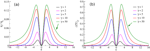
Figure 5: Universal curves for: (a) the efficiency $\eta/\eta_{c}$, and (b) the figure of merit $(ZT)_{el}$, of the thermal machine with antiresonance lineshape as a function of the energy parameter $\varepsilon=(E_{d}-\mu)/k_{B}T$, for fixed values of the broadening parameter $\gamma=\Gamma/k_{B}T$ .

From Fig.5a, it can also be seen that the optimal efficiency increases with $\gamma$ up to $\gamma\approx 50$, and then it tends to saturate (the curve with $\gamma=100$, not reported, nearly overlaps with the curve with $\gamma=50$). This behavior of the efficiency of antiresonances is in striking contrast with the case of Lorentz resonance, where the efficiency always decreases with increasing $\gamma$, as pictured in Fig.2a. Of course the optimal working conditions of any device are in practice controlled by a trade-off among different requirements, including efficiency, Seebeck coefficient, actual availability and preparation of materials in the conditions forecast as promising by the simulations.

In Fig.6 we report the Seebeck thermopower, for antiresonant levels, characterized by the $(\varepsilon,\gamma)$ parameters. The values of the thermopower are of the order of $k_{B}/e$ (or so) for $\gamma$ around unity, and saturate to $\approx 1.8\,k_{B}/e$ for larger values of $\gamma$. Differently from the behavior of the thermopower of the resonant structure of Fig.3, the Seebeck coefficient of the antiresonance increases with $\gamma$, until it saturates for $\gamma\approx 50$. It can be noticed that the thermoelectric power is zero for $\varepsilon=0$ (by virtue of the symmetry of the lineshape), and approaches zero for large $|varepsilon|$; in the region $\varepsilon<0$ the Seebeck coefficient is negative, while it is positive for $\varepsilon>0$. Thus for the antiresonant structure the Seebeck coefficient is negative for $\mu>E_{d}$ and is positive for $\mu<E_{d}$. The opposite signs occur for the resonant structure of Fig.3. The antiresonant structure produces a Seebeck coefficient with a hole-liken behavior. In essence, the comparison of the Seebeck thermopower for the Breit-Wigner resonance (Fig.3) and for the antiresonance (Fig.6) shows that, in appropriate situations, it could become preferable to engineer antiresonances, rather than insist in strong peaked structures.

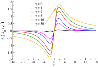
Figure 6: Universal curves of thermoelectric power (in units $k_{B}/e$) of antiresonance transmission functions, versus the energy parameter $\varepsilon=(E_{d}-\mu)/k_{B}T$, for fixed values of the broadening parameter $\gamma=\Gamma/k_{B}T$.

Fig.7 reports the Lorenz number as function of the energy parameter $\varepsilon$ for antiresonant structures. The curves reported in Fig.7 are enhanced with respect to the asymptotic value $\pi^{2}/3$ for $|\varepsilon|$ around the origin, present values somewhat smaller than $\pi^{2}/3$ for intermediate values of $|\varepsilon|$, and finally reach the Sommerfeld constant of $\pi^{2}/3$ for high values of $|\varepsilon|$. This up and down behavior is particularly evident for high values of $\gamma$. The comparison with the family of curves of Fig.4a for resonant structures, further highlights similarities and differences of resonance and antiresonance structures in the transmission function.

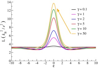
Figure 7: Universal curves for the the Lorenz number of antiresonance transmission functions, versus the energy parameter $\varepsilon=(E_{d}-\mu)/k_{B}T$, for fixed values of the broadening parameter $\gamma=\Gamma/k_{B}T$.

C. Transport through Fano transmission functions

At this stage we pass to consider the Fano-like lineshapes in the transmission function, which can present in dependence of the intrinsic asymmetry parameter $q$, either a Lorentz resonant level, or antiresonance, or any intermediate structure.

$${\mathcal{T}}_{F}(E)=\frac{(E-E_{d}+q\Gamma_{d})^{2}}{(E-E_{d})^{2}+\Gamma_{d}^{2}}\ .$$ (31)

The transport properties through the Fano transmission function are controlled by two dimensionless parameters $(\varepsilon,\gamma)$, and by the asymmetry parameter $q$ (assumed to be a positive number; for negative number the curves must be reversed); the values $q=0$ and $q=\infty$ correspond to the symmetric antiresonance and symmetric resonance Lorentzians, respectively, while intermediate values of $q$ produce asymmetric situations.

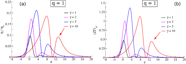
Figure 8: Universal curves for: (a) the efficiency $\eta/\eta_{c}$ and (b) the figure of merit $(ZT)_{el}$, of the thermal machine with Fano lineshape as a function of the dimensionless energy parameter $\varepsilon=(E_{d}-\mu)/k_{B}T$, for fixed values of the broadening parameter $\gamma=\Gamma/k_{B}T$. The asymmetry parameter $q$ has been set equal to 1.

We begin with the discussion of the behavior of the efficiency $\eta/\eta_{c}$, and we report in Fig.8a the family of universal curves for the efficiency of the thermal machine with Fano lineshape as a function of the dimensionless parameter $\varepsilon$, for fixed values of the broadening parameter $\gamma$; in these simulations we set the value of the $q$ parameter equal to unity. We notice that the efficiency is not symmetric with respect to $\varepsilon$, and goes to zero for large $|\varepsilon|$. A comparison of Fig.8a (corresponding to $q=1$) and Fig.5a (corresponding to $q=0$) shows that the efficiencies for $\varepsilon>0$ for Fano lineshapes are enhanced with respect to the efficiencies for $\varepsilon>0$ of the antiresonance. In the case of Fano lineshapes the asymmetry parameter adds further flexibility to the engineering of molecular thermal machines.

We pass now to the Seebeck coefficient. In Fig.9 we report the thermopower for the Fano transmission lineshape for fixed value $\gamma=1$ and $q=0,\,\pm 1,\,\pm 2$. As expected the curves with parameters $\pm q$ exhibit inversion symmetry with respect to the origin of the $\varepsilon$ variable. It is important to notice that the curves with $q=0,\,\pm 1,\,\pm 2$ (as well other values not reported) show a substantial increase of the absolute value of the Seebeck thermopower, compared with the curve $q=0$ of the antiresonant structure and already discussed in Fig.6.

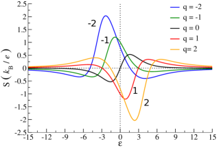
Figure 9: Thermoelectric power (in units $k_{B}/e$) for Fano transmission functions, versus the $\varepsilon=(E_{d}-\mu)/k_{B}T$ energy parameter, for different values of the asymmetry parameter $q$. The broadening parameter $\gamma=\Gamma/k_{B}T$ has been chosen equal to unity.

InFig.10, i we report the thermoelectric power of Fano transmission functions for fixed values of $\gamma$, and values $q=1$ and $q=5$ of the asymmetry parameter. From Fig.10 it is seen that the Seebeck coefficient assumes absolute values of the order of $k_{B}/e$ or more as $\gamma$ increases; the same occurs for increasing values of $q$, as it can also be confirmed by appropriate manipulations of the trigamma function. Thus from a qualitative point of view, the analysis of the Fano structure hints the possibility of good thermoelectric devices with high efficiency and Seebeck thermopower, and relatively large broadening. In summary, the link between good efficiency and small broadening of Lorentzian lineshapes is broken to some extent in antiresonances, and further relaxed for Fano-like transmission lineshapes.

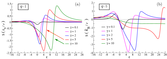
Figure 10: (a) Thermoelectric power (in units $k_{B}/e$) for Fano transmission functions, versus the energy parameter $\varepsilon=(E_{d}-\mu)/k_{B}T$, for fixed values of the broadening parameter $\gamma=\Gamma/k_{B}T$. The asymmetry parameter $q$ has been set equal to 1 in panel (a) and equal to 5 in panel (b).

VII Conclusions

This article addresses quantum transport through nanoscale thermoelectric devices, and discuss the general equations controlling the electric charge current, heat currents, and efficiency of energy transmutation in steady conditions in the linear regime. With focus in the parameter domain where the electron system acts as a molecular power-generator, we provide the expressions of optimal efficiency, electric and thermal conductance, Lorenz number and power-output of the device. The treatment is fully analytic and presented in terms of trigamma functions and Bernoulli numbers.

The general concepts are put at work in paradigmatic devices with Lorentzian resonances and anti-resonances transmission functions. A most important feature of this investigation is the emergency of the complementary roles of peaked and valleyed structures: in the former the most interesting region of application involves long-lived electron states $(\gamma\ll 1)$, while in the latter it involves $\gamma\gg 1$ structures. The simulations are then extended to the paradigmatic case of Fano transmission functions, that encompass peaked and valleyed regions. In the case of Fano lineshapes, the role of the asymmetry parameter can be exploited to widen the region of good performance of the devices, and to add further flexibility to the engineering of molecular thermal machines.

The procedures elaborated in this article can be extended to non-linear situations, as well as to systems with broken time-reversal symmetry. Within the framework of the non-equilibrium Keldysh formalism, the approach can be generalized to handle interacting quantum systems and in particular electron-phonon interactions, which have been so fruitfully explored in the lowest order approximation. In all these variegated subjects, the approaches elaborated in this work can be of help for developing protocols and in depth understanding of the non-equilibrium processes accompanying charge and heat currents, and efficiency of energy transmutation in nanoscale devices.

Appendix A. Some integrals for the analytic treatment of thermoelectricity with Fano lineshape transmission

In the treatment of thermoelectric effects in nanoscale systems with Fano or Fano-like lineshapes in the linear regime, we have to consider integrals of the type

$$I_{n}(w)=i\int_{-\infty}^{+\infty}dz\,\frac{z^{n}}{z-w}\,(-\frac{\partial f}{\partial z})\ \ (n=0,1,2,\ldots)\quad f(z)=\frac{1}{e^{z}+1}\ \ ,\ \ {\rm Im}\,w<0\ ,$$ (A1)

where $f(z)$ is the Fermi function (with unitary thermal energy and zero chemical potential), and $w$ is a complex variable located in the lower half part of the complex plane. The purpose of this Appendix is to provide an analytic expression of the $I_{n}(w)$-integrals, which are just the key ingredient for the calculation of the thermoelelctric parameters. First, we show that $I_{0}(w)$ can be calculated analytically with the trigamma function. Next, by virtue of recurrence relations, we express any $I_{n}(w)$ with $n=1,2,3,\ldots$ in terms of $I_{0}(w)$.

Analytic evaluation of $I_{0}$

The auxiliary integral $I_{0}(w)$, according to Eq.(A1), reads

$$I_{0}(w)=i\int_{-\infty}^{+\infty}dz\,\frac{1}{z-w}\,(-\frac{\partial f}{\partial z})\quad,\quad{\rm Im}\,w<0\quad,\quad f(z)=\frac{1}{e^{z}+1}\ .$$ (A2)

For the analytic evaluation of $I_{0}$ we exploit the multipole series expansion of the derivative of the Fermi distribution function.

The Fermi-Dirac distribution function can be expanded in the series

$$f(z)=\frac{1}{e^{z}+1}\equiv\frac{1}{2}-\sum_{n=-\infty}^{+\infty}\,\frac{1}{\,z-(n+1/2)2\pi i\,}\ ;$$

differentiation of both members of the above equation gives:

$$\frac{\partial f}{\partial z}=\sum_{n=-\infty}^{+\infty}\,\frac{1}{\,[z-(n+1/2)2\pi i]^{2}\,}\ .$$

The Fermi function is represented by a ladder of poles of the first order along the imaginary axis with steps of $2\pi i$; the derivative of the Fermi function is represented by a ladder of second order poles along the imaginary axis with steps of $2\pi i$.

With the multipole expansion of the derivative of the Fermi function, the integral $I_{0}(w)$ defined by Eq.(A2) becomes

$$I_{0}(w)=i\sum_{n=-\infty}^{+\infty}\,\int_{-\infty}^{+\infty}dz\,\frac{1}{z-w}\cdot\frac{-1}{[z-(n+1/2)2\pi i]^{2}}\qquad({\rm Im}\,w<0)\ .$$ (A3)

The pole of the first function in the integrand occurs at $z=w$, which is in the lower part of the complex plane; thus we close the integration path on the upper part of the complex plane. The singularities of the integrand in the upper part of the complex plane are represented by poles of the second order, placed at the points of the imaginary axis

$$z=z_{n}\equiv(n+\frac{1}{2})2\pi i\quad(n=0,1,2,...)\ ;$$

for the residues, we need the derivative

$$\frac{d\ }{dz}\,\left[\frac{1}{z-w}\right]=\frac{-1}{(z-w)^{2}}\ .$$

Due to the presence of the above poles of second order, the integral in Eq.(A3) becomes

$$I_{0}(w) = i\,\sum_{n=0}^{+\infty}\,2\pi i\,\frac{-1}{(z_{n}-w)^{2}}(-1)=i\,\sum_{n=0}^{+\infty}\ \frac{2\pi i}{\left[(n+1/2)2\pi i-w\right]^{2}}$$

$$= \frac{i}{2\pi i}\sum_{n=0}^{+\infty}\ \frac{1}{(n+1/2+iw/2\pi)^{2}}\ .$$

It follows

$$I_{0}(w)=\frac{1}{2\pi}\Psi_{t}\,(\frac{1}{2}+\frac{iw}{2\pi})\ ,$$ (A4)

where

$$\Psi_{t}(z)=\sum_{n=0}^{\infty}\,\frac{1}{(z+n)^{2}}$$ (A5)

is the trigamma function. For details on the digamma, trigamma and poligamma functions see for instance Ref.ABRA,

Analytic expression of $I_{n}(w)$ with recursion relations

Having established the analytic expression of the $I_{0}(w)$ function, we pass now to the analytic expressions of $I_{n}(w)\ (n\geq 1)$ exploiting appropriate recursion relations. We start from the identity

$$\frac{z^{n}}{z-w}\equiv z^{n-1}+w\,\frac{x^{n-1}}{z-w}\qquad n\geq 1\ .$$

Multiplying all members of the above identity by $i(-\partial f)/(\partial z)$, and integrating over $z$ on the real line, we obtain

$$i\int_{-\infty}^{+\infty}dz\,\frac{z^{n}}{z-w}\,(-\frac{\partial f}{\partial z})=i\int_{-\infty}^{+\infty}dz\,z^{n-1}\,(-\frac{\partial f}{\partial z})+iw\int_{-\infty}^{+\infty}dz\,\frac{z^{n-1}}{z-w}\,(-\frac{\partial f}{\partial z})\ .$$ (A6)

The integrals appearing at the beginning of the right hand side of Eq.(A7) are closely related to the well known Bernoulli numbers, frequently encountered in several fields of condensed matter physics. It holds

$$\int_{-\infty}^{+\infty}dz\,z^{m}\,(-\frac{\partial f}{\partial z})=b_{m}\qquad m=0,1,2,\ldots$$ (A7)

where the first few Bernoulli-like numbers $b_{n}$ are

$$b_{0}=1\ ,\ b_{1}=0\ ,\ b_{2}=\frac{\pi^{2}}{3}\ ,\ b_{3}=0\ ,\ b_{4}=\frac{7\pi^{4}}{15}\ ,\ b_{5}=0,\,\ b_{6}=\frac{31\pi^{6}}{21}\ ,\ \ldots$$ (A8)

The Bernoulli-like number of odd order are all zero for symmetry reasons.

The structure of Eq.(A6) defines the recursion relation

$$\boxed{\ I_{n}(w)=ib_{n-1}+w\,I_{n-1}(w)\ }\qquad n\geq 1\ .$$ (A9)

Thus the knowledge of $I_{0}(w)$ entails the knowledge of all the auxiliary integrals $I_{n}(w)$. The first few $I_{n}(w)$ for $n=0,1,2,3,4$ in terms of $I_{0}(w)$ read

$$I_{0}(w) = \frac{1}{2\pi}\,\Psi_{t}(\dfrac{1}{2}+\dfrac{iw}{2\pi})\qquad({\rm Im}\,w<0)$$

$$I_{1}(w) = i+wI_{0}(w)$$

$$I_{2}(w) = iw+w^{2}I_{0}(w)$$

$$I_{3}(w) = ib_{2}+iw^{2}+w^{3}I_{0}(w)$$

$$I_{4}(w) = iwb_{2}+iw^{3}+w^{4}I_{0}(w)\ .$$ (A10)

By virtue of the analytic expressions summarized in Eqs.(A10), the thermoelectric parameters and transport of nanoscale devices with Fano lineshapes, Lorentzian lineshapes and antiresonance lineshapes can be elaborated in analytic forms, particularly suitable for a deeper description and investigation of the variety of quantum physical effects emerging in nanostructures.

Appendix B. Optimal efficiency of nanoscale devices

In this Appendix we present a simple and self-contained elaboration of the optimal efficiency expression for nanoscale devices. This is useful not only for a deeper investigation of the transport properties in nanostructures, but also because most theoretical treatments are spread, not to say entangled, in a variety of articles and other sources.

We start from the expression of the efficiency parameter given by Eq.(12d) of the main text; namely:

$$\eta=\frac{\ -K_{0}\,(\Delta V)^{2}\ +\ \dfrac{k_{B}T}{e}K_{1}\,\Delta V\,\dfrac{\Delta T}{T}}{-\dfrac{k_{B}T}{e}K_{1}\,\Delta V+\dfrac{k_{B}^{2}T^{2}}{e^{2}}K_{2}\,\dfrac{\Delta T}{T}}\ .$$ (B1)

We focus on the parameter domain of Eq.(18a), where the power output is positive, and write

$$\Delta V=x\,\frac{K_{1}}{K_{0}}\,\frac{k_{B}T}{e}\,\frac{\Delta T}{T}\qquad with\qquad 0<x<1\ ,$$ (B2)

where $x$ is a dimensionless parameter confined in the interval $[0,1]$. Replacement of Eq.(B2) into Eq.(B1) gives

$$\eta = \frac{-K_{0}\,x^{2}\,\dfrac{K_{1}^{2}}{K_{0}^{2}}\left(\dfrac{\Delta T}{T}\right)^{2}+K_{1}\,x\,\dfrac{K_{1}}{K_{0}}\left(\dfrac{\Delta T}{T}\right)^{2}}{-K_{1}\,x\,\dfrac{K_{1}}{K_{0}}\dfrac{\Delta T}{T}+K_{2}\,\dfrac{\Delta T}{T}}$$ (B3)

$$= \frac{-x^{2}\,\dfrac{K_{1}^{2}}{K_{0}}\dfrac{\Delta T}{T}+x\,\dfrac{K_{1}^{2}}{K_{0}}\dfrac{\Delta T}{T}}{-x\,\dfrac{K_{1}^{2}}{K_{0}}+K_{2}\dfrac{K_{0}}{K_{1}^{2}}\,\dfrac{K_{1}^{2}}{K_{0}}}\quad[set\ p=\frac{K_{1}^{2}}{K_{0}K_{2}}\quad with\quad 0\leq p\leq 1]\,.\quad$$

The efficiency of a device, characterized by a specific parameter $p\,(<1)$ becomes

$$\frac{\eta}{\eta_{c}}=\frac{x-x^{2}}{1/p-x}=p\,\frac{x-x^{2}}{1-px}\equiv f(x;p)\qquad with\qquad 0<x<1\ ,$$ (B4)

where the function $f(x;p)$ provides the efficiency of the device of parameter $p$, compared with the efficiency of the Carnot machine operating between the same temperatures of the two reservoirs.

The maximum value of the efficiency function occurs for

$$\frac{df(x;p)}{dx}=p\,\frac{(1-2x)(1-px)+p(x-x^{2})}{(1-px)^{2}}=p\,\frac{px^{2}-2x+1}{(1-px)^{2}}=0\ .$$

The solution in the interval $[0,1]$ of interest is

$$x_{0}=\frac{1}{p}\left[1-\sqrt{1-p}\,\right]\ .$$

The optimized value of the efficiency function becomes

$$f(x_{0};p) = p\,x_{0}\,\frac{1-x_{0}}{1-p\,x_{0}}=(1-\sqrt{1-p})\cdot\left[1-\frac{1}{p}(1-\sqrt{1-p})\,\right]\cdot\frac{1}{\sqrt{1-p}}$$

$$= (1-\sqrt{1-p})\cdot\frac{p-1+\sqrt{1-p}}{p}\cdot\frac{1}{\sqrt{1-p}}=\frac{1}{p}\left(1-\sqrt{1-p}\right)^{2}\ .$$

In summary:

$$\frac{\eta}{\eta_{c}}=\frac{1}{p}\left(1-\sqrt{1-p}\right)^{2}\ .$$ (B5)

It is almost superfluous to verify that the optimal efficiency of the device is smaller than the Carnot cycle efficiency. This becomes even more apparent using in Eq.(B5) the identity

$$p\equiv\left[1-\sqrt{1-p}\right]\left[1+\sqrt{1-p}\right]\ .$$

We obtain the self-explaining relation

$$\frac{\eta}{\eta_{c}}=\frac{1-\sqrt{1-p}}{1+\sqrt{1-p}}\ ,$$ (B6)

that makes even more evident the physical meaning of the performance parameter defined in this article. It is apparent that the efficiency function takes its maximum value $1$ for $p=1$, and decreases monotonically to zero for decreasing values of $p$ performance parameter. In the literature alternative more or less popular performance parameters, or figure-of-merit parameters, are used to characterize thermoelectric devices. In this article we stick to our elaboration because of its simplicity and fully self-contained derivation.

Good thermoelectric devices should have the performance $p$-parameter as near as possible to unity, preferably in the range $p\in[0.8-1]$ or so, corresponding to efficiency from $25\%$ to $100\%$, relative to the Carnot cycle. This range of values is argued to be competitive with conventional gas-liquid compressor-expansion motors.

Similar considerations can be worked out to establish the parameter region where the molecular device acts as a refrigerator, with heat current flowing from the cold reservoir to the hot one with absorption of external work.

Acknowledgments The authors acknowledge the ”IT center” of the University of Pisa for the computational support. We acknowledge also the allocation of computer resources from CINECA, ISCRA C Projects HP10C6H6O1, HP10CAI9PV.

References

References

- (1) M. Zebarjadi, K. Esfarjani, M. S. Dresselhaus, Z. F. Ren, and G. Chen, Energy Environ. Sci., 5, 5147 (2012).
- (2) V. Zlatić and R. Monnier, Modern Theory of Thermoelectricity, (Oxford University Press, Oxford 2014)).
- (3) F. J. DiSalvo, Science 285, 703 (1999).
- (4) R. S. Whitney, Phys. Rev. Lett. 112. 130601 (2014).
- (5) S. Hershfield, K. A. Muttalib, and B. J. Nartowt, Phys. Rev. B 88, 085426 (2013).
- (6) G. D. Mahan and J. O. Sofo, PNAS 93, 7436 (1996).
- (7) Z. Fan, H.-Q. Wang, and J.-C. Zheng, J. Appl. Phys. 109, 073713 (2011).
- (8) C. Jeong, R. Kim, and M. S. Lundstrom, J. Appl. Phys. 111, 113707 (2012).
- (9) P.-H. Chang, M. S. Bahramy, N. Nagaosa, and B. K. Nikolić, Nano Lett. 14, 3779 (2014).
- (10) M. S. Dresselhaus, G. Chen, M. Y. Tang, R. Yang, H. Lee, D. Wang, Z. Ren, J.-P. Fleurial, and P. Gogna, Adv. Mater. 19, 1043 (2007).
- (11) G. J. Snyder, and E. S. Toberer, Nature Materials, 7, 105 (2008).
- (12) T. O. Poehler and H. E. Katz, Energy Environ. Sci. 5, 8110 (2012).
- (13) J.-K. Yu, S. Mitrovic, D. Tham, J. Varghese, and J. R. Heath, Nat. Nanotech. 5, 718 (2010).
- (14) K.-M. Li, , Z.-X. Xie, , K-L. Su, W.-H. Luo, and Y. Zhang, Phys. Lett. A 378, 1383 (2014).
- (15) J. P. Bergfield, and C. A. Stafford, Nano Lett. 9, 3072 (2009).
- (16) J. P. Bergfield, M. A. Solis, and C. A. Stafford, ACS Nano 4, 5314 (2010).
- (17) S. Datta, Electronic transport in Mesoscopic Systems, (Cambridge University Press, Cambridge,1997); Quantum Transport: Atom to Transistor, (Cambridge University Press, Cambridge, 2005).
- (18) D.K. Ferry, S.M. Goodnick, and J. Bird, Transport in Nanostructures, 2nd edn. (Cambridge University Press, New York, 2009).
- (19) J. C. Cuevas and E. Scheer Molecular Electronics, (World Scientific, New Jersey, 2010).
- (20) K. Balzer, and M. Bonitz, Nonequilibrium Green’sFunctions Approach to Inhomogeneous Systems (Springer,Heidelberg, 2013).
- (21) A. Cresti, G. Grosso, and G. Pastori Parravicini, Eur. Phys. J. B 53, 537 (2006).
- (22) P.-H. Chang and B. K. Nikolić, Phys. Rev. B 86, 041406 (2012).
- (23) M. Paulsson and S. Datta, Phys. Rev. B 67, 241403(R) (2003).
- (24) C. Jeong, R. Kim, M. Luisier, S. Datta, and M. Lundstrom, J. Appl. Phys. 111, 113707 (2012).
- (25) M. Paulsson, T. Frederiksen, and M. Brandbyge, Phys. Rev. B 72, 201101 (2005).
- (26) J. T. Lü, R. B. Christensen, G. Foti, T. Frederiksen, T, Gunst, and M. Brandbyge, Phys. Rev. B 89, 081405 (2014).
- (27) J.-T. Lü, J.-S. Wang, P. Hedegard, and M. Brandbyge, Phys. Rev. B 93, 205404 (2016).
- (28) J.K. Viljas, J.C. Cuevas, F. Pauly, M. Häfner, Phys. Rev. B 72, 245415 (2005).
- (29) G. Bevilacqua, G. Menichetti, and G. Pastori Parravicini, Eur. Phys. J. B 89, 3 (2016).
- (30) B. K. Nikolić, K. K. Saha, T. Markussen, and K. S. Thygesen, J. Comput. Electron. 11, 78 (2012).
- (31) A. R. Rocha, V. M. Garcia-Suárez, S. Bailey, C. Lambert, J. Ferrer, and S. Sanvito, Phys. Rev. B 73, 085414 (2006).
- (32) H. Takaki, K. Kobayashi, M. Shimono, N. Kobayashi, and Kenji Hirose, J. Appl. Phys. 119, 014302 (2016).
- (33) N. Mingo, Phys. Rev. B 74, 125402 (2006).
- (34) J.-S. Wang, J. Wang, and J. T. Lü, Eur. Phys. J. B 62, 381 (2008).
- (35) C. J. Lambert, Chem. Soc. Rev. 44, 875 (2015).
- (36) A. Torres, R. B. Pontes, A. J. R. da Silva, and A. Fazzio, Phys. Chem. Chem. Phys.17, 5386 (2015).
- (37) M. Tsutsui, T. Morikawa, Y. He, A. Arima, and M. Taniguchi, Sci. Rep. 5, 11519 (2015).
- (38) G. Breit, and E. Wigner, Phys. Rev. 49, 519 (1936).
- (39) U. Fano, Phys. Rev. 124, 1866 (1961).
- (40) L. Huang, Y.-C. Lai, H.-G. Luo, and C. Grebogi, AIP Advances 5, 017137 (2015).
- (41) A. E. Miroshnichenko, S. Flach, and Y. S. Kivshar, Rev. Mod. Phys. 82, 2257 (2010).
- (42) G. Grosso and G. Pastori Parravicini Solid State Physics, (Elsevier-Academic, Oxford 2014) second edition.
- (43) A. Chakrabarti, Phys. Rev. B 74, 205315 (2006).
- (44) R. Farchioni, G. Grosso, and G. Pastori Parravicini, Phys. Rev. B 85, 165115 (2012).
- (45) M. Saiz-Bretín, A. V. Malyshev, P. A. Orellana, and F. Domínguez-Adame, Phys. Rev. B 91, 085431 (2015).
- (46) W. J. Gong, X. Y. Sui, L. Zhu, G. D. Yu, and X. H. Chen, Euro Phys. Lett. 103, 18003 (2013).
- (47) B. Sothmann, R. Sánchez, and A. N. Jordan, Nanotechnology 26, 032001 (2015).
- (48) G. Gómez-Silva, O. Ávalos-Ovando, M. L. Ladrón de Guevara, and P. A. Orellana, J. Appl. Phys. 111, 053704 (2012).
- (49) R. Farchioni, G. Grosso, and G. Pastori Parravicini, Phys. Rev. B 53, 4294 (1996)
- (50) V. M. García-Suárez, C. J. Lambert, D. Zs Manrique, and T. Wandlowski, Nanotechnology 25, 205402 (2014).
- (51) V. M. García-Suárez, R. Ferradás, and J. Ferrer, Phys. Rev. B 88, 235417 (2013).
- (52) C. M. Finch, V. M. García-Suárez, and C. J. Lambert, Phys. Rev. B 79, 033405 (2009).
- (53) P. Murphy, S. Mukerjee, and J. Moore, Phys. Rev. B 78, 161406 (2008).
- (54) T. A. Papadopoulos, I. M. Grace, and C. J. Lambert, Phys. Rev. B 74, 193306 (2006).
- (55) A. S. Sedra and K. C. Smith, Microelectronic Circuits (Oxford University Press, New York 2010).
- (56) M. Abramowitz and I. A. Stegun Handbook of Mathematical Functions (Dover, New York, 1972).