Towards Spectroscopically Detecting the Global Latitudinal Temperature Variation on the Solar Surface

Abstract

A very slight rotation-induced latitudinal temperature variation (presumably on the order of several Kelvin) on the solar surface is theoretically expected. While recent high-precision solar brightness observations reported its detection, confirmation by an alternative approach using the strengths of spectral lines is desirable, for which reducing the noise due to random fluctuation caused by atmospheric inhomogeneity is critical. Towards this difficult task, we carried out a pilot study of spectroscopically investigating the relative variation of temperature ($T$) at a number of points in the solar circumference region near to the limb (where latitude dependence should show up if any exists) based on the equivalent widths ($W$) of 28 selected lines in the 5367–5393Å and 6075–6100Å regions. Our special attention was paid to i) clarifying which kind of lines should be employed and ii) how much precision would be accomplished in practice. We found that lines with strong $T$-sensitivity ($|\log W/\log T|$) should be used and that very weak lines should be avoided because they inevitably suffer large relative fluctuations ($\Delta W/W$). Our analysis revealed that a precision of $\Delta T/T\approx$ 0.003 (corresponding to $\approx$ 15 K) can be achieved at best by a spectral line with comparatively large $|\log W/\log T|$, though this can possibly be further improved if other more suitable lines are used. Accordingly, if many such favorable lines could be measured with sub-% precision of $\Delta W/W$ and by averaging the resulting $\Delta T/T$ from each line, the random noise would eventually be reduced down to $\lesssim 1$ K and detection of very subtle amount of global $T$-gradient might be possible.

1 Introduction

It has occasionally been argued from theoretical considerations that latitudinal variation exists in the thermal structure of the solar convective envelope (see, e.g., the references cited in Section 1 of Rast, Ortiz, and Meisner, 2008). For example, calculations by Brun and Toomre (2002) or Miesch, Brun, and Toomre (2006) predicted a latitude-dependent temperature variation (pole–equator temperature difference of $\approx 10$ K) at the tachocline to explain the solar differential rotation, though the extent of this variation depends upon the assumed model parameters. Unfortunately, not much can be said regarding the feasibility of observing this effect, because theoretical calculations do not extend to the surface layer and we have no idea about whether and how this $T$ variation at the bottom of the convection zone is reflected in the photosphere. Since such a temperature difference is expected to decrease toward the surface (Hotta, private communication; see also Hotta, Rempel, and Yokoyama, 2015), it might be too small to be detectable in practice.

Meanwhile, Rast, Ortiz, and Meisner (2008) carefully analyzed the images obtained by the Precision Solar Photometric Telescope (PSPT) at Mauna Loa Solar Observatory and concluded a weak but systematic enhancement ($\approx$ 0.1–0.2%) in the mean continuum intensity at the pole as compared to the equator, which is consistent with the theoretical prediction. If their conclusion is correct, a latitudinal temperature variation of $\approx$ 2–3 K (converted by using the relation $\Delta F/F\approx 4\Delta T/T$) really exists in the global scale at the solar photosphere.

Yet, it may be premature to regard this detection as being firmly established, given its very delicate nature; i.e., the possibility that the brightness enhancement may have been due to magnetic origin cannot be completely ruled out (as these authors noted by themselves). It may be noted that Kuhn et al.’s (1998) experiment using the Michaelson Doppler Imager (MDI) onboard the SOHO spacecraft (Scherrer et al., 1995) yielded unexpectedly complex results (a temperature minimum between the pole and equator), which apparently contradict the theoretical expectation as well as the PSPT observation mentioned above. Therefore, further independent high-precision observations (preferably based on different techniques) would be desired.

Here, it may be worth paying attention to the spectroscopic method for diagnosing the surface temperature variation, which makes use of the fact that the strengths of spectral lines more or less change in response to temperature differences. Actually, not a few investigators had tried to detect the global temperature variation in the photosphere based on this spectroscopic approach until the 1970s (see, e.g., Caccin et al., 1970; Caccin, Donati-Falchi, and Falciani, 1973; Noyes, Ayres, and Hall, 1973; Rutten, 1973; Falciani, Rigutti, and Roberti, 1974; Caccin, Falciani, and Donati-Falchi, 1976; Caccin, Falciani, and Donati Falchi, 1978; and the references therein) but none of them could show concrete evidence of a pole–equator temperature difference. Thereafter, studies in this line seem to have gone rather out of vogue among solar physicists and have barely been conducted so far. Yet, some comparatively recent investigations do exist, though their scientific aims are somewhat different: Rodrígues Hidalgo, Collados, and Vázquez (1994) measured various quantities (including equivalent width) characterizing spectral lines on the E–W equator and N–S meridian, but no definite conclusion could be made regarding the existence of latitude-dependence. Kiselman et al. (2011) searched for a latitude-dependence of line-strengths in the solar spectrum (to see if any aspect effect exists toward explaining possible differences between the Sun and solar analogs), but no meaningful variation was detected.

Given this situation, we planned to carry out a pilot investigation, intending to check whether or not such an extremely subtle pole–equator temperature difference ($\approx$ 2–3 K) concluded by Rast, Ortiz, and Meisner (2008) from PSPT observations could ever be detected by the conventional approach using spectral lines. Our strategy is simply to examine the behaviors of line strengths measured at various points on the circumference region near to the limb (i.e., at the same radial distance from the disk center) such as was done by Caccin, Falciani, and Donati-Falchi (1976); i.e., the latitudinal temperature gradient (if any exists) would be reflected (in theory) by a systematic change of line equivalent widths along the circle. Technically, we apply the simulated-profile-fitting method (Takeda and UeNo, 2017), which enables efficient and accurate measurements of equivalent widths no matter how many lines and points are involved.

We expect, however, that the ultimate goal is very difficult to achieve. Since the solar photosphere is by no means uniformly static (as approximated by the classical 1D model) but temporally as well as spatially variable, the fluctuation of line strengths inevitably caused by such inhomogeneities would be the most serious problem, and reducing it to as low a level as possible is essential; otherwise, it would easily smear out the systematic line-strength variation to be detected. In this context, a number of lines would have to be used together to reduce the effect of random fluctuations by averaging. Accordingly, it is necessary in the first place to understand i) which kind of spectral lines are most suitable for this aim, and ii) to which level we can reduce the noise in practice. The purpose of this study is to provide answers to these questions based on our experimental line-strength analysis on the solar disk, for which we selected 28 lines of diversified properties (in terms of strengths and excitation conditions) as test cases.

The remainder of this article is organized as follows. After describing our observations and data reduction in Section 2, we explain the procedures of our analysis (measurement of equivalent widths, conversion of line-strength fluctuation to temperature fluctuation) in Section 3. Section 4 is devoted to discussing the temperature sensitivity of spectral lines, the relation between fluctuation and line strengths, and the prospect of reducing the noise to a required level.

2 Observational Data

Our spectroscopic observations were carried out on 2016 June 5, 6, 8, and 10 (JST) by using the 60 cm Domeless Solar Telescope (DST) with the Horizontal Spectrograph at Hida Observatory of Kyoto University (Nakai and Hattori, 1985). No appreciable active regions (sunspots, plages) were seen on the solar disk at this time, except for some chromospheric dark filaments (cf. Figure 1). The aspect angles of the solar rotation axis ($P$: position angle between the geographic North pole and the solar rotational North pole; $B_{0}$: heliographic latitude of the central point of the solar disk) were $P\approx-13^{\circ}$ and $B_{0}\approx 0^{\circ}$. Note that we intentionally chose this period when the rotational axis was perpendicular to the line of sight. This is because the equator appears as a straight line (relative to which the northern and southern hemispheres are symmetric) and a simple one-to-one correspondence between the coordinate of any disk point ($x,y$) and the heliographic latitude ($\psi$) is realized.

The target points on the solar disk are illustrated in Figure 2. For a given position angle ($\phi$: measured anti-clockwise from the north rotation pole), we consecutively observed 35 points on the radial line (from near-limb at $r=34/35=0.97$ to the disk center at $r=0$, where $r$ is expressed in units of the solar disk radius $R$) with a step of $\Delta r=30^{\prime\prime}$ ($\equiv 1/35$). Repeating this set 24 times from $\phi=0^{\circ}$ to $345^{\circ}$ with a step of $\Delta\phi=15^{\circ}$, we obtained spectra at 35$\times$24 points on the solar disk, where the slit was always aligned perpendicular to the radial direction (cf. Figure 1). Since the disk center and the nearest-limb point correspond to $\cos\theta=1$ and $\cos\theta=0.24$ $(\equiv\sqrt{1-0.97^{2}})$ in this arrangement ($\theta$ is the emergent angle of the ray measured with respect to the normal to the surface), the angle range of $0^{\circ}\leq\theta\lesssim 76^{\circ}$ is covered by our data.

In our adopted setting of the spectrograph, one-shot observation (consisting of 30 consecutive frames with $\approx$ 10–40 millisec exposure for each, which were co-added to improve the signal-to-noise ratio) produced a spectrum of 0.745 Å mm^-1 dispersion on the CCD detector covering $\approx$ 25Å (1600 pixels; in the dispersion direction) and 160^′′ (600 pixels; vertical to the dispersion direction). The whole observational sequence was conducted in two wavelength regions, 5367–5393Å (June 10) and 6075–6100Å (June 5, 6, and 8), which were selected because they include several representative pairs of spectral lines often used as temperature indicators (cf. Gray and Livingston, 1997a,b; Kovtyukh and Gorlova, 2000).

The data reduction was done by following the standard procedures (dark subtraction, spectrum extraction, wavelength calibration, and continuum normalization). The 1D spectrum was extracted by integrating over 188 pixels ($=50^{\prime\prime}$; i.e., $\pm 94$ pixels centered on the target point) along the spatial direction. Given that typical granule size is on the order of $\approx$ 1^′′, our spectrum corresponds to the spatial mean of each region including several tens of granular cells. Finally, the effect of scattered light was corrected by following the procedure described in Section 2.3 of Takeda and UeNo (2014), where the adopted value of $\alpha$ (scattered-light fraction) was 0.10 (5367–5393Å region) and 0.15 (6075–6100Å region) according to our estimation.

The S/N ratio of the resulting spectrum (directly measured from statistical fluctuation in the narrow range of line-free continuum) turned out to be sufficiently high ($\approx$ 1000). The e-folding half width of the instrumental profile (assumed to be Gaussian as $\propto\exp(v/v_{\rm ip})^{2}$ in this study) is $v_{\rm ip}\approx 1.3$ km s^-1, which corresponds to a FWHM ($=2\sqrt{\ln 2}\;v_{\rm ip}$) $\approx 2.2$ km s^-1 and a spectrum resolving power of $\approx 140000(\approx c/{\rm FWHM})$ ($c$: velocity of light). The representative disk-center spectra for each region (case for $\phi=0^{\circ}$) are displayed in Figure 3.

3 Analysis

3.1 Measurement of Equivalent Widths

We first selected 28 well-behaved spectral lines of diversified strengths (14+14 for each wavelength region) to be used for our analysis, which we judged as being free from any significant blending based on comparisons with theoretically synthesized spectra. These lines (along with their basic data) are listed in Table 1.

Regarding the derivation of equivalent widths of these lines at various points on the disk, we adopted the same procedure as in Takeda and UeNo (2017) (cf. Section 3 therein for more details), which consists of two steps:

• i) By applying the algorithm described in Takeda (1995a), the solutions of three parameters accomplishing the best-fit theoretical profile were determined: (a) $\log\epsilon$ (elemental abundance: line-strength controlling parameter), (b) $V_{\rm los}$ (line-of-sight velocity dispersion: line-width controlling parameter), and (c) $\Delta\lambda_{\rm r}$ (wavelength shift: line-shift controlling parameter). For the computation of theoretical profiles, we used Kurucz’s (1993) ATLAS9 solar model atmosphere ($T_{\rm eff}$ = 5780 K, $\log g=4.44$, and the solar metallicity) and $\xi$ (microturbulence) of 1 km s^-1, while the atomic data were taken from the VALD database (Ryabchikova et al., 2015).
  

• ii) Then, given such established best-fit solution of $\log\epsilon$, we inversely computed the equivalent width ($w$) by using Kurucz’s (1993) WIDTH9 program along with the same atmospheric model as in step i).

The distinct merit of our method [i) + ii)] is that it does not require any empirical specification of the continuum level in advance (cf. Takeda, 1995a), which enables quite an efficient derivation of line strengths in a semi-automatic manner. In this way, we could derive an equivalent width $w_{ij}$ at the point ($r_{i},\phi_{j}$) on the disk for each line, where $r_{i}=i/35$ ($i=0,1,\cdots,34$) and $\phi_{j}=15\times i^{\circ}$ ($i=0,1,\cdots,23$). As examples of step i), we show in Figure 4 the accomplished best-fit profiles for two cases ($i=33,j=0$; near to the limb and $i=0,j=0$; disk center) for each line.

For the purpose of later use, we further averaged $w_{ij}$ on the same circumference of $r_{i}$ to derive the position-angle-averaged equivalent width ($W_{i}$) and its standard deviation ($\sigma_{i}^{W}$) defined as

$$W_{i}\equiv\sum_{j=0}^{23}w_{ij}/24$$ (1)

and

$$\sigma_{i}^{W}\equiv\sqrt{\sum_{j=0}^{23}{(w_{ij}-W_{i})^{2}}/24}.$$ (2)

Figure 5 depicts the center-to-limb runs of $w_{ij}$ (for 24 different $\phi_{j}$) and $\sigma_{i}^{W}$ (plotted against $\mu_{i}\equiv\cos\theta_{i}$) for each of the 28 lines, while the values of $W_{0}$, $W_{33}$, and $\sigma_{33}^{W}$ are also presented in Table 1.

3.2 Fluctuations in Temperature

We define the temperature sensitivity parameter ($k$) of the equivalent width ($w$) of a line by the relation between the relative perturbation as $\delta w/w=k\delta T/T$, which is equivalent to $k\equiv d\log w/d\log T$. Although $w$ reflects the temperature at the mean formation depth and the relevant value of $T$ itself is disk-position-dependent as well as line-dependent. we may reasonably suppose that the perturbation $\delta T/T$ is equivalent to that of effective temperature ($\delta T_{\rm eff}/T_{\rm eff}$) Accordingly, we numerically evaluated $k_{ij}$ corresponding to $w_{ij}$ at each point ($r_{i},\phi_{j}$) on the disk as follows:

$$k_{ij}=(w_{ij}^{+100}-w_{ij}^{-100})/w_{ij}/(200/5780),$$ (3)

where $w_{ij}^{+100}$ and $w_{ij}^{-100}$ are the equivalent widths computed (with the same $\log\epsilon$ solution as used in deriving $w_{ij}$) by two model atmospheres with $T_{\rm eff}$ perturbed by $+100$ K ($T_{\rm eff}=5880$ K and $\log g=4.44$) and $-100$ K ($T_{\rm eff}=5680$ K and $\log g=4.44$), respectively. As done for the case of equivalent width, we further averaged $k_{ij}$ over the position angle ($\phi_{j}$) at the same $r_{i}$ for convenience:

$$K_{i}\equiv\sum_{j=0}^{23}k_{ij}/24.$$ (4)

Again, $K_{i}$ is expressed in terms of the averaged equivalent width ($W_{i}$) as $K_{i}\equiv\log W_{i}/\log T$. The resulting $K$ values at $r_{33}$ for each of the 28 lines are given in Table 1.

As the next step, we transform the relative fluctuation of local equivalent width to that of the temperature as

$$(\Delta T/T)_{ij}=(\Delta w/w)_{ij}/K_{i}=[(w_{ij}-W_{i})/W_{i}]/K_{i}.$$ (5)

Since the average of $(\Delta T/T)_{ij}$ over the position angle ($\phi_{j}$) is naturally zero, its standard deviation can be calculated as

$$\sigma_{i}^{\Delta T/T}\equiv\sqrt{\sum_{j=0}^{23}{(\Delta T/T)_{ij}^{2}}/24}.$$ (6)

The following relation holds between $\sigma_{i}^{\Delta T/T}$, $\sigma_{i}^{W}$, and $W_{i}$ by using the absolute value of $K_{i}$:

$$\sigma_{i}^{\Delta T/T}=(\sigma_{i}^{W}/W_{i})/|K_{i}|.$$ (7)

The runs of $(\delta T/T)_{ij}$ with the position angle ($\phi_{j}$) for three circumferences near to the limb (at $r_{32}$, $r_{33}$, and $r_{34}$) are illustrated in Figure 6. In Figure 7 are plotted the values of $\sigma_{33}^{W}/W_{33}$, $K_{33}$, and $(\sigma_{33}^{W}/W_{33})/|K_{33}|(\equiv\sigma_{33}^{\Delta T/T})$ for each line against $W_{33}$. Further, the extent of temperature fluctuation at $r_{33}$ ($\sigma_{33}^{\Delta T/T}$) for each line is presented in Table 1, and its line-by-line difference is graphically shown in Figure 8. We will discuss these results in Section 4.

4 Discussion

4.1 Line-Dependent Temperature Sensitivity

According to Equation (7), the extent of temperature noise converted from equivalent-width fluctuation of a line is determined by two factors: i) the parameter $K$ (indicating the $T$-sensitivity of $W$), and ii) the relative fluctuation of equivalent width ($\sigma^{W}/W$).

We first discuss the behavior of $K$, the values of which are considerably diversified (from $\approx-10$ to $\approx+10$ for those at $r_{33}$; cf. Figure 7b or Table 1) differing from line to line. This diversity is connected with the excitation property of the lower level from which a line originates.

The key point is whether the relevant species belongs to the major population or the minor population in terms of the ionization stage. Let us consider an energy level (excitation energy $\chi_{\rm low}$) belonging to a species with ionization potential of $\chi^{\rm ion}$. As explained in Section 2 of Takeda, Ohkubo, and Sadakane (2002), the number population ($n$) of this level has a $T$-dependence of $n\propto\exp(-\frac{\chi_{\rm low}}{kT})$ ($k$: Boltzmann constant) if the species is in the dominant population stage, while it becomes $n\propto T^{-3/2}\exp(+\frac{\chi^{\rm ion}-\chi_{\rm low}}{kT})[\propto\exp(+\frac{\chi^{\rm ion}-\chi_{\rm low}}{kT})]$ (where we neglected the $T^{-3/2}$-dependence for simplicity because the exponential dependence is much more significant) for the case of minor population species (while the parent ionization stage is the dominant population stage). Since we may regard that the equivalent width ($W$) is roughly proportional to the lower-level population ($n$) as far as a line is not strongly saturated, the parameter $K(\equiv d\log W/d\log T)$ is expressed as $K\approx+11604\,\chi_{\rm low}/T\;(>0)$ (for the former major population case) and $K\approx-11604\,(\chi^{\rm ion}-\chi_{\rm low})/T\;(<0)$ (for the latter minor population case), where $\chi_{\rm low}$ as well as $\chi^{\rm ion}$ are in eV and $T$ is in K.

Regarding the 28 spectral lines (of C, Ti, V, Fe, Co, and Ni; cf. Table 1) forming in the depth range of $-2\lesssim\log\tau_{5000}\lesssim 0$ (see, e.g., Figure 7b of Takeda and UeNo, 2017), 3 lines of C i, Ti ii, and Fe ii belong to the major population, while the remaining lines of neutral iron-group species (Ti i, V i, Fe i, Co i, and Ni i) are of the minor population group, as can be seen from Figure 9 where the population fractions of neutral, once-ionized, and twice-ionized stages for these 6 elements are shown as functions of the continuum optical depth. Then, the sign and the extent of $K$ for each line can be reasonably explained by the simple considerations mentioned above. This is demonstrated in Figure 10, where we can see that the $K$ values (at $r_{33}$) tend to be positive and proportional to $+\chi_{\rm low}$ for the former major group (C i, Ti ii, and Fe ii lines), while negative and proportional to $-(\chi^{\rm ion}-\chi_{\rm low})$ for the latter minor group (Ti i, V i, Fe i, Co i, and Ni i lines).

It is worth pointing out that the center-to-limb variation of the strength of a line is critically dependent upon its $K$ value. Since the mean depth of line-formation progressively shifts to upper layers of lower $T$ as we go toward the limb, lines with positive $K$ tend to be weakened while those with negative $K$ are strengthened with a decrease in $\mu(\equiv\cos\theta)$, reflecting the mean temperature of the layer from which photons emerge. Naturally, the degree of this gradient becomes more exaggerated for lines with larger $|K|$. This can be confirmed in Figure 5; for example, C i 5380.325 ($K_{33}=+8.5$) shows a steep drop while Ti i 5384.630 ($K_{33}=-13.9$) exhibits a prominent rise of line strength toward the limb.

4.2 Relative Fluctuation of Line-Strength

Concerning the second factor $\sigma^{W}/W$ (relative fluctuation of equivalent width), we can recognize in Figure 7a a manifest dependence upon $W$; i.e.. the considerably large $\sigma^{W}/W$ ($\approx$ 0.05–0.1) for very weak lines ($W\lesssim 10$ mÅ) quickly drops with an increase of $W$ and settles at $\approx$ 0.01–0.02 for medium-strength lines of $W\gtrsim 30$ mÅ. Actually, the large value of $\sigma^{W}/W$ for the case of weak lines can be recognized in Figure 5 (e.g., Fe i 5378.236, Co i 5381.770, Ti i 5384.630, Fe i 5385.575, Fe i 5392.015, Ti i 6092.792, and Ti i 6098.658). This means that the standard deviation ($\sigma^{W}$) defined by Equation (2) is almost independent of the line strength ($W$), which yields a prominent enhancement of $\sigma^{W}/W$ as $W$ decreases down to a very weak-line level. Accordingly, weak lines ($W\lesssim 30$ mÅ), which were preferably used in some previous work intending to detect subtle temperature differences (e.g., Caccin, Falciani, and Donati-Falchi, 1976), should be avoided, because they inevitably suffer a large relative fluctuation of $W$. On the other hand, strong saturated lines ($W\gtrsim$ 100–200mÅ) showing appreciable wings are also not suitable, because of the increased difficulty in accurately measuring the equivalent widths. We consider that medium-strength lines (30mÅ $\lesssim W\lesssim$ 100mÅ) are most favorable for this purpose.

4.3 Toward Precisely Determining Temperature Variation

Based on Equation (7) along with the arguments in Section 4.1 and Section 4.2, what should be done to suppress the noise ($\sigma^{\Delta T/T}$) for precise temperature determination is manifest: i) to use lines of as large $T$-sensitivity (i.e., large $|K|$) as possible, and ii) to reduce the relative fluctuation of equivalent width ($\Delta W/W$) as much as possible by using medium-strength lines while avoiding very weak lines.

In the present pilot study, the smallest $\sigma^{\Delta T/T}$ we have achieved at best is $\approx$ 0.003 (#11, #16, #17, #20; cf. Table 1 or Figure 8), which corresponds to $\approx 15$ K in temperature. That the dispersions of $\Delta T/T$ for these lines are notably small can be visually confirmed in Figure 6. Although these lines are rather weak ($W\approx$ 20–40 mÅ; cf. Figure 7c) which may not necessarily be desirable from the viewpoint of strength fluctuation, this is simply due to the fact that large $|K|$ lines happen to be rather weak among our 28 spectral lines (Figure 7b). This means that we may further improve the precision if other more suitable lines (sufficiently large $K\approx 10$ and medium-strength lines expected to have small $\Delta W/W$) could be used.

As a trial, we checked the 311 blend-free lines, which were used by Takeda (1995b) for studying the line profiles of the solar flux spectrum, in order to see how many such suitable lines are found therein. Most of these lines belong to neutral iron-group elements (i.e., minor population species), though a small fraction of them are from major population species (Fe ii, Ti ii). The flux equivalent widths (taken from Table 1 and Table 2 of Takeda, 1995b) of these lines are plotted against the relevant critical energy potential (i.e., the energy difference between the lower level and the ground level of the dominant species) in Figure 11, where the upper panel shows the $W_{\lambda}^{\rm flux}$ vs. $\chi_{\rm low}$ relation for major population species and the lower panel is for the $W_{\lambda}^{\rm flux}$ vs. $\chi^{\rm ion}-\chi_{\rm low}$ relation of minor population species. Recalling that those lines with larger values in the abscissa have stronger $T$-sensitivity or larger $|K|$ (cf. Figure 10), we can see from Figure 11 that a few tens of suitable lines (with $\chi_{\rm low}\gtrsim$ 5 eV or $\chi^{\rm ion}-\chi_{\rm low}\gtrsim$ 5 eV while the strength is in the modest range of 30 mÅ $\lesssim W_{\lambda}^{\rm flux}\lesssim$ 100 mÅ), which presumably have $|K|$ values around $\approx 10$, can be actually found among these 311 lines. Accordingly, we may hope that a larger number of such lines would be further available if we turn our eyes to wider wavelength regions.

Regarding the relative fluctuation of equivalent widths ($\sigma^{W}/W$), the minimum level we could accomplish at best in this study was $\approx$ 0.01–0.02 (Figure 7a). Presumably, there is still room for further reducing this noise. First of all, our spectrum at each point on the disk was obtained by spatially averaging $50^{\prime\prime}$ along the slit direction (corresponding to several tens of granule cells) as mentioned in Section 2. If we could extend the spatial area (in the two-dimensional sense) including a much larger number of granules (e.g., $\approx$ $10^{3}$–$10^{4}$) to be averaged, we may expect a significant reduction of $\sigma^{W}/W$. Alternatively, conducting long-lasting observations (instead of snap-shot observations adopted in this investigation) at the same target point over a sufficiently large time span (e.g., several tens of minutes, such as done by Kiselman et al., 2011) would also be useful to smear out the temporal fluctuation especially due to solar oscillations. Admittedly, such special observations (involving many points on the disk, long time span, and wide wavelength coverage) may not be easy in practice. Nonetheless, if realized, we speculate that the noise in $W$ measured on the averaged data would be reduced down to the sub-% level.

If we could keep $\sigma^{W}/W$ well below $<0.01$ for a suitable $T$-sensitive spectral line with $K\approx 10$, Equation (7) suggests that the noise in $\Delta T/T$ for this line would be $<0.001$ (i.e. $<5$ K). Then, making use of as many (e.g. several tens to a hundred) such lines as possible combined, we may be able to accomplish a precision of $\lesssim 1$ K, and the detection of a global $T$-difference of a few K would eventually be possible.

4.4 Other Effects Influencing Line Strengths

Since the main subject of this study is to detect the latitudinal temperature variation based on the equivalent widths of spectral lines, we have focused so far only on the $T$-dependence of $W$, while evaluating its sensitivity by adopting a static plane-parallel solar atmospheric model along with the assumption of LTE. However, the actual solar photosphere is not so simple as to be represented by such a classical model and line strengths are generally affected by other factors, as has been investigated by previous studies (e.g., Jevremović et al., 1993; Sheminova, 1993, 1998; Cabrera Solana, Bellot Rubio, and del Toro Iniesta, 2005). We briefly discuss below whether these non-temperature effects can cause any confusion problem in our context.

4.4.1 Magnetic Field

In addition to active regions of apparently strong magnetism (spots, plages), magnetic fields of various forms are known to exist on the solar surface even in quiet regions or polar regions (see, e.g., Stenflo, and Lindegren, 1977; Trujillo Bueno, Shchukina, and Asensio Ramos, 2004; Nordlund, Stein, and Asplund, 2009; Sánchez Almeida and Martínez González, 2011; Petrie, 2015). The effect of these photospheric magnetic fields on the strengths of spectral lines was studied by several investigators, especially from the viewpoint of impact on abundance determination (e.g., Fabbian et al., 2010, 2012; Criscuoli et al., 2013; Moore et al., 2015).

The main influence of magnetic field on the equivalent width is due to the Zeeman splitting of the line opacity profile, which generally acts in the direction of strengthening a line. Besides, there is an indirect effect caused by a lowering of gas pressure under the existence of magnetic pressure, if the field is sufficiently strong, though many important lines of minor population species (such as Fe i lines) are not sensitive to gas pressure (i.e., to $\log g$) as shown by Takeda, Ohkubo, and Sadakane (2002). We roughly checked how the Zeeman splitting corresponding to a magnetic field of 100 G affects the equivalent widths of 28 spectral lines (Table 1) following the procedure described in Takeda (1993; cf. Case (c) therein), where our estimation gives only the upper limit of magnetic intensification because the polarization effect was neglected. The resulting relative changes of local equivalent widths ($w_{33}$) at $r_{33}$ are plotted against $g_{\rm L}^{\rm eff}$ (effective Landé factor; cf. 7th column in Table 1) are shown in Figure 12a, where we can see that $\delta w_{33}/w_{33}$ for 100 G is on the order of $\approx 10^{-3}$ and tends to increase with $g_{\rm L}^{\rm eff}$.

Generally, if localized or patchy magnetic regions are involved, we may presumably be able to discriminate their effects, because they would appear something like spurious humps. Meanwhile, the ubiquitous magnetic field in quiet regions would not really be a problem as far as it is position-independent, since what we want to detect is the latitudinal variation of line strengths. However, the global magnetic field caused by the rotation-induced dynamo mechanism (see, e.g., Ulrich and Boyden, 2005) would bring about some interference, because they may produce systematic large-scale variation of line-strengths, even though the field strength is fairly weak ($\lesssim 10$ G). At any rate, it is desirable to monitor the existence and nature of magnetic field at the points where the intended observations are to be made.

4.4.2 Velocity Field

The random motions of various scales in the solar photosphere affect the shape as well as the strength of spectral lines. In the traditional modeling of line formation (as adopted in this study), this turbulent velocity field is very roughly represented by two parameters; i.e., “micro”-turbulence of microscopic scale and “macro”-turbulence of macroscopic scale (see, e.g., Gray, 2005). In the framework of this dichotomous modeling, the total line strength (equivalent width) is affected only by the former (microturbulence), and that strong saturated lines are sensitive to its change while weak unsaturated lines are not. In Figure 12b is shown how the local equivalent widths ($w_{33}$) of 28 lines are affected by a change of the microturbulence by 0.1 km s^-1 ($1.0\rightarrow 1.1$ km s^-1). We can recognize from this figure that, while $\delta w_{33}/w_{33}$ is very small in the regime of weak lines ($w_{33}\lesssim 10$ mÅ), it progressively grows (up to several per cent) with an increase of $w_{33}$, as expected.

While these turbulence parameters (for both micro- and macro-turbulence) are known to be anisotropic in the sense that they depend on the view angle ($\theta$) relative to the normal to the surface (cf. Holweger, Gehlsen, and Ruland, 1978; Takeda and Ueno, 2017), we tend to naively consider that no dependence exists upon the position angle ($\phi$) for a given circumference of same $\theta$; then, the anisotropy of this kind in the turbulent velocity field should not have any influence on the latitudinal $T$-dependence under question.

However, there are some reports that cast doubts on this simple picture of circular symmetry. For example, Caccin, Falciani, and Donati-Falchi (1976) suggested based on their analysis of weak line profiles a very small dependence of photospheric turbulence velocity upon the heliographic latitude. Moreover, Muller, Hanslmeier, and Utz (2017) very recently found a latitude variation of granulation properties (size and contrast) based on high-resolution space observations by the Hinode satellite at the period of activity minimum (see also Rodríguez Hidalgo, Collados, and Vázquez, 1992 for a similar conclusion). Yet, it is not clear how this latitudinal variation of granular velocity field affects the line strengths (equivalent widths) of our concern. In any event, this point would have to be kept in mind.

4.4.3 Non-LTE Effect

We assumed LTE in evaluating the $T$-sensitivity of $W$ throughout this study. This is nothing but a simplified approximation and the more realistic treatment without this assumption (non-LTE calculation) more or less changes the strengths of spectral lines. However, LTE is essentially a valid treatment in the context of the primary purpose of this study, because the non-LTE effect itself does not directly come into the problem. That is, what matters here is the relative variation ($\delta W/W$) in response to a change of temperature ($\delta T$), and $\delta W^{\rm NLTE}/W^{\rm NLTE}\approx\delta W^{\rm LTE}/W^{\rm LTE}$ practically holds even when an appreciable non-LTE effect is expected. For example, although strong C i 10683–10691 triplet lines in the near infrared suffer a significant non-LTE effect as shown by Takeda and UeNo (2014), the values of $k$ ($\equiv d\log W/d\log T$) computed for these lines are almost the same for both the LTE and non-LTE case (i.e. the differences are only a few %).

5 Concluding Remarks

Given that a very slight rotation-induced latitudinal temperature gradient on the order of several K is suspected on the solar surface, we carried out a pilot investigation to examine whether it is possible to verify the existence of such a global temperature change based on the strengths of spectral lines. Since detecting a very small signal of global $T$-variation while reducing the noise due to random fluctuation caused by atmospheric inhomogeneity to a sufficiently low level must be critical for accomplishing this aim, it is important in the first place to clarify which spectral lines are suitably $T$-sensitive for this purpose.

According to our trial analysis using 28 lines in 5367–5393Å and 6075–6100Å regions based on the spectroscopic observations at a number of points on the solar disk, we found that a specific group of lines (lines of minor population species with large $\chi^{\rm ion}-\chi_{\rm low}$ or lines of major population species with large $\chi_{\rm low}$) have a strong sensitivity to a change of $T$ ($|\log W/\log T|$ as large as $\lesssim 10$), and the noise level can be suppressed to $\sigma^{W}/W\approx$ 0.01–0.02 by employing such a suitable line. Since this is a precision achieved by a single line, we can further improve it by using a number of lines all together.

Therefore, we may hope for observations specifically designed in terms of the following points: i) wide wavelength coverage (availability of as many suitable lines as possible), ii) covering a larger spatial area (to include a much larger number of granules), and iii) covering a longer time span (to erase the temporal fluctuation especially due to non-radial oscillations). We then could eventually accomplish a precision of $\lesssim 1$ K, and the detection of a global $T$-difference by a few K would be put into practice.

In addition, we should not forget the possibility that factors other than temperature may affect the strengths of spectral lines, such as the influence of magnetic field (Section 4.4.1) or a latitude-dependent granular velocity field (Section 4.4.2). For this reason, it is desirable to monitor the detailed conditions of observed points (e.g. the nature of magnetic regions or distributions of granular motions/brightness) by coordinated high-resolution spectro-polarimetric observations; for example, with the Solar Optical Telescope aboard the Hinode mission (Tsuneta et al., 2008). With the help of such supplementary observations, we would be able to eliminate confusion effects irrelevant to the global temperature variation.

Consequently, regarding the question “is it possible to spectroscopically detect the very small latitudinal temperature gradient of only $\approx$ 2–3 K?” our tentative answer is “we do not think it impossible, and it may be accomplished by careful and well arranged observations,” although this would be a considerably tough task to practice.

Acknowledgements

This work has made use of the VALD database, operated at Uppsala University, the Institute of Astronomy RAS in Moscow, and the University of Vienna.

Disclosure of Potential Conflicts of Interest
The authors declare that they have no conflicts of interest.

Table 1.: Basic data and the derived results for the chosen 28 spectral lines.

#	species	$\chi^{\rm ion}$	class	$\lambda$	Lower–Upper	$g_{\rm L}^{\rm eff}$	$\chi_{\rm low}$	$W_{0}$	$W_{33}$	$\sigma^{W}_{33}$	$K_{33}$	$\sigma_{33}^{\Delta T/T}$
(1)	(2)	(3)	(4)	(5)	(6)	(7)	(8)	(9)	(10)	(11)	(12)	(13)
1	Fe i	7.87	m	5373.708	${}^{3}{\rm G}_{3}^{\circ}-^{3}{\rm F}_{4}$	2.00	4.473	71.08	78.81	1.11	$-2.75$	0.00513
2	Fe i	7.87	m	5376.830	${}^{1}{\rm D}_{2}-^{3}{\rm P}_{1}^{\circ}$	0.75	4.295	12.52	15.88	0.49	$-5.19$	0.00596
3	Fe i	7.87	m	5378.236	${}^{5}{\rm F}_{4}^{\circ}-??_{5}$	$\cdots$	5.033	2.57	3.37	0.14	$-4.93$	0.00866
4	Fe i	7.87	m	5379.573	${}^{1}{\rm G}_{4}-^{1}{\rm H}_{5}^{\circ}$	1.00	3.695	59.33	67.52	0.74	$-2.62$	0.00418
5	C i	11.26	M	5380.325	${}^{1}{\rm P}_{1}^{\circ}-^{1}{\rm P}_{1}$	1.00	7.685	24.51	13.47	0.43	$+8.54$	0.00377
6	Ti ii	13.58	M	5381.022	${}^{2}{\rm D}_{3/2}-^{2}{\rm F}_{5/2}^{\circ}$	0.90	1.566	53.70	59.50	0.41	$+0.37$	0.01854
7	Co i	7.86	m	5381.770	${}^{4}{\rm F}_{3/2}^{\circ}-^{4}{\rm G}_{5/2}$	0.70	4.240	4.75	6.42	0.25	$-5.50$	0.00712
8	Fe i	7.87	m	5382.263	${}^{5}{\rm G}_{5}^{\circ}-^{5}{\rm H}_{6}$	1.08	5.669	22.02	25.17	0.55	$-2.40$	0.00913
9	Ti i	6.82	m	5384.630	${}^{5}{\rm F}_{3}-^{3}{\rm F}_{3}^{\circ}$	1.17	0.826	0.91	1.56	0.13	$-13.89$	0.00585
10	Fe i	7.87	m	5385.575	${}^{1}{\rm G}_{4}-^{5}{\rm H}_{4}^{\circ}$	0.95	3.695	4.38	6.26	0.21	$-7.43$	0.00445
11	Fe i	7.87	m	5386.333	${}^{5}{\rm D}_{3}^{\circ}-^{5}{\rm P}_{2}$	1.17	4.154	31.42	38.66	0.51	$-3.73$	0.00355
12	Fe i	7.87	m	5389.478	${}^{5}{\rm G}_{3}^{\circ}-^{5}{\rm G}_{3}$	0.92	4.415	102.20	117.26	1.41	$-3.05$	0.00394
13	Fe i	7.87	m	5392.015	${}^{3}{\rm D}_{2}^{\circ}-^{3}{\rm F}_{3}$	1.00	4.795	5.26	7.17	0.33	$-5.17$	0.00880
14	Ni i	7.64	m	5392.331	${}^{3}{\rm D}_{3}^{\circ}-^{3}{\rm F}_{2}$	2.00	4.154	11.05	14.37	0.62	$-4.05$	0.01066
15	Fe i	7.87	m	6078.491	${}^{3}{\rm D}_{2}^{\circ}-^{3}{\rm F}_{3}$	1.00	4.795	89.33	93.33	1.67	$-2.37$	0.00753
16	V i	6.74	m	6081.442	${}^{4}{\rm D}_{3/2}-^{4}{\rm P}_{3/2}^{\circ}$	1.47	1.051	12.31	16.59	0.58	$-10.57$	0.00332
17	Fe i	7.87	m	6082.710	${}^{5}{\rm P}_{1}-^{3}{\rm P}_{1}^{\circ}$	2.00	2.223	31.83	40.16	0.70	$-5.30$	0.00329
18	Fe ii	16.18	M	6084.102	${}^{4}{\rm G}_{9/2}-^{6}{\rm F}_{7/2}^{\circ}$	0.78	3.200	21.05	21.22	0.57	$+3.92$	0.00682
19	Ni i	7.64	m	6086.282	${}^{3}{\rm D}_{1}^{\circ}-^{3}{\rm F}_{2}$	0.75	4.266	49.41	52.97	0.67	$-2.09$	0.00609
20	V i	6.74	m	6090.208	${}^{4}{\rm D}_{7/2}-^{4}{\rm P}_{5/2}^{\circ}$	1.21	1.081	31.11	38.40	0.68	$-6.68$	0.00267
21	Ti i	6.82	m	6091.171	${}^{1}{\rm G}_{4}-^{1}{\rm H}_{5}^{\circ}$	1.00	2.267	13.02	16.74	0.56	$-8.15$	0.00412
22	Ti i	6.82	m	6092.792	${}^{3}{\rm G}_{5}-^{3}{\rm G}_{5}^{\circ}$	1.20	1.887	3.56	5.00	0.49	$-10.96$	0.00895
23	Co i	7.86	m	6093.141	${}^{4}{\rm P}_{3/2}-^{4}{\rm D}_{3/2}^{\circ}$	1.47	1.740	8.15	12.34	0.58	$-9.67$	0.00490
24	Fe i	7.87	m	6093.642	${}^{3}{\rm F}_{3}^{\circ}-^{5}{\rm P}_{2}$	0.33	4.608	32.29	36.36	0.72	$-3.31$	0.00596
25	Fe i	7.87	m	6094.372	${}^{3}{\rm F}_{2}^{\circ}-^{5}{\rm P}_{1}$	$-0.25$	4.652	18.31	20.97	0.71	$-4.30$	0.00790
26	Fe i	7.87	m	6096.664	${}^{3}{\rm F}_{2}^{\circ}-^{3}{\rm F}_{3}$	1.50	3.984	39.34	46.08	0.99	$-3.60$	0.00598
27	Fe i	7.87	m	6098.243	${}^{5}{\rm P}_{3}^{\circ}-^{5}{\rm P}_{3}$	1.67	4.559	15.47	18.75	0.77	$-4.58$	0.00892
28	Ti i	6.82	m	6098.658	${}^{1}{\rm G}_{4}^{\circ}-^{1}{\rm F}_{3}$	1.00	3.062	4.92	6.05	0.49	$-8.17$	0.00982

(1) Line number. (2) Species. (3) Ionization potential (in eV). (4) “M”: major population species, “m”: minor population species. (5) Wavelength (in Å). (6) Designations of lower and upper levels. (7) Effective Landé factor. (8) Excitation potential of the lower level (in eV). (9) Position-angle-averaged equivalent width at $r_{0}$ (in mÅ). (10) Position-angle-averaged equivalent width at $r_{33}$ (in mÅ). (11) Standard deviation of $W_{33}$ (in mÅ). (12) Position-angle-averaged temperature sensitivity of equivalent width at $r_{33}$. (13) Standard deviation of $\Delta T/T$ at $r_{33}$.

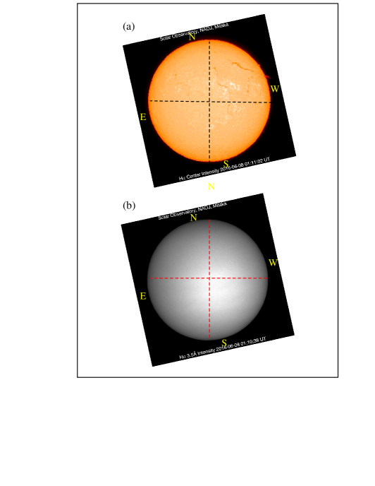
Figure 1.: In the upper and lower panels are shown (a) the H$\alpha+0.0$ Å(line-center) image and (b) the H$\alpha+3.5$ Å(nearly equivalent to continuum) image of the Sun on 2016 June 8, observed by the Solar Flare Telescope at the Solar Observatory, National Astronomical Observatory of Japan. The solar meridian and equator (depicted in dashed lines) are aligned with the vertical and horizontal directions, respectively, in order to maintain consistency with Figure 2.

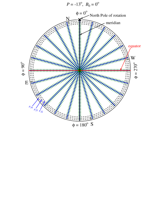
Figure 2.: Graphical description of the observed 840 (= 35$\times$24) points on the solar disk, at which the spectral data were taken. Their locations are specified by 35 radial distances from $r=0$ (disk center) to $r=0.97$ (near to the limb) with a step of $\Delta r=1/35(\simeq 30^{\prime\prime})$ in units of the solar disk radius, and 24 position angles ($\phi$) with an increment of 15^∘. The short segments (in line with alignment of the slit being perpendicular to the radial direction) show the integrated range ($50^{\prime\prime}$) in the spatial direction for each of the spectra.

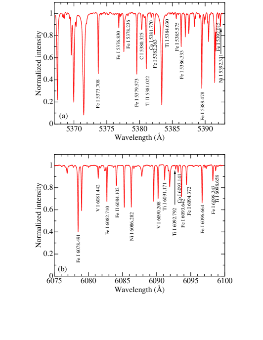
Figure 3.: Examples of our spectra at the disk center ($r=0$, $\phi=0^{\circ}$) in (a) the 5367–5393Å region, and (b) the 6075–6100Å region. The 28 spectral lines we selected are indicated in the figure.

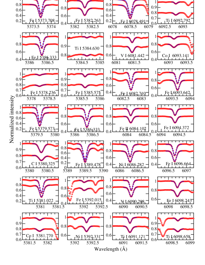
Figure 4.: Comparison of the observed spectrum (open circles) and the fitted theoretical spectrum (solid line) for each of the 28 lines. In each panel, two spectra at the disk-center ($r_{0},\phi_{0}$) and the near-limb ($r_{33},\phi_{0}$) are depicted, where the latter is shifted downward with an offset of 0.2.

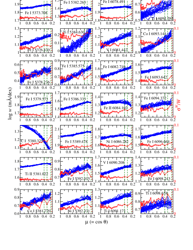
Figure 5.: Solid lines (scale on the left-hand axis): center-to-limb run of $w_{ij}$ [local equivalent width at ($r_{i}$, $\phi_{j}$)] with $\mu_{i}$ ($i=0,1,\cdots,34$) for each of the 24 position angles ($\phi_{j}$, $j=0,1,\cdots,23$) where $\mu_{i}\equiv\cos\theta_{i}\equiv\sqrt{1-(i/35)^{2}}$. Open-circle-connected lines (scale on the right-hand axis of the rightmost panels): center-to-limb run of $\sigma_{i}^{W}/W_{i}$ with $\mu_{i}$, where $W_{i}$ and $\sigma_{i}^{W}$ are the mean $w_{ij}$ averaged over $\phi_{j}$ and its standard deviation, respectively. The positions of $r_{32}$, $r_{33}$, and $r_{34}$ (near-limb regions of our concern) are indicated by the vertical dashed lines.

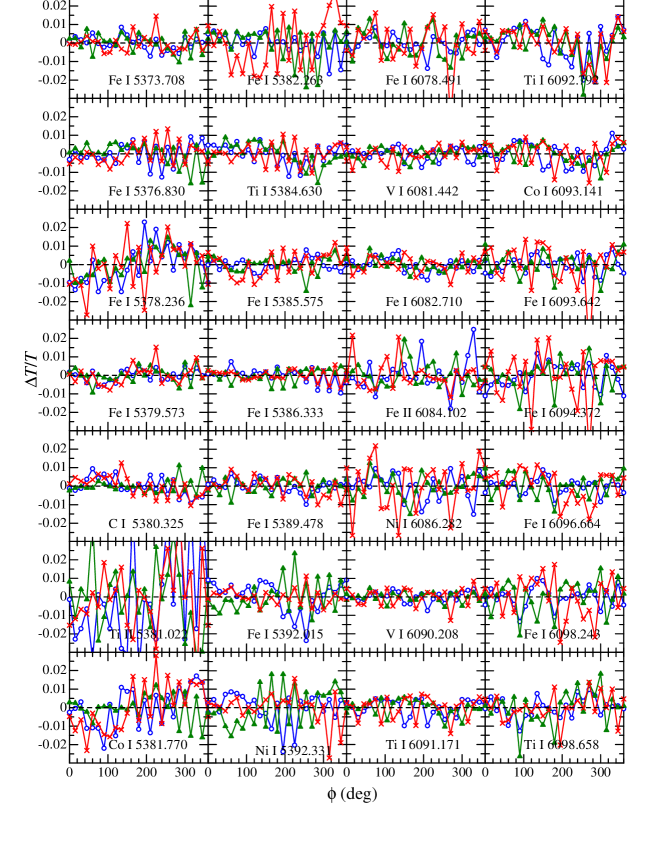
Figure 6.: Run of the temperature fluctuation ($\Delta T/T$) with the position angle $\phi_{j}$ ($j=0,\cdots,23$) near to the limb at $r_{32}$ (open circles), $r_{33}$ (filled triangles), and $r_{34}$ (crosses), which was formally derived from the equivalent-width fluctuation $(\Delta w/w)_{ij}$ by using the $T$-sensitivity parameter ($K_{i}$).

Figure 7.: Values of (a) $\sigma^{W}/W$, (b) $K$, and (c) $(\sigma^{W}/W)/|K|$ for each line plotted against $W$ (all these values correspond to $r_{33}$ near to the limb).

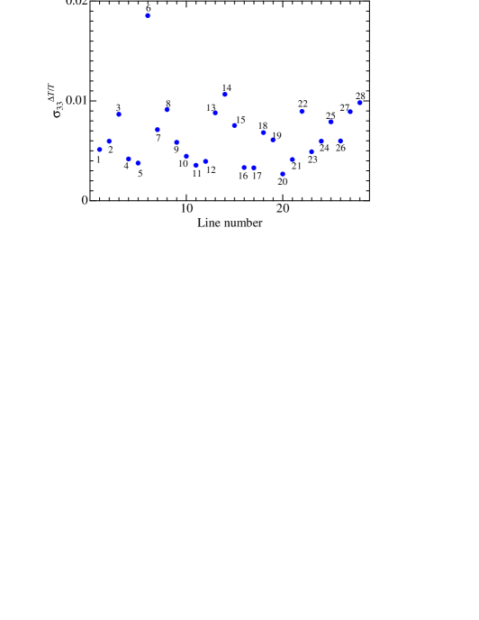
Figure 8.: Standard deviation of $\Delta T/T$ for each line (calculated over the circumference near to the limb at $r_{33}$) plotted against the line number.

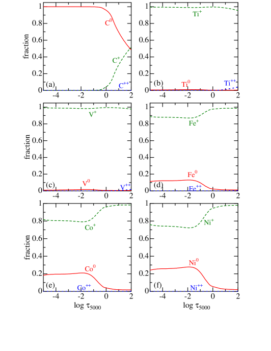
Figure 9.: Number population fractions at the neutral (X⁰; solid line), once-ionized (X⁺; dashed line), and twice-ionized (X⁺⁺; dotted line) stages plotted against the standard continuum optical depth at 5000 Å, which were computed from Kurucz’s (1993) solar model atmosphere. The panels show: (a) C, (b) Ti, (c) V, (d) Fe, (e) Co, and (f) Ni.

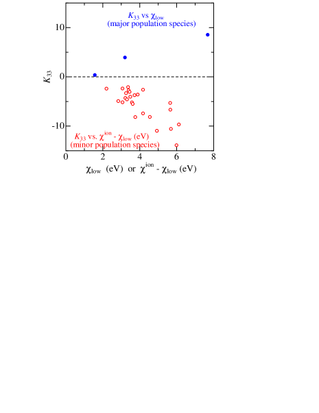
Figure 10.: The $K$ values (temperature sensitivity of the line strength) computed at $r_{33}$ for each line plotted against the critical potential energy. Filled circles: case for the major population species (C i, Ti ii, and Fe ii) with positive $K$, where the abscissa is $\chi_{\rm low}$. Open circles: case for the minor population species (Ti i, V i, Fe i, Co i, and Ni i) with negative $K$, where the abscissa is $\chi^{\rm ion}-\chi_{\rm low}$.

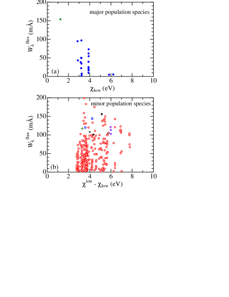
Figure 11.: The solar flux equivalent widths of the 311 lines used by Takeda (1995b) plotted against the critical potential energy. (a) Case of major population species where the abscissa is $\chi_{\rm low}$. Filled triangle: Ti ii, filled circles: Fe ii. (b) Case of minor population species, where the abscissa is $\chi^{\rm ion}-\chi_{\rm low}$. Open triangle: Mg i, open squares: Ca i, open downward triangles: Ti i, open diamond: Cr i, open stars: Mn i, open circles: Fe i, and the cross: Ni i.

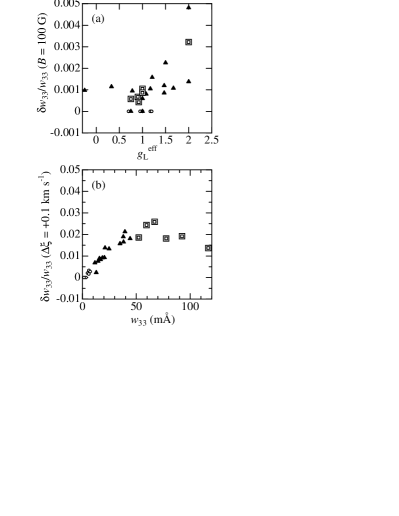
Figure 12.: (a) Computed relative variations of equivalent widths near to the limb ($\delta w_{33}/w_{33}$; at $i=33$, $j=0$) caused by the Zeeman splitting in the presence of a magnetic field of 100 G, plotted against $g_{\rm L}^{\rm eff}$ (effective Landé factor). (b) Computed relative variations of $\delta w_{33}/w_{33}$ caused by by increasing the microturbulence by 0.1 km s^-1 (from 1.0 km s^-1 to 1.1 km s^-1), plotted against $w_{33}$. Different symbols (and sizes) are used according to the strengths of $w_{33}$. Small open circles: $w_{33}<$ 10 mÅ, filled triangles: 10 mÅ$\leq w_{33}<$ 50 mÅ, and large double squares: 50 mÅ$\leq w_{33}$.

References

- [] Brun, A.S., Toomre, J.: 2002, ApJ 570, 865. DOI:10.1086/339228
- [] Cabrera Solana, D., Bellot Rubio, L.R., del Toro Iniesta, J.C.: 2005, A&A 439, 687. DOI:10.1051/0004-6361:20052720
- [] Caccin, B., Donati-Falchi, A., Falciani, R.: 1973, Sol. Phys. 33, 49. DOI:10.1007/BF00152376
- [] Caccin, B., Falciani, R., Donati-Falchi, A.: 1976, Sol. Phys. 46, 29. DOI:10.1007/BF00157553
- [] Caccin, B., Falciani, R., Donati Falchi, A.: 1978, Sol. Phys. 57, 13. DOI:10.1007/BF00152039
- [] Caccin, B., Falciani, R., Moschi, G., Rigutti, M.: 1970, Sol. Phys. 13, 33. DOI:10.1007/BF00963940
- [] Cayrel, R.:1988, in The Impact of Very High S/N Spectroscopy on Stellar Physics, Proc. IAU Symp. 132, eds. G. Cayrel de Strobel and M. Spite (Kluwer, Dordrecht), p.345.
- [] Criscuoli, S., Ermolli, I., Uitenbroek, H., Giorgi, F.: 2013, ApJ 763, 144. DOI:10.1088/0004-637X/763/2/144
- [] Elste, G.: 1986, Sol. Phys. 107, 47. DOI:10.1007/BF00155340
- [] Fabbian, D., Khomenko, E., Moreno-Insertis, F., Nordlund, Å: 2010, ApJ 724, 1536. DOI:10.1088/0004-637X/724/2/1536
- [] Fabbian, D., Moreno-Insertis, F., Khomenko, E., Nordlund, Å: 2012, A&A 548, A35. DOI:10.1051/0004-6361/201219335
- [] Falciani, R., Rigutti, M., Roberti, G.: 1974, Sol. Phys. 35, 277. DOI:10.1007/BF00151948
- [] Gray, D.F.: 2005, The Observation and Analysis of Stellar Photospheres, 3rd ed. (Cambridge University Press, Cambridge).
- [] Gray, D.F., Livingston, W.C.: 1997a, ApJ 474, 798. DOI:10.1086/303479
- [] Gray, D.F., Livingston, W.C.: 1997b, ApJ 474, 802. DOI:10.1086/303489
- [] Holweger, H., Gehlsen, M., Ruland, F.: 1978, A&A 70, 537.
- [] Hotta, H., Rempel, M., Yokoyama, T.: 2015, ApJ 798, 51. DOI:10.1088/0004-637X/798/1/51
- [] Jevremović, D., Vince, I., Erkapić, S., Popović, L.: 1993, Publ. Obs. Astron. Belgrade 44, 33.
- [] Kiselman, D., Pereira, T.M.D., Gustafsson, B., Asplund, M., Meléndez, J., Langhans, K.: 2011, A&A 535, A14. DOI:10.1051/0004-6361/201117553
- [] Kovtyukh, V.V., Gorlova, N.I.: 2000, A&A 358, 587.
- [] Kuhn, J.R., Bush, R.I., Scheick, X., Scherrer, P.: 1998, Nature 392, 155. DOI:10.1038/32361
- [] Kurucz, R.L.: 1993, Kurucz CR-ROM No. 13, Harvard-Smithsonian Center for Astrophysics, Cambridge, MA.
- [] Miesch, M.S., Brun, A.S., Toomre, J.: 2006, ApJ 641, 618. DOI:10.1086/499621
- [] Moore, C.S., Uitenbroek, H., Rempel, M., Criscuoli, S., Rast, M.P.: 2015, ApJ 799, 150. DOI:10.1088/0004-637X/799/2/150
- [] Muller, R., Hanslmeier, A., Utz, D.: 2017, A&A 598, A6. DOI:10.1051/0004-6361/201527736
- [] Nakai, Y., Hattori, A.: 1985, Memoirs of the Faculty of Science, Kyoto University, Series A of Physics, Astrophysics, Geophysics and Chemistry 36, 385.
- [] Nordlund, Å., Stein, R.F., Asplund, M.: 2009, Living Rev. Solar Phys. 6, 2. DOI:10.12942/lrsp-2009-2
- [] Noyes, R.W., Ayres, T.R., Hall, D.N.B: 1973, Sol. Phys. 28, 343. DOI:10.1007/BF00152303
- [] Pereira, T.M.D., Asplund, M., Kiselman, D.: 2009, A&A 508, 1403. DOI:10.1051/0004-6361/200912840
- [] Petrie, G.J.D.: 2015, Living Rev. Solar Phys. 12, 5. DOI:10.1007/lrsp-2015-5
- [] Rast, M.P., Ortiz, A., Meisner, R.W.: 2008, ApJ 673, 1209. DOI:10.1086/524655
- [] Rodríguez Hidalgo, I., Collados, M., Vázquez, M.: 1992, A&A 264, 661.
- [] Rodríguez Hidalgo, I., Collados, M., Vázquez, M.: 1994, A&A 283, 263.
- [] Rutten, R.J.: 1973, Sol. Phys. 28, 347. DOI:10.1007/BF00152304
- [] Ryabchikova, T., Piskunov, N., Kurucz, R.L., Stempels, H.C., Heiter, U., Pakhomov, Yu, Barklem, P.S.: 2015, Phys. Scr. 90, 054005. DOI:10.1088/0031-8949/90/5/054005
- [] Sánchez Almeida, J., Martínez González, M.: 2011, in Solar Polarization 6, ASP Conf. Ser., eds. J.R. Kuhn, D.M. Harrington, H. Lin, S.V. Berdyugina, J. Trujillo-Bueno, S.L. Keil, and T. Rimmele 437, 451 (Astron. Soc. Pacific: San Francisco).
- [] Scherrer, P.H., Bogart, R.S., Bush, R.I., Hoeksema, J.T., Kosovichev, A.G., Schou, J., Rosenberg, W., Springer, L., Tarbell, T.D., Title, A., Wolfson, C.J., Zayer, I., MDI Engineering Team: 1995, Sol. Phys. 162, 129. DOI: 10.1007/BF00733429
- [] Sheminova, V.A.: 1993, Kin. Fiz. Neb. Tel. 9, 27.
- [] Sheminova, V.A.: 1998, A&A 329, 721.
- [] Stenflo, J.O., Lindegren, I.: 1977, A&A 59, 367.
- [] Takeda, Y.: 1993, PASJ 45, 453.
- [] Takeda, Y.: 1994, PASJ 46, 53.
- [] Takeda, Y.: 1995a, PASJ 47, 287.
- [] Takeda, Y.: 1995b, PASJ 47, 337.
- [] Takeda, Y., Ohkubo, M., Sadakane, K.: 2002, PASJ 54, 451. DOI:10.1093/pasj/54.3.451
- [] Takeda, Y., UeNo, S.: 2014, PASJ 66, 32. DOI:10.1093/pasj/psu001
- [] Takeda, Y., UeNo, S.: 2017, PASJ 69, 46. DOI:10.1093/pasj/psx022
- [] Trujillo Bueno, J., Shchukina, N., Asensio Ramos, A.: 2004, Nature 430, 326. DOI:10.1038/nature02669
- [] Tsuneta, S., Ichimoto, K., Katsukawa, Y., Nagata, S., Otsubo, M., Shimizu, T., Suematsu, Y., Nakagiri, M., Noguchi, M., Tarbell, T., Title, A., Shine, R., Rosenberg, W., Hoffmann, C., Jurcevich, B., Kushner, G., Levay, M., Lites, B., Elmore, D., Matsushita, T., Kawaguchi, N., Saito, H., Mikami, I., Hill, L.D., Owens, J.K.: 2008, Sol. Phys. 249, 167. DOI: 10.1007/s11207-008-9174-z
- [] Ulrich, R.K., Boyden, J.E.: 2005, ApJ 620, L123. DOI:10.1086/428724