Complete analysis of ensemble inequivalence in the Blume-Emery-Griffiths model

Abstract

We study inequivalence of canonical and microcanonical ensembles in the mean-field Blume-Emery-Griffiths model. This generalizes previous results obtained for the Blume-Capel model. The phase diagram strongly depends on the value of the biquadratic exchange interaction $K$, the additional feature present in the Blume-Emery-Griffiths model. At small values of $K$, as for the Blume-Capel model, lines of first and second order phase transitions between a ferromagnetic and a paramagnetic phase are present, separated by a tricritical point whose location is different in the two ensembles. At higher values of $K$ the phase diagram changes substantially, with the appearance of a triple point in the canonical ensemble which does not find any correspondence in the microcanonical ensemble. Moreover, one of the first order lines that starts from the triple point ends in a critical point, whose position in the phase diagram is different in the two ensembles. This line separates two paramagnetic phases characterized by a different value of the quadrupole moment. These features were not previously studied for other models and substantially enrich the landscape of ensemble inequivalence, identifying new aspects that had been discussed in a classification of phase transitions based on singularity theory. Finally, we discuss ergodicity breaking, which is highlighted by the presence of gaps in the accessible values of magnetization at low energies: it also displays new interesting patterns that are not present in the Blume-Capel model.

I Introduction

In the last couple of decades it has become progressively clear that systems with long-range interactions show peculiar properties Campa14 . For such systems, the interaction between constituents decays, at large distance $r$, as $r^{-\alpha}$, with $\alpha$ smaller than space dimension $d$.

The most prominent property of these systems at thermodynamic equilibrium is ensemble inequivalence Barre01 : phase diagrams can be different in the canonical and microcanonical ensembles, This property directly stems from the non additivity of the energy. There are cases, however, in presence of only second order transitions in both ensembles, where inequivalence does not occur Barre01 ; touch04 .

Self-gravitating systems Binney can be considered as the paradigmatic example of long-range interactions. One of the most important consequences of ensemble inequivalence, i.e. negative specific heat in the microcanonical ensemble, has been found in self-gravitating systems already about half a century ago Antonov62 ; Lydnen-Bell68 ; Thirring70 . When an isolated system has a negative specific heat, an increase in its temperature is associated to a decrease of its energy. In a self-gravitating system this occur when, e.g, a contraction of a globular cluster is accompanied by an increase of the average kinetic energy of its members. However, it is now evident that there are other numerous examples of long-range systems in nature: Coulomb systems like plasmas nicholson , trapped cold atoms Morigi , two-dimensional geophysical and hydrodynamic flows bouchet , dipolar media Bramwell , nuclear matter chomaz ; foot6 .

The investigation of the properties of long-range interacting systems has often been pursued with the use of simplified models, more amenable to a complete study, that can present the most important features of more realistic systems. Spin systems with mean-field interactions (i.e., with each spin interacting with equal strength with all the others) constitute a good example. Indeed, ensemble inequivalence was first discussed for the spin-1 mean-field Blume-Capel (BC) model Blume66 in Ref. Barre01 . It has been shown that the two-dimensional phase diagram $(\Delta,T)$, where $T$ is temperature and $\Delta$ the single-spin energy parameter, exhibits a tricritical point where a line of second order transitions meets a line of first order transitions. However, both the location of the tricritical point and the one of first order transitions are different in the canonical and microcanonical ensembles. Regions of negative specific heat are present in the microcanonical ensemble in correspondence to a first order transition in the canonical ensemble. It can be seen that these features are quite common in mean-field systems Campa09 .

A physically relevant generalization of the Blume-Capel model is the Blume-Emery-Griffiths (BEG) model Blume71 . This latter was introduced as a simplified model to study phase separation and superfluid transitions in $He^{3}-He^{4}$ mixtures. It consists of a system of spin-1 variables $S_{i}$ on a three-dimensional lattice with nearest neighbour interactions. The value $S_{i}=0$ corresponds to the presence on site $i$ of a $He^{3}$ atom, while the values $S_{i}=1$ and $S_{i}=-1$ are associated with the presence of a $He^{4}$ atom (the additional degree of freedom is justified by physical observations Blume71 ). The analytical study was performed in the mean-field approximation in the canonical ensemble. The same results can be obtained considering mean-field interactions, i.e. putting the model on a fully connected infinite-range lattice.

The solution in the microcanonical ensemble of the mean-field BEG model has never been performed and the corresponding ensemble inequivalence never discussed in the literature. Moreover, in spite of the numerous studies on ensemble inequivalence, the investigation has been mostly restricted to phase diagrams with tricritical points. However, it is well known that more complex phase diagrams showing inequivalence can exist bouchet05 .

Recently, the solution of the Thirring model Thirring70 has been presented in full detail campa2016 and it has been shown that the phase diagram presents lines of first order transitions terminating at critical points. However, the location of the critical point is not the same in the canonical and microcanonical phase diagrams.

The motivation of this work is to extend the study of ensemble inequivalence to more complex situations like the BEG model. The presence of a further parameter with respect to the BC model, i.e. the coefficient of the biquadratic interaction, determines the occurrence of a much more complex phase diagram made of critical, tricritical and triple points, lines of second and first order transitions. In the canonical ensemble these features have been already studied in Refs. Blume71 ; Hoston . By studying the system also in the microcanonical ensemble, our purpose here is to show that ensemble inequivalence manifests itself in various different interesting ways.

The paper is organized as follows: in Sec. II we describe in detail the solution of the BEG model in the canonical ensemble by means of the Gaussian identity. In Sec. III the solution of the model in the microcanonical ensemble is presented. In Sec. IV the most interesting features of the model are discussed and the analysis of ensemble inequivalence for the canonical and microcanonical ensembles is completed. In Sec. V we study ergodicity breaking, another important feature often present in long-range systems. Finally, some conclusions are briefly mentioned in Sec. VI.

II The model and its solution in the canonical ensemble

Let us consider the infinite range Blume-Emery-Griffiths Blume71 model in the absence of external magnetic field. The Hamiltonian of the model is

$$H=\Delta\sum_{i=1}^{N}S_{i}^{2}-\frac{J}{2N}\left(\sum_{i=1}^{N}S_{i}\right)^{2}-\frac{K}{2N}\left(\sum_{i=1}^{N}S_{i}^{2}\right)^{2},$$ (1)

where $\Delta$ is the single-spin energy parameter (single-ion anisotropy) controlling the energy difference between the ferromagnetic ($S_{i}=\pm 1$) and the paramagnetic ($S_{i}=0$) states, while $J$ and $K$ are the bilinear and the biquadratic exchange interaction parameters, respectively. The partition function reads

$$Z(\beta,N)=\sum_{\{S_{i}\}}e^{-\beta\Delta\sum_{i=1}^{N}S_{i}^{2}+\frac{\beta J}{2N}\left(\sum_{i=1}^{N}S_{i}\right)^{2}+\frac{\beta K}{2N}\left(\sum_{i=1}^{N}S_{i}^{2}\right)^{2}}\,,$$ (2)

where $\beta=(k_{B}T)^{-1}$, $k_{B}$ is Boltzmann’s constant and $T$ is the absolute temperature. In the following we use units in which $k_{B}=1$. Furthermore, without loss of generality, we can take $J=1$ (this formally amounts to the substitutions $\beta\to\beta J$, $\Delta\to\Delta/J$ and $K\to K/J$). Using the Gaussian identity

$$\mathrm{exp}(ba^{2})=\sqrt{\frac{b}{\pi}}\int^{+\infty}_{-\infty}\mbox{d}x\,\mathrm{exp}(-bx^{2}+2abx),$$ (3)

one can then rewrite the partition function of the system as (Hubbard-Stratonovich transformation)

$$Z(\beta,N) =\frac{N\beta\sqrt{K}}{2\pi}\sum_{\{S_{i}\}}e^{-\beta\Delta\sum_{i=1}^{N}S_{i}^{2}}$$

$$\times \!\!\!\!\!\!\int^{+\infty}_{-\infty}\mbox{d}x\,\int^{+\infty}_{-\infty}\mbox{d}y\,e^{-\frac{\beta N}{2}x^{2}-\frac{\beta NK}{2}y^{2}+\beta Nmx+\beta NKqy}\,,$$

where $m=\sum_{i}S_{i}/N$ and $q=\sum_{i}S_{i}^{2}/N$ are the magnetization and the quadrupole moment per particle, respectively. Performing the sum over ${\{S_{i}\}}$ we get

$$Z(\beta,N)=\frac{N\beta\sqrt{K}}{2\pi}\int\int^{+\infty}_{-\infty}\mbox{d}x\mbox{d}y\,e^{-N\beta\tilde{f}(\beta,x,y)}\,,$$ (5)

where

$$\beta\tilde{f}(\beta,x,y) = \frac{\beta}{2}\left(x^{2}+Ky^{2}\right)$$ (6)

$$- \ln\left[1+2e^{-\beta\Delta+\beta Ky}\cosh\beta x\right]\,.$$

The integral in Eq. 5 can be performed using Laplace (saddle point) method, which in the limit $N\rightarrow\infty$ gives the expression of the free energy per particle

$$f(\beta)=\min_{x,y}\tilde{f}(\beta,x,y).$$ (7)

The partial derivatives of $\tilde{f}$ with respect to $x$ and $y$ vanish in the saddle point, giving:

$$x=\frac{2\sinh\beta x}{\exp\left(\beta\Delta-\beta Ky\right)+2\cosh\beta x},$$ (8)

$$y=\frac{2\cosh\beta x}{\exp\left(\beta\Delta-\beta Ky\right)+2\cosh\beta x}.$$ (9)

Furthermore the Hessian matrix of $\tilde{f}$ must be positive definite at the values of $x$ and $y$ that solve these equations. If there is more than one solution, the relevant one for the equilibrium state is that realizing the absolute minimum of $\tilde{f}$. One can easily see that these values of $x$ and $y$ correspond to the equilibrium magnetization $m$ and quadrupole moment $q$, respectively. Using Eqs. (8) and (9), it can be shown that, when $x\neq 0$, the magnetization and the quadrupole moment at equilibrium are related by

$$y=x\coth\beta x.$$ (10)

This relation will turn out to be useful in the following.

We begin the study of the thermodynamic phase diagram of the system by considering two particular cases, i.e. $\Delta=0$ and $T=0$.

Let us first consider the case $\Delta=0$. It is not difficult to see that in this case the system exhibits a second order phase transition, by increasing $T$, from a ferromagnetic ($m\neq 0$) to a paramagnetic ($m=0$) phase. In fact, for $\Delta=0$ the right hand side of Eq. (8) has, as a function of $x$, a positive definite first derivative and a negative definite second derivative for $x>0$. This implies that there is a second order phase transition at the value of $\beta$ where the $x$ derivative of this function at $x=0$ is equal to $1$. In evaluating this derivative we have to take the value of $y$ equal to the limit of Eq. (10) for $x\to 0$, i.e., $y=1/\beta$. Then, the critical $\beta$ value is obtained as $\beta_{c}(\Delta=0)=1+e^{-K}/2$, i.e., $T_{c}(\Delta=0)=(1+e^{-K}/2)^{-1}$. This is, consistently, the value of $\beta$ for which Eq. (9) has the solution $y=1/\beta$ for $x=0$.

On the other hand, for $T=0$ the system exhibits a first order phase transition. In fact, for $T=0$ the equilibrium state is the one of minimum energy. It is easy to see that the minimum energy state is the fully magnetized state with $m=1$ or $m=-1$ (i.e., $S_{i}=1$ $\forall i$ or $S_{i}=-1$ $\forall i$) and $q=1$ when $\Delta<(K+1)/2\equiv\Delta_{c}$, while it is the paramagnetic state with $m=q=0$ (i.e., $S_{i}=0$ $\forall i$) when $\Delta>(K+1)/2$. Thus, in the $(\Delta,T)$ phase diagram we have, for any given $K$, a second order transition at the point $(0,T_{c})$ and a first order transition at the point $(\Delta_{c},0)$. We should then expect to find, in the phase diagram, both a line of second order transitions and a line of first order transitions as a continuation of these two extreme cases. We now show that this is the case.

The critical line of second order transitions from a ferromagnetic ($m\neq 0$) state to a paramagnetic ($m=0$) state can be obtained following Landau theory of phase transitions. If $\tilde{f}$ would depend, as far as order parameters are concerned, only on $x$, we know that the critical points would be given by $\partial\tilde{f}/\partial x=\partial^{2}\tilde{f}/\partial x^{2}=\partial^{3}\tilde{f}/\partial x^{3}=0$, with $\partial^{4}\tilde{f}/\partial x^{4}>0$. Since in our case $\tilde{f}$ depends on $x$ and $y$, the critical points, besides satisfying Eqs. (8) and (9), should make the determinant of the Hessian matrix vanish, i.e. $(\partial^{2}\tilde{f}/\partial x^{2})(\partial^{2}\tilde{f}/\partial y^{2})-(\partial^{2}\tilde{f}/\partial x\partial y)^{2}=0$. Besides that, we require the vanishing of the third order variation and the positiveness of the fourth order variation of $\tilde{f}$ along a particular path on the $(x,y)$ plane passing through the given equilibrium point. Details of this procedure are given in Appendix A; here we just give the result. The third order variation, for the solutions of Eqs. (8) and (9) with $x=0$, identically vanishes since $\tilde{f}$ is an even function of $x$. We are left with the vanishing of the Hessian and the positiveness of the fourth order variation; these conditions are expressed by

$$A_{c}=\exp(\beta\Delta-K)+2-2\beta = 0$$ (11)

$$B_{c}=-\beta\left(1+2K\right)+\left(3+2K\right) > 0$$ (12)

From Eq. (11) we get the equation of the critical line in the $(\Delta,T)$ phase diagram as

$$\beta=\frac{1}{2}e^{\beta\Delta-K}+1\,.$$ (13)

For the particular case $\Delta=0$ we obtain the value $\beta_{c}=1/T_{c}$ given above. Eq. (12) gives

$$\beta<\frac{3+2K}{1+2K}\,.$$ (14)

The equality in the last equation gives the value of $\beta$ at the canonical tricritical point (CTP), i.e., the point where the line of second order transitions ends and the line of first order transitions begins. It is characterized by the vanishing of both the second order and the fourth order variations of $\tilde{f}$. In terms of the temperature $T$

$$T_{CTP}=\frac{1+2K}{3+2K}\,,$$ (15)

and the value of $\Delta$ at the tricritical point is then obtained by Eq. (13) as

$$\Delta_{CTP}=T_{CTP}\ln\frac{4e^{K}}{1+2K}\,.$$ (16)

After the tricritical point the first order transition line has to be computed numerically: the function $\tilde{f}(\beta,x,y)$ has local minima, in the $(x,y)$ plane, both at $x=0$ and at $x\neq 0$, the former corresponding to a paramagnetic phase and the latter to a ferromagnetic phase. The equilibrium state is the one corresponding to the global minimum (with the magnetization $m$ equal to the $x$ of the global minimum). The points of the $(\Delta,T)$ phase diagram where the two local minima are equal give the first order transition line. In Fig. 1 we show the phase diagram for two cases, $K=0$ and $K=1$.

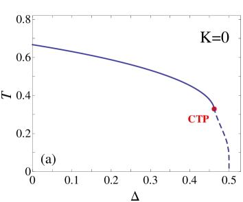
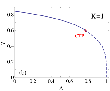
Figure 1: $(\Delta,T)$ phase diagram of the BEG model in the canonical ensemble for two different values of the biquadratic interaction parameter $K$. Solid and dashed lines are second and first order phase transition lines, respectively, while the red dot denotes the canonical tricritical point (CTP). (a) $K=0$, i.e. the BC model, $\Delta_{CTP}\backsimeq 0.4621$, $T_{CTP}=1/3$; (b) $K=1$, $\Delta_{CTP}\backsimeq 0.7726$, $T_{CTP}=0.6$.

We will see that for larger values of $K$ the phase diagram is more complex. The new main feature is the appearance of a triple point from which three lines of first order transitions depart. One of them, which separates two paramagnetic phases, ends in a critical point. For even larger values of $K$ the tricritical point disappears, since the critical line branches in two lines of first order transitions before reaching the tricritical point. Details will be given in Sec. IV, while treating ensemble inequivalence. We now turn to the study of the microcanonical phase diagram.

III Solution in the microcanonical ensemble

Now, let us consider the BEG model in microcanonical ensemble. Suppose that, in the macroscopic system with $N$ particles, $N_{+}$, $N_{-}$ and $N_{0}$ are the number of particles with up, down and zero spins, respectively, with $N=N_{+}+N_{-}+N_{0}$. The energy $E$ of the system can be expressed as a function of these occupation numbers as

$$E=\Delta Q-\frac{1}{2N}M^{2}-\frac{K}{2N}Q^{2},$$ (17)

where $M=\sum_{i=1}^{N}S_{i}=N_{+}-N_{-}$ and $Q=\sum_{i=1}^{N}S_{i}^{2}=N_{+}+N_{-}$ are the magnetic and quadrupole moments. The number $W$ of microscopic configurations with macroscopic occupation numbers $N_{+}$, $N_{-}$ and $N_{0}$ is

$$W=\frac{N!}{N_{+}!N_{-}!N_{0}!}.$$ (18)

The associated entropy $S=\ln W$ can be computed in the thermodynamic limit $N\rightarrow\infty$ using Stirling’s approximation. We obtain

$$S = -N\left[(1-q)\ln(1-q)+\frac{1}{2}(q+m)\ln(q+m)\right.$$ (19)

$$+ \left.\frac{1}{2}(q-m)\ln(q-m)-q\ln 2\right]\,,$$

where $m=M/N$ and $q=Q/N$ are the single-site magnetization and quadrupole moment. This is not yet the equilibrium entropy, which is given by optimizing the macroscopic occupation numbers at fixed energy $E$ foot7 . To this purpose, let us introduce the single-site energy $\epsilon=E/N$ and rewrite Eq. (17) as

$$q^{2}-2\frac{\Delta}{K}q+\frac{2\epsilon}{K}+\frac{m^{2}}{K}=0\,.$$ (20)

Eq. (20) is a quadratic equation with respect to $q$ with solutions

$$q_{\pm}=\frac{\Delta}{K}\pm\sqrt{\left(\frac{\Delta}{K}\right)^{2}-\frac{2\epsilon}{K}-\frac{m^{2}}{K}}\,.$$ (21)

Obviously the range of variation of the energy $\epsilon$ must be such that the expression under square root in the last equation is never negative (the bounds of $\epsilon$ will be discussed in detail in Sec. V, dedicated to ergodicity breaking). Moreover, at least one between the quantities $q_{+}$ and $q_{-}$ must lie in the interval $[0,1]$; when one of the two is not between $0$ and $1$ only the other can be accepted as solution of Eq. (20). Note that in the limit $K\rightarrow 0$ only the solution $q=q_{-}$ survives, coinciding with the expression of the quadrupole moment of the BC model Barre01 . However, for a generic value of $K$ we need to consider both solutions. Substituting these solutions into Eq. (19) we obtain two expressions for the single-site entropy $S/N$ as a function of the magnetization $m$ and the energy $\epsilon$: $\tilde{s}_{\pm}(\epsilon,m)$. The equilibrium entropy is given by $s(\epsilon)=\max\{s_{+}(\epsilon),s_{-}(\epsilon)\}$, where $s_{\pm}(\epsilon)=\max_{m}\tilde{s}_{\pm}(\epsilon,m)$. The value of $m$ solving this extremum problem is the equilibrium spontaneous magnetization. Thus, the maximum of $\tilde{s}_{\pm}(\epsilon,m)$ is given by

$$\frac{\partial\tilde{s}_{\pm}(\epsilon,m)}{\partial m}=\ln\left[\frac{2(1-q_{\pm})}{\sqrt{q_{\pm}^{2}-m^{2}}}\right]\frac{\partial q_{\pm}}{\partial m}+\frac{1}{2}\ln\left[\frac{q_{\pm}-m}{q_{\pm}+m}\right]=0\,,$$ (22)

where the derivative of $q_{\pm}$ with respect to $m$ is computed from Eq. (21), and with the further condition that $\frac{\partial^{2}\tilde{s}_{\pm}(\epsilon,m)}{\partial m^{2}}<0$. As for the canonical case, if there is more than one solution, the relevant one for the equilibrium state realizes the absolute maximum.

In Fig. 2 we plot, as an example, $\tilde{s}_{-}(\epsilon,m)$ as a function of $m$ for given values of $\epsilon$, for $K=1$ and for two different values of $\Delta$. In these cases the function $\tilde{s}_{-}(\epsilon,m)$ is the one giving the absolute maximum. The figure shows the behavior of the function at increasing energy when there is a second order transition ($\Delta=0.8$) or a first order transition ($\Delta=0.93$).

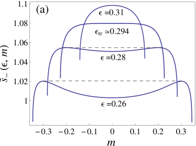
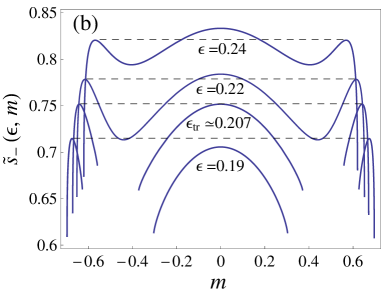
Figure 2: Entropy $\tilde{s}_{-}(\epsilon,m)$ vs. magnetization $m$ for $K=1$ and for two values of the single-spin energy parameter $\Delta$, plotted for several different values of the energy. (a) $\Delta=0.8$: second order phase transition. (b) $\Delta=0.93$: first order phase transition; at the transition energy the maxima at $m=0$ and at $m\neq 0$ are at the same height.

Similarly to the canonical case, the critical line for the transition between ferromagnetic and paramagnetic states is found exploiting the Landau theory of phase transitions. This is done by expanding $\tilde{s}_{\pm}(\epsilon,m)$ in powers of $m$. Contrary to the canonical case, where we had to minimize a function, $\tilde{f}(\beta,x,y)$, with respect to two variables, now we have to maximize only with respect to the variable $m$, since $q$ is a function of $\epsilon$ and $m$. Correspondingly, the expansion for the Landau theory concerns only the variable $m$. Because of the invariance under change of sign, $m\to-m$, we obtain an expression of the form

$$\tilde{s}_{\pm}(\epsilon,m)=s_{0}+A_{m}m^{2}+B_{m}m^{4}+O(m^{6}),$$ (23)

where the zero magnetization entropy $s_{0}$ is

$$s_{0}=-(1-z_{\pm})\ln(1-z_{\pm})-z_{\pm}\ln z_{\pm}+z_{\pm}\ln 2\,,$$ (24)

with $z_{\pm}=\Delta/K\pm\sqrt{(\Delta/K)^{2}-2\epsilon/K}$, and the coefficients are given by

$$A_{m} = \mp a\ln\frac{2(1-z_{\pm})}{z_{\pm}}-\frac{1}{2z_{\pm}},$$ (25)

$$B_{m} = \mp b\ln\frac{2(1-z_{\pm})}{z_{\pm}}-\frac{a^{2}}{2z_{\pm}(1-z_{\pm})}$$ (26)

$$\mp\frac{a}{2z_{\pm}^{2}}-\frac{1}{12z_{\pm}^{3}},$$

with $a=\left(4\Delta^{2}-8K\epsilon\right)^{-\frac{1}{2}}$ and $b=Ka^{3}$. We observe that $z_{\pm}$ is equal to $q_{\pm}$ for $m=0$. The critical line is defined by $A_{m}=0$ with $B_{m}<0$. To obtain the critical line in the $(\Delta,T)$ plane we use the expression

$$\frac{1}{T}=\frac{\partial s}{\partial\epsilon}\,.$$ (27)

On the critical line $m=0$, therefore

$$\frac{1}{T}=\frac{\partial s_{0}}{\partial\epsilon}=\mp 2a\ln\frac{2(1-z_{\pm})}{z_{\pm}}\,.$$ (28)

For positive temperatures $T$ foot1 , this equation gives some constraints on the admissible values of $z_{-}$ and $z_{+}$ on the critical line (or, in this respect, for the values of $q_{-}$ and $q_{+}$ in all cases where the equilibrium magnetization $m$ is equal to zero). In particular, the argument of the logarithm must be smaller (larger) than $1$ for $z_{+}$ ($z_{-}$), i.e. $z_{+}>2/3$ ($z_{-}<2/3$). However, the positivity of $T$ is assured by the condition that $A_{m}$ must vanish on the critical line. In fact, the condition $A_{m}=0$ gives, using Eqs. (25) and (28), $z_{\pm}=T$. Substituting $z_{\pm}$ with $T=1/\beta$ in Eq. (28) and in the expression of $a$ we obtain

$$\beta=\frac{1}{2}e^{\beta\Delta-K}+1\,,$$ (29)

i.e., the same expression of the canonical ensemble, that in addition shows that $\beta$ is indeed positive. As explained above, the further condition $B_{c}>0$, valid for the canonical case, is replaced by $B_{m}<0$, so that the critical line ends when $B_{m}=0$, that characterizes the microcanonical tricritical point. It can be proved that $B_{m}<0$ whenever $B_{c}>0$, meaning that the microcanonical critical line extends further with respect to the canonical critical line. These findings are consistent with the general result that for any system the microcanonical critical line includes and extends beyond the canonical critical line Campa09 . This in turn is consistent with the fact that at the points of the phase diagram where there is a canonical second order transition ensembles are equivalent Barre01 ; touch04 . In Appendix B we give some details of the computation of the microcanonical tricritical point, characterized by the values $\Delta_{MTP}$ and $T_{MTP}$, explicitly given in Sec. IV for different values of $K$.

As for the canonical case, after the tricritical point the first order transition line has to be computed numerically. Furthermore, also in this ensemble, by increasing $K$, a line of first order transitions, ending in an isolated critical point, between different paramagnetic states, appears, and the tricritical point disappears, with the critical line branching in two first order transition lines. Details are given in the next Section. However, these relevant points will be different in the two ensembles, showing a marked ensemble inequivalence. Just to anticipate one of the results, contrary to the canonical case, in the microcanonical ensemble the appearance of the critical point and the disappearance of the tricritical point occur at the same value of $K$.

IV Ensemble inequivalence

In this Section we show the complete analysis of ensemble inequivalence. The Section is divided in six Subsections. Depending on the range where the value of $K$ is situated, we have four different situations for the structure of the phase diagrams, and in all cases there is inequivalence. The boundaries of these ranges of $K$ are obtained numerically. The first notable value of $K$ is $K_{1}\backsimeq 2.775$, which is where, in the canonical ensemble, the triple and critical points appear. The value $K_{2}=3$ is where the microcanonical tricritical point disappears. Finally at the value $K_{3}\backsimeq 3.801$ the canonical tricritical point disappears. In the first four Subsections we treat, separately, each one of the cases. The fifth Subsection treats briefly the case of negative temperatures, that can occur in systems with upper bounded energy TGBtemp . A short discussion of the results presented in the first four Subsections, in the framework of the classification of phase transitions as studied in Ref. bouchet05 , is presented in the last Subsection.

IV.1 Low values of $K$: $0\leq K<K_{1}\backsimeq 2.775$

We treat this case by showing the results for $K=1$. The structure of the phase diagram for other values of $K$ in this range is the same. The upper panel of Fig. 3 shows the $(\Delta,T)$ phase diagram in the microcanonical ensemble for $K=1$. The value of $T$ is obtained from Eq. (27). The second order transition changes to first order at the microcanonical tricritical point (MTP). The canonical phase diagram for $K=1$ was shown in the lower panel of Fig. 1. To have a better comparison the two diagrams are now plotted together in the lower panel of Fig. 3, that shows the zoom of the most interesting region. In this plot the second order transitions are denoted by full lines, while the first order transitions are indicated by dashed lines. As anticipated above, the microcanonical critical line extends further with respect to the canonical one. The second order phase transition line is common to both ensembles up the canonical tricritical point (CTP). After this point the canonical ensemble has first order transitions (red dashed line), while for the microcanonical ensemble the second order transition line continues up to the microcanonical tricritical point (MTP). The microcanonical first order transitions are characterized by a temperature jump bouchet05 ; Campa09 , and for this reason the plot has correspondingly two branches.

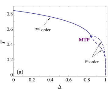
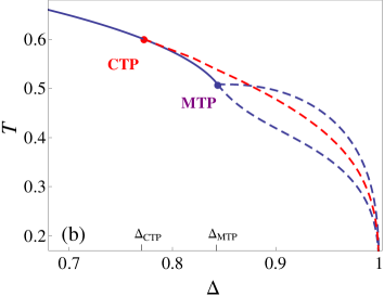
Figure 3: (a) $(\Delta,T)$ phase diagram of the BEG model in the microcanonical ensemble at $K=1$. Solid and dashed lines are the second and first order phase transition lines, respectively. The second order transition line ends at the microcanonical tricritical point (MTP), located at $\Delta_{MTP}\backsimeq 0.8439$, $T_{MTP}\backsimeq 0.5078$. (b) Zoom of the region of the first order transitions, showing also the canonical tricritical point (CTP), located at $\Delta_{CTP}\backsimeq 0.7726$, $T_{CTP}=0.6$, and the canonical first order transition line (red dashed line). The coordinates of the tricritical points in the phase diagram can be calculated from Eqs. (15), (16), (B) and (44). The first order lines reach the $T=0$ line at $\Delta=(K+1)/2=1$.

A further illustration of ensemble inequivalence is given by the caloric curves, i.e., the plots showing temperature $T$ as a function of energy $\epsilon$. In Fig. 4 we show the caloric curves for $K=1$ for several values of $\Delta$, ranging from the value at the canonical tricritical point to the value where the first order transition lines meet the $T=0$ axis (see Fig. 3). Let us remind that in the canonical ensemble $T$ is the control variable and $\epsilon$ is obtained from the thermodynamic expression $\epsilon=\partial\left(\beta f(\beta)\right)/\partial\beta$. In Fig. 4 the microcanonical curves are plotted in blue; in the energy ranges where ensembles are equivalent, these curves represent also the canonical ensemble, while in the inequivalence ranges the canonical curves are given by the red horizontal lines (Maxwell construction), showing the canonical first order transitions.

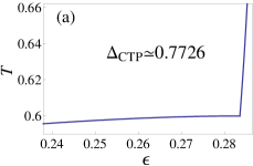
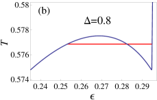
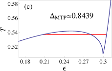
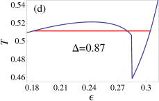
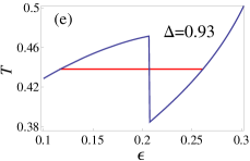
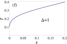
Figure 4: Energy dependence of the temperature (caloric curve) for $K=1$ and different values of the single-spin energy parameter $\Delta$. The blue lines are the microcanonical curves; they coincide with the canonical ones in the energy ranges where ensembles are equivalent. Where instead the ensembles are inequivalent, the canonical curves are given by the horizontal red lines (Maxwell construction). The energies within the range covered by these lines are forbidden in the canonical ensemble.

The second order transition is associated to a discontinuity in the first derivative of the caloric curve. Fig. 4(a) shows the caloric curve at the canonical tricritical point. In this case the low energy branch has a zero slope at the transition point, denoting a diverging specific heat. Increasing $\Delta$, in the range between the canonical and the microcanonical tricritical points, the transition is second order in the microcanonical ensemble and first order in the canonical ensemble, while one can observe the appearance of a negative specific heat $(\partial T/\partial\epsilon<0)$ in the microcanonical ensemble (Fig. 4(b)). At the microcanonical tricritical point (Fig. 4(c)) $\partial T/\partial\epsilon$ diverges in the low energy branch, indicating a vanishing specific heat. For $\Delta>\Delta_{MTP}$ the transition becomes first order also in the microcanonical ensemble, characterized by a temperature jump at the transition energy (Fig. 4(d)). We observe that the temperature jump is negative (by increasing energy), a fact that can be proved on general grounds on the basis of singularity theory for maximization problems bouchet05 ; however, this can also be understood more simply using a heuristic argument, see the last Subsection. The presence of the negative temperature jump means that the temperatures between the two blue dashed lines in Fig. 3(b) are achieved, in the microcanonical ensemble, at two different energies, one before and one after the transition. Increasing further the value of $\Delta$, negative specific heat disappears, leaving only a temperature jump (Fig. 4(e)). Finally, at $\Delta=1$ the system is always paramagnetic, there is no transition, the two ensembles are again equivalent and the temperature is monotonically increasing with the energy (Fig. 4(f)).

It is instructive to study the behavior of the system also in the $(\Delta,\epsilon)$ phase diagram. In this case it is the canonical ensemble that has two branches associated to first order transitions: each branch gives the energy value of one of the two extremes of the red horizontal lines representing the Maxwell construction. Fig. 5 shows the interesting region of the phase diagram foot2 . The region between the two red dashed lines is forbidden in the canonical ensemble. We remind that in a short-range system, on the contrary, there are no ranges of forbidden energy in the canonical ensemble, since phase coexistence would allow to achieve any energy by adjusting the relative weight of each phase.

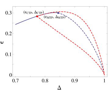
Figure 5: The most interesting region of the $(\Delta,\epsilon)$ phase diagram for the canonical and microcanonical ensembles at $K=1$. The solid blue line denotes second order transitions and ends at the CTP and the MTP for the canonical and microcanonical ensembles, respectively. Red (blue) dashed lines are the first order transition lines for the canonical (microcanonical) ensemble. The coordinates of the tricritical points are $\Delta_{CTP}\backsimeq 0.7726$, $\epsilon_{CTP}\backsimeq 0.2836$ and $\Delta_{MTP}\backsimeq 0.8439$, $\epsilon_{MTP}\backsimeq 0.2996$. The region inside the two red dashed lines is forbidden in the canonical ensemble. The first order lines meet at the point with coordinates $\Delta=1$ and $\epsilon=0$ (the minimum allowed energy for $\Delta=1$).

For convenience, we summarize the coordinates of the tricritical points for $K=1$.

$\bullet$ Canonical Tricritical Point: $T_{CTP}=0.6$, $\Delta_{CTP}\backsimeq 0.7726$, $\epsilon_{CTP}\backsimeq 0.2836$.

$\bullet$ Microcanonical Tricritical Point: $T_{MTP}\backsimeq 0.5078$, $\Delta_{MTP}\backsimeq 0.8439$, $\epsilon_{MTP}\backsimeq 0.2996$.

IV.2 Low-Intermediate values of $K$: $2.775\backsimeq K_{1}<K<K_{2}=3$

In this range of $K$ the phase diagram of the system becomes more complex, and ensemble inequivalence is characterized by more features. In fact, not only are the tricritical points and the first order transitions different in the two ensembles, but a critical and a triple point appear in the canonical ensemble, with no counterparts in the microcanonical ensemble. This is visualized in Fig. 6, that shows the $(\Delta,T)$ phase diagram for $K=2.85$; this value has been chosen as representative of this range.

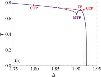
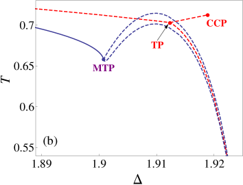
Figure 6: $(\Delta,T)$ phase diagram of the canonical and microcanonical ensembles at $K=2.85$: panel (a) shows the most interesting region, which is further zoomed in panel (b). The solid blue line denotes the line of second order transitions, ending at the CTP and the MTP for the canonical and microcanonical ensembles, respectively. Red (blue) dashed lines are the first order transition lines for the canonical (microcanonical) ensemble. The first order canonical line branches at the canonical triple point (TP): one branch reaches $T=0$ where it meets the two microcanonical first order lines at $\Delta=(K+1)/2=1.925$; the other branch ends at the canonical critical point (CCP). The coordinates of the relevant points, CTP, MTP, TP and CCP, are given in the text.

As before, at the canonical tricritical point (CTP) the canonical transition changes from second order to first order (the red dashed line), while the microcanonical transition remains second order up to the microcanonical tricritical point (MTP), from which the two blue dashed lines denote the two temperature branches associated to the microcanonical first order transition. However, now the first order canonical line branches in two lines at the triple point (TP): one branch extends to $T=0$, while the other ends at a canonical critical point (CCP). The canonical first order transitions corresponding to the branch going from the triple point to the critical point are transitions between paramagnetic states ($m=0$) with different values of the quadrupole moment $q$. Some details on the computation of the canonical critical point are given in Appendix A.

On the other hand, the structure of the microcanonical phase diagram is the same as that in the previous range of $K$. In fact, only a tricritical point is present, and there is no counterpart, in the microcanonical ensemble, of the canonical transition between different paramagnetic states. This is clearly seen in Fig. 6(b).

The caloric curves give a better image of what happens. They are shown in Fig. 7 for four different values of $\Delta$. As for Fig. 4, the red horizontal lines denote the portion of the canonical curves in the inequivalence range. Fig. 7(a) corresponds to a value of $\Delta$ which is larger than that of the microcanonical tricritical point and smaller than that of the canonical triple point; in this case there is a first order transition between a ferromagnetic state and a paramagnetic state in both ensembles; the transition is accompanied by a region of negative specific heat in the microcanonical ensemble.

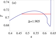
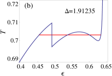
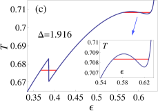
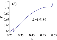
Figure 7: Caloric curves for $K=2.85$ and different values of the single-spin energy parameter $\Delta$. The meaning of the lines is the same as in Fig. 4.

For a value of $\Delta$ larger than that of the triple point, as in Fig. 7(c), the canonical caloric curve shows two first order transitions, the first (by increasing energy) from a ferromagnetic state to a paramagnetic state and the second between two paramagnetic states. As shown in the plot, in correspondence to this second canonical transition, the microcanonical ensemble presents only a region with negative specific heat, and no transition. This agrees with the fact that in Fig. 6 there is no line of microcanonical transitions associated to the canonical line going from the triple point to the critical point. At exactly the triple point (Fig. 7(b)) the two first order canonical transitions merge in a single one. Instead, by increasing $\Delta$ up to the critical point value, as in Fig. 7(d), the second canonical transition becomes continuous, and the caloric curve has a vanishing derivative at the transition point (infinite specific heat).

The phase diagram in the $(\Delta,\epsilon)$ plane is shown in Fig. 8. It happens that the energy of the second order microcanonical transition, for values of $\Delta$ between those of the canonical and the microcanonical tricritical points, is very close to the upper energy of the canonical first order transition, so that the two corresponding lines in the phase diagram are very close. The region inside the dashed red lines is forbidden in the canonical ensemble. The canonical TP in the $(\Delta,T)$ diagram splits in three points of the $(\Delta,\epsilon)$ diagram, which represent the energies of the three phases that meet at this point.

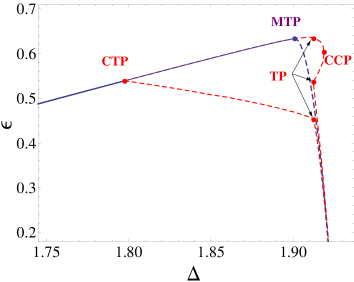
Figure 8: The most interesting region of the $(\Delta,\epsilon)$ phase diagram for the canonical and microcanonical ensembles at $K=2.85$. The blue solid line denotes the line of second order transitions, ending at CTP and MTP for the canonical and microcanonical ensembles, respectively. Red (blue) dashed lines are the first order transition lines for the canonical (microcanonical) ensemble. Between the CTP and the MTP the second order microcanonical line is extremely close (from below) to one of the first order canonical lines, so that in the plot they are practically indistinguishable. The plot shows the three energies of the canonical triple point (TP) and the canonical critical point (CCP). The first order lines meet at the point with coordinates $\Delta=1.925$ and $\epsilon=0$ (the minimum allowed energy for $\Delta=1.925$). The region inside the red dashed lines is forbidden in the canonical ensemble.

The coordinates of the relevant points of the phase diagrams for $K=2.85$ are:

$\bullet$ Canonical Tricritical Point: $T_{CTP}\backsimeq 0.7701$, $\Delta_{CTP}\backsimeq 1.7976$, $\epsilon_{CTP}\backsimeq 0.5392$,

$\bullet$ Canonical Triple Point: $T_{TP}=0.7030$, $\Delta_{TP}=1.91235$, $\epsilon_{TP}\backsimeq 0.4531;0.5367;0.6342$,

$\bullet$ Canonical Critical Point: $T_{CCP}=0.7125$, $\Delta_{CCP}\backsimeq 1.9189$, $\epsilon_{CCP}\backsimeq 0.6032$,

$\bullet$ Microcanonical Tricritical Point: $T_{MTP}\backsimeq 0.6581$, $\Delta_{MTP}\backsimeq 1.9008$, $\epsilon_{MTP}\backsimeq 0.6337$.

IV.3 Intermediate-High values of $K$: $3=K_{2}<K<K_{3}\backsimeq 3.801$

In this range of $K$ we have a new structure of the phase diagram. While the canonical structure is similar to that of the previous $K$ range, the microcanonical structure is characterized by the disappearance of the tricritical point and the appearance of a branching point, as explained in detail below, and a critical point. The representative value of $K$ that we have chosen for this range is $K=3.6$. In Fig. 9 we show both the $(\Delta,T)$ and the $(\Delta,\epsilon)$ phase diagrams. We notice that, although the structure of the canonical diagram

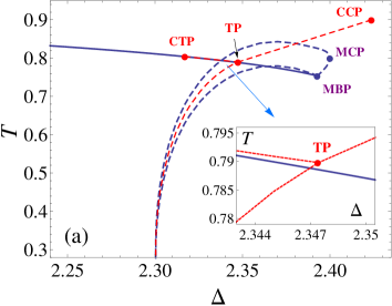
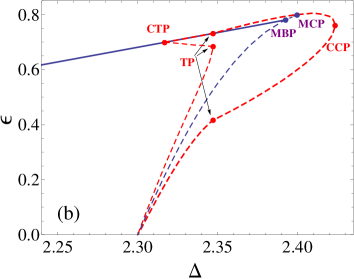
Figure 9: The most interesting region of the phase diagrams of the canonical and microcanonical ensembles at $K=3.6$. The solid blue line denotes the line of second order transitions, ending at the canonical tricritical point (CTP) and at a microcanonical branching point (MBP) for the two ensembles, respectively. Red (blue) dashed lines are the first order transition lines for the canonical (microcanonical) ensemble. (a) $(\Delta,T)$ phase diagram. Between the CTP and the triple point (TP) the first order canonical line is very close to the second order microcanonical line; the inset shows a zoom of the region near the TP. One canonical first order branch and the two microcanonical first order branches meet at $T=0$ at $\Delta=(K+1)/2=2.3$. (b) $(\Delta,\epsilon)$ phase diagram. The three energies of the canonical triple point (TP) are indicated. The first order lines meet at the point with coordinates $\Delta=2.3$ and $\epsilon=0$ (the minimum allowed energy for $\Delta=2.3$). The coordinates of the relevant points, CTP, MBP, MCP, TP and CCP, are given in the text.

is the same as before, now the $\Delta$ value where the transition lines meet the $T=0$ axis is smaller than that of the relevant points. On the other hand, the structure of the microcanonical diagram has completely changed. The microcanonical tricritical point is no more present. The reason is that the line of second order transition ends before the quantity $B_{m}$ of Eq. (26) reaches the value $0$: for $\Delta$ values larger than those where the line ends, the states corresponding to the critical line do not realize the absolute maximum of the microcanonical entropy and become metastable. Then, the critical line branches, at the microcanonical branching point (MBP), in two lines of first order transitions. We are denoting by MBP a point that in the literature is usually called microcanonical critical end point; see also the last Subsection. In the $(\Delta,T)$ diagram the lines departing from the MBP are those of the lower temperature associated to the temperature jump corresponding to the first order transition. For $\Delta$ values smaller than that of the MBP the transition is between a ferromagnetic and a paramagnetic state, while for $\Delta$ values larger than that of the MBP it is between two paramagnetic states . The line of first order transitions between paramagnetic states ends at the microcanonical critical point (MCP). In Appendix B we give some details on the computation of the microcanonical critical point. The inset in Fig. 9(a) shows the region near the canonical triple point, where the first order canonical line is very close to the second order microcanonical line. In the $(\Delta,\epsilon)$ diagram (panel (b) of the figure) one canonical first order branch and the microcanonical second order line are still closer, and a large magnification would be needed to reveal the gap between them.

In Fig. 10 we show the caloric curves at four different values of $\Delta$.

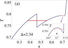
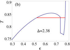
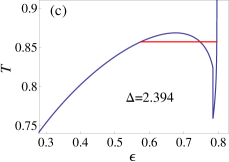
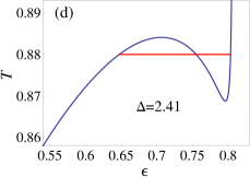
Figure 10: Caloric curves for $K=3.6$ and different values of the single-spin energy parameter $\Delta$. The meaning of the lines is the same as in Fig. 4.

Fig. 10(a) refers to a $\Delta$ value between the canonical tricritical point and the canonical triple point. Interestingly, by increasing the temperature or the energy the system goes from a paramagnetic to a ferromagnetic state and then back to a paramagnetic state. The first transition is first order in both ensembles, while the second transition is first order in the canonical ensemble and second order in the microcanonical ensemble, accompanied by a region of negative specific heat (it would be second order in both ensembles for a $\Delta$ value smaller than that of the CTP). For a $\Delta$ value between the CTP and the MBP (Fig. 10(b)) there is, in the canonical ensemble, only a first order transition between two paramagnetic states; in the microcanonical ensemble the situation is as in the previous plot, although now the negative specific heat occurs also before the temperature jump. For a $\Delta$ value between the MBP and the MCP (Fig. 10(c)) there is, in both ensemble, only a first order transition between two paramagnetic states. Finally, for $\Delta$ between the microcanonical and the canonical critical point (Fig. 10(d)) only the canonical transition is present, while the microcanonical ensemble shows just a region of negative specific heat. We will discuss in the Conclusions the analogy between this behaviour and the so-called gravitational phase transitions.

The coordinates of the relevant points of the phase diagrams for $K=3.6$ are:

$\bullet$ Canonical Tricritical Point: $T_{CTP}\backsimeq 0.8039$, $\Delta_{CTP}\backsimeq 2.3170$, $\epsilon_{CTP}\backsimeq 0.6994$,

$\bullet$ Canonical Critical Point: $T_{CCP}=0.9$, $\Delta_{CCP}\backsimeq 2.4238$, $\epsilon_{CCP}\backsimeq 0.7619$,

$\bullet$ Canonical Triple Point: $T_{TP}\backsimeq 0.7898$, $\Delta_{TP}\backsimeq 2.3474$, $\epsilon_{TP}\backsimeq 0.4168;0.6848;0.7321$,

$\bullet$ Microcanonical Branching Point: $T_{MBP}\backsimeq 0.7537$, $\Delta_{MBP}\backsimeq 2.3927$, $\epsilon_{MBP}\backsimeq 0.7809$,

$\bullet$ Microcanonical Critical Point: $T_{MCP}=0.8$, $\Delta_{MCP}=2.4$, $\epsilon_{MCP}=0.8$.

IV.4 High values of $K$: $K>K_{3}\backsimeq 3.801$

For large $K$ values we have yet another kind of structure of the phase diagram. We have chosen the value $K=5$ as representative for this case. In Fig. 11 we show both the $(\Delta,T)$ and the $(\Delta,\epsilon)$ phase diagrams.

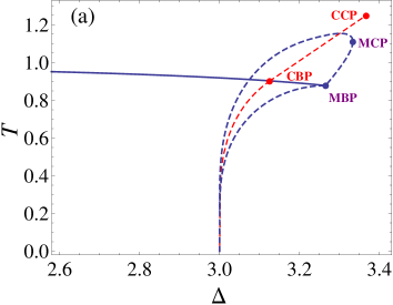
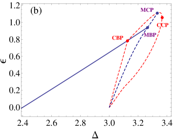
Figure 11: The most interesting region of the phase diagrams of the canonical and microcanonical ensembles at $K=5$. The solid blue line denotes the line of second order transitions, ending at the canonical branching point (CBP) and at a microcanonical branching point (MBP) for the two ensembles, respectively. Red (blue) dashed lines are the first order transition lines for the canonical (microcanonical) ensemble. (a) $(\Delta,T)$ phase diagram. One canonical first order branch and the two microcanonical first order branches meet at $T=0$ at $\Delta=(K+1)/2=3$. (b) $(\Delta,\epsilon)$ phase diagram. The first order lines meet at the point with coordinates $\Delta=3$ and $\epsilon=0$ (the minimum allowed energy for $\Delta=3$). The coordinates of the relevant points, CBP, MBP, MCP and CCP, are given in the text.

Now also the canonical ensemble does not present the tricritical point anymore. Analogously to what happens for the microcanonical ensemble in the previous $K$ range and also in this range, the line of canonical second order transition ends before the quantity $B_{c}$ of Eq. (12) reaches the value $0$. That is because the states corresponding to the critical line become metastable for values of $\Delta$ larger than those where the canonical critical line ends. It branches, at the canonical branching point (CBP), in two lines of first order transition (in the $(\Delta,\epsilon)$ diagram the lines departing from the CBP are those of the higher energy associated to the energy gap corresponding to the first order transition). As for the microcanonical case, for $\Delta$ values smaller than that of the CBP the transition is between a ferromagnetic and a paramagnetic state, while for $\Delta$ values larger than that of CBP it is between two paramagnetic states (in the literature the CBP is usually called canonical critical end point; see also the last Subsection). The line of first order transitions between paramagnetic states ends at the canonical critical point (CCP).

In Fig. 12 we show the caloric curves at four different values of $\Delta$.

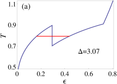
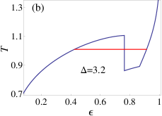
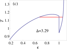
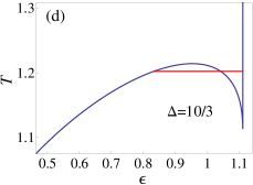
Figure 12: Caloric curves for $K=5$ and different values of the single-spin energy parameter $\Delta$. The meaning of the lines is the same as in Fig. 4.

Fig. 12(a) refers to a $\Delta$ value smaller than the canonical branching point, but larger than that where the first order lines meet the $T=0$ (or $\epsilon=0$) line. By increasing the temperature or the energy, the system goes from a paramagnetic to a ferromagnetic state and then back to an paramagnetic state. The first transition is first order in both ensembles, while the second transition is second order and coincides in both ensembles. For a $\Delta$ value between the canonical and the microcanonical branching points (Fig. 12(b)) there is, in the canonical ensemble, only a first order transition between two paramagnetic states; in the microcanonical ensemble there is a first order transition between the paramagnetic and the ferromagnetic state and then a second order transition between the ferromagnetic and the other paramagnetic state. For a $\Delta$ value between the MBP and the MCP (Fig. 12(c)) there is, in both ensembles, a first order transition between two paramagnetic states, with a region of negative specific heat before the microcanonical transition. Finally, at exactly the microcanonical critical point (Fig. 12(d)) the canonical first order transition is accompanied, in the microcanonical ensemble, by a second order transition, preceded by a region of negative specific heat.

The coordinates of the relevant points of the phase diagrams for $K=5$ are:

$\bullet$ Canonical Branching Point: $T_{CBP}\backsimeq 0.9031$, $\Delta_{CBP}\backsimeq 3.1256$, $\epsilon_{CBP}\backsimeq 0.7839$,

$\bullet$ Canonical Critical Point: $T_{CCP}=1.25$, $\Delta_{CCP}\backsimeq 3.3664$, $\epsilon_{CCP}\backsimeq 1.0582$,

$\bullet$ Microcanonical Branching Point: $T_{MBP}\backsimeq 0.8781$, $\Delta_{MBP}\backsimeq 3.2651$, $\epsilon_{MBP}\backsimeq 0.9395$,

$\bullet$ Microcanonical Critical Point: $T_{MCP}=10/9$, $\Delta_{MCP}=10/3$, $\epsilon_{MCP}=10/9$.

IV.5 Negative temperatures

We have already noticed that this system can achieve negative temperatures TGBtemp , since the energy is upper bounded. In this Subsection we evaluate which is the energy range in which the temperature is negative. Talking about negative temperatures, their physical meaning must be clearly kept in mind. In the microcanonical ensemble, they are a consequence of a negative derivative of the entropy with respect to the energy at the fixed energy at which the isolated system is considered, this negative derivative in turn being a consequence of the existence of an energy upper bound. Obviously, in the canonical ensemble a heat bath cannot have a negative temperature, forbidding a physical discussion of ensemble inequivalence. However, one could formally define a negative $\beta$, since the compact support of the phase space and the existence of an upper bound in energy give a finite partition function.

First of all, once we accept the formal definition of negative $\beta$, we can see that for negative temperatures the ensembles are equivalent. This could be determined with a complete analysis through calculations similar to those of Secs. II and III. For the canonical case we would arrive at an expression for $\tilde{f}(\beta,x,y)$ different from Eq. (6), since for negative $\beta$ the imaginary unit would appear in the second term of the exponent of the Hubbard-Stratonovich transformation (3). However, we prefer, for brevity, to resort to a heuristic argument.

We have seen that, for large enough positive $T$, the system, for any $\Delta$ and $K$, is in a paramagnetic state ($m=0$) and no further phase transition occurs. We know that, when there are no transitions in the canonical ensemble, the ensembles are equivalent, therefore we immediately conclude in favour of ensemble equivalence for negative temperatures, since by definition these temperatures are “hotter” than any positive temperature, favouring higher energy with respect to lower energy states. In particular, $T=-\infty$ coincides with $T=+\infty$, and by going from $T=-\infty$ to $T=0^{-}$ we progressively go to “hotter” and “hotter” temperatures, while energy will increase (positive specific heat) up to the upper bound foot4 . This is sufficient to determine the energy range where negative temperatures are realized. We just need to compute which is the energy of the system when $T=\infty$; between this value and the upper bound of the energy, temperatures will be negative.

For $T=\infty$ we have $m=0$ and $q=2/3$, since the three spin states are equally populated. Then the energy per particle will be (from, e.g., Eq. (17)) $\epsilon_{T=\infty}=\frac{2}{3}\Delta-\frac{2}{9}K$. The upper bound of the energy can be deduced as a consequence of the more detailed calculations in Sec. V and Appendix C for the bounds of the energy as a function of $m$. This energy upper bound is $\epsilon_{\rm max}=\frac{\Delta^{2}}{2K}$ for $\Delta/K\leq 1$, realized for $m=0$ and $q=\Delta/K$, and $\epsilon_{\rm max}=\Delta-\frac{K}{2}$ for $\Delta/K\geq 1$, realized for $m=0$ and $q=1$. It is straightforward to see that it is always $\epsilon_{\rm max}>\epsilon_{T=\infty}$, except for $\Delta/K=2/3$, when the two quantities are equal. Only in this last case, negative temperatures are not realized. This has a consequence on the determination of the microcanonical critical point (MCP), as shown in Appendix B.

IV.6 Analysis of the phase diagrams

The phase diagrams in the various $K$ ranges show different features. They can be analyzed in the framework of the classification of phase transitions given in Ref. bouchet05 . We do this here very briefly.

The phase transitions of a system, both in the microcanonical and in the canonical ensemble, can be deduced from the structure of the function $s(\epsilon)$ computed in the microcanonical ensemble, more precisely from its singularities. In turn, the singularities can be classified according to their codimension, to be defined below. Let us apply this concept to our system. We see from Eq. (19) that the function $S/N$ depends on the two order parameters $m$ and $q$, while Eq. (20) gives a relation between $m$, $q$, the energy $\epsilon$ and the two parameters of the Hamiltonian $\Delta$ and $K$. Solving Eq. (20) with respect to $q$, allows us to write $S/N$ as a function of $m$, $\epsilon$, $\Delta$ and $K$, obtaining the two functions $\tilde{s}_{\pm}$ (since Eq. (20) has two solutions). The maximization with respect to $m$ gives the equilibrium entropy. In Sec. III we have indicated explicitly only the dependence of $\tilde{s}_{\pm}$ on $m$ and $\epsilon$, and the dependence of the equilibrium entropy $s$ only on $\epsilon$. However, now it is useful to indicate explicitly also the dependence of $s$ on the Hamiltanian parameters $\Delta$ and $K$: $s=s(\epsilon;\Delta,K)$. Thus, we have a dependence on the energy plus two parameters. Accordingly, the thermodynamics phase space will have three dimensions, corresponding to $(\epsilon,\Delta,K)$ or $(T,\Delta,K)$. In our presentation of the results we have chosen to give the phase diagrams in the $(\Delta,\epsilon)$ or $(\Delta,T)$ space at various fixed values of $K$, since this was convenient for the central argument of our paper, namely to show ensemble inequivalence and the different structures of the phase diagram in the two ensembles in all ranges of $K$. However, to follow the picture depicted in Ref. bouchet05 we have to consider the three dimensional phase diagram.

If $R$ is the number of parameters the entropy depends on, $2$ in our case, i.e. $\Delta$ and $K$, a singularity is said to be of codimension $n$ if it spans a hypersurface of dimension $R-n$ in the thermodynamic phase space. Since $R=2$, we can have singularities of codimension $0$, $1$ and $2$, spanning hypersurfaces of dimension $2$, $1$ and $0$, respectively, in the three-dimensional thermodynamic phase space. Therefore, all the first order and second order transitions lines in Figs. 1, 3, 5, 6, 8, 9 and 11 represent codimension $0$ singularities: they are lines in the two-dimensional plots, but they exist for given ranges of $K$, and therefore they are two-dimensional hypersurfaces in the three-dimensional phase space. Analogously, the singularities that appear as points in the various two-dimensional plots, but that exist for given ranges of $K$, like the tricritical, critical, branching and triple points are codimension $1$ singularities. On the other hand, codimension $2$ singularities are not visible in our plots. They occur in isolated points in the three-dimensional phase space, exactly for the values of $K$ where the structure of the phase diagram changes; these are the boundaries of the $K$ ranges that we have indicated in the titles of the previous Subsections.

Singularities in the function $s(\epsilon;\Delta,K)$ can originate from different mechanisms, and we now present briefly their origin. The reader interested in the complete general theory finds full details in Ref. bouchet05 . Let us begin with the microcanonical first order transitions, associated to codimension $0$ singularities. They arise from the process of maximization of $\tilde{s}_{\pm}(\epsilon,m;\Delta,K)$ with respect to $m$ to get $s(\epsilon;\Delta,K)$. When the functions $\tilde{s}_{\pm}$ have more than one local maximum, one of which is the absolute maximum, the singularities, i.e. the first order transitions, occur when one local maximum becomes, changing $\epsilon$ or the parameters, the global one. This singularity spans a two dimensional hypersurface since it is defined by one condition, i.e. the equality of two maxima. This transition is always associated with a negative temperature jump (by increasing energy), as can be understood by the following. The inverse temperature $\beta$ is given by $(\partial s)/(\partial\epsilon)$, which is also equal to $(\partial\tilde{s}_{+})/(\partial\epsilon)$ or $(\partial\tilde{s}_{-})/(\partial\epsilon)$ (the one giving the global maximum) taken at the equilibrium magnetization. At the point of transition, when one local maximum becomes global, necessarily this must have a rate of increase with $\epsilon$ faster than the maximum becoming local from global; this means that the new maximum has a larger $\beta$, i.e., a smaller $T$.

The canonical first order transitions are other codimension $0$ singularities, and they have another origin. They come from the construction of the concave envelope of a function $s$ that has convex portions as a function of $\epsilon$. Also in this case there is only one condition, namely one has to locate the point in which the entropy $s$ is no more globally concave.

The final codimension $0$ singularity present in our model is represented by the critical line associated to second order transitions, either in both ensembles or only in the microcanonical ensemble. It can be shown bouchet05 that this kind of codimension $0$ singularity is present when there is a symmetry in the system, and the transition breaks the symmetry in the equilibrium state. In our case the symmetry is the $m\to-m$ invariance under change of sign, and the symmetry is between symmetric paramagnetic $m=0$ states that undergo a continuous transitions to states with $m\neq 0$ that break the symmetry. As explained in Appendix B in this case there is a jump in $(\mbox{d}\beta)/(\mbox{d}\epsilon)$, i.e. the caloric curve presents a discontinuity in the derivative. Now, the condition to satisfy is the vanishing of the second derivative of $\tilde{s}$ with respect to $m$ in $m=0$ for the microcanonical ensemble, and the vanishing of the second derivative of $\tilde{f}$ with respect to $x$ in $x=0$ for the canonical ensemble. As shown in Sec. III the latter condition is actually identical to the former.

We now consider codimension $1$ singularities, beginning from those due to the change of sign symmetry of the order parameter $m$. They are the tricritical points and the branching points in both ensembles. The two conditions giving the microcanonical tricritical point are the vanishing of the second and fourth order derivative of $\tilde{s}$ with respect to $m$ in $m=0$, while for the canonical tricritical point they are the vanishing of the second and fourth order variation of $\tilde{f}$ in $x=0$. It can be shown Campa09 that the vanishing of the fourth order variation of $\tilde{f}$ in $x=0$ is simply related to a condition on $\tilde{s}$ in $m=0$, confirming that the transitions in both ensembles are related to the structure of the microcanonical entropy.

We have already noticed that what we have called branching point is defined in the literature as critical end point. This is due to the fact that they are the intersection point of a critical line with a line of first order transitions. The critical line must end at the intersection point because the states related to the first order transitions are thermodynamically favoured; those associated to the critical line become metastable. The conditions giving rise to this situation are different in both ensembles, so the canonical and microcanonical branching points are located in different positions. For the microcanonical case, the point arises from the equality of three maxima with respect to $m$, two located on $\tilde{s}_{+}$ and one on $\tilde{s}_{-}$ (or viceversa). For the canonical case, it is defined by the appearance of a convex portion of $s$ at exactly the point of second order transition.

The remaining codimension $1$ singularities in our system are not associated to the change of sign symmetry. Let us begin with the canonical ensemble. The two conditions giving rise to the canonical critical point (Fig. 7(d)) are the vanishing at the same point of both the second and third order derivatives of $s$ with respect to $\epsilon$. On the other hand, the canonical triple point is related to the merging, in the function $s(\epsilon)$, of two regions not globally concave in a single one; this can be seen in Fig. 7, going from panel (c) to panel (b) (the triple point) and then to panel (a). We finally consider the microcanonical critical point. Normally, as explained in Appendix B, it is associated, in systems without symmetry, to the vanishing at the same point of the second and third order derivatives of $\tilde{s}$ with respect to $m$. But we have seen in the same Appendix that our system has a rather peculiar microcanonical critical point, located at the upper bound of the energy. In this case the two conditions are given by a relation between the two parameters, i.e., $\Delta=2K/3$, and the energy upper bound. This critical point is present when there is a line of first order transitions between two different paramagnetic states, and this occurs for $K>3$.

Codimension $2$ singularities are not explicitly treated in Ref. bouchet05 . As mentioned above, they are located at the $K$ values that mark the change of structure of the $(\Delta,T)$ or $(\Delta,\epsilon)$ phase diagram, i.e. at the point we have indicated with $K_{1}\backsimeq 2.775$, $K_{2}=3$ and $K_{3}\backsimeq 3.801$. At $K_{1}$ we have the appearance of the canonical triple point and the canonical critical point. The three conditions in this case are that the canonical critical point (two conditions) appears at the same point of the canonical first order transition (the other condition). It is as if the panels (b) and (d) of Fig. 7 would merge. At $K_{2}$ we have the disappearance of the microcanonical tricritical point and the appearance of the microcanonical branching and critical points. The three conditions defining this point are that the microcanonical tricritical point (two conditions) occurs at the upper bound of the energy (the other condition). Finally, at $K_{3}$ we have the disappearance of the canonical tricritical point and triple point and the appearance of the canonical branching point. This is due to the fact that the canonical tricritical point (two conditions) reaches the canonical first order transition line (the other condition) between the two paramagnetic states.

V Ergodicity breaking

Now, let us turn our attention to another interesting property of this system. That is ergodicity breaking in the microcanonical dynamics with fixed energy Borgonovi ; Schreiber . This statement assumes that the dynamics of the system, whose Hamiltonian has only discrete spin variables, is defined in such a way that, as in systems with continuous dynamical variables, thermodynamic parameters can vary only continuously. A microcanonical dynamics for spin systems, in which at each step only one spin is updated, has been introduced by Creutz creutz . Then, in the thermodynamic limit, magnetization $m$ can vary only continuously.

Ergodicity breaking at thermodynamic limit naturally occurs in nonadditive systems, like our mean-field model, where the absence of phase separation makes it possible to have a nonconvex region delimitating the accessible values of thermodynamic parameters. In this case breaking of ergodicity manifests itself by the presence of disjoint ranges of magnetization $m$ for a given energy value $\epsilon$. Therefore, a dynamics starting in one of the disjoint ranges cannot access states belonging to the other ranges, although these would be allowed energetically.

To see how this situation arises, we can adopt the following strategy. For a given value of the magnetization $m$, we look for the minimum and maximum values that can be achieved by the energy $\epsilon$; this will also determine, for a given energy $\epsilon$, which are the possible values of $m$.

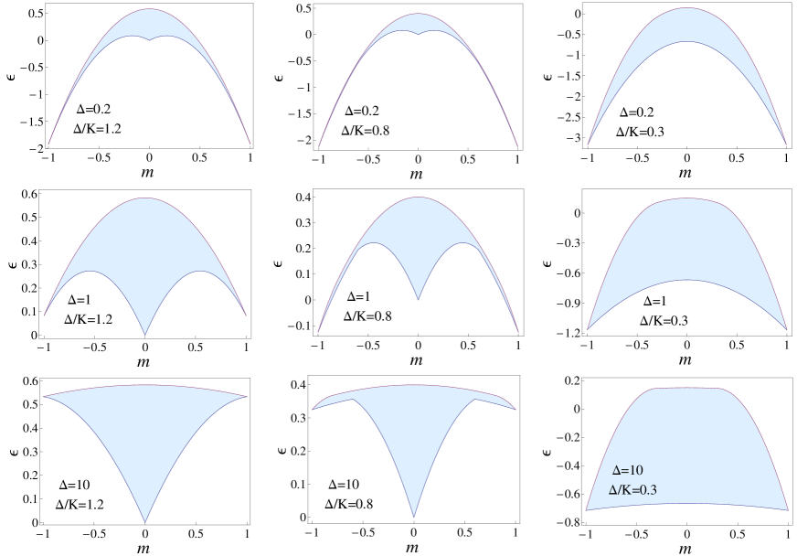
Figure 13: A schematic representation of the accessible region in the $m-\epsilon$ plane for fixed values of $\Delta$ and $\Delta/K$.

Let us rewrite Eq. (20) as

$$\epsilon=\Delta q-\frac{K}{2}q^{2}-\frac{m^{2}}{2}\,.$$ (30)

Magnetization $m$ varies in the range $-1\leq m\leq 1$, but by symmetry we can restrict the analysis to the range $0\leq m\leq 1$. As mentioned above, we are interested in the range of variability of energy $\epsilon$ for any given fixed value of $m$; in particular, we want to determine the minimum and maximum values of $\epsilon$ for any given value of $m$. We first notice that for a given $m$, the quantity $q$ varies in the range $m\leq q\leq 1$; therefore we have to determine, for any given $m$, the minimum and maximum values of $\epsilon$ given by Eq. (30) when $q$ varies in the range $m\leq q\leq 1$. We denote these values as $\epsilon_{\rm min}(m)$ and $\epsilon_{\rm max}(m)$, respectively. Detailed calculations are shown in Appendix C.

The functions $\epsilon_{\rm min}(m)$ and $\epsilon_{\rm max}(m)$ depend on the ratio $\Delta/K$. They are the following.

Case $\frac{\Delta}{K}\geq 1$

$$\epsilon_{\rm min}(m) = \Delta m-\frac{K}{2}m^{2}-\frac{m^{2}}{2}\,\,\,\,\,\,\,\,\,\,\,\,\,\,\,\,\,\,\,\,\,\,\,\,\,\,\,\,\,\,\,\,\,\,0\leq m\leq 1$$

$$\epsilon_{\rm max}(m) = \Delta-\frac{K}{2}-\frac{m^{2}}{2}\,\,\,\,\,\,\,\,\,\,\,\,\,\,\,\,\,\,\,\,\,\,\,\,\,\,\,\,\,\,\,\,\,\,\,\,\,\,\,\,\,\,\,\,\,\,\,0\leq m\leq 1$$

Case $\frac{1}{2}\leq\frac{\Delta}{K}\leq 1$

$$\epsilon_{\rm min}(m) = \Delta m-\frac{K}{2}m^{2}-\frac{m^{2}}{2}\,\,\,\,\,\,\,\,\,\,\,\,\,\,\,\,\,\,\,\,\,0\leq m\leq\frac{2\Delta}{K}-1$$

$$\epsilon_{\rm min}(m) = \Delta-\frac{K}{2}-\frac{m^{2}}{2}\,\,\,\,\,\,\,\,\,\,\,\,\,\,\,\,\,\,\,\,\,\,\,\,\,\,\,\,\,\,\,\,\,\,\frac{2\Delta}{K}-1\leq m\leq 1$$

$$\epsilon_{\rm max}(m) = \frac{\Delta^{2}}{2K}-\frac{m^{2}}{2}\,\,\,\,\,\,\,\,\,\,\,\,\,\,\,\,\,\,\,\,\,\,\,\,\,\,\,\,\,\,\,\,\,\,\,\,\,\,\,\,\,\,\,\,0\leq m\leq\frac{\Delta}{K}$$

$$\epsilon_{\rm max}(m) = \Delta m-\frac{K}{2}m^{2}-\frac{m^{2}}{2}\,\,\,\,\,\,\,\,\,\,\,\,\,\,\,\,\,\,\,\,\,\,\frac{\Delta}{K}\leq m\leq 1$$

Case $0\leq\frac{\Delta}{K}\leq\frac{1}{2}$

$$\epsilon_{\rm min}(m) = \Delta-\frac{K}{2}-\frac{m^{2}}{2}\,\,\,\,\,\,\,\,\,\,\,\,\,\,\,\,\,\,\,\,\,\,\,\,\,\,\,\,\,\,\,\,\,\,\,\,\,\,0\leq m\leq 1$$

$$\epsilon_{\rm max}(m) = \frac{\Delta^{2}}{2K}-\frac{m^{2}}{2}\,\,\,\,\,\,\,\,\,\,\,\,\,\,\,\,\,\,\,\,\,\,\,\,\,\,\,\,\,\,\,\,\,\,\,\,\,\,\,\,\,\,\,\,\,\,\,0\leq m\leq\frac{\Delta}{K}$$

$$\epsilon_{\rm max}(m) = \Delta m-\frac{K}{2}m^{2}-\frac{m^{2}}{2}\,\,\,\,\,\,\,\,\,\,\,\,\,\,\,\,\,\,\,\,\,\,\,\,\frac{\Delta}{K}\leq m\leq 1$$

The functions $\epsilon_{\rm min}(m)$ and $\epsilon_{\rm max}(m)$ are always continuous. Also their derivatives are continuous, except the derivative of $\epsilon_{\rm min}(m)$ in the case $\frac{1}{2}\leq\frac{\Delta}{K}\leq 1$, which has a discontinuity at $m=\frac{2\Delta}{K}-1$. The results are extended by symmetry to negative values of $m$. In Fig. 13 we report an example for each one of the three cases.

The structure of the plots determines if an ergodicity breaking is present and in which way it is realized. We observe in the plots that, although the functional form of $\epsilon_{\rm min}(m)$ and $\epsilon_{\rm max}(m)$ depends only on the ratio $\Delta/K$, some relevant features depend on both $\Delta/K$ and $\Delta$. For example, from the above results, we obtain that the upper bound of the energy is always realized for $m=0$, and its value depends only on the ratio $\Delta/K$, being equal to $\Delta^{2}/(2K)$ for $\Delta/K\leq 1$ and equal to $\Delta-K/2$ for $\Delta/K\geq 1$. On the other hand, for $\Delta/K\leq 1/2$ the minimum possible value of the energy is always realized for $m=1$, and it is equal to $\Delta-(K+1)/2<0$; while for $\Delta/K\geq 1/2$ this occurs only when $\Delta-(K+1)/2<0$ (this condition being always realized when $\Delta/K<1/2$), otherwise the minimum is obtained for $m=0$ and it is equal to $0$. We remark that this result on the minimum energy is consistent with the first order transition at $T=0$ between a fully magnetized ferromagnetic state and a paramagnetic state at $\Delta=(K+1)/2$ (see Sec. II).

These results show that, when $\Delta/K<1/2$, ergodicity breaking is due to the fact that, for some values of the energy $\epsilon$, magnetization $m$ can achieve values in two disjoint ranges $m_{1}\leq m\leq m_{2}$ and $-m_{2}\leq m\leq-m_{1}$, with $0<m_{1}<m_{2}$. When $\Delta/K>1/2$ one can have this situation, but also a more complex situation in which magnetization can take values in three disjoint ranges, $-m_{2}\leq m\leq-m_{1}$, $-m_{0}\leq m\leq m_{0}$ and $m_{1}\leq m\leq m_{2}$, with $0<m_{0}<m_{1}<m_{2}$. It is also possible, for $\Delta/K>1$, to fall into a case in which ergodicity breaking is absent, as in the plot in the left bottom panel of Fig. 13; it is not difficult to compute that this occurs, for a given ratio $\Delta/K=r>1$, when $\Delta>r/(r-1)$.

VI Conclusions

The Blume-Emery-Griffiths (BEG) model was completely solved in the mean-field approximation in the canonical ensemble Blume71 . The study has been extended to the case where the Hamiltonian was augmented with an external magnetic field term mukamel74 , revealing the complexity of the canonical phase diagram. The microcanonical solution of the Blume-Capel model Blume66 , a simplified version of the BEG model, was first obtained in Ref. Barre01 and ensemble inequivalence was discussed in this context.

In this paper, we have extended the microcanonical solution to the original BEG model, showing a wealth of different features in the phase diagrams pertaining to the canonical and microcanonical ensembles.

As we have remarked in Sec. IV.6, the phase diagram of the model should be represented in terms of three parameters $(\Delta,T,K)$ or $(\Delta,\epsilon,K)$, where $T$ is temperature and $\epsilon$ the energy density. However, for convenience we have fixed the value of the biquadratic interaction coefficient $K$ and represented the $(\Delta,T)$ and $(\Delta,\epsilon)$ phase diagrams. For different values of $K$ one observes various facets under which ensemble inequivalence occurs.

At small values of $K$, the behavior is the one observed for the Blume-Capel model and for other models: the two ensembles have a common critical line of continuous transitions, terminating at tricritical points that are distinct in both ensembles. In the region where the transition is first order in the canonical ensembles the phase transition lines do not coincide. In conclusion, whenever the transition is continuous in both ensembles they are equivalent, while they are not equivalent when the transition is first order in the canonical or in both.

This generally occurs when there is a symmetry of the entropy under a sign change of the order parameter ($m\to-m$) bouchet05 , as also displayed by an analysis of the neighborhood of the transition points through a Landau expansion ocohen .

For larger values of $K$, above a given threshold $K_{1}$ for canonical ensemble and $K_{2}$ for the microcanonical ensemble, the model has also a transition between different paramagnetic states ($m=0$). This additional transition is characterized by a change in the quadrupole moment $q$ and is not associated to a symmetry under change of sign of $q$. As we have seen, while a symmetry breaking second order canonical transition point is also a second order microcanonical transition point, this is no more the case when the transition is not associated to a symmetry breaking. Moreover, critical points in different ensembles do not necessarily coincide for non symmetry breaking transitions. This remark was already partly contained in Refs. bouchet ; ocohen .

The interest of the BEG model is that within the same simple model both situations occur, i.e. symmetry breaking and non symmetry breaking transitions. The latter type is the typical situations that occurs for self-gravitating systems campa2016 ; chavanis02 , namely, for a value of the control parameter ($\Delta$ in our case) intermediate between those pertaining to the canonical and the microcanonical critical points, the system has a first order transition in the canonical ensemble, while in the microcanonical ensemble it has a region of negative specific heat without singularities.

Although at first glance it might seem the contrary, the fact that the canonical critical point is a generic point of the phase diagram for the microcanonical ensemble does not spoil the general fact that when the canonical ensemble has a continuous transition the ensembles are equivalent Barre01 ; touch04 ; foot5 . In fact, at exactly the canonical critical point the canonical and microcanonical caloric curves are identical (see, e.g. Fig. 7(d)). Therefore, the thermodynamic functions and their derivatives of all orders with respect to the thermodynamic variables are identical in both ensembles, showing in particular a diverging specific heat at the transition temperature or energy. As a consequence of this divergence, as soon as the parameter $\Delta$ decreases from the critical value, the canonical ensemble shows a first order transition, while the microcanonical ensemble has a region of negative specific heat.

We have based our analysis on the study of the singularities of the microcanonical entropy function. In the literature this has been characterized as the thermodynamic level of ensemble inequivalence, and it has been compared to the macrostate level, based on the properties of the correspondence between the equilibrium states occurring in the two ensembles ellis04 ; touch04 ; ellis2000 . At the energies where the microcanonical entropy coincides with the Legendre-Fenchel transform of $\beta f(\beta)$, the ensembles are equivalent at the thermodynamic level, otherwise they are not equivalent at this level and also at the macrostate level. At the energies where equivalence at the thermodynamic level occurs, the ensemble can be, at the macrostate level, either fully equivalent or partially equivalent ellis2000 . According to this classification, in a case like ours, in which there are no ranges of energy where the microcanonical entropy is a straight line (due to the absence of phase separation), there is partial equivalence at the macrostate level only at the energies where a first order canonical phase transition occurs (thus there are no ranges of partial equivalence, but only isolated energy values); more specifically, the points of partial equivalence are those at the two extremes of each segment marking a Maxwell construction.

The study of the BEG model in the canonical ensemble has been performed in the past on a Bethe lattice anan91 ; anan96 . In this case, the model can be exactly solved using recursive relations for the partition function. Inequivalence for Bethe lattices was studied for the Potts model barre07 . Using the cavity technique applied in the latter paper, one could solve the BEG model on a Bethe lattice and analyze ensemble inequivalence. The Blume-Capel model on long-range random networks was recently studied in Ref. Levon . Inequivalence was shown to occur near first order phase transitions using extensive numerical simulations. A class of models sometimes considered is the one of equivalent-neighbor models. When the cutoff distance in this model is infinite they become identical to mean-field models, although for any large but finite cutoff distance their critical behavior is different from that of mean-field models lui1996 ; qian2016 . This should not be surprising, since a finite cutoff distance makes the interaction integrable, as in short-range systems.

Monte Carlo evaluations and renormalization group analyses have been performed in the past to investigate the BEG model with nearest-neighbor interaction (see, eg., Refs. wang1987 ; berker1976 ; hoston1991 ; netz1993 ). We note that these interesting and relevant studies concern models with short-range interactions, where it suffices to study the canonical ensemble, since ensemble equivalence occurs.

As noted in the introductory remarks, negative specific heat in the microcanonical ensemble was found in self-gravitating systems long time ago; then, an important review by Padmanabhan padma was dedicated almost three decades ago to the statistical mechanics of these systems (see also, e.g., Refs. padma89 ; chava02 ). In the study of self-gravitating systems, an important role is played by spherical shell models, used to investigate the consequences of the singularity that is present in Newtonian gravity. Model systems composed of irrotational or rotating concentric self-gravitating shells have been employed to study phase transitions in the different ensembles (see, e.g., Refs. miller98 ; klinko01 ). Ensemble inequivalence was found using mean-field theory, and confirmed with molecular dynamics simulations. Another important aspect is the role played by boundary conditions. Recently, it has been shown that in a onedimensional self-gravitating system in which periodic boundary conditions are imposed, a second order phase transition at finite temperature is present, contrary to what happens with free boundary conditions, where no transition is found kumar2017 . Also in this case the study was conducted using mean-field theory, and the results were confirmed with dynamical simulations.

Furthermore, we have considered the occurrence of ergodicity breaking by studying the structure of the accessible regions in the magnetization-energy phase space. Ergodicity breaking naturally occurs in non additive systems. We have seen that also for this feature the overall structure is strongly dependent on the relative values of $\Delta$ and $K$.

Concluding, we have shown that even a simple model like the BEG model can present many different singular points in the phase diagrams of the two ensembles and, correspondingly, ensemble inequivalence shows up in different ways. This confirms the usefulness of simple models as benchmarks for a detailed study of the possible physical situations that can arise in more complex and realistic non additive systems.

Appendix A The canonical critical line, tricritical point and isolated critical point

Following Landau theory, canonical second order phase transition points are characterized by the vanishing of the Hessian of $\tilde{f}$. These points satisfy Eqs. (8) and (9), that we rewrite here in the following form, using the common notation for partial derivatives

$$\tilde{f}_{x} = 0$$ (31)

$$\tilde{f}_{y} = 0.$$ (32)

We are interested in the solutions for which $x=0$, $y=1/\beta$, characterizing the transition between ferromagnetic and paramagnetic states. The vanishing of the Hessian is given by

$$\tilde{f}_{xx}\tilde{f}_{yy}-\tilde{f}_{xy}^{2}=0.$$ (33)

Since the critical point itself is an equilibrium point, $\tilde{f}$ must have a minimum at this point. On the other hand, the vanishing of the Hessian implies that there is a direction in the $(x,y)$ plane along which the second order variation of $\tilde{f}$ vanishes. This direction is exactly given by either one of the Eqs. (31) and (32). In our particular case $\tilde{f}$ is even in $x$, and thus $\tilde{f}_{xy}=0$ at $x=0$, and Eq. (33) implies that the critical points with $x=0$ are characterized by either $\tilde{f}_{xx}=0$ or $\tilde{f}_{yy}=0$ foot3 . The critical line corresponds to the case $\tilde{f}_{xx}=0$ (the case $\tilde{f}_{yy}=0$ will be treated below). The condition $\tilde{f}_{xx}=0$ is expressed by Eq. (11). In this case the direction of vanishing second order variation is the $x$ axis. We use Eq. (32) to define implicitly a function $y(x)$. The path in the $(x,y)$ plane defined by this function is tangent to the $x$ axis in $x=0$, since $y_{x}=-\tilde{f}_{xy}/\tilde{f}_{yy}$ (then $y_{x}=0$ at $x=0$), so that the tangent to this path in $x=0$ gives the direction of vanishing Hessian. Moreover, for any given fixed $x$ around $x=0$, $\tilde{f}_{y}=0$ gives the $y$ values for which $\tilde{f}$ is minimum. It is then clear that we now have to study the third order variation of $\tilde{f}$ as a function of $x$ when $y$ is the function of $x$ implicitly given by Eq. (32). Then, a straightforward calculation shows that the third order variation is given by $(\mbox{d}x)^{3}/6$ multiplied by the expression

$$\tilde{f}_{xxx}+3\tilde{f}_{xxy}y_{x}+3\tilde{f}_{xyy}y_{x}^{2}+\tilde{f}_{yyy}y_{x}^{3}+3\tilde{f}_{xy}y_{xx}$$ (34)

$$+ 3\tilde{f}_{yy}y_{x}y_{xx}+\tilde{f}_{y}y_{xxx},$$

computed at $x=0$. Since in our case $\tilde{f}$ is even in $x$, $\tilde{f}_{y}=0$ and $y_{x}=0$, then this expression vanishes. An analogous longer but again straightforward calculation gives the expression of the fourth order variation. Writing only the terms that do not vanish in $x=0$ we obtain the expression

$$\tilde{f}_{xxxx}+6\tilde{f}_{xxy}y_{xx}+3\tilde{f}_{yy}y_{xx}^{2}\,.$$ (35)

In this expression we substitute $y_{xx}$ as obtained by Eq. (32). Again keeping only the terms that do not vanish we get

$$\tilde{f}_{xxxx}-3\frac{\tilde{f}_{xxy}^{2}}{\tilde{f}_{yy}}.$$ (36)

The values of the terms of this expression at $x=0$, $y=1/\beta$ are easily computed, and we get the condition for the positiveness of the fourth order variation

$$\beta\frac{-\beta\left(1+2K\right)+\left(3+2K\right)}{\beta-K\beta+K}>0\,.$$ (37)

The numerator is exactly the expression in Eq. (12). It can be easily checked that, as a function of $\beta$, the denominator is positive when the numerator is positive, therefore the condition of positiveness is given by the numerator, and we thus get Eq. (12). When the numerator vanishes we obtain the tricritical point.

Eqs. (31) and (32) can admit other solutions with $x=0$ but $y\neq 1/\beta$, and it is possible to have transitions between paramagnetic states characterized by different values of the quadrupole moment $q$. A critical point is then obtained when this transition becomes continuous. Since these states have $x=0$, we can treat this problem as if we had the single order parameter $y$. The critical points are then characterized by

$$\tilde{f}_{y}=\tilde{f}_{yy}=\tilde{f}_{yyy}=0\,,$$ (38)

computed at $x=0$. There is no symmetry of $\tilde{f}$ as a function of $y$, and then the odd derivatives with respect to $y$ do not vanish identically. For a fixed $K$ value the three equations in (38) determine the values of $y$, $\beta$ and $\Delta$, and therefore there is a single critical point, at variance with the line of critical points obtained before. This difference is a consequence of the symmetry of $\tilde{f}$ with respect to $x$ bouchet05 . The solution of the three equations (38) is easily obtained

$$y=\frac{1}{2}\,\,\,\,\,\,\,\,\,\,\,\,\,\,\,\beta=\frac{4}{K}\,\,\,\,\,\,\,\,\,\,\,\,\,\,\,\Delta=\frac{K}{4}\left(2+\ln 2\right).$$ (39)

This solution holds for any $K>0$. However, since the former analysis is local, it does not determine if the point is a local or global minimum of $\tilde{f}$; only in the latter case the critical point actually exists. We have found that this happens only for $K$ larger than a threshold $K_{1}$, determined numerical to be about $2.775$.

In principle one could have a critical point in which Eq. (33) is satisfied with all three second derivatives $f_{xx}$, $f_{yy}$ and $f_{xy}$ different from $0$. This would imply the presence of transitions between different ferromagnetic states ($f_{xy}$ can be different from $0$ only for $x$ different from $0$). The associated isolated critical point would occur when this transition becomes continuous. However, this system does not present transitions between different ferromagnetic states, and therefore such a critical point does not occur.

Appendix B The microcanonical tricritical point and isolated critical point

The values of $\Delta$ and $T$ at the microcanonical tricritical point can be obtained by Eqs. (25), (26) and (28). The relation $B_{m}=0$, used together with $A_{m}=0$ and the definition of $T$ in Eq. (28), gives:

$$-\frac{3\beta}{\beta-1}+6(\beta\Delta-K)-2(\beta\Delta-K)^{2}+3K=0\,.$$ (40)

On the one hand, this equation can be solved for $\Delta$ as a function of $\beta$, by writing it in the form

$$2\beta^{2}(\beta-1)\Delta^{2}-2\beta(\beta-1)(3+2K)\Delta$$ (41)

$$+ 3\beta+(\beta-1)(2K^{2}+3K)=0\,,$$

whose solution in terms of $T=1/\beta$ is

$$\Delta_{MTP} = \frac{(2K+3)T_{MTP}}{2}$$

$$- \frac{\sqrt{3}T_{MTP}}{2}\sqrt{\frac{1-3T_{MTP}+2K(1-T_{MTP})}{1-T_{MTP}}}$$

(the relevant solution being the one giving the smaller value of $\Delta_{MTP}$). On the other hand, by using again Eq. (28) in the first term of Eq. (40) allows to write the latter equation as

$$-3\frac{e^{\beta\Delta-K}+2}{e^{\beta\Delta-K}}+6(\beta\Delta-K)-2(\beta\Delta-K)^{2}+3K=0\,.$$ (43)

Defining $w=\beta\Delta-K$ we then have an equation for $w$

$$2w^{2}-6w+6e^{-w}+3-3K=0\,.$$ (44)

Solving numerically this equation for $w$ one obtains $\beta_{MTP}\Delta_{MTP}$. Dividing both members of Eq. (B) by $T_{MTP}$ and plugging the obtained value in the left hand side one can obtain $T_{MTP}$, after which one gets $\Delta_{MTP}$ by $T_{MTP}(\beta_{MTP}\Delta_{MTP})=T_{MTP}(w+K)$.

As far as the dependence on order parameters is concerned, the functions $\tilde{s}_{\pm}(\epsilon,m)$ depend only on $m$, and they are even in this variable. The points of microcanonical continuous transition should then occur when the necessary condition $(\partial^{2}\tilde{s}_{\pm})/(\partial m^{2})=0$ is verified. However, this is not the case as we now explain, and, as we will see, it is possible to have an isolated critical point, at the end of a line of first order transitions, by another mechanism; however, this will be a rather peculiar critical point. To have a lighter notation, we neglect, in the following, the subscript $\pm$, denoting with $\tilde{s}(\epsilon,m)$ the function to be maximized with respect to $m$ to have $s(\epsilon)$; the argument does not depend on which of the functions $\tilde{s}_{\pm}$ realizes the absolute maximum.

Using, as in the previous Appendix, the common notation for partial derivatives, the equilibrium magnetization, as we know, is given by $\tilde{s}_{m}=0$ with $\tilde{s}_{mm}<0$. The former relation defines the function $m(\epsilon)$ at equilibrium, and from it we get

$$\frac{\mbox{d}m}{\mbox{d}\epsilon}=-\frac{\tilde{s}_{m\epsilon}}{\tilde{s}_{mm}}\,.$$ (45)

From this relation one obtains

$$\frac{\mbox{d}\beta}{\mbox{d}\epsilon}=\frac{\mbox{d}^{2}s}{\mbox{d}\epsilon^{2}}=\tilde{s}_{\epsilon\epsilon}-\frac{\tilde{s}_{m\epsilon}^{2}}{\tilde{s}_{mm}}\,.$$ (46)

This relation shows that the points of continuous transition, where $\beta(\epsilon)$ is continuous but $(\mbox{d}\beta)/(\mbox{d}\epsilon)$ has a singularity, are characterized by $\tilde{s}_{mm}=0$, with the further conditions $\tilde{s}_{mmm}=0$ and $\tilde{s}_{mmmm}<0$. The critical line in the $(\Delta,T)$ plane for the continuous transition between a ferromagnetic state and a paramagnetic state, evaluated in Sec. III, is included in this case, since we have obtained it from a power expansion of $\tilde{s}(\epsilon,m)$ at $m=0$, posing $A_{m}=\tilde{s}_{mm}/2=0$ and $B_{m}=\tilde{s}_{mmmm}/24<0$; the function $\tilde{s}(\epsilon,m)$ is even in $m$, so that $\tilde{s}_{mmm}$ identically vanishes in $m=0$. Since this implies that also $\tilde{s}_{m\epsilon}$ identically vanishes at $m=0$, the singularity of $(\mbox{d}\beta)/(\mbox{d}\epsilon)$ at the transition point is represented by a jump (except at the tricritical point, where this quantity diverges). On the other hand, if a continuous transition would occur at $m\neq 0$, where $\tilde{s}_{m\epsilon}\neq 0$ and $\tilde{s}_{mmm}$ does not vanish identically, one should explicitly require that $\tilde{s}_{mmm}=0$ at the point of continuous transition; this would then be the critical point at the end of a line a first order transitions, and it would have $(\mbox{d}\beta)/(\mbox{d}\epsilon)=+\infty$ ($\tilde{s}_{mm}$ tends to $0$ from below). However, as in the canonical ensemble, this system does not present transitions between different ferromagnetic states, and thus such a critical point does not occur.

Nevertheless, Eq. (46) shows that a singularity in $(\mbox{d}\beta)/(\mbox{d}\epsilon)$ can occur when there is a singularity in $\tilde{s}_{\epsilon\epsilon}$. The presence of this singularity is a consequence of the existence of an upper bound in the energy for our system. We start by computing the first and second derivatives of $\tilde{s}$ with respect to $\epsilon$; in doing so, we assume from the start that $m=0$, since we have to find the critical point of the transition between two paramagnetic states. Therefore we have:

$$\frac{\partial\tilde{s}_{\pm}}{\partial\epsilon} = \beta=\frac{\partial\tilde{s}_{\pm}}{\partial q}\frac{\partial q_{\pm}}{\partial\epsilon}$$ (47)

$$= \mp\frac{1}{K}\ln\left[\frac{2(1-q_{\pm})}{q_{\pm}}\right]\frac{1}{\sqrt{\left(\frac{\Delta}{K}\right)^{2}-\frac{2\epsilon}{K}}}\,,$$

and

$$\frac{\partial^{2}\tilde{s}_{\pm}}{\partial\epsilon^{2}} = \frac{\partial^{2}\tilde{s}_{\pm}}{\partial q^{2}}\left(\frac{\partial q_{\pm}}{\partial\epsilon}\right)^{2}+\frac{\partial\tilde{s}_{\pm}}{\partial q}\frac{\partial^{2}q_{\pm}}{\partial\epsilon^{2}}$$ (48)

$$= -\frac{1}{K^{2}q_{\pm}(1-q_{\pm})\left[\left(\frac{\Delta}{K}\right)^{2}-\frac{2\epsilon}{K}\right]}$$

$$\mp \frac{1}{K^{2}}\ln\left[\frac{2(1-q_{\pm})}{q_{\pm}}\right]\frac{1}{\left[\left(\frac{\Delta}{K}\right)^{2}-\frac{2\epsilon}{K}\right]^{\frac{3}{2}}}$$

where for convenience we rewrite the expression of $q_{\pm}$ for $m=0$:

$$q_{\pm}=\frac{\Delta}{K}\pm\sqrt{\left(\frac{\Delta}{K}\right)^{2}-\frac{2\epsilon}{K}}\,.$$ (49)

We are interested in the value of Eqs. (47) and (48) at the upper bound $\epsilon_{\rm max}$ of the energy. Let us begin with the case $\Delta/K\geq 1$. Obviously in this case $q_{+}$ is not acceptable, and we have to consider only $q_{-}$. When $\epsilon\to\epsilon_{\rm max}=\Delta-K/2$, then $q_{-}\to 1^{-}$. Thus, from Eq. (47) we see that $\beta\to-\infty$, and the upper bound of the energy coincides with $T=0^{-}$. Since the first derivative diverges, also the second does, but then this is not associated to a critical point; this point of the phase diagram does not mark the end of a line of first order transitions.

We now consider $\Delta/K<1$. We separate this analysis in three parts, corresponding to $\Delta/K<2/3$, $\Delta/K>2/3$ and $\Delta/K=2/3$. The reason is the following. For $\Delta/K<1$ the upper bound $\epsilon_{\rm max}=\Delta^{2}/(2K)$ is realized for $q=\Delta/K$, and the value $q=2/3$ is the one separating positive and negative values of the logarithm appearing in Eq. (47). We know that the entropy of the system will be given by the largest between $\tilde{s}_{+}$ and $\tilde{s}_{-}$. For $\Delta/K<2/3$ (respectively $>2/3$) and an energy sufficiently close to $\epsilon_{\rm max}$ also $q$ will be $<2/3$ (respectively $>2/3$). Since $(\partial\tilde{s})/(\partial q)=\ln\left[2(1-q)/q\right]$ is positive (respectively negative) for $q<2/3$ (respectively $>2/3$) we have to choose $q_{+}$, i.e. $\tilde{s}_{+}$ (respectively $q_{-}$, i.e. $\tilde{s}_{-}$) for $\Delta/K<2/3$ (respectively $\Delta/K>2/3$). Then we see from Eq. (47) that, for both $\Delta/K<2/3$ and $\Delta/K>2/3$, $\beta\to-\infty$ when $\epsilon\to\epsilon_{\rm max}$. As before, the first derivative diverges, and the divergence of the second derivative is not associated to a critical point.

On the other hand, for $\Delta/K=2/3$ the situation is different. For $q=2/3$, $(\partial\tilde{s})/(\partial q)=\ln\left[2(1-q)/q\right]=0$, so to determine the choice between $q_{+}$ and $q_{-}$ we have to compute higher derivatives of $\tilde{s}$ with respect to $q$. Without showing the calculations, we give the result that we have to choose $q_{-}$, i.e. $\tilde{s}_{-}$, so that, for $\epsilon\to\epsilon_{\rm max}$, $q\to\Delta/K=2/3$ from below. Then, from Eq. (47) we get that $\beta$ tends to a positive value; the important thing is that this value is finite. This can be obtained performing the limit, in which the argument of the logarithm tends to $1$ and the argument of the square root in the denominator tends to $0$. One gets that the limit of $\beta$ is equal to $9/(2K)$. Performing the same limit evaluation in Eq. (48) one finds that the second derivatives diverges to $+\infty$ (thus the derivative of $T$ with respect to $\epsilon$ diverges to $-\infty$). This is exactly the divergence giving rise to the critical point, that occurs at $\Delta=2K/3$, $T=2K/9$ and $\epsilon=2K/9$. This point is at the end of a line of first order transitions. In Fig. 12(d) we show the caloric curve for that value of $\Delta$ for $K=5$. Since the critical point has the peculiarity of occurring at exactly the upper bound of the energy, in that graph the temperature has a vertical jump to $T=+\infty$ at the same energy. This critical point can be present only when there is a line of microcanonical first order transitions between different paramagnetic states; as described in Sec. IV.6 this occurs for $K>K_{2}=3$. For $K<3$ the point of the microcanonical $(\Delta,T)$ phase diagram with coordinates $\Delta=2K/3$ and $T=2/3$, corresponding in the $(\Delta,\epsilon)$ diagram to $\epsilon=2K/9$, belongs to the critical line of second order transitions. In that case, a limiting procedure in Eq. (46), tedious but straightforward, shows that the caloric curve has a finite derivative for $\epsilon$ tending to the upper bound.

Appendix C The energy range as a function of the magnetization

Considering the right hand side of Eq. (30) as a function of $q$, it is a downward parabola with vertex in $q=\frac{\Delta}{K}$, then with positive derivative for $q<\frac{\Delta}{K}$ and negative derivative for $q>\frac{\Delta}{K}$. We are thus led to consider two main cases, i.e. $\frac{\Delta}{K}\geq 1$ and $\frac{\Delta}{K}\leq 1$, respectively.

In the first case the range $m\leq q\leq 1$ is entirely in the region of the parabola with positive derivative, then for any given $m$ the minimum and maximum values of $\epsilon$ when $q$ varies in $m\leq q\leq 1$ are obtained for $q=m$ and $q=1$, respectively; namely

$$\epsilon_{\rm min}(m) = \Delta m-\frac{K}{2}m^{2}-\frac{m^{2}}{2}$$

$$\epsilon_{\rm max}(m) = \Delta-\frac{K}{2}-\frac{m^{2}}{2}$$

$$\frac{\Delta}{K}\geq 1 \,\,\,\,\,\,\,\,\,\,\,0\leq m\leq 1\,.$$

When $\frac{\Delta}{K}\leq 1$ we have to distinguish between two situations, i.e. $0\leq m\leq\frac{\Delta}{K}$ and $\frac{\Delta}{K}\leq m\leq 1$. The latter is simpler, since the range $m\leq q\leq 1$ is entirely in the region of the parabola with negative derivative, then the minimum and maximum values of $\epsilon$ are obtained for $q=1$ and $q=m$, respectively; namely

$$\epsilon_{\rm min}(m) = \Delta-\frac{K}{2}-\frac{m^{2}}{2}$$

$$\epsilon_{\rm max}(m) = \Delta m-\frac{K}{2}m^{2}-\frac{m^{2}}{2}$$

$$\frac{\Delta}{K}\leq 1 \,\,\,\,\,\,\,\,\,\,\,\frac{\Delta}{K}\leq m\leq 1\,.$$

In the second situation, $0\leq m\leq\frac{\Delta}{K}$, the range $m\leq q\leq 1$ is partly in the region with positive derivative of the parabola and partly in the region with negative derivative. Therefore the maximum value of $\epsilon$ occurs for $q=\frac{\Delta}{K}$, and thus it is given by

$$\epsilon_{\rm max}(m) = \frac{\Delta^{2}}{2K}-\frac{m^{2}}{2}$$

$$\frac{\Delta}{K}\leq 1 \,\,\,\,\,\,\,\,\,\,\,0\leq m\leq\frac{\Delta}{K}\,.$$

To determine the minimum we have to see if $\epsilon$ is smaller for $q=m$ or for $q=1$. Substituting respectively $q=m$ and $q=1$ in Eq. (30) we have that $\epsilon(q=m)\leq\epsilon(q=1)$ when

$$\frac{K}{2}m^{2}+\Delta(1-m)-\frac{K}{2}\geq 0\,.$$

The roots of the left hand side of this inequality are $m=\frac{2\Delta}{K}-1$ and $m=1$; the former is smaller than $\frac{\Delta}{K}$ since $\frac{\Delta}{K}\leq 1$. Therefore $\epsilon(q=m)\leq\epsilon(q=1)$ for $m\leq\frac{2\Delta}{K}-1$ and for $m\geq 1$. The latter is not of interest, while for the former we have to determine if $\frac{2\Delta}{K}-1\geq 0$. This is not verified if $\frac{\Delta}{K}<\frac{1}{2}$, and in this subcase we have that $\epsilon(q=m)>\epsilon(q=1)$ in particular for any $0\leq m\leq\frac{\Delta}{K}$. Then

$$\epsilon_{\rm min}(m) = \Delta-\frac{K}{2}-\frac{m^{2}}{2}$$

$$\frac{\Delta}{K}\leq\frac{1}{2} \,\,\,\,\,\,\,\,\,\,\,0\leq m\leq\frac{\Delta}{K}\,.$$

On the contrary, when $\frac{1}{2}\leq\frac{\Delta}{K}\leq 1$, then $\frac{2\Delta}{K}-1\geq 0$, and $\epsilon(q=m)\leq\epsilon(q=1)$ for $0\leq m\leq\frac{2\Delta}{K}-1$, while $\epsilon(q=m)\geq\epsilon(q=1)$ for $\frac{2\Delta}{K}-1\leq m\leq\frac{\Delta}{K}$. So

$$\epsilon_{\rm min}(m) = \Delta m-\frac{K}{2}m^{2}-\frac{m^{2}}{2}$$

$$\frac{\Delta}{K}\geq\frac{1}{2} \,\,\,\,\,\,\,\,\,\,\,0\leq m\leq\frac{2\Delta}{K}-1\,,$$

and

$$\epsilon_{\rm min}(m) = \Delta-\frac{K}{2}-\frac{m^{2}}{2}$$

$$\frac{\Delta}{K}\geq\frac{1}{2} \,\,\,\,\,\,\,\,\,\,\,\frac{2\Delta}{K}-1\leq m\leq\frac{\Delta}{K}\,.$$

The main text summarizes the results.

References

- (1) A. Campa, T. Dauxois, D. Fanelli, and S. Ruffo, Physics of Long-Range Interacting Systems (Oxford University Press, Oxford, 2014).
- (2) J. Barré, D. Mukamel and S. Ruffo, Phys. Rev. Lett. 87, 030601 (2001).
- (3) H. Touchette, R. S. Ellis, and B. Turkington, Physica A 340, 138 (2004).
- (4) J. Binney and S. Tremaine, Galactic Dynamics (Princeton University Press, 2008).
- (5) V. A. Antonov, Vest. Leningrad Gros. Univ. 7, 135 (1962); Translation in V. A. Antonov, IAU Symposium 113, 525 (1985).
- (6) D. Lynden-Bell and R. Wood, Mon. Not. R. Astron. Soc. 138, 495 (1968).
- (7) W. Thirring, Z. Phys. 235, 339 (1970); P. Hertel and W. Thirring, Ann. Phys. (N. Y.) 63, 520 (1971).
- (8) D. R. Nicholson, Introduction to Plasma Theory (Wiley, New York, 1983).
- (9) G. Morigi et al., Cold Atoms, in Dynamics and Thermodynamics of Systems with Long-Range Interactions: Theory and Experiments, AIP Conference Proceedings, edited by A. Campa, A. Giansanti, G. Morigi, and F. Sylos-Labini (American Institute of Physics, Melville, New York, 2008), Vol. 970, p. 289-361.
- (10) F. Bouchet and A. Venaille, Phys. Rep. 515, 227 (2012).
- (11) S. T. Bramwell, in Long-Range Interacting Systems, Lecture Notes of the Les Houches Summer School, Vol. 90, edited by T. Dauxois, S. Ruffo, and L. F. Cugliandolo (Oxford University Press, Oxford, 2010), p. 549.
- (12) P. Chomaz and F. Gulminelli, in Dynamics and Thermodynamics of Systems with Long-Range Interactions, Lecture Notes in Physics Vol. 602, edited by T. Dauxois, S. Ruffo, E. Arimondo, and M. Wilkens (Springer, New York, 2002), p. 68.
- (13) Nuclear matter does not fit the definition given for long-range systems. However, it is a system in which the range of the interaction extends over its size; such “small systems” have properties in common with macroscopic long-range systems, when studied from the thermodynamic point of view. See, e.g., T. L. Hill, Thermodynamics of Small Systems (W. A. Benjamin, Inc., New York, 1963), Parts I and II; I. Latella, A. Pérez-Madrid, A. Campa, L. Casetti, and S. Ruffo, Phys. Rev. Lett. 114, 230601 (2015).
- (14) M. Blume, Phys. Rev. 141, (1966) 517; H. W. Capel, Physica 32, (1966) 966.
- (15) A. Campa, T. Dauxois, and S. Ruffo, Phys. Rep. 480, 57 (2009).
- (16) M. Blume, V. J. Emery and R.B. Griffiths, Phys. Rev. A 4, 1071 (1971).
- (17) F. Bouchet and J. Barré, J. Stat. Phys. 118, 1073 (2005).
- (18) A. Campa, L. Casetti, I. Latella, A. Pérez-Madrid, and S. Ruffo, J. Stat. Mech. 073205 (2016).
- (19) W. Hoston and A. N. Berker, Phys. Rev. Lett. 67, 1027 (1991).
- (20) While in the canonical case and are auxiliary variables used in the Hubbard-Stratonovich transformation, and they are equal to the magnetization and the quadrupole moment , respectively, only at the equilibrium values, in the microcanonical case we use directly and . However, as explained in the text, are the equilibrium values only when they optimize the given in Eq. (19).
- (21) Actually, in models with an upper bound on the energy (due to the absence of a kinetic energy term), energy values close to the upper bound could be associated to negative temperatures. This is what occurs for the BEG model. However, this happens for energy values higher than those occurring on the critical line. The physical meaning of negative temperatures is briefly reminded in Sec. IV.5. See also footnote TGBtemp .
- (22) Recently, a lively debate about negative temperatures in the microcanonical ensemble, triggered by Ref. J. Dunkel and S. Hilbert, Nat. Phys. 10, 67 (2013), has taken place. The main issue in the debate is the correct microcanonical entropy to use, either Boltzmann or Gibbs entropy, the latter advocated as the correct one in the cited paper. We do not want to enter the debate, although by admitting the existence of negative temperatures we support the use of the Boltzmann entropy, which is the one used in this work. In any case, when the Boltzmann entropy gives a positive temperature, both entropies coincide in our model. The interested reader can find the different views in, e.g., S. Hilbert, P. Hänggi, and J. Dunkel, Phys. Rev. E 90, 062116 (2014); M. Campisi, Phys. Rev. E 91, 052147 (2015); R. H. Swendsen, Phys. Rev. E 92, 052110 (2015); D. Frenkel and P. B. Warren, Am. J. Phys. 83, 163 (2015); P. Buonsante, R. Franzosi, and A. Smerzi, Ann. Phys. 375, 414 (2016); and references therein.
- (23) The allowed range of depends on , and for the minimum is negative (see Sec. V). Fig. 5, showing only the most interesting region of the phase diagram, contains only positive values.
- (24) We remind that, at negative temperatures, the free energy of the system reaches the maximum value compatible with the imposed constraints; not the minimum value, at variance with the standard positive temperature. That is why for the energy, coincident in that case with the free energy, achieves the upper bound.
- (25) F. Borgonovi, G. L. Celardo, M. Maianti, and E. Pedersoli, J. Stat. Phys. 116, 1435 (2004).
- (26) D. Mukamel, S. Ruffo, and N. Schreiber, Phys. Rev. Lett. 95, 240604 (2005).
- (27) M. Creutz, Phys. Rev. Lett. 50, 1411 (1983).
- (28) D. Mukamel and M. Blume, Phys. Rev. A 10, 610 (1974).
- (29) O. Cohen and D. Mukamel, J. Stat. Mech. P12017 (2012).
- (30) P.-H. Chavanis, Phys. Rev. E 65, 056123 (2002).
- (31) We remind the origin of this fact. If the microcanonical entropy function has a singularity, its Legendre-Fenchel transform , where is the canonical free energy, has a discontinuous derivative. Therefore, if has a continuous derivative, i.e. if the canonical ensemble has no transition or a continuous transition, the microcanonical entropy has no singularity.
- (32) R. S. Ellis, H. Touchette, and B. Turkington, Physica A 335, 518 (2004).
- (33) R. S. Ellis, K. Haven, and B. Turkington, J. Stat. Phys. 101, 999 (2000).
- (34) N. S. Ananikian, A. R. Avakian, and N. Sh. Izmailian, Physica A 172, 391 (1991).
- (35) A. Z. Akheyan and N. S. Ananikian, J. Phys. A: Math. Gen. 29, 721 (1996).
- (36) J. Barré and B. Gonçalves, Physica A 386, 212 (2007).
- (37) L. Chakhmakhchyan, T. N. Teles, and S. Ruffo, J. Stat. Mech. 063204 (2017).
- (38) E. Luijten, W. J. Blöte, and K. Binder, Phys. Rev. E 54, 4626 (1996).
- (39) X. Qian, Y. Deng, Y. Liu, W. Guo, and W. J. Blöte. Phys. Rev. E 94, 052103 (2016).
- (40) Y.-L. Wang, F. Lee, and J. D. Kimel, Phys. Rev. B 36, 8945 (1987).
- (41) A. N. Berker and M. Wortis, Phys. Rev. B 14, 4946 (1976).
- (42) W. Hoston and A. N. Berker, J. Appl. Phys. 70, 6101 (1991).
- (43) R. R. Netz and A. N. Berker, Phys. Rev. B 47, 15019 (1993).
- (44) T. Padmanabhan, Phys. Rep. 188, 285 (1990).
- (45) T. Padmanabhan, Astrophys. J. Suppl. Ser. 71, 651 (1989).
- (46) P.-H. Chavanis, Astron. Astrophys. 381, 340 (2002).
- (47) B. N. Miller and P. Youngkins, Phys. Rev. Lett. 81, 4794 (1998); V. P. Youngkins and B. N. Miller, Phys. Rev. E 62, 4583 (2000).
- (48) P. Klinko, B. N. Miller, and I. Prokhorenkov, Phys. Rev. E 63, 066131 (2001).
- (49) P. Kumar, B. N. Miller, and D. Pirjol, Phys. Rev. E 95, 022116 (2017).
- (50) In this case it is necessary to perform a limiting procedure in one of the Eqs. (31) and (32) to see that they both define the same direction at the critical point.