The Spatial Shape of Avalanches

Abstract

In disordered elastic systems, driven by displacing a parabolic confining potential adiabatically slowly, all advance of the system is in bursts, termed avalanches. Avalanches have a finite extension in time, which is much smaller than the waiting-time between them. Avalanches also have a finite extension $\ell$ in space, i.e. only a part of the interface of size $\ell$ moves during an avalanche. Here we study their spatial shape $\left<S(x)\right>_{\ell}$ given $\ell$, as well as its fluctuations encoded in the second cumulant $\left<S^{2}(x)\right>_{\ell}^{{\rm c}}$. We establish scaling relations governing the behavior close to the boundary. We then give analytic results for the Brownian force model, in which the microscopic disorder for each degree of freedom is a random walk. Finally, we confirm these results with numerical simulations. To do this properly we elucidate the influence of discretization effects, which also confirms the assumptions entering into the scaling ansatz. This allows us to reach the scaling limit already for avalanches of moderate size. We find excellent agreement for the universal shape, its fluctuations, including all amplitudes.

I Introduction

Many physical systems in the presence of disorder, when driven adiabatically slowly, advance in abrupt bursts, called avalanches. The latter can be found in the domain-wall motion in soft magnets DurinZapperi2000 , in fluid contact lines on a rough surface LeDoussalWieseMoulinetRolley2009 , slip instabilities leading to earthquakes on geological faults, or in fracture experiments BonamyPonsonPradesBouchaudGuillot2006 . In magnetic systems they are known as Barkhause noise Barkhausen1919 ; DurinZapperi2006b ; DurinBohnCorreaSommerDoussalWiese2016 . In some experiments LeDoussalWieseMoulinetRolley2009 , but better in numerical simulations RossoLeDoussalWiese2009a ; AragonKoltonDoussalWieseJagla2016 ; FerreroFoiniGiamarchiKoltonRosso2017 it can be seen that avalanches have a well-defined extension, both in space, as in time. In theoretical models, this is achieved without the introduction of a short-scale cutoff. This is non-trivial: The velocity in an avalanche, i.e. its temporal shape, could well decay exponentially in time, as is the case in magnetic systems in presence of eddy currents DobrinevskiLeDoussalWiese2013 ; ZapperiCastellanoColaioriDurin2005 . However it can be shown that generically an avalanche stops abruptly. In a field-theoretic expansion DobrinevskiLeDoussalWiese2014a the velocity of the center of mass inside an avalanche of duration $T$ was shown to be well approximated by

$$\textstyle\left<\dot{u}(t=xT)\right>_{T}\simeq[Tx(1-x)]^{\gamma-1}\exp\!\left({\cal A}\left[\frac{1}{2}-x\right]\right)\ ,$$ (1)

where $0<x<1$. The exponent $\gamma=(d+\zeta)/z$ is given by the two independent exponents at depinning, the roughness $\zeta$ and the dynamical exponent $z$. The asymmetry ${\cal A}$ is negative for $d$ close to $d_{\rm c}$, i.e. ${\cal A}\approx-0.336(1-d/d_{\rm c})$ skewing the avalanche towards its end, as observed in numerical simulations in $d=2$ and $3$ LaursonPrivate . In one dimension, the asymmetry is positive LaursonIllaSantucciTallakstadyAlava2013 . While more precise theoretical expressions are available DobrinevskiLeDoussalWiese2014a , an experimental or numerical verification of these finer details is difficult, and currently lacking.

In this article, we analyze not the temporal, but the spatial shape $\left<S(x)\right>_{\ell}$ of an avalanche of extension $\ell$. To define this shape properly, it is, as for the temporal shape, important that an avalanche has well-defined endpoints in space, and a well-defined extension $\ell$.

Let us start to review where the theory on avalanches stands. The systems mentioned above can efficiently be modeled by an elastic interface driven through a disordered medium, see DSFisher1998 ; WieseLeDoussal2006 for a review of basic properties. The energy functional for such a system has the form

$${\cal H}[u]=\int_{x}\frac{1}{2}[\nabla u(x)]^{2}+\frac{m^{2}}{2}[u(x)-w]^{2}+V\big{(}x,u(x)\big{)}\ .$$ (2)

The term $V(x,u)$ is the disorder potential, correlated as $\overline{V(x,u)V(x^{\prime},u^{\prime})}=\delta^{d}(x-x^{\prime})R(u-u^{\prime})$. The term proportional to $m^{2}$ represents a confining potential centered at $w$. Changing $w$ allows to study avalanches, either in the statics by finding the minimum-energy configuration; or in the dynamics, at depinning, by studying the associated Langevin equation (usually at zero temperature)

$$\gamma\partial_{t}u(x,t) = -\frac{\delta{\cal H}[u]}{\delta u(x)}\bigg{|}_{{u(x)=u(x,t)}}$$

$$= \nabla^{2}u(x,t)-m^{2}[u(x,t)-w]+F\big{(}x,u(x,t)\big{)}.$$

The random force $F(x,u)$ in Eq. (I) is related to the random potential $V(x,u)$ by $F(x,u)=-\partial_{u}V(x,u)$. It has correlations $\overline{F(x,u),F(x^{\prime},u^{\prime})}=\delta^{d}(x-x^{\prime})\Delta(u-u^{\prime})$, related to the correlations of the disorder-potential via $\Delta(u)=-R^{\prime\prime}(u)$. To simplify notations, we rescale time by $t\to t/\gamma$, which sets the coefficient $\gamma=1$ in Eq. (I).

It is important to note that $\partial_{t}u(x,t)\geq 0$, thus the movement is always forward (Middleton’s theorem Middleton1992 ). This property is important for the avalanche dynamics, and for a proper construction of the field-theory. Much progress was achieved in this direction over the past years, thanks to a powerful method, the Functional Renormalization group (FRG). It was first applied to a precise estimation of the critical exponents DSFisher1986 ; NattermannStepanowTangLeschhorn1992 ; NarayanDSFisher1992b ; ChauveLeDoussalWiese2000a ; LeDoussalWieseChauve2002 ; LeDoussalWieseChauve2003 . Later it was realized and verified in numerical simulations that the central object of the field theory is directly related to the correlator of the center-of-mass fluctuations, both in the statics MiddletonLeDoussalWiese2006 and at depinning RossoLeDoussalWiese2006a .

To build the field-theory of avalanches, one first identifies the upper critical dimension, $d_{c}=4$ for standard (short-ranged) elasticity as in Eq. (2), or $d_{c}=2$ for long-ranged elasticity. For depinning, it was proven that at this upper critical dimension, the relevant (i.e. mean-field) model is the Brownian Force model (BFM): an elastic manifold with Langevin equation (I), in which the random force experienced by each degree of freedom has the statistics of a random walk, i.e. LeDoussalWiese2012a ; LeDoussalWiese2010b ; DobrinevskiLeDoussalWiese2011b

$$\Delta(0)-\Delta(u-u^{\prime})=\sigma|u-u^{\prime}|\ .$$ (4)

The BFM then serves as the starting point of a controlled $\varepsilon$-expansion, $\varepsilon=d_{\rm c}-d$, around the upper critical dimension. This is relevant both for equilibrium, i.e. the statics LeDoussalWiese2011b ; LeDoussalWiese2009a ; RossoLeDoussalWiese2009a ; LeDoussalWiese2008c ; LeDoussalMiddletonWiese2008 as at depinning DobrinevskiLeDoussalWiese2013 ; DobrinevskiPhD . Results are now available for the avalanche-size distribution, the distribution of durations, and the temporal shape, both at fixed duration $T$ as given in Eq. (1), and at fixed size $S$.

Much less is known about the spatial shape, i.e. the expectation of the total advance inside an avalanche as a function of space, given a total extension $\ell$. To simplify our considerations and notations, consider dimension $d=1$. There this is a function $\left<S(x)\right>_{\ell}$, vanishing for $|x|>\frac{\ell}{2}$.

Most results currently available were obtained for the BFM. A first important step was achieved in Ref. ThieryLeDoussalWiese2015 . Starting from an exact functional for the probability to find an avalanche of shape $S(x)$ (reviewed in section II), a saddle-point analysis permitted to obtain the shape for avalanches of size $S$, with a large aspect ratio $S/\ell^{4}\gg 1$. It was shown that in this case the mean avalanche shape grows as $\left<S(x)\right>_{\ell,S}\sim(x-\ell/2)^{4}$ close to the (left) boundary. A subsequent expansion in $\frac{\ell^{4}}{S}$ allowed the authors to include corrections for smaller sizes. This did not change the scaling close to the boundary.

We believe that this scaling does not pertain to generic avalanches: Avalanches which have an extension $\ell\ll L_{m}=m^{-1}$, i.e. the infrared cutoff set by the confining potential in Eqs. (2) or (I), should obey the scaling form

$$\left<S(x)\right>_{\ell}=\ell^{\zeta}g(x/\ell)\ ,$$ (5)

where $g(x)$ is non-vanishing in the interval $[-1/2,1/2]$. Integrating this relation over space yields $S\sim\ell^{d+\zeta},$ the canonical scaling relation between size and extension of avalanches, confirming the ansatz (5).

We now want to deduce how $g(x)$ behaves close to the boundary. For simplicity of notations, we write our argument for the left boundary in $d=1$. Imagine the avalanche dynamics for a discretized representation of the system. The avalanche starts at some point, which in turn triggers avalanches of its neighbors, a.s.o. This will lead to a shock front propagating outwards from the seed to the left and to the right. As long as the elasticity is local as in Eq. (2), the dynamics of these two shock-fronts is local: If one conditions on the position of the $i$-th point away from the boundary, with $i$ being much smaller than the total extension $\ell$ of the avalanche (in fact, we only need that the avalanche started right of this point), then we expect that the joint probability distribution for the advance of points $1$ to $i-1$ depends on $i$, but is independent of the size $\ell$. Thus we expect that in this discretized model the shape $\left<S(x-r_{1})\right>$ close to the left boundary $r_{1}$ is independent of $\ell$. Let us call this the boundary-shape conjecture. We will verify later in numerical simulations that it indeed holds.

Let us now turn to avalanches of large size $\ell$, so that we are in the continuum limit studied in the field theory. Our conjecture then implies that the shape $\left<S(x-r_{1})\right>$ measured from the left boundary $r_{1}=-\ell/2$, is independent of $\ell$. In order to cancel the $\ell$-dependence in Eq. (5) this in turn implies that

$$g(x-1/2)={\cal B}\times(x-1/2)^{\zeta}\ ,$$ (6)

with some amplitude ${\cal B}$. For the Brownian force model in $d=1$, the roughness exponent is

$$\zeta_{\rm BFM}=4-d=3\ .$$ (7)

We will show below that in the BFM the amplitude $\cal B$ is given by

$${\cal B}=\frac{\sigma}{21}\ .$$ (8)

We further show that the function $g(x)=\left<S(x)\right>_{\ell=1}$ for the BFM can be expressed in terms of a Weierstrass-${\cal P}$ function and its primitive, the Weierstrass-$\zeta$ function, see Eqs. (IV.3), (27), and (61). This function is plotted on figure 1 (solid, black). For comparison, we also give the shape for avalanches with a large aspect ratio $S/\ell^{4}$ ThieryLeDoussalWiese2015 , rescaled to the same peak amplitude (green dashed). The two shapes are significantly different.

We would like to mention the study ThieryLeDoussal2016 of avalanche shapes, conditioned to start at a given seed, and having total size $S$. This particular conditioning renders the solution in the BFM essentially trivial: the spatial dependence becomes that of diffusion, so the final result is the center-of-mass velocity folded with the diffusion propagator. The advantage of this approach is that one can relatively simply include perturbative corrections in $4-d$ away from the upper critical dimension. A shortcoming is that the such defined averaged shape is far from sample avalanches seen in a simulation: Especially, one of the key features, namely the finite extension of each avalanche encountered in a simulation, is lost. When applied to experiments, it is furthermore questionable whether one will be able to identify the seed of an avalanche. For these reasons, we will develop below the theory of avalanches with given spatial extension $\ell$.

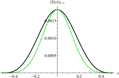
Figure 1: The avalanche shape $\left<S(x)\right>_{\ell=1}$ for $\sigma=1$. The green dotted line is the shape obtained for avalanches with a large aspect ratio $S/\ell^{4}$ at fixed $S$ and $\ell$ in ThieryLeDoussalWiese2015 , rescaled to the same height at $x=0$.

II The probability of a given spatial avalanche shape

Here we review some basic results of Ref. ThieryLeDoussalWiese2015 for the Brownian Force Model. Suppose that the interface is at rest in configuration $u_{1}(x)=u(x,t_{1})$, and then an avalanche occurs which brings it to configuration $u_{2}(x)=u(x,t_{2})$. Denote $S(x):=u_{2}(x)-u_{1}(x)$ the total advance at point $x$, which we call the spatial shape of the avalanche.

We start with a simplified derivation of the key formula of Ref. ThieryLeDoussalWiese2015 , given below in Eq. (14). To this aim, we write the MSR action for the dynamics of the interface, obtained from a time derivative of Eq. (I), as LeDoussalWiese2011a ; LeDoussalWiese2012a ; DobrinevskiLeDoussalWiese2011b

$$\!\!\!\mathrm{e}^{-{\cal S}[\tilde{u},\dot{u}]}=$$ (9)

$$\!\!\!\mathrm{e}^{\int_{x,t}\tilde{u}(x,t)\left[-\partial_{t}\dot{u}(x,t)+\nabla^{2}\dot{u}(x,t)-m^{2}\dot{u}(x,t)+\partial_{t}F(x,u(x,t))+\partial_{t}f(x,t)\right]}.$$

There are no avalanches without driving, and the last term has been added for this purpose. We want to drive the system with a force kick at $t=0$, i.e.

$$f(x,t)=\delta(t)w(x)\ .$$ (10)

Note that compared to the notations in Refs. LeDoussalWiese2011a ; LeDoussalWiese2012a ; DobrinevskiLeDoussalWiese2011b we have absorbed a factor of $m^{2}$ into $w$: Here as in Ref. DelormeLeDoussalWiese2016 it is a kick in the force, there it is a kick in the displacement. Our choice is made so that the limit of $m\to 0$ can be taken later.

To obtain static quantities (as the avalanche-size distribution), one can use a time-independent response field $\tilde{u}(x,t)=\tilde{u}(x)$ LeDoussalWiese2012a ; DobrinevskiLeDoussalWiese2011b . Integrating over times from $t_{1}$ before the avalanche to $t_{2}$ after the avalanche, and using that the interface is at rest at these two moments, yields

$$\mathrm{e}^{-{\cal S}[\tilde{u},u]}=$$ (11)

$$\qquad\mathrm{e}^{\int_{x}\tilde{u}(x)\left[w(x)+\nabla^{2}S(x)-m^{2}S(x)+F(x,u_{2}(x))-F(x,u_{1}(x))\right]}\ .$$

Averaging over disorder, using $\overline{F(x,u)F(x^{\prime},u^{\prime})}=\delta^{d}(x-x^{\prime})\Delta(u-u^{\prime})$, we obtain

$$\!\!\!\overline{\mathrm{e}^{-{\cal S}[\tilde{u},S]}}$$ (12)

$$\qquad=\mathrm{e}^{\int_{x}\tilde{u}(x)\left[w(x)+\nabla^{2}S(x)-m^{2}S(x)\right]+\tilde{u}(x)^{2}[\Delta(0)-\Delta(S(x))]}.$$

Integrating over $\tilde{u}(x)$ yields

$$\int{\cal D}[\tilde{u}]\,\overline{\mathrm{e}^{-{\cal S}[\tilde{u},u]}}\simeq\prod_{x}\frac{1}{\sqrt{\Delta(0)-\Delta(S(x))}}\times$$

$$\qquad\times\exp\!\left({-\frac{\left[\int_{x}w(x)+\nabla^{2}S(x)-m^{2}S(x)\right]^{2}}{4[\Delta(0)-\Delta(S(x))]}}\right).~{}~{}~{}~{}~{}~{}~{}~{}$$ (13)

This formulas is a priori exact for any disorder correlator $\Delta(u)$. For the BFM $\Delta(0)-\Delta(u)\equiv\sigma|u|$. Thus we obtain upon simplification in the limit of $w(x)\to 0$ ThieryLeDoussalWiese2015

$$\mbox{proba}\big{[}S(x)\big{]}\simeq\prod_{x}\frac{1}{\sqrt{S(x)}}\,\mathrm{e}^{-\int_{x}\frac{m^{4}S(x)}{4\sigma}+\frac{[\nabla^{2}S(x)]^{2}}{4\sigma S(x)}}\ .$$ (14)

Changing variables to $\phi(x):=\sqrt{S(x)}$ eliminates the factor of $\prod_{x}S(x)^{-1/2}$. A saddle point for avalanches with a large aspect ratio $S/\ell^{4}$, where $S$ is the avalanches size and $\ell$ its spatial extension, can be obtained by varying w.r.t. $\phi(x)$. The solution of this saddle-point equation is plotted on figure 1 (green dashed line), where it is confronted to the shape for generic avalanches (black) to be derived later. See also figure 12 for a numerical validation of the saddle-point solution in reference ThieryLeDoussalWiese2015 .

III The expectation of $S(x)$ in an avalanche extending from $-\ell/2$ to $\ell/2$

III.1 Generalities

We consider avalanches in the BFM in $d=1$ dimensions. To this aim, we start from Eq. (12), using the correlator (4). This yields

$$\mathrm{e}^{-{\cal S}_{\rm FBM}[\tilde{u},S]}=\mathrm{e}^{\int_{x}\tilde{u}(x)\left[w(x)+\nabla^{2}S(x)-m^{2}S(x)\right]+\sigma\tilde{u}(x)^{2}S(x)}.$$ (15)

We now wish to evaluate the generating function for avalanche sizes

$$\tilde{\cal P}\big{[}\lambda(x)\big{]} := \overline{\mathrm{e}^{\int_{x}\lambda(x)S(x)}}$$ (16)

$$= \int{\cal D}[S]\,{\cal D}[\tilde{u}]\,\mathrm{e}^{\int_{x}\lambda(x)S(x)-{\cal S}_{\rm FBM}[\tilde{u},S]}\ .$$

The crucial remark is that $S(x)$ appears linearly in the exponential; thus integrating over $S(x)$ enforces that $\tilde{u}(x)$ obeys the differential equation DelormeLeDoussalWiese2016

$$\tilde{u}^{\prime\prime}(x)-m^{2}\tilde{u}(x)+\sigma\tilde{u}(x)^{2}=-\lambda(x)\ .$$ (17)

This is an instanton equation. Suppose we have found its solution, which for simplicity we also denote $\tilde{u}(x)$. Then Eq. (16) simplifies considerably to DelormeLeDoussalWiese2016

$$\tilde{\cal P}\big{[}\lambda(x)\big{]}:=\overline{\mathrm{e}^{\int_{x}\lambda(x)S(x)}}=\mathrm{e}^{\int_{x}w(x)\tilde{u}(x)}\ .$$ (18)

In Ref. DelormeLeDoussalWiese2016 , a solution for $\lambda(x)$ in the form

$$\lambda(x)=-\lambda_{1}\delta(x-r_{1})-\lambda_{2}\delta(x-r_{2})$$ (19)

was given in the limit of $\lambda_{1,2}\to\infty$. This solution ensures that if the interface has moved at positions $r_{1}$ or $r_{2}$, the expression ${\mathrm{e}^{\int_{x}\lambda(x)S(x)}}$ is 0; otherwise it is 1. The probability that the interface has not moved at these two positions $r_{1}$ and $r_{2}$ thus is

$$\tilde{\cal P}_{r_{1},r_{2}}=\mathrm{e}^{\int_{x}w(x)\tilde{u}(x)}\ .$$ (20)

We now consider driving at $x$ between the two points $r_{1}$ and $r_{2}$. In order that the probability (20) decreases for an increase in the driving at $x$, we need that

$$\tilde{u}(x)<0\ ,\qquad r_{1}<x<r_{2}\ .$$ (21)

This helps us to select the correct solution, see appendix A. Call $\tilde{u}_{0}(x)$ this solution. According to DelormeLeDoussalWiese2016 , it reads

$$\tilde{u}_{0}(x)=\frac{1}{(r_{2}-r_{1})^{2}}\,f\!\left(\frac{2x-r_{1}-r_{2}}{2(r_{2}-r_{1})}\right)\ .$$ (22)

Its extension is

$$\ell=r_{2}-r_{1}\ .$$ (23)

It further depends on the dimensionless combination $\frac{\ell}{L_{m}}=\ell m$. In the massless limit, i.e. for

$$\frac{\ell}{L_{m}}=\ell m\ll 1\ ,$$ (24)

the function $f(x)$ satisfies Eq. (17) for $m=0$, i.e.

$$f^{\prime\prime}(x)+f(x)^{2}=0\ .$$ (25)

This solution diverges with a quadratic divergence at $x=\pm 1/2$. We review in appendix A its construction. We see there that it is a negative-energy solution with energy $-\bar{\cal E}_{1}$, where

$$\bar{\cal E}_{1}=\frac{8\pi^{3}\Gamma\left(\frac{1}{3}\right)^{6}}{3\Gamma\left(\frac{5}{6}\right)^{6}}\ .$$ (26)

It reads

$$\ f(x)=-6\,{\cal P}\!\left(x+1/2;g_{2}=0,g_{3}=\frac{\Gamma\left(\frac{1}{3}\right)^{18}}{(2\pi)^{6}}\right)\ .$$ (27)

The function ${\cal P}$ is the Weierstrass $\cal P$ function. The parameter $g_{3}$ satisfies

$$g_{3}\equiv\frac{\bar{\cal E}_{1}}{18}\ ,$$ (28)

and the solution respects the constraint (21). For later simplifications we note the following relations

$$\frac{2}{3}f^{3}(x)+f^{\prime}(x)^{2}=-36g_{3}\equiv-2{\bar{\cal E}_{1}}\ .$$ (29)

$$\frac{2}{3}f(x)f^{\prime\prime}(x)-f^{\prime}(x)^{2}=36g_{3}=2\bar{\cal E}_{1}\ .$$ (30)

III.2 Driving

Let us now specify the driving function $w(x)$ introduced in Eq. (10). There are two main choices:

• uniformly distributed random seeds (random localized driving)

  $$w(x)=w\,\delta(x-x_{\rm s})\ .$$ (31)

  Here we first calculate the observable at hand, and finally average, i.e. integrate, over the seed position $x_{\rm s}$. In a numerical experiment, one can take a random permutation of the $N$ degrees of freedom, and then apply a kick to each of them in the chosen order.

• uniform driving

  $$w(x)=w\ .$$ (32)

As we wish to work at first non-vanishing order in $w$, this makes almost no difference. Indeed, in Eq. (18) we formally have for both driving protocols to leading order in $w$

$$\overline{\mathrm{e}^{\int_{x}\lambda(x)S(x)}-1}=\mathrm{e}^{\int_{x}w(x)\tilde{u}(x)}-1\to w\int_{x}\tilde{u}(x)\ .$$ (33)

There is however one caveat: If $\tilde{u}(x)\to-\infty$, as is the case for solution (22) at $x=r_{1,2}$, then, for localized driving, points $x$ around these singularities are suppressed, and the corresponding points have to be taken out of the integral. On the other hand, for uniform driving, the middle integral in Eq. (33) simply vanishes. In that case one has to regularize the solution, i.e. work at finite $\lambda_{1,2}$, then take $w\to 0$, and only at the end take the limit $\lambda_{1,2}\to\infty$. According to appendix A, working at finite $\lambda_{1,2}$ is equivalent to cutting out a piece of size $x_{0}$ around the singularity, with $x_{0}$ given by Eq. (100). Thus, effectively, driving is restricted to the interval $[r_{1}+x_{0},r_{2}-x_{0}]$ slightly smaller than the the full interval $[r_{1},r_{2}]$.

For conceptual clarity, and simplicity of presentation, we will work with uniformly distributed random seeds (random localized driving) below. The idea to keep in mind is that in the limit $w\to 0$, the driving only triggers the avalanche, but after the avalanche starts, its subsequent dynamics is independent of the driving. As a result, the avalanche shape is independent of the driving and we can choose the most convenient driving.

III.3 Strategy of the calculation

We now want to construct perturbatively a solution of Eq. (17) at $m=0$, and $\sigma=1$. i.e.

$$\tilde{u}^{\prime\prime}(x)+\tilde{u}(x)^{2}=-\lambda(x)\ ,$$ (34)

with

$$\lambda(x)=-\lambda_{1}\delta(x-r_{1})-\lambda_{2}\delta(x-r_{2})+\eta\delta(x-x_{\rm c})\ ,$$ (35)

$$\lambda_{1},\lambda_{2}\to\infty\ .$$ (36)

We are interested in the limit of vanishing $\eta$, i.e. at first and second order in $\eta$. This instanton solution will have the form

$$\tilde{u}(x)=\tilde{u}_{0}(x)+\eta\tilde{u}_{1}(x)+\eta^{2}\tilde{u}_{2}(x)+...\ .$$ (37)

It will be continuous, but non-analytic at $x=x_{\rm c}$, see Fig 2.

Let us reconsider Eq. (18), i.e. $\overline{\mathrm{e}^{\int_{x}\lambda(x)S(x)}}=\mathrm{e}^{\int_{x}w(x)\tilde{u}(x)}$. Its l.h.s. can be written as

$$\overline{\mathrm{e}^{\int_{x}\lambda(x)S(x)}} = \int_{r_{1}}^{x_{\rm c}}\mathrm{d}r_{\rm left}\int^{r_{2}}_{x_{\rm c}}\mathrm{d}r_{\rm right}\int_{0}^{\infty}{\mathrm{d}}S(x_{c})\,$$ (38)

$$\qquad\mathrm{e}^{\eta S(x_{c})}{\cal P}(S(x_{c}),r_{\rm left},r_{\rm right})\ ,\qquad\qquad$$

where ${\cal P}(S(x_{c}),r_{\rm left},r_{\rm right})$ is the joint probability that the avalanche has advanced by $S(x_{\rm c})$ at $x_{c}$, and that it extends from $r_{\rm left}$ to $r_{\rm right}$, with $r_{1}<r_{\rm left}<x_{\rm c}<r_{\rm right}<r_{2}$.

Taking derivatives w.r.t. points $r_{1}$ and $r_{2}$ yields

$$\!\!\!-\frac{\partial^{2}}{\partial{r_{1}}\partial r_{2}}\,\overline{\mathrm{e}^{\int_{x}\lambda(x)S(x)}}$$

$$\quad=\int_{0}^{\infty}{\mathrm{d}}S(x_{c})\,\mathrm{e}^{\eta S(x_{c})}{\cal P}(S(x_{c}),r_{\rm left},r_{\rm right})$$

$$\quad=P_{\ell}(r_{2}-r_{1})\left<\mathrm{e}^{\eta S(x_{c})}\right>_{\!r_{1}}^{\!r_{2}}$$

$$\quad=P_{\ell}(r_{2}-r_{1})\left[1+\eta\langle S(x_{c})\rangle_{r_{1}}^{r_{2}}+\frac{\eta^{2}}{2}\langle S(x_{c})^{2}\rangle_{r_{1}}^{r_{2}}+...\right].$$

Here $P_{\ell}(\ell)$ is the probability to have an avalanche with extension $\ell$, and angular brackets $\langle...\rangle_{r_{1}}^{r_{2}}$ denote conditional averages given that the endpoints of the avalanches are at $r_{1}$ and $r_{2}$.

We now consider derivatives w.r.t. points $r_{1}$ and $r_{2}$ of the r.h.s. of Eq. (18). Using the expansion (37) yields

$$\!\!\!-\frac{\partial^{2}}{\partial{r_{1}}\partial r_{2}}\mathrm{e}^{\int_{x}w(x)\tilde{u}(x)}=-\mathrm{e}^{\int\mathrm{d}x\,w(x)\tilde{u}_{0}(x)}$$

$$\qquad\times\Big{[}\int\mathrm{d}x\,w(x)\frac{\partial^{2}\tilde{u}_{0}(x)}{\partial r_{1}\partial r_{2}}+\eta\int\mathrm{d}x\,w(x)\frac{\partial^{2}\tilde{u}_{1}(x)}{\partial r_{1}\partial r_{2}}$$

$$\qquad~{}~{}+\eta^{2}\int\mathrm{d}x\,w(x)\frac{\partial^{2}\tilde{u}_{2}(x)}{\partial r_{1}\partial r_{2}}+...\Big{]}$$ (40)

Omitted terms indicated by $...$ are higher order in $w$. Comparing Eqs. (III.3) and (III.3) yields for the probability to find an avalanche with extension $\ell$

$$P_{\ell}(\ell=r_{2}-r_{1})=-\mathrm{e}^{\int\mathrm{d}x\,w(x)\tilde{u}_{0}(x)}\int\mathrm{d}x\,w(x)\frac{\partial^{2}\tilde{u}_{0}(x)}{\partial r_{1}\partial r_{2}}+...$$ (41)

We now have to specify the driving. Following the discussion in section III.2, we either have to use uniform driving restricted to $[r_{1}+x_{0},r_{2}-x_{0}]$, or choose random seeds $x_{\rm s}$ uniformly distributed between $r_{1}$ and $r_{2}$. Here we write formulas for the latter, choosing $w(x)=w\delta(x-x_{s})$. This yields

$$P_{\ell}(\ell=r_{2}-r_{1})=-w\int_{r_{1}}^{r_{2}}\mathrm{d}x_{\rm s}\,\mathrm{e}^{w\tilde{u}_{0}(x_{\rm s})}\frac{\partial^{2}\tilde{u}_{0}(x_{\rm s})}{\partial r_{1}\partial r_{2}}+...$$ (42)

In the limit of small $w$ this becomes

$$P_{\ell}(\ell=r_{2}-r_{1})=-w\int_{r_{1}}^{r_{2}}\mathrm{d}x_{\rm s}\,\frac{\partial^{2}\tilde{u}_{0}(x_{\rm s})}{\partial r_{1}\partial r_{2}}+...$$ (43)

Dropping the index s for the seed position, the final formulas for the observables of interest are

$$\!\!P_{\ell}(\ell=r_{2}-r_{1})=-w\int_{r_{1}}^{r_{2}}\mathrm{d}x\,\frac{\partial^{2}\tilde{u}_{0}(x)}{\partial r_{1}\partial r_{2}}$$ (44)

$$\!\!P_{\ell}(\ell=r_{2}-r_{1})\left<S(x_{c})\right>_{\!r_{1}}^{\!r_{2}}=-w\int_{r_{1}}^{r_{2}}\mathrm{d}x\,\frac{\partial^{2}\tilde{u}_{1}(x)}{\partial r_{1}\partial r_{2}}$$ (45)

$$\!\!P_{\ell}(\ell=r_{2}-r_{1})\frac{1}{2}\left<S(x_{c})^{2}\right>_{\!r_{1}}^{\!r_{2}}=-w\int_{r_{1}}^{r_{2}}\mathrm{d}x\,\frac{\partial^{2}\tilde{u}_{2}(x)}{\partial r_{1}\partial r_{2}}$$ (46)

The shape and its variance are thus given by the ratios of the above equation.

The following calculations are structured as follows: In the next subsection, we give the instanton solution (34) for extension $\ell=1$; more precisely $r_{1}=-1/2$, $r_{2}=1/2$.

In a second step performed in section IV, we reconstruct the solution for general $r_{1}$ and $r_{2}$. This allows us to vary as in Eq. (III.3) w.t.t. $r_{1}$ and $r_{2}$, thus selecting only those avalanches which touch the borders at $r_{1}$ and $r_{2}$. With the normalization (25) obtained from the probability to find an avalanche of extension $\ell$ performed in subsection IV.1, this allows us to give the normalized shape, and its fluctuations in subsection IV.3.

III.4 How to obtain the mean shape of all avalanches inside a box of size 1, and its fluctuations

We now solve Eq. (34) at $r_{1}=-1/2$, $r_{2}=1/2$.

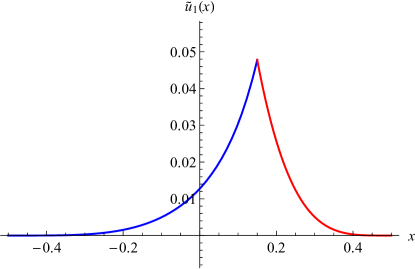
Figure 2: The solutions (37) at order $\eta$ for $x_{\rm c}=0.15$. Note that $\tilde{u}_{1}(x)$ grows with a quartic power close to the boundary.

One can write down differential equations to be solved by $\tilde{u}_{1}(x)$ and $\tilde{u}_{2}(x)$. There is, however, a more elegant way to derive the perturbed instanton solution: To achieve this, we first realize that if $\tilde{u}(x)$ is a solution of $\tilde{u}^{\prime\prime}(x)+\tilde{u}(x)^{2}=0$, then $\tilde{u}_{\lambda,c}(x):=\lambda^{2}\tilde{u}(\lambda x+c)$ is also a solution. We wish to construct solutions which diverge at $x=\pm 1/2$, i.e. have extension 1, and which produce the additional term proportional to $\eta$ in Eq. (35). This can be achieved by separate solutions for the left branch, i.e. $-1/2<x<x_{\rm c}$, and the right branch $x_{\rm c}<x<1/2$. Using the symbol $f$ to indicate extension 1 as in Eq. (27), we have

$$f_{\lambda_{\rm L}}^{\rm L}(x) := \lambda_{\rm L}^{2}f\big{(}\lambda_{\rm L}(x+1/2)-1/2\big{)}$$ (47)

$$x_{\lambda_{\rm L}}^{\rm L}(f) = \lambda_{\rm L}^{-1}x(\lambda_{\rm L}^{-2}f)+\frac{1}{2}\left(\frac{1}{\lambda_{\rm L}}-1\right)$$ (48)

$$f_{\lambda_{\rm R}}^{\rm R}(x) := \lambda_{\rm R}^{2}f\big{(}{\lambda_{\rm R}}(x-1/2)+1/2\big{)}$$ (49)

$$x_{\lambda_{\rm R}}^{\rm R}(f) = \lambda_{\rm R}^{-1}x(\lambda_{\rm R}^{-2}f)-\frac{1}{2}\left(\frac{1}{\lambda_{\rm R}}-1\right)\ .~{}~{}$$ (50)

The two functions must coincide at $x_{\rm c}$, and their slope must change by $\eta$; more precisely

$$f_{\lambda_{\rm L}}^{\rm L}(x_{\rm c})=f_{\lambda_{\rm R}}^{\rm R}(x_{\rm c})\ ,$$ (51)

$$\partial_{x}f_{\lambda_{\rm L}}^{\rm L}(x)\Big{|}_{x=x_{\rm c}}=\partial_{x}f_{\lambda_{\rm R}}^{\rm R}(x)\Big{|}_{x=x_{\rm c}}+\eta\ .$$ (52)

The second equation is written in a way to make clear that while $\lambda_{\rm L}$ and $\lambda_{\rm R}$ depend on $x_{\rm c}$, this dependence is not included in the derivatives of Eq. (52). We make the ansatz

$$\lambda_{\rm L} = 1+a\eta+c\eta^{2}\ ,$$ (53)

$$\lambda_{\rm R} = 1+b\eta+d\eta^{2}\ .$$ (54)

Repeatedly using Eqs. (25), (29) and (30) to eliminate higher derivatives, we find

$$a = \frac{(2x_{\rm c}-1)f^{\prime}(x_{\rm c})+4f(x_{\rm c})}{12\bar{\mathcal{E}}_{1}}$$ (55)

$$b = \frac{(2x_{\rm c}+1)f^{\prime}(x_{\rm c})+4f(x_{\rm c})}{12\bar{\mathcal{E}}_{1}}$$ (56)

$$c = \frac{1}{288\bar{\mathcal{E}}_{1}^{2}}\Big{[}16f(x_{\rm c})\left((1-3x_{\rm c})f^{\prime}(x_{\rm c})\right)$$ (57)

$$+(2x_{\rm c}-1)\Big{(}f^{\prime}(x_{\rm c})\Big{(}\left(4x_{\rm c}^{2}-1\right)f^{\prime\prime}(x_{\rm c})$$

$$+4\left(3x_{\rm c}+1\right)f^{\prime}(x_{\rm c})\Big{)}+24\bar{\mathcal{E}}_{1}x_{\rm c}\Big{)}-96f(x_{\rm c})^{2}\Big{]}~{}~{}~{}~{}~{}$$

$$d = \frac{1}{288\bar{\mathcal{E}}_{1}^{2}}\Big{[}16f(x_{\rm c})(-(3x_{\rm c}+1)f^{\prime}(x_{\rm c}))-96f(x_{\rm c})^{2}$$ (58)

$$+(2x_{\rm c}+1)\Big{(}f^{\prime}(x_{\rm c})\Big{(}\left(4x_{\rm c}^{2}-1\right)f^{\prime\prime}(x_{\rm c})$$

$$+4\left(3x_{\rm c}-1\right)f^{\prime}(x_{\rm c})\Big{)}+24\bar{\mathcal{E}}_{1}x_{\rm c}\Big{)}\Big{]}~{}~{}~{}~{}~{}\ .$$

This gives

$$f_{\lambda_{\rm L}}^{\rm L}(x) = f(x)+\eta\frac{a}{2}\Big{[}(2x+1)f^{\prime}(x)+4f(x)\Big{]}+\frac{\eta^{2}}{8}\Big{[}8(a^{2}+2c)f(x)+4(2x+1)(2a^{2}+c)f^{\prime}(x)+a^{2}(2x+1)^{2}f^{\prime\prime}(x)\Big{]}$$ (59)

$$+O(\eta^{3})$$

$$f_{\lambda_{\rm R}}^{\rm R}(x) = f(x)+\eta\frac{b}{2}\Big{[}(2x-1)f^{\prime}(x)+4f(x)\Big{]}+\frac{\eta^{2}}{8}\Big{[}8(b^{2}+2d)f(x)+4(2x-1)(2b^{2}+d)f^{\prime}(x)+b^{2}(2x-1)^{2}f^{\prime\prime}(x)\Big{]}$$ (60)

$$+O(\eta^{3})\ .$$

For illustration we plot on Fig. 2 the order-$\eta$ solution for $x_{\rm c}=0.15$.

We are finally interested in uniformly distributed random seeds, i.e. we need to integrate these solutions over the driving point $x$ inside the box, i.e. from $-1/2$ to $1/2$. To this purpose define

$$F(x):=6\zeta\!\left(\!x+\frac{1}{2};0,\frac{\Gamma\left(\frac{1}{3}\right)^{18}}{64\pi^{6}}\right)-F_{0}\ ,\qquad F_{0}=6\zeta\!\left(\!\frac{1}{2};0,\frac{\Gamma\left(\frac{1}{3}\right)^{18}}{64\pi^{6}}\right)\equiv 2\pi\sqrt{3}\ ,\qquad F^{\prime}(x)=f(x)$$ (61)

$$F(0)=0\ ,\qquad F(x+1)=F(x)+2F_{0}\ .$$ (62)

Then, subtracting the solution at $\eta=0$ which is not needed (but whose integral is divergent), we obtain

$$\int_{-\frac{1}{2}}^{x_{\rm c}}\mathrm{d}x\,\left[f_{\lambda_{\rm L}}^{\rm L}(x)-f(x)\right] = \eta a\Big{[}\frac{1}{2}(2x_{\rm c}+1)f(x_{\rm c})+F_{0}+F(x_{\rm c})\Big{]}$$

$$+\eta^{2}\Big{[}\frac{1}{8}a^{2}(2x_{\rm c}+1)^{2}f^{\prime}(x_{\rm c})+\frac{1}{2}(a^{2}+c)(2x_{\rm c}+1)f(x_{\rm c})+c\big{(}F(x_{\rm c})+F_{0}\big{)}\Big{]}$$

$$\int_{x_{\rm c}}^{\frac{1}{2}}\mathrm{d}x\,\left[f_{\lambda_{\rm R}}^{\rm R}(x)-f(x)\right] = \eta b\Big{[}\frac{1}{2}(1-2x_{\rm c})f(x_{\rm c})+F_{0}-F(x_{\rm c})\Big{]}$$ (63)

$$+\eta^{2}\Big{[}-\frac{1}{2}(b^{2}+d)(2x_{\rm c}-1)f(x_{\rm c})-\frac{1}{8}b^{2}(2x_{\rm c}-1)^{2}f^{\prime}(x_{\rm c})+d\big{(}F_{0}-F(x_{\rm c})\big{)}\Big{]}\ .$$

This yields the (unnormalized) expectation, given that the interface has not moved at points $\pm 1/2$:

$$\left<\mathrm{e}^{\eta S(x_{\rm c})}-1\right>=w\int_{-\frac{1}{2}}^{x_{\rm c}}\mathrm{d}x\,\left[f_{\lambda_{\rm L}}^{\rm L}(x)-f(x)\right]+w\int_{x_{\rm c}}^{\frac{1}{2}}\mathrm{d}x\,\left[f_{\lambda_{\rm R}}^{\rm R}(x)-f(x)\right]$$

$$=w\eta\Big{[}\frac{1}{2}f\left(x_{\rm c}\right)\Big{(}2(a-b)x_{\rm c}+a+b\Big{)}+(a-b)F(x_{\rm c})+(a+b)F_{0}\Big{]}$$

$$~{}~{}~{}~{}+w\frac{\eta^{2}}{8}\bigg{[}4f(x_{\rm c})\Big{(}2x_{\rm c}(a^{2}-b^{2}+c-d)+a^{2}+b^{2}+c+d\Big{)}+\Big{(}2(a-b)x_{\rm c}+a+b\Big{)}\Big{(}2(a+b)x_{\rm c}+a-b\Big{)}f^{\prime}(x_{\rm c})$$

$$~{}~{}~{}~{}\qquad~{}~{}~{}+8(c-d)F(x_{\rm c})+8(c+d)F_{0}\big{)}\bigg{]}+...$$

$$=w\eta\,\frac{2f(x_{\rm c})\big{[}f(x_{\rm c})+2F_{0}\big{]}-\big{[}F(x_{\rm c})-2F_{0}x_{\rm c}\big{]}f^{\prime}(x_{\rm c})}{6\bar{\mathcal{E}}_{1}}$$

$$~{}~{}~{}~{}+w\frac{\eta^{2}}{144\bar{\mathcal{E}}_{1}^{2}}\bigg{[}-4x_{\rm c}F(x_{\rm c})\Big{(}6\bar{\mathcal{E}}_{1}+f^{\prime}(x_{\rm c})^{2}\Big{)}+4F_{0}\Big{(}12\bar{\mathcal{E}}_{1}x_{\rm c}^{2}+(6x_{\rm c}^{2}-1)f^{\prime}(x_{\rm c})^{2}\Big{)}+f(x_{\rm c})^{2}\Big{(}8x_{\rm c}f^{\prime}(x_{\rm c})-96F_{0}\Big{)}$$

$$~{}~{}~{}~{}+f(x_{\rm c})f^{\prime}(x_{\rm c})\Big{(}3(4x_{\rm c}^{2}-1)f^{\prime}(x_{\rm c})+16F(x_{\rm c})-48F_{0}x_{\rm c}\Big{)}+(4x_{\rm c}^{2}-1)\Big{(}2F_{0}x_{\rm c}-F(x_{\rm c})\Big{)}f^{\prime}(x_{\rm c})f^{\prime\prime}(x_{\rm c})-32f(x_{\rm c})^{3}\bigg{]}$$

$$~{}~{}~{}~{}+...$$

$$=:w\eta S_{\rm box}^{\ell=1}(x_{\rm c})+w\frac{\eta^{2}}{2}S_{\rm box}^{2,\ell=1}(x_{\rm c})+...\ .$$ (64)

We have termed these expressions $S_{\rm box}^{\ell=1}(x_{\rm c})$ and $S_{\rm box}^{2,\ell=1}(x_{\rm c})$. We recall that this is not yet the sought-for avalanche shape, and fluctuations. Rather, it is the expectation of the size $S(x)$ inside a box of size $1$, given that the avalanche does not touch any of the two boundaries $x=\pm 1/2$. We will have to vary the boundary points in order to extract the shape $\left<S(x)\right>$ of avalanches which vanish at the boundary points, but not before. This is the objective of the next section.

For later reference, we note

$$\int_{-\frac{1}{2}}^{\frac{1}{2}}\mathrm{d}x\,S_{\rm box}(x)=$$

$$=-\frac{3f^{\prime}(x)+f(x)F(x)-2F_{0}(xf(x)+F(x))}{6\bar{\mathcal{E}}_{1}}\Bigg{|}_{-\frac{1}{2}}^{\frac{1}{2}}$$

$$=\frac{2F_{0}^{2}}{3\bar{\mathcal{E}}_{1}}=\frac{256\pi^{8}}{9\Gamma(\frac{1}{3})^{18}}=0.00534401\ ,$$ (65)

$$\int_{-\frac{1}{2}}^{\frac{1}{2}}\mathrm{d}x_{\rm c}\,S_{\rm box}^{2,\ell=1}(x_{\rm c})=2.3030\times 10^{-6}\ .$$ (66)

IV From $S_{\rm box}(x)$ to the shape $S(x)$: Scaling arguments, etc.

IV.1 The probability to find an avalanche of extension $\ell$, and probability for seed position

The probability to have an avalanche of size $\ell$ is according to Eqs. (22) and (25) to leading order in $w$ given by

$$P_{\ell}(\ell)=-w\int_{r_{1}}^{r_{2}}\mathrm{d}x\,\frac{\partial^{2}\tilde{u}_{0}(x)}{\partial r_{1}\partial r_{2}}$$

$$=\frac{w}{\ell^{3}}\int_{-\frac{1}{2}}^{\frac{1}{2}}\mathrm{d}x\,\frac{(4x^{2}-1)f^{\prime\prime}(x)+24(xf^{\prime}(x)+f(x))}{4}+...$$

$$\simeq 4F_{0}\frac{w}{\ell^{3}}+...\equiv 8\pi\sqrt{3}\frac{w}{\ell^{3}}+...\ ,$$ (67)

with $F_{0}$ defined in Eq. (61).

It is interesting to note that the integrand in Eq. (67) gives the probability to have the seed at position $x$. More precisely, the probability that the seed was at position $x$ inside an avalanche extending from $-1/2$ to $1/2$ is

$$P^{\rm seed}_{\ell=1}(x)=\frac{(4x^{2}-1)f^{\prime\prime}(x)+24[xf^{\prime}(x)+f(x)]}{32\pi\sqrt{3}}\ .$$ (68)

This function starts with a cubic power at the boundary. We give a series expansion below in Eq. (88).

IV.2 Basic scaling relations, and consequences

In general, the size of an avalanche scales as $S(\ell)\sim\ell^{{d+\zeta}}$. For the BFM, the latter reduces to

$$S(\ell)\sim\ell^{4}\ .$$ (69)

The proportionality constant is calculated in Eq. (80) below.

Let us now solve the instanton equation (34) with source (35) for arbitrary $r_{1}$ and $r_{2}$. This can be achieved by observing that, as a function of $|r_{2}-r_{1}|$,

$$\tilde{u}^{\prime\prime}(x) \sim \tilde{u}(x)^{2}\sim\frac{1}{|r_{2}-r_{1}|^{4}}$$ (70)

$$\sim \eta\delta(x-x_{c})\equiv\frac{\eta}{|r_{2}-r_{1}|}\delta\left(\frac{x-x_{c}}{|r_{2}-r_{1}|}\right)\ .~{}~{}~{}$$

Thus $\eta\sim|r_{2}-r_{1}|^{-3}$, and

$$\tilde{u}^{x_{\rm c}}_{1,r_{2},r_{1}}(x)=|r_{2}-r_{1}|\,\tilde{u}^{\frac{x_{\rm c}-(r_{1}+r_{2})/2}{r_{2}-r_{1}}}_{1,r_{1/2}=\mp\frac{1}{2}}\Big{(}\textstyle{\frac{x-(r_{1}+r_{2})/2}{r_{2}-r_{1}}}\Big{)}\ ,$$ (71)

$$\!\!\Rightarrow S_{\rm box}^{r_{1},r_{2}}(x_{\rm c})=\int_{r_{1}}^{r_{2}}\mathrm{d}x\,\tilde{u}^{x_{\rm c}}_{1,r_{2},r_{1}}(x)$$

$$\hphantom{\Rightarrow S_{\rm box}^{r_{1},r_{2}}(x_{\rm c})}=|r_{2}-r_{1}|^{2}\,S_{\rm box}^{r_{2}-r_{1}=1}\Big{(}\textstyle{\frac{x_{\rm c}-(r_{1}+r_{2})/2}{r_{2}-r_{1}}}\Big{)}\ .$$ (72)

This is consistent with the dimension of an avalanche $S$ per length $\ell$, i.e. $S/\ell\sim\ell^{3}$.

Now, the (unnormalized) shape of an avalanche of extension $\ell$ is according to Eq. (45) obtained as

$$S_{\ell=r_{2}-r_{1}}(x) = -\partial_{r_{2}}\partial_{r_{1}}S^{r_{2},r_{1}}_{\rm box}(x)\ .$$ (73)

Using Eq. (71), this yields

$$S_{\ell=1}(x) = -\partial_{r_{2}}\partial_{r_{1}}\Big{[}|r_{2}{-}r_{1}|^{2}S_{\rm box}^{\ell=1}\Big{(}\textstyle{\frac{x-(r_{1}+r_{2})/2}{r_{2}-r_{1}}}\Big{)}\Big{]}_{r_{1}=-\frac{1}{2}}^{r_{2}=\frac{1}{2}}$$ (74)

$$= \Big{[}2-2x\,\partial_{x}+\Big{(}x^{2}-\frac{1}{4}\Big{)}\partial_{x}^{2}\Big{]}S_{\rm box}^{\ell=1}(x)\ .$$

We note that this function grows cubicly at the boundary, consistent with our scaling argument (6). To achieve this, the factor of $|r_{2}{-}r_{1}|^{2}$ in Eq. (74) is crucial: Were the exponent larger than $2$, then the growth would be linear. Were it smaller, the function (74) would become negative.

Integrating by parts we obtain using Eq. (III.4)

$$\int_{-\frac{1}{2}}^{\frac{1}{2}}\mathrm{d}x\,S_{\ell=1}(x)=6\int_{-\frac{1}{2}}^{\frac{1}{2}}\mathrm{d}x_{\rm c}\,S_{{\rm box}}^{\ell=1}(x_{\rm c})=\frac{4F_{0}^{2}}{\bar{\mathcal{E}}_{1}}\ .$$ (75)

Similarly, we find for the order-$\eta^{2}$ term

$$S^{2}_{\ell=1}(x) = -\partial_{r_{2}}\partial_{r_{1}}\Big{[}|r_{2}{-}r_{1}|^{5}S_{\rm box}^{2,\ell=1}\Big{(}\textstyle{\frac{x-(r_{1}+r_{2})/2}{r_{2}-r_{1}}}\Big{)}\Big{]}_{r_{1}=-\frac{1}{2}}^{r_{2}=\frac{1}{2}}$$ (76)

$$= \Big{[}20-8x\,\partial_{x}+\Big{(}x^{2}-\frac{1}{4}\Big{)}\partial_{x}^{2}\Big{]}S_{\rm box}^{2,\ell=1}(x)\ .$$

This implies

$$\int_{-\frac{1}{2}}^{\frac{1}{2}}\mathrm{d}x\,S^{2,\ell=1}(x)=30\int_{-\frac{1}{2}}^{\frac{1}{2}}\mathrm{d}x_{\rm c}\,S_{{\rm box}}^{2,\ell=1}(x_{\rm c})\ .$$ (77)

Note that according to Eqs. (44)-(46) $S_{\ell}(x)$ and $S_{\ell}^{2}(x)$ are not yet properly normalized to give the expectation of the shape of an avalanche. For this purpose, let us define with the help of Eq. (67)

$$\left<{S(x)}\right>_{\ell} := \frac{w{S_{\ell}(x)}}{P_{\rm aval}(\ell)}=\frac{S_{\ell=1}(x/\ell)}{4F_{0}}\ell^{3}\ ,$$ (78)

$$\left<{S^{2}(x)}\right>_{\ell} := \frac{w{S_{\ell}^{2}(x)}}{P_{\rm aval}(\ell)}=\frac{S^{2}_{\ell=1}(x/\ell)}{4F_{0}}\ell^{6}\ .$$ (79)

These functions give the shape of an avalanche given that the avalanche extends from $-\frac{1}{2}$ to $\frac{1}{2}$, as well as its fluctuations, including the amplitude.

For the total size $\left<S\right>_{\ell}=\int_{-\frac{\ell}{2}}^{\frac{\ell}{2}}\mathrm{d}x\,\left<S(x)\right>_{\ell}$ and the integral of the second moment $\left<S^{2}(x)\right>_{\ell}$ we find

$${\int_{-\frac{\ell}{2}}^{\frac{\ell}{2}}\mathrm{d}x\left<{S(x)}\right>_{\ell}}=\frac{F_{0}}{\bar{\cal E}_{1}}\ell^{4}=0.000736576\,\ell^{4}\ ,$$ (80)

$${\int_{-\frac{\ell}{2}}^{\frac{\ell}{2}}\mathrm{d}x\left<{S^{2}(x)}\right>_{\ell}}=5.29044\times 10^{-8}\,\ell^{7}\ .$$ (81)

IV.3 Results for the shape and its second moment

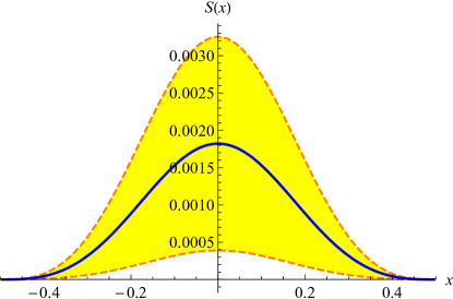
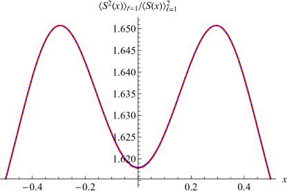
Figure 3: Left: The spatial shape $\left<S(x)\right>_{\ell=1}$ of an avalanche conditioned conditioned to have size $\ell=1$ (blue, solid line). The dashed curves represent $\left<S(x)\right>_{\ell=1}\pm\sqrt{\left<{S_{\ell}^{2}(x)}\right>_{\ell=1}^{\rm c}}$. Right: The ratio $\left<{S_{\ell}^{2}(x)}\right>_{\ell=1}/\left<{S_{\ell}(x)}\right>_{\ell=1}^{2}$, which has spatial average (integeral) $1.63523384$; blue from an interpolating function, red dashed from series expansion with the 16 leading terms; note that below in Eq. (87) only the leading 8 are given.

We give explicit formulas for $\left<S(x)\right>_{\ell=1}$, and $\left<S^{2}(x)\right>_{\ell=1}$ below. They are plotted on Fig. 3. We did not succeed in finding much simpler expressions. While especially the expression for the second moment $\left<S^{2}(x)\right>_{\ell=1}$ is lengthy, its ratio with the squared first moment is almost constant, given by

$$\frac{\left<S^{2}(x)\right>_{\ell=1}}{\left<S(x)\right>_{\ell=1}^{2}}\approx 1.635\pm 0.02\ .$$ (82)

This can be seen on Fig. 3. The explicit formulas are

$$\left<{S(x)}\right>_{\ell=1}=\frac{1}{48F_{0}\bar{\mathcal{E}}_{1}}\bigg{[}3(4x^{2}-1)\bar{\mathcal{E}}_{1}-\Big{(}f(x)(-4x^{2}F(x)+F(x)+12x)+2F_{0}x((4x^{2}-1)f(x)+8)+4F(x)\Big{)}f^{\prime}(x)$$

$$\qquad\qquad\qquad\qquad\quad+3(4x^{2}-1)f^{\prime}(x)^{2}+4f(x)(f(x)(-x(F(x)+2F_{0}x)+F_{0}+2)+4F_{0})\bigg{]}\ ,$$ (83)

$$\left<{S^{2}(x)}\right>_{\ell=1}=\frac{1}{576F_{0}\bar{\mathcal{E}}_{1}^{2}}\bigg{[}F(x)(-1344x\bar{\mathcal{E}}_{1}+(1-4x^{2})^{2}f^{\prime}(x)^{3}-736xf^{\prime}(x)^{2})$$

$$+2F_{0}\Big{(}192(3x^{2}\bar{\mathcal{E}}_{1}+\bar{\mathcal{E}}_{1})+(-(1-4x^{2})^{2}xf^{\prime}(x)+384x^{2}+88)f^{\prime}(x)^{2}\Big{)}$$

$$+f(x)\Big{(}24(12x^{2}+1)\bar{\mathcal{E}}_{1}-4((8x^{3}-2x)F(x)+F_{0}(32x^{4}-20x^{2}+3)+72x^{2}+18)f^{\prime}(x)^{2}+640(F(x)+3F_{0}x)f^{\prime}(x)\Big{)}$$

$$-6x(4x^{2}-1)f^{\prime}(x)\Big{(}14\bar{\mathcal{E}}_{1}+9f^{\prime}(x)^{2}\Big{)}+4f(x)^{3}\Big{(}(4x^{2}-1)(-4x^{2}F(x)+2F_{0}(4x^{2}-1)x+F(x)-2x)f^{\prime}(x)-320\Big{)}$$

$$+f(x)^{2}\Big{(}f^{\prime}(x)(-11(1-4x^{2})^{2}f^{\prime}(x)-4(52x^{2}+3)F(x)+1472x)+16F_{0}(x(52x^{2}-5)f^{\prime}(x)-240)\Big{)}$$

$$+f(x)^{4}\Big{(}4x(4x^{2}-1)F(x)+F_{0}(64x^{4}-40x^{2}+6)+8(28x^{2}-3)\Big{)}+2(1-4x^{2})^{2}f(x)^{5}\bigg{]}\ .$$ (84)

While these expressions are cumbersome, one can work with a converging Taylor series. An expansion in $(\frac{1}{2}-x)(\frac{1}{2}+x)$ respecting the Taylor expansion at the boundary is

$$\left<{S(x)}\right>_{\ell=1} = \frac{1}{21}\left(\frac{1}{4}-x^{2}\right)^{\!3}+\frac{3}{28}\left(\frac{1}{4}-x^{2}\right)^{\!4}+\frac{2}{7}\left(\frac{1}{4}-x^{2}\right)^{\!5}+\frac{5}{6}\left(\frac{1}{4}-x^{2}\right)^{\!6}+\left(\frac{18}{7}-\frac{\bar{\mathcal{E}}_{1}}{1540F_{0}}\right)\left(\frac{1}{4}-x^{2}\right)^{\!7}$$ (85)

$$+\left(\frac{1}{4}-x^{2}\right)^{\!8}\left(\frac{33}{4}-\frac{7\bar{\mathcal{E}}_{1}}{1760F_{0}}\right)+\left(\frac{1}{4}-x^{2}\right)^{\!9}\left(-\frac{\bar{\mathcal{E}}_{1}}{55F_{0}}+\frac{5\bar{\mathcal{E}}_{1}}{34398}+\frac{572}{21}\right)$$

$$+\left(\frac{1}{4}-x^{2}\right)^{10}\left(\frac{3\left(\bar{\mathcal{E}}_{1}+78078\right)}{2548}-\frac{3\bar{\mathcal{E}}_{1}}{40F_{0}}\right)+...$$

$$\left<{S(x)^{2}}\right>_{\ell=1} = \frac{1}{273}\left(\frac{1}{4}-x^{2}\right)^{\!6}+\frac{5}{294}\left(\frac{1}{4}-x^{2}\right)^{\!7}+\frac{503}{7644}\left(\frac{1}{4}-x^{2}\right)^{\!8}+\frac{309}{1274}\left(\frac{1}{4}-x^{2}\right)^{\!9}$$ (86)

$$+\left(\frac{561}{637}-\frac{529\bar{\mathcal{E}}_{1}}{3898440F_{0}}\right)\left(\frac{1}{4}-x^{2}\right)^{\!10}+\left(\frac{937}{294}-\frac{8641\bar{\mathcal{E}}_{1}}{7796880F_{0}}\right)\left(\frac{1}{4}-x^{2}\right)^{\!11}$$

$$+\left(-\frac{531133\bar{\mathcal{E}}_{1}}{85765680F_{0}}+\frac{\bar{\mathcal{E}}_{1}}{25137}+\frac{485}{42}\right)\left(\frac{1}{4}-x^{2}\right)^{\!12}+...$$

$$\frac{\left<{S(x)^{2}}\right>_{\ell=1}}{\left<{S(x)}\right>^{2}_{\ell=1}} = \frac{21}{13}+\frac{3}{13}\left(\frac{1}{4}-x^{2}\right)+\frac{87}{208}\left(\frac{1}{4}-x^{2}\right)^{\!2}+\frac{411}{416}\left(\frac{1}{4}-x^{2}\right)^{\!3}+\left(\frac{1}{4}-x^{2}\right)^{\!4}\left(\frac{8877}{3328}-\frac{307\bar{\mathcal{E}}_{1}}{19448F_{0}}\right)$$ (87)

$$+\left(\frac{1623}{208}-\frac{127\bar{\mathcal{E}}_{1}}{2992F_{0}}\right)\left(\frac{1}{4}-x^{2}\right)^{\!5}+\left(-\frac{31591\bar{\mathcal{E}}_{1}}{311168F_{0}}+\frac{74\bar{\mathcal{E}}_{1}}{9633}+\frac{1281987}{53248}\right)\left(\frac{1}{4}-x^{2}\right)^{\!6}$$

$$+\left(-\frac{732863\bar{\mathcal{E}}_{1}}{3111680F_{0}}+\frac{5543\bar{\mathcal{E}}_{1}}{134862}+\frac{8216901}{106496}\right)\left(\frac{1}{4}-x^{2}\right)^{\!7}+...\ .$$

For completeness, we also give a series expansion for $P^{\rm seed}_{\ell=1}(x)$,

$$P^{\rm seed}_{\ell=1}(x) = \frac{\bar{\mathcal{E}}_{1}}{8\sqrt{3}\pi}\bigg{[}\frac{2}{7}\left(\frac{1}{4}-x^{2}\right)^{\!3}+\frac{5}{14}\left(\frac{1}{4}-x^{2}\right)^{\!4}+\frac{4}{7}\left(\frac{1}{4}-x^{2}\right)^{\!5}+\left(\frac{1}{4}-x^{2}\right)^{\!6}+\frac{12}{7}\left(\frac{1}{4}-x^{2}\right)^{\!7}+\frac{33}{14}\left(\frac{1}{4}-x^{2}\right)^{\!8}$$ (88)

$$+\frac{5\bar{\mathcal{E}}_{1}}{22932}\left(\frac{1}{4}-x^{2}\right)^{\!9}+\frac{11\left(\bar{\mathcal{E}}_{1}-12168\right)}{6552}\left(\frac{1}{4}-x^{2}\right)^{\!10}+\frac{205\bar{\mathcal{E}}_{1}-2895984}{22932}\left(\frac{1}{4}-x^{2}\right)^{\!11}+...~{}\bigg{]}\ .$$

​​
​​
​​

Figure 4: 20 avalanches with extension $\ell=200$, rescaled to $\ell=1$. $n=2871$ is the number of samples used for the average.

Figure 5: The function $\sqrt[3]{\left<{S(x-r_{1})}\right>}$ at given $\ell$ becomes linear starting at about the third non-vanishing point. This leads to an effective offset of $2$ for the size. An extrapolation is shown for $\ell=360$.

Figure 6: The mesaured avalanche size $\left<S\right>$, as a function of $\ell$, divided by the theory prediction from Eq. (80). The dashed orange line is the estimated finite-size correction $1+30/\ell^{2}$.

​​
​​
​​

Figure 7: The rescaled distribution of extensions $P(\ell)\ell^{3}$ as a function of $\ell$.

Figure 8: The shape $\left<S(x)\right>\equiv\left<S(x/\ell)\right>_{\ell}/\ell^{3}$ averaged for all avalanches with a given $\ell$ between $40$ and $360$. To reduce statistical errors, we have symmetrised this function. The convergence is very good; this can best be seen on the error plot of Fig. 10 (left).

Figure 9: The symmetrized ratio $\left<{S^{2}(x)}\right>/\left<{S(x)}\right>^{2}\equiv\left<{S^{2}(x/\ell)}\right>_{\ell}/\left<{S(x/\ell)}\right>_{\ell}^{2}$, averaged for $\ell\geq\ell_{0}$. Convergence to the theoretical prediction in the boundary region is slow.

​​     ​​

Figure 10: Left: Error for the estimation of $\left<S(x)\right>\equiv\left<S(x\ell)\right>_{{\ell}}/\ell^{3}$ minus its theoretical prediction, averaged over all avalanches with extension $\ell$ larger than a cutoff as given in the legend. We see that the systematic error decreases for increasing size, while the statistical error grows. The optimum value of $\ell$ is around $\ell=280$, with a relative error of about $3\times 10^{-3}$ in the center region. Right: ibid for the ratio $\left<{S^{2}(x)}\right>/\left<{S(x)}\right>^{2}\equiv\left<{S^{2}(x/\ell)}\right>_{\ell}/\left<{S(x/\ell)}\right>_{\ell}^{2}$. Convergence in the boundary region $x\to\pm\frac{1}{2}$ is slow, i.e. finite-size effects are important there.

V Numerical validation

We verified our findings with large-scale numerical simulations. To this aim, we consider the equation of motion discretized in space, started with a kick of size 1,

$$\partial_{t}\dot{u}_{i}(t)=\dot{u}_{i+1}(t)+\dot{u}_{i-1}(t)-2\dot{u}_{i}(t)+\sqrt{\dot{u}_{i}(t)}\xi(t)$$ (89)

$$\left<\xi(t)\xi(t^{\prime})\right>=\delta(t-t^{\prime})$$ (90)

$$\dot{u}_{0}(0)=\delta_{i,0}$$ (91)

Since we work in the Brownian force model, these equations do not depend on the shape of the interface before the avalanche, and one can always start from a flat interface. This would not be the case for finite-ranged disorder. For the same reason, we can choose to put the seed at zero, and to not change the seed-position between avalanches.

One further has to discretize in time, using a step-size $\delta t$. A naive implementation would lead to a factor of $\sqrt{\delta t}$ in front of the noise term. Thus the limit of $\delta t\to 0$ is difficult to take. Here we use an algorithm proposed in DornicChateMunoz2005 , and further developed for the problem at hand in DelormeLeDoussalWiese2016 . The idea is to use the conditional probability $P(\dot{u}_{i}(t+\delta t)|\dot{u}_{i}(t),\dot{u}_{i_{\pm}1}(t))$, where $\dot{u}_{i_{\pm}1}(t)$ are assumed to remain fixed. From this probability, which is a Bessel function, is then drawn $\dot{u}_{i}(t+\delta t)$. Sampling of the Bessel function is achieved by its clever decomposition into a sum of Poisson times Gamma functions, for which efficient algorithms are available. This algorithm scales linear with the time-discretization $\delta t$. It is explained in details in Ref. DelormeLeDoussalWiese2016 , appendix H.

We run our simultions for a system of size $410$, time step $\delta t=0.01$, producing a total of $526929535$ avalanches. Since $P(\ell)\sim 1/\ell^{3}$, most avalanches have a small extension, and the statistics for them will be good. On the other hand, small avalanches have important finite-size corrections, thus are not in the scaling limit. In the following, we will show all our data, reminding of these two respective short-comings.

Let us start by showing 20 avalanches of extension 100, see Fig. 6. One sees that that there are substantial fluctuations in the shape, roughly consistent with the theoretically expected domain plotted in Fig. 3.

Let us next study the shape of the discretized avalanches close to the boundary. To this aim we plot on Fig. 6 the mean shape of all avalanches with a given size, taken to the power $1/3$. One sees that for a given point $i$ from the boundary, these curves converge against a limit when increasing $\ell$. This confirms our boundary-shape conjecture made in the introduction. Second, we see that the shape taken to the power $1/3$ converges against a straight line with slope $\sqrt[3]{1/21}$, as predicted, see Eqs. (8) and  (85). However, there is a non-vanishing boundary-layer length $\ell_{\rm B}$, s.t.

$$\left<S(x-r_{1})\right>\simeq\frac{1}{21}(x-r_{1}-\ell_{\rm B})^{3}+...\ .$$ (92)

Our extrapolations on Fig. 6 show that

$$\ell_{\rm B}\approx 2\ .$$ (93)

In order to faster converge to the field-theoretic limit, we define the total extension $\ell$ of an avalanche to be

$$\ell:=\ell_{\rm discretized}-2\ell_{\rm B}\ ,$$ (94)

where $\ell_{\rm discretized}$ is the number of points which advanced in an avalanche. This definition can be interpreted such that the avalanche extends to the middle between the first non-moving point and the first moving one. As such, it contains some arbitrariness. The choice is motivated as follows: A good test object is the total size $\left<S\right>_{\ell}$ of an avalanche of extension $\ell$, which we know from Eq. (80) to be

$$\left<S\right>_{\ell}=0.000736576\,\ell^{4}.$$ (95)

Fig. 6 confirms this; it also shows that the approach to this limit has finite-size corrections, which we estimate as

$$\left<S\right>\simeq 0.000736576\,\ell^{4}\left[1+\frac{30}{\ell^{2}}+{\cal O}(\ell^{-3})\right]\ .$$ (96)

It is important to note that the curve enters with slope 0 into the asymptotic value at $\ell=\infty$, which is the best one can achieve with a linear shift in $\ell$. This makes us confident that our definition (94) is indeed optimal.

We also note that the size of the kick puts an effective small-scale cutoff on the extension of avalanches. This can be seen on Fig. 9: One first verifies that the amplitude conforms to Eq. (67). Demanding that $\int_{\ell_{\rm c}}^{\infty}P(\ell)\mathrm{d}\ell=1$ yields

$$\ell_{\rm c}\approx 2\sqrt{\sqrt{3}\pi w}=4.665$$ (97)

We now come to a check of the shape itself. To this aim, we plot in Fig. 9 the mean shape of our avalanches, rescaled to $\ell=1$. We see that these curves converge rather nicely to the predicted universal shape (IV.3), even for relatively small sizes.

We then turn to the fluctuations. On Fig. 9 we plot the ratio $\left<{S_{\ell}^{2}(x)}\right>_{\ell=1}/\left<{S_{\ell}(x)}\right>_{\ell=1}^{2}$. A glance at the right of figure 3 shows that it is almost constant, equal to $1.635\pm 0.02$. Our simulations even allow to see the variation of this ratio.

Finally, we plot on the left of Fig. 10 the difference between the numerically obtained shape $\left<S(x)\right>$ and its theoretically predicted value. On the right, we make the same comparison for the ratio $\left<S^{2}(x)\right>/\left<S(x)\right>^{2}$. The precision achieved is a solid confirmation of our theory.

VI Conclusions

In this article, we considered the spatial shape of avalanches at depinning. We gave scaling arguments showing that close to the boundary in $d=1$, the averaged shape grows as a power law with the roughness exponent $\zeta$. We then obtained analytically the full shape functions $\left<S(x)\right>_{\ell}$ for the BFM, where each degree of freedom sees a force which behaves as a random walk.

It would be interesting to extend these considerations into several directions: First of all, one could ask what the shape function would be in higher dimensions. The techniques developed here will not immediately carry over: The domain where the advance of the avalanche is non-zero should be compact, but may have a fractal boundary. So we could still calculate the shape inside a given domain, but it would be meaningless to prescribe the boundary as in $d=1$, where there are only two boundary points.

Second, one can ask how the shape changes for short-range correlated disorder, by including perturbative corrections. Work in this direction is in progress.

Finally, it would be interesting to obtain the avalanche shape for long-range elasticity, which is relevant for fracture, contact-line wetting, and earthquakes. The complication here is that an avalanche may contains several connected components.

Appendix A A solution of $\tilde{u}^{\prime\prime}(x)+\tilde{u}(x)^{2}=-\lambda\delta(x)$, with $\lambda\to-\infty$

Let us give a solution for the instanton equation with a single source DelormeLeDoussalWiese2016 , i.e.

$$\tilde{u}^{\prime\prime}(x)+\tilde{u}(x)^{2}=-\lambda\delta(x)\ .$$ (98)

The ansatz

$$\tilde{u}_{x_{0}}(x):=-\frac{6}{(|x|+x_{0})^{2}}$$ (99)

satisfies Eq. (98) with

$$-\lambda=\frac{24}{x_{0}^{3}}\ .$$ (100)

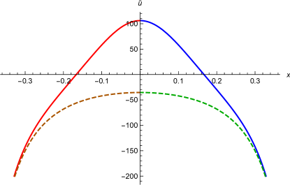
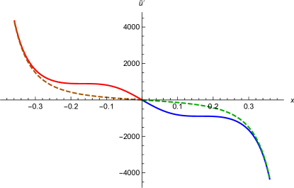
Figure 11: The solutions $x(\tilde{u})$, patching the two branches together at $x=0$, as well as its derivatives. In solid is the solution for ${\cal E}={\cal E}_{1}>0$, in dashed the solution for $\bar{\cal E}=-\bar{\cal E}_{1}<0$.

Note that this is an exact solution for a single source, but it also gives the leading behavior in case of several sources, especially how the non-trivial instanton-solution with two sources at $x=\pm 1/2$ can be regularized around its singularities.

Appendix B Finite-energy instanton solutions

We want to solve the instanton equation

$$\tilde{u}^{\prime\prime}(x)+\tilde{u}(x)^{2}=0\ .$$ (101)

Multiplying with $\tilde{u}^{\prime}(x)$ and integrating once gives

$$\frac{\tilde{u}^{\prime}(x)^{2}}{2}+\frac{\tilde{u}(x)^{3}}{3}=\cal E\ .$$ (102)

Solving for $\tilde{u}^{\prime}(x)$ yields

$$\tilde{u}^{\prime}(x)=\pm\sqrt{2{\cal E}-\textstyle\frac{2}{3}\tilde{u}(x)^{3}}\ ,$$ (103)

$$\frac{\tilde{u}^{\prime}(x)}{\sqrt{2{\cal E}-\textstyle\frac{2}{3}\tilde{u}(x)^{3}}}=\pm 1\ .$$ (104)

Integrating once, we find

$$\frac{\tilde{u}\,_{2}F_{1}\left(\frac{1}{3},\frac{1}{2};\frac{4}{3};\frac{\tilde{u}^{3}}{3\mathcal{E}}\right)}{\sqrt{2\mathcal{E}}}=\pm x+\mbox{const}\ .$$ (105)

These solutions are real for ${\cal E}>0$, which we consider first.

$$x_{\rm c}:=\lim_{u\to-\infty}\frac{\tilde{u}\,_{2}F_{1}\left(\frac{1}{3},\frac{1}{2};\frac{4}{3};\frac{\tilde{u}^{3}}{3\mathcal{E}}\right)}{\sqrt{2\mathcal{E}}}=-\frac{\sqrt[3]{3}\Gamma\left(\frac{1}{6}\right)\Gamma\left(\frac{4}{3}\right)}{\sqrt{2\pi}\sqrt[6]{\mathcal{E}}}\ .$$ (106)

The solution stops at last argument of the hypergeometric function being 1, i.e. $u=\sqrt[3]{3\cal E}$, s.t.

$$x_{0}:=\frac{\tilde{u}\,_{2}F_{1}\left(\frac{1}{3},\frac{1}{2};\frac{4}{3};\frac{\tilde{u}^{3}}{3\mathcal{E}}\right)}{\sqrt{2\mathcal{E}}}\Big{|}_{u\to\sqrt[3]{3\cal E}}=\frac{\sqrt[3]{3}\sqrt{\frac{\pi}{2}}\Gamma\left(\frac{4}{3}\right)}{\sqrt[6]{\mathcal{E}}\,\Gamma\left(\frac{5}{6}\right)}\ .$$ (107)

Note that $x_{\rm c}=-2x_{0}.$ This allows us to write a solution symmetric around $x=0$, (with the r.h.s. being positive)

$$\pm x=\frac{\sqrt[3]{3}\sqrt{\pi}\Gamma\left(\frac{4}{3}\right)}{\sqrt{2}\sqrt[6]{{\cal E}}\Gamma\left(\frac{5}{6}\right)}-\frac{\tilde{u}\,_{2}F_{1}\left(\frac{1}{3},\frac{1}{2};\frac{4}{3};\frac{\tilde{u}^{3}}{3{\cal E}}\right)}{\sqrt{2{\cal E}}}\ .$$ (108)

The instanton has extension 1 for

$${\cal E}_{1}:=\left(\frac{\sqrt[3]{3}\sqrt{2\pi}\Gamma(\frac{1}{3})}{\Gamma(\frac{5}{6})}\right)^{\!6}=\frac{52488\pi^{3}\Gamma\left(\frac{4}{3}\right)^{6}}{\Gamma\left(\frac{5}{6}\right)^{6}}\ .$$ (109)

This yields for the positive branch of the solution with extension 1

$$\pm x=\frac{1}{6}-\frac{{\tilde{u}}\,_{2}F_{1}\!\left(\frac{1}{3},\frac{1}{2};\frac{4}{3};\frac{{\tilde{u}}^{3}}{3{\cal E}_{1}}\right)}{\sqrt{2{\cal E}_{1}}}\ .$$ (110)

Now we consider solutions for $\bar{\cal E}:=-{\cal E}>0$. Using Pfaffian transformations for the hypergeometric function yields

$$\pm x=\frac{\sqrt{6}{\tilde{u}}\,_{2}F_{1}\left(\frac{1}{2},1;\frac{7}{6};\frac{3\bar{\cal E}}{{\tilde{u}}^{3}+3\bar{\cal E}}\right)}{\sqrt{-3\bar{\cal E}-{\tilde{u}}^{3}}}+\frac{\sqrt[3]{3}\sqrt{2\pi}\Gamma\left(\frac{7}{6}\right)}{\sqrt[6]{\bar{\cal E}}\Gamma\left(\frac{2}{3}\right)}\ .$$ (111)

Note that this solution is real; the shift brings the solution around $x=0$. It has extension 1 in $x$-direction for

$$\bar{\cal E}_{1}=\left[\frac{\sqrt{2\pi}\Gamma\left(\frac{1}{3}\right)}{\sqrt[6]{3}\Gamma\left(\frac{5}{6}\right)}\right]^{6}=\frac{8\pi^{3}\Gamma\left(\frac{1}{3}\right)^{6}}{3\Gamma\left(\frac{5}{6}\right)^{6}}\ .$$ (112)

There,

$$\pm x=\frac{\sqrt{6}{\tilde{u}}\,_{2}F_{1}\left(\frac{1}{2},1;\frac{7}{6};\frac{3\bar{\cal E}}{{\tilde{u}}^{3}+3\bar{\cal E}}\right)}{\sqrt{-3\bar{\cal E}-{\tilde{u}}^{3}}}+\frac{1}{2}\Bigg{|}_{\bar{\cal E}=\bar{\cal E}_{1}}\ .$$ (113)

As is easily checked numerically, it agrees with the solution (52) of DelormeLeDoussalWiese2016

$$\tilde{u}(x)=-6\,{\cal P}\left(x+1/2;g_{2}=0,g_{3}=\frac{\Gamma\left(\frac{1}{3}\right)^{18}}{(2\pi)^{6}}\right)\ .$$ (114)

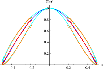
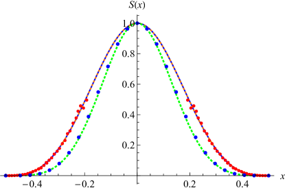
Figure 12: Left: Data reverse engineered from ThieryLeDoussalWiese2015 , slightly shifted in $x$-direction and rescaled in $y$-direction to collapse with our result for $S(x)$, normalized to 1. The exponents from top to bottom are $a=1/4$, $a=1/3$, and $a=1/2$. Contrary to the claims of ThieryLeDoussalWiese2015 , $a=1/4$ is not the best fit, but $a=1/3$, corresponding to a cubic behavior at the boundary. Right: Consistency with our theory (top curve). This is compared to the theory in ThieryLeDoussalWiese2015 and its numerical validiation: The lower dashed curve is the theory for avalanches with a large aspect ratio $S/\ell^{4}$ while the dots are the numerical verification from the same reference.

The function ${\cal P}$ is the Weierstrass $\cal P$-function. By construction, the solution $f(x)\equiv\tilde{u}(x)$ satisfies the following relations, which we give together for convenience:

$${f^{2}(x)+f^{\prime\prime}(x)=0}$$ (115)

$${\frac{2}{3}f^{3}(x)+f^{\prime}(x)^{2}=-36g_{3}\equiv-2{\bar{\cal E}_{1}}}$$ (117)

$${\frac{2}{3}f(x)f^{\prime\prime}(x)-f^{\prime}(x)^{2}=36g_{3}=2\bar{\cal E}_{1}}$$

Using these relations, some terms which in general are not total derivatives can be written as such, e.g.

$$f^{\prime}(x)^{2}=\frac{\mathrm{d}^{2}}{\mathrm{d}x^{2}}\left[\frac{1}{5}f(x)^{2}-\frac{3}{5}\overline{\cal E}_{1}x^{2}\right]\ .$$ (118)

Appendix C Reanalysis of the data of Ref. ThieryLeDoussalWiese2015

In Ref. ThieryLeDoussalWiese2015 it was claimed that when averaging over all avalanches of a given extension $\ell$, close to the boundary the scaling function grows as $\left<S(x)\right>_{\ell}\sim(x-\ell/2)^{4}$. This was supported by a log-log plot of the data, see figure 14 of Ref. ThieryLeDoussalWiese2015 . This procedure is dangerous, due to the boundary layer studied in section IV.3, which shifts the effective size of an avalanche. It is more robust to take $S(x)$ to the inverse expected power, and verify whether the resulting plot yields a straight line close to the boundary of the avalanche. This is done on Fig. 12. One clearly sees in the left plot that the data are most consistent with $a=\frac{1}{3}$, equivalent to a cubic growth close to the boundaries. We also show in the right of Fig. 12 that these data are consistent with our theory; note that the amplitude has been adjusted, since it could not be extracted from ThieryLeDoussalWiese2015 .

References

- (1) G. Durin and S. Zapperi, Scaling exponents for Barkhausen avalanches in polycrystalline and amorphous ferromagnets, Phys. Rev. Lett. 84 (2000) 4705–4708.
- (2) P. Le Doussal, K.J. Wiese, S. Moulinet and E. Rolley, Height fluctuations of a contact line: A direct measurement of the renormalized disorder correlator, EPL 87 (2009) 56001, arXiv:0904.1123.
- (3) D. Bonamy, L. Ponson, S. Prades, E. Bouchaud and C. Guillot, Scaling exponents for fracture surfaces in homogenous glass and glassy ceramics, Phys. Rev. Lett. 97 (2006) 135504.
- (4) H. Barkhausen, No Title, Phys. Z. 20 (1919) 401–403.
- (5) G. Durin and S. Zapperi, The Barkhausen effect, in G. Bertotti and I. Mayergoyz, editors, The Science of Hysteresis, page 51, Amsterdam, 2006, arXiv:0404512.
- (6) G. Durin, F. Bohn, M.A. Correa, R.L. Sommer, P. Le Doussal and K.J. Wiese, Quantitative scaling of magnetic avalanches, Phys. Rev. Lett. 117 (2016) 087201, arXiv:1601.01331.
- (7) A. Rosso, P. Le Doussal and K.J. Wiese, Avalanche-size distribution at the depinning transition: A numerical test of the theory, Phys. Rev. B 80 (2009) 144204, arXiv:0904.1123.
- (8) L.E. Aragon, A.B. Kolton, P. Le Doussal, K.J. Wiese and E. Jagla, Avalanches in tip-driven interfaces in random media, EPL 113 (2016) 10002, arXiv:1510.06795.
- (9) Ezequiel E. Ferrero, Laura Foini, Thierry Giamarchi, Alejandro B. Kolton and Alberto Rosso, Spatiotemporal patterns in ultraslow domain wall creep dynamics, Phys. Rev. Lett. 118 (2017) 147208.
- (10) A. Dobrinevski, P. Le Doussal and K.J. Wiese, Statistics of avalanches with relaxation and Barkhausen noise: A solvable model, Phys. Rev. E 88 (2013) 032106, arXiv:1304.7219.
- (11) Stefano Zapperi, Claudio Castellano, Francesca Colaiori and Gianfranco Durin, Signature of effective mass in crackling-noise asymmetry, Nat Phys 1 (2005) 46–49.
- (12) A. Dobrinevski, P. Le Doussal and K.J. Wiese, Avalanche shape and exponents beyond mean-field theory, EPL 108 (2014) 66002, arXiv:1407.7353.
- (13) L. Laurson, private communication.
- (14) L. Laurson, X. Illa, S. Santucci, K.T. Tallakstad, K.J. Måløy and M.J. Alava, Evolution of the average avalanche shape with the universality class, Nat. Commun. 4 (2013) 2927.
- (15) D.S. Fisher, Collective transport in random media: From superconductors to earthquakes, Phys. Rep. 301 (1998) 113–150.
- (16) K.J. Wiese and P. Le Doussal, Functional renormalization for disordered systems: Basic recipes and gourmet dishes, Markov Processes Relat. Fields 13 (2007) 777–818, cond-mat/0611346.
- (17) AA. Middleton, Asymptotic uniqueness of the sliding state for charge-density waves, Phys. Rev. Lett. 68 (1992) 670–673.
- (18) D.S. Fisher, Interface fluctuations in disordered systems: expansion, Phys. Rev. Lett. 56 (1986) 1964–97.
- (19) T. Nattermann, S. Stepanow, L.-H. Tang and H. Leschhorn, Dynamics of interface depinning in a disordered medium, J. Phys. II (France) 2 (1992) 1483–8.
- (20) O. Narayan and D.S. Fisher, Critical behavior of sliding charge-density waves in 4-epsilon dimensions, Phys. Rev. B 46 (1992) 11520–49.
- (21) P. Chauve, P. Le Doussal and K.J. Wiese, Renormalization of pinned elastic systems: How does it work beyond one loop?, Phys. Rev. Lett. 86 (2001) 1785–1788, cond-mat/0006056.
- (22) P. Le Doussal, K.J. Wiese and P. Chauve, 2-loop functional renormalization group analysis of the depinning transition, Phys. Rev. B 66 (2002) 174201, cond-mat/0205108.
- (23) P. Le Doussal, K.J. Wiese and P. Chauve, Functional renormalization group and the field theory of disordered elastic systems, Phys. Rev. E 69 (2004) 026112, cond-mat/0304614.
- (24) A.A. Middleton, P. Le Doussal and K.J. Wiese, Measuring functional renormalization group fixed-point functions for pinned manifolds, Phys. Rev. Lett. 98 (2007) 155701, cond-mat/0606160.
- (25) A. Rosso, P. Le Doussal and K.J. Wiese, Numerical calculation of the functional renormalization group fixed-point functions at the depinning transition, Phys. Rev. B 75 (2007) 220201, cond-mat/0610821.
- (26) P. Le Doussal and K.J. Wiese, Avalanche dynamics of elastic interfaces, Phys. Rev. E 88 (2013) 022106, arXiv:1302.4316.
- (27) P. Le Doussal and K.J. Wiese, Dynamics of avalanches, to be published (2011).
- (28) A. Dobrinevski, P. Le Doussal and K.J. Wiese, Non-stationary dynamics of the Alessandro-Beatrice-Bertotti-Montorsi model, Phys. Rev. E 85 (2012) 031105, arXiv:1112.6307.
- (29) P. Le Doussal and K.J. Wiese, First-principle derivation of static avalanche-size distribution, Phys. Rev. E 85 (2011) 061102, arXiv:1111.3172.
- (30) P. Le Doussal and K.J. Wiese, Elasticity of a contact-line and avalanche-size distribution at depinning, Phys. Rev. E 82 (2010) 011108, arXiv:0908.4001.
- (31) P. Le Doussal and K.J. Wiese, Size distributions of shocks and static avalanches from the functional renormalization group, Phys. Rev. E 79 (2009) 051106, arXiv:0812.1893.
- (32) P. Le Doussal, A.A. Middleton and K.J. Wiese, Statistics of static avalanches in a random pinning landscape, Phys. Rev. E 79 (2009) 050101 (R), arXiv:0803.1142.
- (33) A. Dobrinevski, Field theory of disordered systems – avalanches of an elastic interface in a random medium, arXiv:1312.7156 (2013).
- (34) T. Thiery, P. Le Doussal and K.J. Wiese, Spatial shape of avalanches in the Brownian force model, J. Stat. Mech. 2015 (2015) P08019, arXiv:1504.05342.
- (35) T. Thiery and P. Le Doussal, Universality in the mean spatial shape of avalanches, EPL 114 (2016) 36003, arXiv:1601.00174.
- (36) P. Le Doussal and K.J. Wiese, Distribution of velocities in an avalanche, EPL 97 (2012) 46004, arXiv:1104.2629.
- (37) M. Delorme, P. Le Doussal and K.J. Wiese, Distribution of joint local and total size and of extension for avalanches in the Brownian force model, Phys. Rev. E 93 (2016) 052142, arXiv:1601.04940.
- (38) I. Dornic, H. Chaté and M.A. Muñoz, Integration of Langevin equations with multiplicative noise and the viability of field theories for absorbing phase transitions, Phys. Rev. Lett. 94 (2005) 100601.