Cloak Imperfect: Impedance

Abstract

I investigate the scattering properties of transformation devices as the traditional impedance matching criteria are altered. This is demonstrated using simple theory and augmented by numerical simulations that investigate the role of impedance rescaling. Results are presented for transformation devices in a cylindrical geometry, but the lessons apply to both simpler and more complicated transformation devices. One technique used here is the use of impulsive field inputs, so that scattered fields are more easily distinguished from non-scattered fields.

I Introduction

Transformation Design – the use of the mathematical transformation of reference materials into those interesting “device” properties – is an area of active research interest. Investigations range all the way from the most abstract theory and conceptualizing Kinsler and McCall (2015a, 2014a); Smolyaninov (2013); Mackay and Lakhtakia (2011); Thompson et al. (2011) through to concrete theoretical proposals Pendry et al. (2006); Lai et al. (2009); Horsley et al. (2014); Mitchell-Thomas et al. (2013); Kinsler and McCall (2014b); McCall et al. (2011); McCall (2013) and technological implementations Schurig et al. (2006); Zhang et al. (2011); Frenzel et al. (2013); Lukens et al. (2014).

One aspiration is the “perfect cloak”, a Transformation Device (T-device) redirecting light, sound, or other signals so that a fixed interior (core) region is invisible and undetectable by outside observers. Although it seems that such a device is mathematically possible, there are many practical and technological constraints on what we can build that interfere with this ideal. Here I address the role of impedance rescaling, a common way of simplifying device designs.

As a start, it was noted that the original radial cloaking conception was impedance matched at the boundary Pendry et al. (2006). However, as far as standard impedance calculations are concerned, it was only impedance matched in the radial direction, and not in the angular or axial directions – but it is worth also noting that such naive uses of impedance measures in the anisotropic materials generated by transformation design schemes give misleading results McCall et al. (2016, ). In fact, interfaces between any medium and a transformed version (e.g. that subject to a linear scaling perpendicular to the interface) are guaranteed to be reflectionless.

Nevertheless, in the absence of a more general impedance calculation, I will still use it as a benchmark about which to consider impedance rescalings and their concomittant effect on scattering from a set of transformation devices. Here we will consider the simple example of a cylindrical transformation in a flat space, as used in many cloaking designs. The design is a purely spatial transformation applied to the EM constitutive parameters. As described in Kinsler and McCall (2015b) such a transformation changes the effective metric as seen by propagating electromagnetic fields. But, in changing the metric in order to “steer” the fields as demanded by the transformation, it does not specify anything about the impedance transformation. It is left as a side effect of the constitutive transformation, typically based on a “kappa medium” assumption where $\kappa=\epsilon=\mu$ (see e.g. McCall et al. (2016)), although other choices, such as assuming a dielectric-only response, are made depending on the situation or technological convenience.

One notable feature of many reported cloaking results, in either simulation or experiment, is that pictorial reprentations involve the steady state situation with an incident plane wave or other continuous wavefront. These usually show, as on fig. 1, a sufficiently convincing cloak performance, albeit with the kind of imperfections one might expect – such as a slightly modulated or attenuated wave pattern, providing evidence of scattering, absorption, or other imperfect implementation. However it is rarely clear what specific feature of the model gives rise to the imperfect performance. Notably, even numerical simulations are expected to have trouble near the singular material properties at core of a cloak, and we could well expect these to be the dominant source of error.

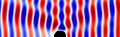
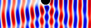
Figure 1: Finite difference time domain (FDTD) simulations of cloaking for plane wave (CW) sources on the left hand side. Results for two different cloaks, as described later in Sec. IV, are shown. The upper plot shows standard (linear) cloaking transformation, whereas the lower plot shows a smoother logarithmic cloaking transformation. Both show that the cloak functions as intended, albeit imperfectly; also that the differences between them are hard to discern by eye.

In this paper I investigate the role of impedance matching, as it is traditionally calculated, and how altered impedance choices affect the overall scattering performance. To do this I use snapshots from the impulsive probing of T-devices. This use of an impulse enables easy discrimination between scattering from the cloak halo and that from the core. This shows that although the core provides the dominant failing, the impedance matching also plays a role; a distinction important if one imagines probing a cloak with a beam that misses the core.

II Linear Rescaling Transformation

It is worthwhile considering a simple linear rescaling as a T-Design. Notably, a one-axis rescaling turns out to be a primitive building block for all T-devices. We can see why this is by considering two nearby regions in a T-device, which are infinitesimally different from one another as the properties of the transformation change with position. In order to maintain continuity of the transform over the contact surface between the two regions, they can only differ by a rescaling perpendicular to that surface. A two-axis linear rescaling cannot maintain continuity over a contact plane, only over the line along the unscaled axis.

As a result, at a sufficiently small scale, any transformation (or morphism) is reducible to single axis anisotropic scaling, although the orientation of that rescaling axis will typically vary with position.

Although this one axis rescaling has been treated previously McCall et al. (2016), I present an abbreviated version here. If the $x$ and $y$ directions are chosen parallel to the interface between two regions in a T-device, whether these have a finite or infinitesimal extent, we can rescale the $z$ axis in the second region by a factor $\lambda$. Thus the $z$-direction refractive index squared $n_{z}^{2}$ must change by $\lambda^{2}$, but the $x$ and $y$ direction counterparts ($n_{x}^{2}$ and $n_{y}^{2}$) remain unaltered.

Because EM is a transverse theory, this means that the $x$ and $y$ material responses are scaled by the transformations of the $z$ direction. If the first medium was isotropic with $\epsilon=\mu=\kappa_{1}$, the other is a new anisotropic “$\kappa_{\lambda}$” medium defined by

$$\kappa_{x}=\epsilon_{x}=\mu_{x} =\lambda\kappa_{1},$$ (1)

$$\kappa_{y}=\epsilon_{y}=\mu_{y} =\lambda\kappa_{1},$$ (2)

$$\kappa_{z}=\epsilon_{z}=\mu_{z} =\kappa_{1}.$$ (3)

The impedances also change, but of course there are two principal impedances per direction of propagation, each being the reciprocal of the other. The $z$ direction impedance squared is one of $Z_{z}^{2}=\left\{\mu_{x}/\epsilon_{y},\mu_{y}/\epsilon_{x}\right\}=1$; the $x$ direction impedance squared is one of $Z_{x}^{2}=\left\{\mu_{y}/\epsilon_{z},\mu_{z}/\epsilon_{y}\right\}=\left\{\lambda,\lambda^{-1}\right\}$; the $y$ direction impedance squared is one of $Z_{y}^{2}=\left\{\mu_{x}/\epsilon_{z},\mu_{z}/\epsilon_{x}\right\}=\left\{\lambda,\lambda^{-1}\right\}$.

Consequently, only rays (or waves) that cross between the two regions perpendicular to the interface see no calculated change in impedance; all others, to some extent, would be expected to probe the unmatched orientations. Although this leads to a natural assumption that there will then be scattering or reflection from the interface, in fact these calculated impedance mismatches do not result in reflections McCall et al. . This is a consequence of the fact that at least for EM, the usual transformation scheme preserves the solutions of Maxwell’s equations at the same time as it redistributes the propagation. This indicates that from a global perspective, scattering from the transformation-induced calculated impedance changes need not occur, even though from the traditional impedance perspective (e.g. Kinsler (2010)) it clearly must.

Figure 2: An interface between two (possibly infinitesimal) regions, with a change in scaling between the “ordinary” medium with properties given by $\kappa_{1}$, and the alternate medium which is scaled perpendicular to the interface by $\lambda$, with properties given by $\kappa_{\lambda}$.

III Radial Transformation Designs

Here we consider a 2D radial morphism where points with a laboratory or device coordinate $\hat{r}$ are transformed so as to appear at some apparent or design position $\tilde{r}=f(\hat{r})$, just as in the T-Design for a cylindrical cloak. Within this general approach, we can describe not only cloaks but also various types of illusion and/or distortion devices, and even two universes connected by a wormhole Gratus et al. (2017). However, we keep the mathematics general so that other non-cloak morphisms are allowed by the theory presented here. The original design for an electromagnetic cloak Pendry et al. (2006) used a transformation based on simple linear scaling of the radius, so here I will call that a linear-radial cloak. Other forms are possible, such as those based on polynomial forms (e.g. Cummer et al. (2009)) or the natural logarithm (see Cai et al. (2007); Kinsler and McCall (2015b) and later in this paper).

Here I will primarily consider three devices: (a) a radial distorter based on a piecewise linear transformation where objects in the core region will appear to an outside observer to have a smaller size (see fig. 3), (b) a smoothed radial distorter based on a cosine transformation, and (c) a smooth radial cloak based on a logarithmic transformation (see fig. 4).

Figure 3: Radial distorting device, with $\hat{r}$ to $\tilde{r}=f(\hat{r})$ mapping based on a piecewise linear scaling. We could turn this into a standard linear cloak by dropping $f(C)$ into the $\hat{r}$-axis, i.e. ensuring $f(C)=0$

Figure 4: Radial cloak based with an $\hat{r}$ to $\tilde{r}=f(\hat{r})=R\log_{10}(e\hat{r}/R)$ mapping based on the logarithmic function (as in Ma et al. (2009)). The core boundary is at $\hat{r}=R/e$, and the halo boundary – its interface with the exterior – is at $\hat{r}=R$.

Partly following Cummer et al. (2009), we define a radial transformation from device radial coordinate $\hat{r}$ to design (apparent) coordinate $\tilde{r}$:

$$\tilde{r} =f(\hat{r})$$ (4)

$$\textrm{with}\qquad f^{\prime}(\hat{r}) =\frac{\partial f(\hat{r})}{\partial\hat{r}}=\frac{\partial\tilde{r}}{\partial\hat{r}}$$ (5)

This means that

$$\kappa_{r}=\epsilon_{r}=\mu_{r} =\frac{f(\hat{r})}{\hat{r}f^{\prime}(\hat{r})},$$ (6)

$$\kappa_{\theta}=\epsilon_{\theta}=\mu_{\theta} =\frac{\hat{r}f^{\prime}(\hat{r})}{f(\hat{r})},$$ (7)

$$\kappa_{z}=\epsilon_{z}=\mu_{z} =\frac{f^{\prime}(\hat{r})f(\hat{r})}{\hat{r}}.$$ (8)

For a cloak, the finite radius $\hat{r}=C$ of the core region (in the laboratory) needs to behave as if contracted to the origin $\tilde{r}=f(\hat{r})=0$. This means that no matter what $f(\hat{r})$ we define, one of $\kappa_{r}$ or $\kappa_{\theta}$ will diverge near $\hat{r}=C$. Most likely this will be $\kappa_{\theta}$, since typically $f^{\prime}(\hat{r})$ will be finite, although if we engineered $f^{\prime}$ to vanish faster than $f(\hat{r})$ then $\kappa_{r}$ would diverge. The intermediate situation where $f^{\prime}\propto f$, which would allow non-singular properties, also means that $f$ is an exponential function, which has the wrong behaviour to be used for a cloak.

III.1 Index $n$

Given a T-Design defined by the function $\tilde{r}=f(\hat{r})$, we can directly find the material refractive indexes it needs to work. Assuming the design is to look like a space with fixed index normalized to $1$, they are

$$n_{r}^{2} =\left\{\epsilon_{\theta}\mu_{z},\epsilon_{z}\mu_{\theta}\right\}=\kappa_{\theta}\kappa_{z}=f^{\prime}(\hat{r})^{2}$$ (9)

$$n_{\theta}^{2} =\left\{\epsilon_{z}\mu_{r},\epsilon_{r}\mu_{z}\right\}=\kappa_{r}\kappa_{z}=\frac{f(\hat{r})^{2}}{\hat{r}^{2}}$$ (10)

$$n_{z}^{2} =\left\{\epsilon_{r}\mu_{\theta},\epsilon_{\theta}\mu_{r}\right\}=\kappa_{r}\kappa_{\theta}=1$$ (11)

The second term on each line indicates that there are two ways of making up each index from the underlying constitutive parameters (i.e. the permittivity and permeability). Typically we take this as an opportunity to restrict our design to only one of these polarizations, but for a perfect cloak both would have to be allowed for.

We see here that even for a cloak, it is trivial to ensure the index profiles are non singular, although $n_{\theta}$ does vanish on the inside core edge. It also looks relatively simple to index-match $n_{r}$ at the outer boundary by a suitable choice of gradient $f^{\prime}$, if there were a reason to do so. Note that the axial index $n_{z}$ is always the same as that of the background index.

III.2 Impedance $Z$

Now, based on the “standard” changes in $\epsilon$ and $\mu$ as specified in eqns. (6), (7), (8), we can calculate the impedances in the way they are usually defined. Each direction of propagation has an impedance that depends on the field polarization, and is derived from two principal values for that direction.

The radial impedance $Z_{r}$ has principal values which are

$$Z_{r}^{2} =\left\{\frac{\mu_{z}}{\epsilon_{\theta}},\frac{\mu_{\theta}}{\epsilon_{z}}\right\}=\left\{\frac{f(\hat{r})^{2}}{\hat{r}^{2}},\frac{\hat{r}^{2}}{f(\hat{r})^{2}}\right\}.$$ (12)

The radial impedance is therefore matched at the outer (halo) boundary where $R=f(R)$; note that this is true for any cloak, not just linear ones Pendry et al. (2006).

The angular impedance $Z_{\theta}$ has principal values which are

$$Z_{\theta}^{2} =\left\{\frac{\mu_{r}}{\epsilon_{z}},\frac{\mu_{z}}{\epsilon_{r}}\right\}=\left\{f^{\prime}(\hat{r})^{-2},f^{\prime}(\hat{r})^{2}\right\}.$$ (13)

Unlike the radial impedance, the angular impedance is not matched at the outer boundary unless our design is such that $f^{\prime}(R)=1$. Thus it is unmatched for the linear cloak – which was therefore not perfectly impedance matched, but is true for (e.g.) the logarithmic cloak.

The axial impedance $Z_{z}$ has principal values which are

$$Z_{z}^{2} =\left\{\frac{\mu_{\theta}}{\epsilon_{r}},\frac{\mu_{r}}{\epsilon_{\theta}}\right\}=\left\{\frac{r^{2}f^{\prime}(\hat{r})^{2}}{f(\hat{r})^{2}},\frac{f(\hat{r})^{2}}{\hat{r}^{2}f^{\prime}(\hat{r})^{2}}\right\}.$$ (14)

As for the radial impedance, the linear cloak again fails impedance matching, but if we have a design where $f^{\prime}(R)=1$ then it will be impedance matched at the outer boundary.

For a cloak, where $f(\hat{r})=0$ when $\hat{r}\neq 0$ at the core boundary, both $Z_{r}$ and $Z_{z}$ are zero or singular, depending on polarization. At the halo boundary $Z_{r}$ is unity (background), since $R=f(R)$, while the others depend on the gradient $f^{\prime}$. As long as the design ensures that $f^{\prime}(\hat{r})$ stays non-zero, the angular impedance need never be singular.

We might try to reduce the singularities in material properties at the core boundary by means of an $f(\hat{r})$ that skims at a vanishingly low angle into the $r$ axis, so that $f^{\prime}(\hat{r})\rightarrow 0$ (see e.g. Cummer et al. (2009)). Although this would be expected to reduce scattering by reducing the requirement for impractical material properties, this gain could well be balanced by an increase in impedance-derived scattering.

III.3 Transform $Z$ while preserving $n$

We now consider rescaling impedances by multiplying all permittivity values by a factor $\xi$ whilst dividing all permeability values by that same factor. The refractive indexes will then remain constant, preserving the cloak’s “steering” properties, but its impedance matching is altered.

For an electromagnetic cloak, we can choose to look mainly at the $r,\theta$ plane, and consider electric fields aligned only in the $r,z$ plane, so that only $\epsilon_{z}$, $\mu_{\theta}$, and $\mu_{r}$ are relevant. If we choose the factor $\xi=\hat{r}/f(\hat{r})$, then we can cancel the radial impedance profile inside the cloak. This makes the radial impedance have the same constant value inside the cloak as it has outside, and even a traditional interpretation would hold that no radially-travelling components would be reflected (scattered). However, this is at the cost of altering the variation in the angular profile $\bar{Z}_{\theta}^{2}$ which now depends on $f(\hat{r})$. Unfortnately, $f(\hat{r})$ causes problems, because it vanishes at $\hat{r}=C$. We find that

$$\bar{Z}_{r}^{2} =\frac{\bar{\mu}_{\theta}}{\bar{\epsilon}_{z}}=\frac{{\mu}_{\theta}/\xi}{{\xi\epsilon}_{z}}=\left[f^{\prime}\right]^{-1}.{f^{\prime}}=1,$$ (15)

$$\bar{Z}_{\theta}^{2} =\frac{\bar{\mu}_{r}}{\bar{\epsilon}_{z}}=\frac{{\mu}_{r}/\xi}{\xi{\epsilon}_{z}}=\left[\frac{f^{2}}{\hat{r}^{2}f^{\prime}}\right].{f^{\prime}}^{-1}=\frac{f^{2}}{\hat{r}^{2}f^{\prime 2}},$$ (16)

$$\bar{Z}_{z}^{2} =\frac{\bar{\mu}_{\theta}}{\bar{\epsilon}_{r}}=\frac{{\mu}_{\theta}/\xi}{\xi{\epsilon}_{r}}=\left[f^{\prime}\right].{f^{\prime}}={{f^{\prime}}^{2}}.$$ (17)

Here, for a cloak, none of the rescaled constitutive parameters need diverge near the core boundary, although $\bar{\mu}_{r}$ does tend to zero there.

Alternatively, by choosing $\xi=1/f^{\prime}(\hat{r})$ we can fix the angular impedance inside the cloak to be the same as that outside. However, the radial impedance is no longer matched at the halo boundary unless $f^{\prime}(b)=1$. We find that

$$\bar{Z}_{r}^{2} =\frac{\bar{\mu}_{\theta}}{\bar{\epsilon}_{z}}=\frac{{\mu}_{\theta}/\xi}{\xi{\epsilon}_{z}}=\left[\frac{\hat{r}{f^{\prime}}^{2}}{f}\right]^{-1}.\frac{f}{\hat{r}}=\frac{\hat{r}^{2}{f^{\prime}}^{2}}{f^{2}},$$ (18)

$$\bar{Z}_{\theta}^{2} =\frac{\bar{\mu}_{r}}{\bar{\epsilon}_{z}}=\frac{{\mu}_{r}/\xi}{\xi{\epsilon}_{z}}=\left[\frac{f}{\hat{r}}\right].\left(\frac{f}{\hat{r}}\right)^{-1}=1,$$ (19)

$$\bar{Z}_{z}^{2} =\frac{\bar{\mu}_{\theta}}{\bar{\epsilon}_{r}}=\frac{{\mu}_{\theta}/\xi}{\xi{\epsilon}_{r}}=\left[\frac{\hat{r}{f^{\prime}}^{2}}{f}\right].\left(\frac{f}{\hat{r}{f^{\prime}}^{2}}\right)^{-1}=\frac{\hat{r}^{2}{f^{\prime}}^{4}}{f^{2}}.$$ (20)

Here, for a cloak, we see that the $\bar{Z}_{r}$ and $\bar{Z}_{z}$ impedances are singular at the core boundary as a consequence of the rescaled constitutive parameters diverging or becoming zero.

Lastly, we might decide to fix the $z$ impedance inside the cloak to that outside. That is, we scale using $\xi=\hat{r}f^{\prime}/f$, so we find that

$$\bar{Z}_{r}^{2} =\frac{\bar{\mu}_{\theta}}{\bar{\epsilon}_{z}}=\frac{{\mu}_{\theta}/\xi}{\xi{\epsilon}_{z}}=\left[1\right].\left(\frac{{f^{\prime}}^{2}}{\hat{r}^{2}}\right)^{-1}=\frac{\hat{r}^{2}}{{f^{\prime}}^{2}}$$ (21)

$$\bar{Z}_{\theta}^{2} =\frac{\bar{\mu}_{r}}{\bar{\epsilon}_{z}}=\frac{{\mu}_{r}/\xi}{\xi{\epsilon}_{z}}=\left[\frac{f^{2}}{\hat{r}^{2}{f^{\prime}}^{2}}\right].\left(\frac{f^{2}}{\hat{r}^{2}}\right)^{-1}={f^{\prime}}^{-2}$$ (22)

$$\bar{Z}_{z}^{2} =\frac{\bar{\mu}_{\theta}}{\bar{\epsilon}_{r}}=\frac{{\mu}_{\theta}/\xi}{\xi{\epsilon}_{r}}=\left[1\right].1=1.$$ (23)

From this there are three distinct impedance rescalings that seem useful. We might continuously tune between the standard $\xi=1$ case with three parameters $a,b,c$, each adding in some degree those three cases discussed above. The combined scaling parameter is then $\xi=\xi_{r}\xi_{\theta}\xi_{z}$, where

1. $a$ scales towards the perfect radial $Z_{r}=1$ case by setting $\xi_{r}=(\hat{r}/f)^{a}$.

2. $b$ scales towards the perfect angular $Z_{\theta}=1$ case by setting $\xi_{\theta}=(1/f^{\prime})^{b}$.

3. $c$ scales towards the perfect axial $Z_{z}=1$ case by setting $\xi_{z}=(\hat{r}f^{\prime}/f)^{c}$.

From the above, we can see that the rescaling that fixes the radial impedance seems the best behaved: assuming $f^{\prime}$ is well behaved, the sole remaining difficulty is with the vanishing value of $\mu_{r}$ at the inner boundary. Also, any propagation along a predominantly angular path will be a mostly constant radius, and such propagation will not see any variation in impedances, which change only with radius.

IV Results

Although a perfectly implemented T-device should exhibit no unwanted scattering or reflections, we expect that one whose impedances have been rescaled as discussed in the preceeding section will do so. In such a case the traditional perspective, where impedance changes generate reflections and/or scattering again becomes relevant, and ensuring that there is no step-change along one given direction might have a trade-off involving the matching along other directions. Further, while asking for continuity in impedance is (was) usually the most important demand, impedance gradients would also be considered causes of reflections, albeit distributed ones that are likely to be weak.

To make these ideas about the effects of impedance matches, mismatches, and gradients more concrete I have performed sets of numerical simulations using MEEP Oskooi et al. (2010) for various impedance criteria. These were done in 2D (i.e. the $x,y$ plane), and for transverse electric fields $\bm{E}$, so that $E_{z}\neq 0$ but $H_{z}=0$. Further, although cloaking devices are typically more interesting than simple distorters of the type shown in fig. 3, they have singular material properties at their core boundary. Such singular properties give rise to numerical difficulties, and ones that potentially will obscure the impedance-based properties of interest here. Consequently I mainly show results for distorting devices, where it is easier to guarantee that the material properties are well behaved.

I consider two sample distorting functions, where $f_{i}(\hat{r})=\hat{r}+h_{i}(\hat{r})$. Both depend on a parameter $\alpha$, which specifies the (same) maximum displacement in either case. Further, it occurs at the same point $\hat{r}=R/2$ so that $h_{i}(R/2)=-\alpha R/2$. The functions $h_{i}(\hat{r})$ are

1. A piecewise linear distortion, where

   $$\qquad h_{1}(\hat{r}) =-\alpha\hat{r}; \textrm{for}\quad 0<\hat{r}\leq R/2$$ (24)

   $$\qquad h_{1}(\hat{r}) =\alpha\left(\hat{r}-R/2\right); \textrm{for}\quad R/2\geq\hat{r}<R.$$ (25)

   This is continuous, but does not match gradients. To ensure that $f(r)$ is single valued and always increasing, it requires $|\alpha|<1$.

2. A smoothly varying distortion, with

   $$h_{2}(\hat{r}) =\frac{\alpha R}{4}\left[\cos\left(\frac{2\pi\hat{r}}{R}\right)-1\right].$$ (26)

   This is both continuous and matches the gradient near the origin and at the boundary. Since

   $$h_{2}^{\prime}(\hat{r}) =\frac{\alpha\pi}{2}\sin\left(\frac{2\pi\hat{r}}{R}\right),$$ (27)

   we require that $\alpha<2/\pi$ to ensure that $f(\hat{r})$ is single valued and always increasing.

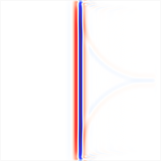
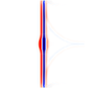
Figure 5: Comparison of electric field profiles $E_{z}$ taken when a planar wave packet, travelling from right to left, is half way across a piecewise linear distorting T-device with $\alpha=1/3$. To the left and right are the reference and distorting cases respectively; in the centre the difference between them, which also reveals the location of the T-device. The faint curved wavefronts trailing the main wave are artifacts of the source setup, but are shared by both reference and T-device simulations.

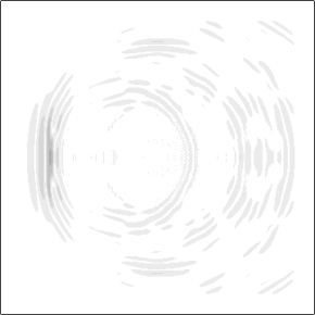
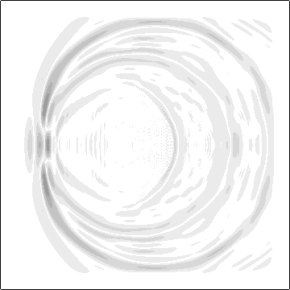
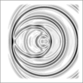
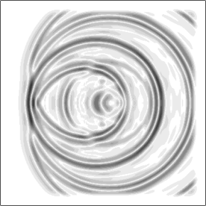
Figure 6: Net scattering $E_{z}-E_{0}$ from a piecewise linear non-cloaking transformation. A planar wave packet enters from the left hand side and traverses the distorting region in the centre. Because these plots only show the difference from the reference case, the wave packet is almost entirely cancelled out. However, if it were visible, it would form a vertical bar on the left hand side of each frame shown, coincident with the left-most scattered fields. The upper left frame shows the standard case, with a small amount of scattering; but since theoretically this design should be a perfect cloak, we can take this discrepancy to be an indication of the numerical error. The upper right frame shows the fixed matched radial impedance case. The lower frames show fixed matched angular impedance (left), and fixed matched axial impedance (right). The contrast ratio has been increased by a factor of $20$ over that for an ordinary non-difference plot.

The main quantity of interest here is the difference between a numerical simulation based on a T-device and another simulation based on the unremarkable design space the T-device is intended to mimic. In fig. 5 we can see such a comparison, depicted as a wave packet crossed the centre of a distorting T-device. However, the actual differences of interest are ones evaluated at a time after the input wave has passed through and then left the T-device, as well as after the bulk of the scattered waves have also departed it; but not before they reach the absorbing boundaries of the simulation edges.

However, before proceeding with more exhaustive comparisons, consider the scattering from the piecewise linear transformation above for different choices of impedance matching. This is shown pictorially in fig. 6 for four different cases, where the difference between the distorting simulation and a reference simulation with a homogeneous background material is taken. Since we choose a TE polarization for the simulations, the difference in the $z$ (axial) component of the electric fields is plotted. As discussed above, in each case the index profile of the material is the same, but different impedance criteria are imposed. Clearly the different cases give rise to different scattering levels.

In what follows we will combine the selected data from each specific simulation as shown pictorially in fig. 6 into a single numerical value representing the scattering induced by the distorting T-device. Each summed scattering value $S$ is calculated from the field values $E_{z}^{(i)}(x,y)$ and $E_{z}^{(0)}(x,y)$ for the distorting simulation and the reference simulation respectively. The calculation is

$$S^{(i)} =\int\int\left[E_{z}^{(i)}(x,y)-E_{z}^{(0)}(x,y)\right]^{2}dx~{}dy,$$ (28)

although below we will plot $\log_{10}(S)$ to enhance the level of detail visible on the figures. Note also that the $S$ values are unnormalised sums over the numerical data, and not corrected for (e.g.) simulation resolution.

Figure 7: Net numerical scattering vs distortion strength $\alpha$ for both linear ($+$) and smooth cosine ($\circ$) non-cloaking transformation, shown using a logarithmic scale. This is for the standard impedance $\kappa$ medium choice of $A=B=0$ .

In fig. 7 we can see how scattering increases for the standard impedance choice as the level of distortion is increased. If you take the position that in-principle transformation devices are capable of being perfect, as indicated by the lack of a reflection from a transformation-derived interface McCall et al. , then this figure provides a benchmark for the numerical error in the simulations.

The smooth cosine distortion usually gives less scattering, except as $\alpha$ approaches $1/2$, when its transform generates regions of extreme stretching (where $f^{\prime}(r)\rightarrow 0$). Although the piecewise linear distortion has the disadvantage of abrupt interfaces, the cosine distortion has regions that are more stretched, which can override the benefits of smoothness.

The next step is a more thorough search of the impedance rescaling parameter space for the two types of distorting T-device considered here. In the previous section, we said that if we take each of the “obvious” scalings in turn, each raised to some power $a$, $b$, and $c$, then the scaling factors will be $(\hat{r}/f)^{a}$, $(1/f^{\prime})^{b}$, or $(\hat{r}f^{\prime}/f)^{c}$. The net scaling in such a case is then $(\hat{r}/f)^{A}f^{\prime A-B}$ with $A=a+c$ and $B=b+a$. This means that instead of displaying a 3D dataset over the range of interesting $a,b,c$ it is sufficiently instructive to check just the 2D range $A,B$. Note that if $A=B$ then the scaling is $(\hat{r}/f)^{A}$, so that if $A=B=1$ then we have fixed the radial impedance at a fixed value which is impedance matched to the background space. If instead we choose $A=0$, then the scaling is $(1/f^{\prime})^{B}$, so that if $B=1$ we have fixed the angular impedance at a value impedance matched to the background space. Lastly, if $B=0$ then the scaling is $(\hat{r}f^{\prime}/f)^{A}$, so that at $A=1$ we have fixed the axial ($z$) impedance at a value impedance matched to the background space.

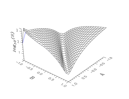
Figure 8: Net scattering $S$ vs impedance rescaling parameters $A,~{}B$ for a piecewise linear non-cloaking transformation, shown using a logarithmic scale. These results were obtained for a distortion strength of $\alpha=1/3$.

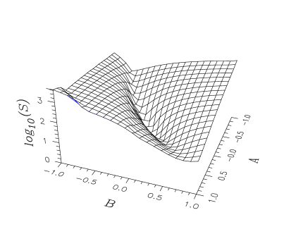
Figure 9: Net scattering $S$ vs impedance rescaling parameters $A,~{}B$ for the smooth cosine non-cloaking transformation, shown using a logarithmic scale. These results were obtained for a distortion strength of $\alpha=1/3$.

In figs. 8 and 9 we see the excess scattering of the two distorting T-devices. In both cases the best performance is at the standard case where $A=B=0$, with a slight degradation in performance away from the origin along the line $A=B$; and a strong degradation along $A=-B$.

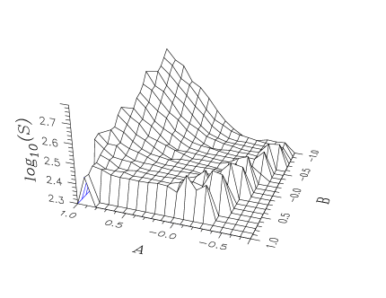
Figure 10: Net scattering $S$ vs impedance rescaling for the log-based cloaking transformation, shown using a logarithmic scale. In cases where the extreme material properties caused numerical difficulties, the $\log_{10}(S)$ values were set to the convenient value of +2.3 to aid presentation of the results.

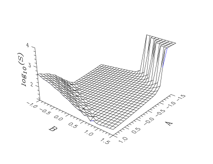
Figure 11: Net scattering $S$ vs impedance rescaling for the log-based cloaking transformation acting to shrink a metallic scatter, shown using a logarithmic scale. In the corner characterised by large negative $A$ and large positive $B$, the tendency for increased scattering is quickly overwhelmed by parameter ranges where the simulations become unreliable due to extreme material properties. Here the $\log_{10}(S)$ values were set to the convenient value of +4 in such cases.

It is also possible to do similar comparisons of cloaking T-devices rather that the distorting ones presented here. However, for both the linear cloaking transformation and a smoother logarithmic transformation, the scattering was dominated by the singular behaviour at the core boundary. Further, as can be seen in fig. 10, the impedance rescaling exacerbated numerical difficulties in some cases, so that a smaller range of rescalings gave useful results.

Therefore, in order to enable investigation of a wide parameter space, the cloak core was replaced with a larger metallic scatterer. The cloak transformation then acted simply to shrink the effective size of this scatterer. The comparison, then, is between the simulation of the cloak-based shrunk scatterer and a reference simulation with a scatter of the smaller (shrunken) size. For this case, only for larger values of $|A+B|$ could the impedance-induced scattering be seen over the other differences. See, for example, fig. 11, where the excess scattering is shown for a logarithmic cloaking function where $f(\hat{r})=R\log(e\hat{r}/R)$. Unlike the narrow valley features seen in fig. 8 and 9, the central part of the parameter space consists of a broad plateau. Note that due to the different simulation parameters, these cloaking-based $S$ values are not directly comparable to the distortion-based ones.

V Summary

Here we have seen that the usual $\epsilon=\mu$ transformation medium provides the best performance in numerical simulations, with a minimum of extraneous reflections and scattering from the boundary and interior of the transformed region. Although this result was to be expected, since on theoretical grounds the scattering should be exactly zero, a traditional optics view of impedance matching would not necessarily have supported such a conclusion. This is because, as shown here, a radial transformation such as that of the original Pendry et al. cylindrical cloak only matches – in the traditional sense – the radial impedance, with the angular and axial impedances left unmatched. Attempts to improve impedance matching (and so reduce scattering) by complementary rescalings of $\epsilon$ and $\mu$ were unsucessful; although not every possible rescaling was tested. It is therefore clear that the meaning of impedance is not well defined in the rather general types of anisotropic media that result from T-design.

One further conclusion that we can draw, is that it is important to be cautious when trying to improve on cloaking design, as in the scheme of Cummer et al. Cummer et al. (2009). Although such re-designs may remove or moderate singularities in material parameters, unless we can build the perfect $\epsilon=\mu$ device, the re-design may at the same time exacerbate impedance mismatches, leading to a scattering increase instead of the intended decrease. The use in this paper of an impulse wave profile to probe T-device performance was important in generating and understanding the results presented here – the scattered wave can be directly seen in pictorial plots, as well as after summation of the net scattering.