Resonant-tunneling
in discrete-time quantum walk

Abstract

We show that discrete-time quantum walks on the line, $\mathbb{Z}$, behave as “the quantum tunneling.” In particular, quantum walkers can tunnel through a double-well with the transmission probability $1$ under a mild condition. This is a property of quantum walks which cannot be seen on classical random walks, and is different from both linear spreadings and localizations.

Keywords quantum walk, quantum mechanics, resonant-tunneling, stationary measures.

1 Introduction

The quantum walk (QW) is a quantum version of the classical random walk. Their primitive forms of the discrete-time quantum walks on $\mathbb{Z}$ can be seen in Feynman’s checker board [1]. It is mathematically shown (e.g. [2]) that this quantum walk has a completely different limiting behavior from classical random walks, which is a typical example showing a difficulty of intuitive description of quantum walks’ behavior.

Relations between QW and its background quantum mechanics (QM) are very interesting, too. QW has been considered as quantum dynamical simulations such as, discretizations of the Dirac equation (e.g. [3, 4, 5]) and also spatially discretized Schrödinger equation (e.g. [6]). To connect QW to theses quantum dynamical system, some spatial and temporal scaling were needed to obtain the continuum limit from the discrete model of QW. However our model treated here reproduces naturally the following famous quantum dynamics model following the Schrödinger equation without any scaling limit. Here, we consider the quantum tunneling, which is one of the most famous quantum effects and has well-developed since the early period of QM; this effect shows that a quantum particle can tunnel through a barrier that it classically could not surmount (e.g. [7]). In particular, the resonant-tunneling [8, 9] is very impressive; consider the Schrödinger equation

$$i\frac{\partial}{\partial t}\psi(x,t)=-\frac{\partial^{2}}{\partial^{2}x}\psi(x,t)+V(x)\psi(x,t),\quad\psi(\cdot,t)\in C^{1}(\mathbb{R})$$

with a double-barrier (double-well) potential,

$$V(x)=\begin{cases}V_{0},&\mbox{ if }-L-w<x<-L\mbox{ or }L<x<L+w\\ 0,&\mbox{ otherwise. }\\ \end{cases}$$

Here, $2L>0$ is the distance between the two barriers, $w$ is the width of them, and $V_{0}>0$. Then, let us inject the the plane wave with positive energy $E$ from $x=-\infty$. The wave function $\psi(x,t)$ must be

$$\psi(x,t)=e^{-iEt}\times\begin{cases}e^{i\sqrt{E}x}+{\rho}e^{-i\sqrt{E}x},&\mbox{ for }x<-(L+w),\\ {\tau}e^{i\sqrt{E}x},&\mbox{ for }x>L+w,\\ \end{cases}$$

with constants $\tau$ and $\rho\in\mathbb{C}$. In this case, we define the transmission probability by $T=|{\tau}|^{2}$ and the reflection probability by $R=|{\rho}|^{2}$. It is well known that $T+R=1$. In particular, it holds that $T=1$ and $R=0$ for some resonance level, $E=E_{0}$. Therefore, the injected plane wave can tunnel the double-barrier without any reflection. Remark that $\psi$ is not a $L^{2}(\mathbb{R})$-function but a bounded function.

In this article, we show that the quantum walker can behave like the above resonant-tunneling. We consider a two-state QW on $\mathbb{Z}$ with two defects (double-barrier) and will prove that the quantum walker can tunnel through the double-barrier without any reflection, nevertheless the double-barrier has non-zero reflection elements. We call it Quantum resonant-tunneling walk (QRTW).

We believe that QRTW is the third  characteristic of QW compared to classical random walk, because any random walk on $\mathbb{Z}$ cannot archive $R=0$ except the trivial case and it is well-known that QW has (at least) two famous characteristics, namely, localization and linear spreading. The third interesting behavior cannot be derived without moving our concentration from the square summable space to the boundary functional space. From the view point of this $\ell^{\infty}$ space, our QW model describes the solution of the quantum graph [10, 11, 12] following the Schrödinger equation of the the quantum tunneling with double-barrier. See Section 3 for more detailed discussion.

Our organization of this paper is the following: In Section 2, we define our QW model with double-barrier and prove our main result, Theorem 2.2. In Section 3, we compare QRTW with resonant-tunneling in QM using quantum graph walk [11, 12]. In Section 4, we discuss our choice of initial states, stationary measures, and experimental realization. In Appendix, we give a short comment on the equality, $T+R=1$.

2 Main Theorem

Let us recall the definition of two-state QW model on $\mathbb{Z}$ (e.g. [13]). Define

$$|L\rangle=\begin{bmatrix}1\\ 0\end{bmatrix},\quad|R\rangle=\begin{bmatrix}0\\ 1\end{bmatrix},$$

where $L$ and $R$ refer to the left and right chirality state, respectively. The time evolution of the walk at $x\in\mathbb{Z}$ is determined by 2-dimensional unitary matrix

$$U_{x}=\begin{bmatrix}a_{x}&b_{x}\\ c_{x}&d_{x}\end{bmatrix}\in U(2).$$ (1)

To define the dynamics of our model, we divide $U_{x}$ into two matrices:

$$P_{x}=\begin{bmatrix}a_{x}&b_{x}\\ 0&0\end{bmatrix},\quad Q_{x}=\begin{bmatrix}0&0\\ c_{x}&d_{x}\end{bmatrix},$$

with $U_{x}=P_{x}+Q_{x}$. These $P_{x}$ and $Q_{x}$ represent that the walker moves to the left and the right at $x$ at each time step, respectively. Let $\Psi_{n}$ denote the amplitude at time $n$ of the QW on $\mathbb{Z}$:

$$\Psi_{n}=\begin{bmatrix}\cdots,\begin{bmatrix}\Psi_{n}^{L}(-1)\\ \Psi_{n}^{R}(-1)\\ \end{bmatrix},\begin{bmatrix}\Psi_{n}^{L}(0)\\ \Psi_{n}^{R}(0)\\ \end{bmatrix},\begin{bmatrix}\Psi_{n}^{L}(1)\\ \Psi_{n}^{R}(1)\\ \end{bmatrix},\cdots\end{bmatrix}^{\prime},$$

where $[\dots]^{\prime}$ denotes the transposed operation. Then the time evolution of the quantum walk is defined by

$$\Psi_{n+1}(x)=P_{x+1}\Psi_{n}(x+1)+Q_{x-1}\Psi_{n}(x-1),$$ (2)

where $\Psi_{n}(x)$ denotes the amplitude at time $n$ and position $x$. Equivalently,

$$\begin{bmatrix}\Psi_{n+1}^{L}(x)\\ \Psi_{n+1}^{R}(x)\end{bmatrix}=\begin{bmatrix}a_{x+1}\Psi_{n}^{L}(x+1)+b_{x+1}\Psi_{n}^{R}(x+1)\\ c_{x-1}\Psi_{n}^{L}(x-1)+d_{x-1}\Psi_{n}^{R}(x-1)\end{bmatrix}.$$

Let

$$\mathcal{H}:=\left\{\Psi=\{\Psi(x)\}_{x\in\mathbb{Z}};\|\Psi\|^{2}:=\sum_{x\in\mathbb{Z}}(|\Psi^{L}(x)|^{2}+|\Psi^{R}(x)|^{2})<\infty\right\}$$

be the total Hilbert space of our QW. It is well-known that (2) defines a unitary operator $U^{(s)}$ acting on $\mathcal{H}$ satisfying that

$$\Psi_{n}=(U^{(s)})^{n}\Psi_{0}$$

for any $n\geq 0$.

First, we consider the free case; namely,

$$U_{x}=\begin{bmatrix}e^{ip}&0\\ 0&e^{iq}\end{bmatrix}$$

with constants $p$ and $q\in\mathbb{R}$ for all $x\in\mathbb{Z}$. Let

$$\Psi_{0}(0)=\begin{bmatrix}0\\ 1\end{bmatrix},\quad\Psi_{0}(x)=\begin{bmatrix}0\\ 0\end{bmatrix}\quad(x\neq{0})$$

be an initial state $\Psi_{0}$. Then a quantum walker stays at $x=0$ at the initial time, and she, the quantum walker, moves to the position $x=n$ at the time $n$ with $\Psi_{n}(n)=\begin{bmatrix}0\\ e^{iqn}\end{bmatrix}.$ In contrast, if

$$\Psi_{0}(0)=\begin{bmatrix}1\\ 0\end{bmatrix},\quad\Psi_{0}(x)=\begin{bmatrix}0\\ 0\end{bmatrix}\quad(x\neq{0}),$$

she moves to the position $x=-n$ at the time $n$ with $\Psi_{n}(-n)=\begin{bmatrix}e^{ipn}\\ 0\end{bmatrix}$. These shows that the quantum walker freely runs over $\mathbb{Z}$.

In this article, we mainly consider the following QW with two defects at $x=0$ and $x=m(>0)$: let

$$U_{f}=\begin{bmatrix}e^{ip}&0\\ 0&e^{iq}\end{bmatrix},\quad U_{b}=\begin{bmatrix}a&b\\ c&d\end{bmatrix}\in U(2)$$

with constants $p$, $q\in\mathbb{R}$ and $a$, $b$, $c$, $d\in\mathbb{C}$, and

$$U_{x}=\begin{cases}U_{b},&\mbox{ if }x=0\mbox{ or }x=m,\\ U_{f},&\mbox{ otherwise. }\end{cases}$$

See Figure 1.

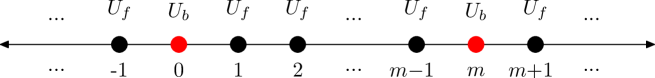
Figure 1: Two barriers $U_{b}$ are configured at $0$ and $m$.

Let

$$\Psi_{0}(x)=\begin{bmatrix}0\\ e^{iqx}\end{bmatrix}\mbox{ if }x<0,\quad\Psi_{0}(x)=\begin{bmatrix}0\\ 0\end{bmatrix}\mbox{ if }x\geq 0$$ (3)

be an initial state. Note that $\Psi_{0}\not\in\mathcal{H}$ but a bounded state and that $\Psi_{n}^{R}(x)$ is independent of $n$ for any $x<0$. In particular, $|\Psi_{n}^{R}(-1)|=1$, which means that one quantum walker moves into the left barrier at $x=0$ from $x=-1$ at each time step. This setting corresponds to inject a plane wave into the double-barrier from $x=-\infty$ in the resonant-tunneling situation of QM.

Consider the infinite time limit, that is, $n\to\infty$. Then we can expect that $(U^{(s)})^{n}\Psi_{0}$ converges to an $\ell^{\infty}$-stationary state $\Psi_{\infty}$ with

$$\Psi_{\infty}(x)=\begin{bmatrix}re^{ipx}\\ e^{iqx}\end{bmatrix}\mbox{ if }x<0,\quad\Psi_{\infty}(x)=\begin{bmatrix}0\\ te^{iqx}\end{bmatrix}\mbox{ if }x>m$$ (4)

with constants $r$ and $t\in\mathbb{C}$. We define the reflection probability $R=|r|^{2}$ and the transmission probability $T=|t|^{2}$. Note that $R+T=1$ (see Appendix). Here, we define that $\phi$ is an $\ell^{\infty}$-stationary state if and only if $\phi\in\ell^{\infty}(\mathbb{Z};\mathbb{C}^{2})$ and $\|((U^{(s)})^{n}\phi)(x)\|_{\mathbb{C}^{2}}^{2}=\|\phi(x)\|_{\mathbb{C}^{2}}^{2}$ for all $x\in\mathbb{Z}$ and $n\in\mathbb{N}$.

Our main interest is the following:

Do there exist $U_{f}$ and $U_{b}$ admitting that $T=1$ ?

If there are such operators $U_{f}$ and $U_{b}$, then (4) means that all quantum walkers tunnel through the double-barrier with probability $1$. This is a resonant-tunneling phenomenon of QW.

Remark 2.1.

The initial state $\Psi_{0}$ is not  in $\mathcal{H}$, but we apply $U^{(s)}$ to $\Psi_{0}$. Since we are interested in resonant-tunneling in QW, we must treat our problem in quantum scattering theory. (cf. The scattering state $\psi$ in QM in Section 1 is not a $L^{2}(\mathbb{R})$-function but a bounded function.) Therefore we extend the domain of $U^{(s)}$ to $\ell^{\infty}(\mathbb{Z})$ in a trivial way. See Section 4, too.

The following theorem is our main result in this article.

Theorem 2.2.

Assume that $\Phi(0)^{R}=1$ and $\Phi(x)^{L}=0$ for $x>m$. Let

$$r=\frac{be^{ip}(1+|U_{b}||U_{f}|^{m-1})}{1-bc|U_{f}|^{m-1}},\quad t=\frac{d^{2}e^{-2iq}}{1-bc|U_{f}|^{m-1}}$$ (5)

and

$$\tilde{r}=\frac{re^{-ip}-b}{a},\quad\tilde{t}=\dfrac{te^{iq(m+1)}}{d}.$$ (6)

Here, $|U_{f}|$ and $|U_{b}|$ denote the determinants of $U_{f}$ and $U_{b}$, respectively. Then we have that

$$U^{(s)}\Phi=\Phi\quad\iff\quad\Phi(x)=\begin{cases}\begin{bmatrix}re^{ipx}\\ e^{iqx}\end{bmatrix},&x\leq-1,\\ \\ \begin{bmatrix}\tilde{r}\\ 1\end{bmatrix},&x=0,\\ \\ \begin{bmatrix}\tilde{r}e^{ipx}\\ \tilde{t}e^{iq(x-m)}\end{bmatrix},&0<x<m,\\ \\ \begin{bmatrix}0\\ \tilde{t}\end{bmatrix},&x=m,\\ \\ \begin{bmatrix}0\\ te^{iqx}\end{bmatrix},&x\geq m+1.\\ \end{cases}$$ (7)

Proof.

Let us prove the necessary part. Since the quantum walker freely runs over $\mathbb{Z}\setminus\{0,m\}$ by $U_{f}$, we can write $\Phi(x)$ as in (7) at $x\in\mathbb{Z}\setminus\{0,m\}$. In addition, we have

$$\Phi(0)^{L}=\frac{\Phi(-1)^{L}-b\Phi(0)^{R}}{a}=\frac{re^{-ip}-b}{a}=\tilde{r}$$

and

$$\Phi(m)^{R}=\frac{\Phi(m+1)^{R}-c\Phi(m)^{L}}{d}=\frac{te^{iq(m+1)}}{d}=\tilde{t}.$$

Therefore, we have (6). Since $\Phi(1)^{R}=c\Phi(0)^{L}+d\Phi(0)^{R}=c\tilde{r}+d$, we have

$$\tilde{t}=\Phi(m)^{R}=e^{iq(m-1)}\Phi(1)^{R}=e^{iq(m-1)}[c\tilde{r}+d].$$

Similarly, since $\Phi(m-1)^{L}=a\Phi(m)^{L}+b\Phi(m)^{R}=b\tilde{t}$, we have

$$\tilde{r}=\Phi(0)^{L}=e^{ip(m-1)}\Phi(m-1)^{L}=be^{ip(m-1)}\tilde{t}.$$

Solving these simultaneous linear equations for $\tilde{t}$ and $\tilde{r}$, we obtain that

$$\begin{bmatrix}\tilde{t}\\ \tilde{r}\end{bmatrix}=\frac{de^{iq(m-1)}}{1-bc|U_{f}|^{m-1}}\begin{bmatrix}1\\ be^{ip(m-1)}\end{bmatrix}.$$

This and (6) imply (5). Checking $U^{(s)}\Phi=\Phi$ by direct computations, we can easily prove the sufficient part. ∎

Remark 2.3.

In this theorem, since we consider the situation where quantum walkers are constantly injected into the double-barrier from the left side, we assume that $\Phi(0)^{R}=1$ and $\Phi(x)^{L}=0$ for $x>m$. Let us consider the solution $\tilde{\Phi}$ of $U^{(s)}\tilde{\Phi}=\tilde{\Phi}$ with $\tilde{\Phi}(m)^{L}=1$ and $\tilde{\Phi}(x)^{R}=0$ for $x<0$. This solution $\tilde{\Phi}$ corresponds to the situation where quantum walkers are constantly injected into the double-barrier from the right  side. Then we can obtain all $\ell^{\infty}(\mathbb{Z})$-solutions of $U^{(s)}\Psi=\Psi$ by linear combinations of $\Phi$ and $\tilde{\Phi}$. N. Konno, et al, have studied such $\ell^{\infty}(\mathbb{Z})$-solutions in other contexts in [13, 14, 15, 16]. See Section 4, too.

This theorem gives us a mild condition for $T=1$, that is, QRTW. Note that the case where $b=c=0$ is trivial, because it is a reflection-less case. In the rest of this section, we omit this case.

Corollary 2.4.

Assume $bc\neq 0$. Then, we have $T=1\iff R=0\iff|U_{f}|^{m-1}|U_{b}|=-1$.

Proof.

QRTW is defined by $T=1$, equivalently, $R=0$. Since

$$R=|r|^{2}=\left|\frac{be^{ip}(1+|U_{b}||U_{f}|^{m-1})}{1-bc|U_{f}|^{m-1}}\right|^{2}$$

by Theorem 2.2, we obtain the desired result. ∎

Remark 2.5.

We can also prove this corollary using geometric series as follows.

Assume $|bc|=1$. Note that $a=d=0$ because $U_{b}$ is a unitary matrix. Therefore, any quantum walkers is completely reflected by the barriers. Thus, $T=0$.

Assume $|bc|<1$. Then $\Psi_{\infty}^{R}(m+1)={t}{}e^{iq(m+1)}$ is the summation of all the amplitudes of quantum walkers with $k$-times round trips between the two barriers. Since $\Psi_{n}^{R}(-1)=e^{-iq}$ for all $n$, we have

$$\Psi_{\infty}^{R}(m+1)=\sum_{k=0}^{\infty}d{e^{iq(m-1)}}\left[b{e^{ip(m-1)}}c{e^{iq(m-1)}}\right]^{k}d=\frac{e^{iq(m-1)}d^{2}}{1-bc|U_{f}|^{m-1}}.$$

Write the unitary matrix $U_{b}$ as

$$U_{b}=\begin{bmatrix}u\overline{\alpha}&u\overline{\beta}\\ v\beta&-v\alpha\end{bmatrix}\mbox{ with }\alpha,\beta,u,v\in\mathbb{C},|\alpha|^{2}+|\beta|^{2}=|u|=|v|=1$$

and put $e^{i\theta}=-|U_{f}|^{m-1}|U_{b}|$. Then, we have

$$\begin{split}|{t}|=\frac{1-|\beta|^{2}}{|1-e^{i\theta}|\beta|^{2}|}.\end{split}$$ (8)

Consequently, $T=|{t}|^{2}=1$ if and only if

$$1-2|\beta|^{2}+|\beta|^{4}=|1-e^{i\theta}|\beta|^{2}|^{2}=1-2|\beta|^{2}\cos\theta+|\beta|^{4}.$$

Thus we have $\beta=0$ or $\cos\theta=1$. Since the former is equivalent to $bc=0$, we can neglect this case by assumption. Since the latter is equivalent to $-|U_{f}|^{m-1}|U_{b}|=e^{i\theta}=1$, we obtain the desired result.

Corollary 2.6.

Let $I$ be the 2-dimensional identity matrix and $T_{\theta}=\begin{bmatrix}\cos 2\theta&\sin 2\theta\\ \sin 2\theta&-\cos 2\theta\end{bmatrix}$ with $\theta\in\mathbb{R}$. Take $U_{f}=I$ and $U_{b}=T_{\theta}$. Then, $T=1$.

This corollary is very important because $T_{\theta}$ corresponds to the Jones matrix of a half wave plate, which is used in the implementation of the discrete-time quantum walk by linear optical elements [17]. The detail of the implementation of QRTW will appear in our forthcoming article. Note that $T_{\theta}$ includes Hadamard matrix, $H=\dfrac{1}{\sqrt{2}}\begin{bmatrix}1&1\\ 1&-1\end{bmatrix}$, with $\theta=\pi/8$.

3 QRTW vs. Resonant-Tunneling in QM

In this section, we explain that our QRTW naturally connects the resonant-tunneling in QM in the limit of the double-barrier width is $0$, using the notion of the quantum graph [11, 12].

Let us consider the virtual quantum mechanical situation that delta potentials [10] are assigned on the real line $\mathbb{R}$ with the regular interval $s>0$ at $\{sj;\,j\in\mathbb{Z}\}$ and investigate the stationary behavior of the plane wave. We regard it as a “metric” graph whose vertices are the assigned delta potential’s places and the Euclidean length of edges are $s$. The height of the delta potential on $sj$ is described by $\alpha_{j}$ ($\geq 0$). Let $A$ be the set of symmetric directed edges of the one-dimensional lattice $A=\{(j,j+1),(j+1,j);\,j\in\mathbb{Z}\}$; in $A$, we distinguish the directed edge from $j$ to $j+1$ and that from $j+1$ to $j$, and each directed edge has the Euclidean length $s$. If $a=(i,j)\in A$, then the inverse directed edge is denoted by $\bar{a}$ and the origin and terminal vertices of $a$ are denoted by $o(a):=i$, $t(a):=j$, respectively. The problem can be converted to the quantum graph on this metric graph which describes the stationary state of the plane wave on all metric directed edges with the boundary conditions at each vertex: firstly, the domain of the wave function is the pair of directed edge $a\in A$ and the distance $x\in[0,s]$ from the origin vertex $o(a)$ satisfying $\varphi(a;x)=\varphi(\bar{a};s-x)$, that is,

$$\varphi\in\{\psi:A\times[0,s]\to\mathbb{C}\;|\;\psi(a;x)=\psi(\bar{a};s-x)\};$$ (9)

secondly, the stationary Schrödinger equation on each directed edge is

$$-\frac{d^{2}}{dx^{2}}\varphi(a;x)=k^{2}\varphi(a;x);$$ (10)

thirdly, the boundary conditions at each vertex $u$ are given by

$$\begin{split}&\varphi(a;0)=\phi_{u}\mathrm{\;for\;any\;}a\in A\mathrm{\;with\;}o(a)=u;\\ &\sum_{o(a)=u}\varphi^{\prime}(a;x)|_{x=0}=\alpha_{j}\phi_{u},\end{split}$$ (11)

where $\phi_{u}\in\mathbb{C}$ is an independent value of the connected directed edge, and $\varphi^{\prime}$ is the derivative of $\varphi$ with respect to $x\in[0,s]$. From (9) and (10), $\varphi(a;x)$ is described by using some complex values $\{\gamma_{a}\}_{a\in A}$ as follows:

$$\varphi(a;x)=\gamma_{a}e^{-ikx}+\gamma_{\bar{a}}e^{-ik(s-x)}.$$ (12)

Thus the problem is further reduced to find $\gamma_{a}$’s satisfying the boundary conditions (11). The solution $\{\gamma_{a}\}_{a\in A}$ satisfying all the boundary conditions (11) on all the vertices connects a quantum walk as follows.

Proposition 3.1 ([18]).

Let $U_{j}$ be the $2$-dimensional unitary matrix of the quantum walk on $\mathbb{Z}$ $(j\in\mathbb{Z})$ in (1) whose elements are given by

$$a_{j}=d_{j}=\frac{2e^{iks}}{2+i\alpha_{j}/k},\quad b_{j}=c_{j}=e^{iks}\left(\frac{2}{2+i\alpha_{j}/k}-1\right),$$

and $U^{(s)}$ be the total unitary operator of the quantum walk. Then $\{\gamma_{a}\}_{a\in A}$ in (12) is the solution satisfying the boundary conditions (11) for all $u\in V$ if and only if

$$U^{(s)}\Psi=\Psi,$$

where $\Psi(j)=[\gamma_{a},\gamma_{b}]^{\prime}$ with $t(a)=t(b)=j$ and $o(a)=j+1$, $o(b)=j-1$.

Therefore the setting below of the following delta potential provides the corresponding quantum tunneling walk:

$$\alpha_{j}=\begin{cases}\alpha:=wV_{0}&\text{: $j=0,m$;}\\ 0&\text{: otherwise.}\end{cases}$$

Note the well known fact that the barrier potential with the width $w$ and the height $V_{0}$ (as in Section 1) converges to the delta potential $\alpha\delta(x)$ with $\alpha=wV_{0}$ as $w\downarrow 0$ [10]. Thanks to Theorem 2.2, the solution $\{\gamma_{a}\}_{a\in A}$ can be explicitly obtained. Thus the stationary state of our quantum tunneling walk in $\ell^{\infty}$ is not only isomorphic to the stationary solution of the quantum graph corresponding to the double-barrier delta potentials but also able to provide the solution explicitly. Using this, for example, we can compute the transmission probability $T$ of the quantum graph by

$$T=|t|^{2}=\left(\frac{1-\frac{(\alpha/k)^{2}}{4+(\alpha/k)^{2}}}{\left|1+e^{2iksm}\frac{2-i\alpha/k}{2+i\alpha/k}\frac{(\alpha/k)^{2}}{4+(\alpha/k)^{2}}\right|}\right)^{2}=\left(\frac{1-|\beta|^{2}}{|1-e^{i\theta}|\beta|^{2}|}\right)^{2}$$ (13)

with $|\beta|^{2}=\frac{4}{4+(\alpha/k)^{2}}$ and $e^{i\theta}=-e^{2iksm}\frac{2-i\alpha/k}{2+i\alpha/k}$. Therefore, we can obtain that

$$T=1\iff e^{2iksm}\frac{2-i\alpha/k}{2+i\alpha/k}=-1$$ (14)

in the way similar to Remark 2.5. We can easily check that (14) is consistent with Corollary 2.4. Figure 2 shows the dependence of the transmission probability $T$ on the wave number $k$ obtained by our quantum tunneling walk which is a famous figure known as showing the quantum perfect transmission with the double-barrier, e.g., [10].

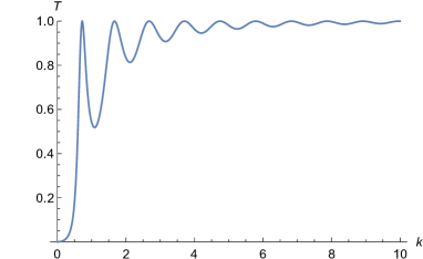
Figure 2: The wave number $k$ vs. the transmission probability $T$ in (13) of the quantum graph for the $\alpha=1$ and $sm=3$ case: the wave numbers where the perfect transmission exhibits satisfy (14).

4 Discussion

Our $\ell^{\infty}(\mathbb{Z})$-category investigations of QW in this article have established the relation between QW and quantum scattering theory and, in particular, revealed a resonant-tunneling phenomenon of QW.

As already mentioned, the limit state $\Psi_{\infty}$ satisfies $U^{(s)}\Psi_{\infty}=\Psi_{\infty}$ and $\Psi_{\infty}\in\ell^{\infty}(\mathbb{Z})$. Though we have considered the initial state $\Psi_{0}$ defined by (3) in Section 2 for simplicity, it is natural to take another initial state,

$$\Phi_{0}(x)=\begin{bmatrix}0\\ e^{i(q+\delta)x}\end{bmatrix}\mbox{ if }x<0,\quad\Phi_{0}(x)=\begin{bmatrix}0\\ 0\end{bmatrix}\mbox{ if }x\geq 0,$$

where $\delta\in\mathbb{R}$. We can treat it in a same way as in Section 2. Each amplitude of $\Phi_{0}(x)$ gains a phase shift $e^{i\delta}$ at each time step. Therefore, the infinite time limit $\Phi_{\infty}$ satisfies $U^{(s)}\Phi_{\infty}=e^{i\delta}\Phi_{\infty}$. In addition, since

$$\Phi_{\infty}^{R}(m+1)=\frac{e^{iq(m-1)}d^{2}}{1-e^{i\delta(m-1)}|U_{f}|^{m-1}bc},$$

we have that $T=1$ if and only if $(e^{i\delta}|U_{f}|)^{m-1}|U_{b}|=-1$ and $|bc|<1$.

In general, if there exists an eigenfunction $\Psi$ of $U^{(s)}$ in $\ell^{\infty}(\mathbb{Z})$, then we can define a stationary measure of the QW at position $x\in\mathbb{Z}$ by

$$\mu(x)=|\Psi^{L}(x)|^{2}+|\Psi^{R}(x)|^{2}.$$

N. Konno, et al, have comprehensively studied such measures [13, 14, 15, 16].

The authors consider that such $\ell^{\infty}$-category studies will be important in various areas of study of QW.

Finally, we mention that this resonant-tunneling phenomenon of QW can be realized in experiment. The operators will be implemented by half wave plates and polarizing beam splitters, and the steady injection of the quantum walker will be implemented by laser. The conceptual design of ring-resonator named Quantum Walk Resonator will be discussed in the forthcoming paper.

Appendix

We use the fact that $R+T=1$ without any proof, because this is an elementary fact derived from the two facts, the unitarity of $U^{(s)}$ and $\Psi_{\infty}$ being a stationary state; that is, $U^{(s)}\Psi_{\infty}=\Psi_{\infty}$. Consider the inflow and outflow of $\Psi_{\infty}$ with respect to the interval $I:-1\leq{x}\leq{m+1}$. The quantity,

$$P(\Psi_{\infty};I)=\sum_{x=-1}^{m+1}(|\Psi_{\infty}^{L}(x)|^{2}+|\Psi_{\infty}^{R}(x)|^{2}),$$

is the relative existence probability of quantum walkers in $I$. Since $\Psi_{\infty}$ is stationary, $P(\Psi_{\infty};I)$ is independent of time. On the other hand, since $U_{-3}=U_{-1}=U_{m+1}=U_{m+3}=U_{f}$, we have that $|\Psi_{\infty}^{R}(-2)|^{2}+|\Psi_{\infty}^{L}(m+2)|^{2}$ and $|\Psi_{\infty}^{L}(-2)|^{2}+|\Psi_{\infty}^{R}(m+2)|^{2}$ are the inflow and outflow of $I$, respectively. Consequently, these two quantities must be equal to each other. The former is $1+0=1$ by the definition of $\Psi_{\infty}$ and the latter is $|{r}|^{2}+|{t}|^{2}=R+T$. Therefore, $R+T=1$. Note that this argument is valid even if there are more than two barriers $U_{b}$ in $I$.

References

• [1] R. P. Feynman, A. R. Hibbs., Quantum mechanics and path integrals, Dover Publications, Inc., Mineola, NY, emended edition, 2010.
• [2] N. Konno., Quantum random walks in one dimension, Quantum Information Processing 1(5) 345–354, 2002.
• [3] F. W. Strauch., Discrete-time quantum walks: Continuous limit and symmetries, J. Math. Phys. 48, 082102, 2007.
• [4] G. D. Molfetta, F. Debbasch., Discrete-time quantum walks: continuous limit and symmetries, Journal of Mathematical Physics 53, 123302, 2012
• [5] P. Arrighi, V. Nesme and M. Forets., The Dirac equation as a quantum walk: higher dimensions, observational convergence J. Phys. A: Math. Theor. 47 465302, 2014
• [6] Y. Shikano, From Discrete Time Quantum Walk to Continuous Time Quantum Walk in Limit Distribution, J. Comput. Theor. Nanosci. 10, 1558-1570, 2013.
• [7] A. Messiah., Quantum Mechanics Volume 1, North-Holland, Amsterdam, 1961.
• [8] R. Tsu, L. Esaki., Tunneling in a finite superlattice, Appl. Phys. Lett. 22, 562–564, 1973; doi:10.1063/1.1654509.
• [9] L. L. Chang, L. Esaki, R. Tsu., Resonant tunneling in semiconductor double barriers, Appl. Phys. Lett. 24, 593–595, 1974; doi:10.1063/1.1655067.
• [10] S. Albeverio, F. Gesztesy, R. Høegh-Krohn, H. Holden, P. Exner., Solvable Model in Quantum Mechanics, AMS Chelsea publishing, 2004.
• [11] P. Exner, P. Seba., Free quantum motion on a branching graph, Rep. Math. Phys. 28, 7–26, 1989.
• [12] S. Gnutzmann, U. Smilansky., Quantum graphs: Applications to quantum chaos and universal spectral statistics, Advances in Physics, 55, 527–625, 2006.
• [13] N. Konno, M. Takei., The non-uniform stationary measure for discrete-time quantum walks in one dimension, Quantum Inf. Comput. 15, 1060–1075, 2015.
• [14] T. Endo, N. Konno., The stationary measure of a space-inhomogeneous quantum walk on the line, Yokohama Math. J. 60, 33–47, 2014.
• [15] T. Endo, H. Kawai, N. Konno., Stationary measures for the three-state Grover walk with one defect in one dimension, 2016; arXiv:1608.07402.
• [16] H. Kawai, T. Komatsu, N. Konno., Stationary measure for two-state space-inhomogeneous quantum walk in one dimension, 2017; arXiv:1707.04040.
• [17] Z. Zhao, J. Du, H. Li, T. Yang, Z.-B. Chen, J.-W. Pan, Implement quantum random walks with linear optics elements, 2002; arXiv:quant-ph/0212149.
• [18] Yu. Higuchi, N. Konno, I. Sato, E. Segawa., Quantum graph walk I: mapping to quantum walks, Yokohama  Mathematical  Journal 59, 33-55, 2013.