Hard photoproduction of a diphoton with a large invariant mass

Abstract

The electromagnetic probe has proven to be a very efficient way to access the $3-$dimensional structure of the nucleon, particularly thanks to the exclusive Compton processes. We explore the hard photoproduction of a large invariant mass diphoton in the kinematical regime where the diphoton is nearly forward and its invariant mass is the hard scale enabling to factorize the scattering amplitude in terms of generalized parton distributions. This amplitude has a very peculiar and interesting analytic structure. We calculate unpolarized cross sections and the angular asymmetry triggered by a linearly polarized photon beam.

I Introduction

The last twenty years have witnessed a tremendous progress in the understanding of hard exclusive scattering in the framework of the QCD collinear factorization of hard amplitudes in specific kinematics in terms of generalized parton distributions (GPDs) and hard perturbatively calculable coefficient functions historyofDVCS ; gpdrev .

In this paper, we study the exclusive photoproduction of two photons on a unpolarized proton or neutron target

$$\gamma(q,\epsilon)+N(p_{1},s_{1})\rightarrow\gamma(k_{1},\epsilon_{1})+\gamma(k_{2},\epsilon_{2})+N^{\prime}(p_{2},s_{2})\,,$$ (1)

in the kinematical regime of large invariant diphoton mass $M_{\gamma\gamma}$ of the final photon pair and small momentum transfer $t=(p_{2}-p_{1})^{2}$ between the initial and the final nucleons. Roughly speaking, these kinematics means a moderate to large, and approximately opposite, transverse momentum of each final photon. This reaction has a number of interesting features. First, it is a purely electromagnetic process at Born order - as are deep inelastic scattering (DIS), deeply virtual Compton scattering (DVCS) and timelike Compton scattering (TCS) - and, although there is no deep understanding of this fact, this property is usually accompanied by early scaling. Second, the process is insensitive to gluon GPDs because of the charge symmetry of the two photon final state. This may help to reduce QCD next to leading order corrections (which we do not calculate here) since they are often more important for gluon initiated partonic processes than for quark initiated ones. Third, there is also no contribution from the badly known chiral-odd quark distributions. This study enlarges the range of $2\to 3$ reactions analyzed in the framework of collinear QCD factorization 2to3 ; elb .

II Kinematics

Let us first present the kinematics of the process (1). We decompose every momenta on a Sudakov basis as

$$v^{\mu}=a\,n^{\mu}+b\,p^{\mu}+v_{\bot}^{\mu}\,,$$ (2)

with $p$ and $n$ the light-cone vectors

$$p^{\mu}=\frac{\sqrt{s}}{2}(1,0,0,1)\,,\qquad n^{\mu}=\frac{\sqrt{s}}{2}(1,0,0,-1)\,,\qquad p\cdot n=\frac{s}{2}\,,$$ (3)

and

$$v^{+}=v.n\,,\qquad v_{\bot}^{\mu}=(0,v^{x},v^{y},0)\,,\qquad v_{\bot}^{2}=-\vec{v}_{t}^{2}\,.$$ (4)

The particle momenta read

$$p_{1}^{\mu} = (1+\xi)\,p^{\mu}+\frac{M^{2}}{s(1+\xi)}\,n^{\mu}~{},\quad p_{2}^{\mu}=(1-\xi)\,p^{\mu}+\frac{M^{2}+\vec{\Delta}^{2}_{t}}{s(1-\xi)}n^{\mu}+\Delta^{\mu}_{\bot}\,,\quad q^{\mu}=n^{\mu}~{},$$

$$k_{1}^{\mu} = \alpha_{1}\,n^{\mu}+\frac{(\vec{p}_{t}-\vec{\Delta}_{t}/2)^{2}}{\alpha_{1}s}\,p^{\mu}+p_{\bot}^{\mu}-\frac{\Delta^{\mu}_{\bot}}{2}~{},~{}~{}k_{2}^{\mu}=\alpha_{2}\,n^{\mu}+\frac{(\vec{p}_{t}+\vec{\Delta}_{t}/2)^{2}}{\alpha_{2}s}\,p^{\mu}-p_{\bot}^{\mu}-\frac{\Delta^{\mu}_{\bot}}{2}\,,$$ (5)

where $M$ is the mass of the nucleon and $\xi$ is the skewness parameter. We define $\Delta^{\mu}=p_{2}^{\mu}-p_{1}^{\mu}$ and $P^{\mu}=\frac{1}{2}(p_{1}^{\mu}+p_{2}^{\mu})$.

The total center-of-mass energy squared of the $\gamma$-N system is

$$S_{\gamma N}=(q+p_{1})^{2}=(1+\xi)s+M^{2}\,.$$ (6)

The Mandelstam invariants read

$$t = (p_{2}-p_{1})^{2}=-\frac{1+\xi}{1-\xi}\vec{\Delta}_{t}^{2}-\frac{4\xi^{2}M^{2}}{1-\xi^{2}}\,,$$ (7)

$$M_{\gamma\gamma}^{2} = ~{}(k_{1}+k_{2})^{2}=~{}2\xi\,s\left(1-\frac{2\,\xi\,M^{2}}{s(1-\xi^{2})}\right)-\vec{\Delta}_{t}^{2}\frac{1+\xi}{1-\xi}\,,$$ (8)

$$-t^{\prime} = -(k-q)^{2}=~{}\frac{(\vec{p}_{t}-\vec{\Delta}_{t}/2)^{2}}{\alpha_{1}}\;,$$ (9)

$$-u^{\prime} = -(k_{2}-q)^{2}=~{}\frac{(\vec{p}_{t}+\vec{\Delta}_{t}/2)^{2}}{\alpha_{2}}\;.$$ (10)

The simplified kinematical relations used to calculate the hard coefficient functions are :

$$\alpha_{1}+\alpha_{2}=1~{}~{}~{}~{},~{}~{}~{}~{}\alpha_{1}\alpha_{2}=\frac{\vec{p_{t}}^{2}}{M^{2}_{\gamma\gamma}}~{}~{}~{}~{},~{}~{}~{}~{}\xi=\frac{\tau}{2-\tau}~{}~{}~{}~{},~{}~{}~{}~{}\tau=\frac{M^{2}_{\gamma\gamma}-t}{S_{\gamma N}-M^{2}}\,.$$ (11)

III The scattering amplitude

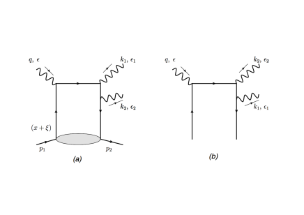
Figure 1: Feynman diagrams contributing to the coefficient functions of the process $\gamma N\to\gamma\gamma N^{\prime}$

Factorization allows to write the scattering amplitude as

$$\mathcal{T} =\frac{1}{4}\int_{-1}^{1}dx\sum_{q}\int dz^{-}\exp(ixz^{-}P^{+})\left\langle p_{2},s_{2}\left|\overline{\psi}_{q}\left(-\frac{z}{2}\right)\left[CF^{V}_{q}\not{n}+CF^{A}_{q}\not{n}\gamma^{5}\right]\psi_{q}\left(\frac{z}{2}\right)\right|p_{1},s_{1}\right\rangle$$ (13)

$$=\frac{1}{2}\;\frac{1}{2P^{+}}\int_{-1}^{1}dx\sum_{q}\left[CF^{V}_{q}(x,\xi)\left(H^{q}(x,\xi)\bar{U}(p_{2},s_{2})\not{n}U(p_{1},s_{1})+E^{q}(x,\xi)\bar{U}(p_{2},s_{2})\frac{i\sigma^{\mu\nu}\Delta_{\nu}n_{\mu}}{2M}U(p_{1},s_{1})\right)+\right.$$

$$\left.~{}~{}~{}~{}~{}~{}~{}~{}~{}~{}~{}~{}~{}~{}~{}~{}~{}~{}~{}~{}~{}+CF^{A}_{q}(x,\xi)\left(\tilde{H}^{q}(x,\xi)\bar{U}(p_{2},s_{2})\not{n}\gamma^{5}U(p_{1},s_{1})+\tilde{E}^{q}(x,\xi)\bar{U}(p_{2},s_{2})\frac{i\gamma_{5}(\Delta\cdot n)}{2M}U(p_{1},s_{1})\right)\right]\,,$$

with the coefficient functions calculated from the diagrams of Fig. 1 as

$$iCF^{V}_{q} = Tr[i\mathcal{M}\not p]=-ie_{q}^{3}\left[A^{V}\left(\frac{1}{D_{1}(x)D_{2}(x)}+\frac{1}{D_{1}(-x)D_{2}(-x)}\right)+\right.$$

$$B^{V}\left(\frac{1}{D_{1}(x)D_{3}(x)}+\frac{1}{D_{1}(-x)D_{3}(-x)}\right)+\left.C^{V}\left(\frac{1}{D_{2}(x)D_{3}(-x)}+\frac{1}{D_{2}(-x)D_{3}(x)}\right)\right]\,,$$

$$iCF^{A}_{q} = Tr[i\mathcal{M}\gamma^{5}\not p]=-ie_{q}^{3}\left[A^{A}\left(\frac{1}{D_{1}(x)D_{2}(x)}-\frac{1}{D_{1}(-x)D_{2}(-x)}\right)+\right.\left.B^{A}\left(\frac{1}{D_{1}(x)D_{3}(x)}-\frac{1}{D_{1}(-x)D_{3}(-x)}\right)\right]$$

where ${\mathcal{M}}\not p$ and ${\mathcal{M}}\gamma^{5}\not p$ are contributions of the hard part of scattering amplitude projected on vector and axial vector Fierz structures, $e_{q}=Q_{q}|e|$ and the denominators read

$$D_{1}(x)=s(x+\xi+i\varepsilon)~{}~{}~{},~{}~{}~{}D_{2}(x)=s\alpha_{2}(x-\xi+i\varepsilon)~{}~{}~{},~{}~{}~{}D_{3}(x)=s\alpha_{1}(x-\xi+i\varepsilon)\,.$$ (15)

The tensorial structure can be written for the vector part as

$$A^{V}=2s(V_{k_{1}}-V_{p}+\frac{1+\alpha_{2}}{\alpha_{1}}V_{k2})~{},~{}B^{V}=2s(-V_{k2}+V_{p}-\frac{1+\alpha_{1}}{\alpha_{2}}V_{k_{1}})~{},~{}C^{V}=2s((\alpha_{2}-\alpha_{1})V_{p}+V_{k_{2}}-V_{k1})\,,$$ (16)

with

$$V_{k_{1}}=(\epsilon_{\bot}(q)\cdot\epsilon^{*}_{\bot}(k_{1}))(p_{\bot}\cdot\epsilon^{*}_{\bot}(k_{2}))~{},~{}V_{k_{2}}=(\epsilon_{\bot}(q)\cdot\epsilon^{*}_{\bot}(k_{2}))(p_{\bot}\cdot\epsilon^{*}_{\bot}(k_{1}))~{},~{}V_{p}=(\epsilon^{*}_{\bot}(k_{1})\cdot\epsilon^{*}_{\bot}(k_{2}))(p_{\bot}\cdot\epsilon_{\bot}(q))\,,$$ (17)

while the axial part reads

$$A^{A}=4i\left(A_{k_{1}}+\frac{1+\alpha_{2}}{\alpha_{1}}A_{k_{2}}-A_{p}\right)~{},~{}B^{A}=4i\left(-\frac{1+\alpha_{1}}{\alpha_{2}}A_{k_{1}}-A_{k_{2}}+A_{p}\right)\,,$$ (18)

with

$$A_{k_{1}}=p_{\bot}\cdot\epsilon^{*}_{\bot}(k_{2})\epsilon^{pn\epsilon_{\bot}(q)\epsilon_{\bot}^{*}(k_{1})}~{},~{}A_{k_{2}}=p_{\bot}\cdot\epsilon^{*}_{\bot}(k_{1})\epsilon^{pn\epsilon_{\bot}(q)\epsilon_{\bot}^{*}(k_{2})}~{},~{}A_{p}=\epsilon^{*}_{\bot}(k_{1})\cdot\epsilon^{*}_{\bot}(k_{2})\epsilon^{pn\epsilon_{\bot}(q)p_{\bot}}\,.$$ (19)

The scattering amplitude is written in terms of generalized Compton form factors $\mathcal{H}^{q}(\xi)$, $\mathcal{E}^{q}(\xi)$, $\tilde{\mathcal{H}}^{q}(\xi)$ and $\tilde{\mathcal{E}}^{q}(\xi)$ as

$$\mathcal{T}= \frac{1}{2s}\sum_{q}\left[\left(\mathcal{H}^{q}(\xi)\bar{U}(p_{2})\not{n}U(p_{1})+\mathcal{E}^{q}(\xi)\bar{U}(p_{2})\frac{i\sigma^{\mu\nu}\Delta_{\nu}n_{\mu}}{2M}U(p_{1})\right)+\right.$$ (20)

$$\left.\left(\tilde{\mathcal{H}}^{q}(\xi)\bar{U}(p_{2})\not{n}\gamma^{5}U(p_{1})+\tilde{\mathcal{E}}^{q}(\xi)\bar{U}(p_{2})\frac{i\gamma_{5}(\Delta\cdot n)}{2M}U(p_{1})\right)\right]\,,$$

where

$$\mathcal{H}^{q}(\xi) = \int^{1}_{-1}dxCF^{V}_{q}(x,\xi)H^{q}(x,\xi)=(-e_{q}^{3})\left[A^{V}\mathcal{H}^{q}_{A^{V}}(\xi)+B^{V}\mathcal{H}^{q}_{B^{V}}(\xi)+C^{V}\mathcal{H}^{q}_{C^{V}}(\xi)\right]\,,$$ (21)

$$= (-e_{q}^{3})(\alpha_{1}A^{V}+\alpha_{2}B^{V})\frac{i\pi}{\xi s^{2}\alpha_{1}\alpha_{2}}(H^{q}(\xi,\xi)+H^{q}(-\xi,\xi))\,,$$

$$\mathcal{E}^{q}(\xi) = \int^{1}_{-1}dxCF^{V}_{q}(x,\xi)E^{q}(x,\xi)=(-e_{q}^{3})\left[A^{V}\mathcal{E}^{q}_{A^{V}}(\xi)+B^{V}\mathcal{E}^{q}_{B^{V}}(\xi)+C^{V}\mathcal{E}^{q}_{C^{V}}(\xi)\right]\,,$$ (22)

$$= (-e_{q}^{3})(\alpha_{1}A^{V}+\alpha_{2}B^{V})\frac{i\pi}{\xi s^{2}\alpha_{1}\alpha_{2}}(E^{q}(\xi,\xi)+E^{q}(-\xi,\xi))\,,$$

$$\tilde{\mathcal{H}}^{q}(\xi) = \int^{1}_{-1}dxCF^{A}_{q}(x,\xi)\tilde{H}^{q}(x,\xi)=(-e_{q}^{3})\left[A^{A}\tilde{\mathcal{H}}^{q}_{A^{A}}(\xi)+B^{A}\tilde{\mathcal{H}}^{q}_{B^{A}}(\xi)+C^{A}\tilde{\mathcal{H}}^{q}_{C^{A}}(\xi)\right]\,,$$ (23)

$$\tilde{\mathcal{E}}^{q}(\xi) = \int^{1}_{-1}dxCF^{A}_{q}(x,\xi)\tilde{E}^{q}(x,\xi)=(-e_{q}^{3})\left[A^{A}\tilde{\mathcal{E}}^{q}_{A^{A}}(\xi)+B^{A}\tilde{\mathcal{E}}^{q}_{B^{A}}(\xi)+C^{A}\tilde{\mathcal{E}}^{q}_{C^{A}}(\xi)\right]\,,$$ (24)

with

$$\tilde{\mathcal{H}}^{q}_{A^{A}}(\xi)=-\frac{i\pi}{\xi\alpha_{2}s^{2}}(\tilde{H}^{q}(\xi,\xi)-\tilde{H}^{q}(-\xi,\xi))\,,$$ (25)

$$\tilde{\mathcal{H}}^{q}_{B^{A}}(\xi)=-\frac{i\pi}{\xi\alpha_{1}s^{2}}(\tilde{H}^{q}(\xi,\xi)-\tilde{H}^{q}(-\xi,\xi))\,,$$ (26)

$$\tilde{\mathcal{H}}^{q}_{C^{A}}(\xi)=0\,,$$ (27)

$$\tilde{\mathcal{E}}^{q}_{A^{A}}(\xi)=-\frac{i\pi}{\xi\alpha_{2}s^{2}}(\tilde{E}^{q}(\xi,\xi)-\tilde{E}^{q}(-\xi,\xi))\,,$$ (28)

$$\tilde{\mathcal{E}}^{q}_{B^{A}}(\xi)=-\frac{i\pi}{\xi\alpha_{1}s^{2}}(\tilde{E}^{q}(\xi,\xi)-\tilde{E}^{q}(-\xi,\xi))\,,$$ (29)

$$\tilde{\mathcal{E}}^{q}_{C^{A}}(\xi)=0\,.$$ (30)

It is a remarkable result that the leading twist leading order amplitude is proportional to valence quark generalized parton distributions taken at the border value $x=\pm\xi$.

Summing (averaging) over the final (initial) nucleon spin ($s_{1},s_{2}$) yields the squared scattering amplitude at $\Delta_{T}=0$ as

$$\frac{1}{2}\sum_{s_{1},s_{2}}|\mathcal{T}|^{2}= \frac{1}{4}\left[(1-\xi^{2})\sum_{q}\mathcal{H}^{q}\sum_{q}\mathcal{H}^{q*}+(-\xi^{2})(\sum_{q}\mathcal{H}^{q}\sum_{q}\mathcal{E}^{q*}+\sum_{q}\mathcal{E}^{q}\sum_{q}\mathcal{H}^{q*})+\left(\frac{\xi^{4}}{1-\xi^{2}}\right)\sum_{q}\mathcal{E}^{q}\sum_{q}\mathcal{E}^{q*}\right.$$ (31)

$$\left.+(1-\xi^{2})\sum_{q}\tilde{\mathcal{H}^{q}}\sum_{q}\tilde{\mathcal{H}}^{q*}+(-\xi^{2})(\sum_{q}\tilde{\mathcal{H}}^{q}\sum_{q}\tilde{\mathcal{E}}^{q*}+\sum_{q}\tilde{\mathcal{E}}^{q}\sum_{q}\tilde{\mathcal{H}}^{q*})+\left(\frac{\xi^{4}}{1-\xi^{2}}\right)\sum_{q}\tilde{\mathcal{E}}^{q}\sum_{q}\tilde{\mathcal{E}}^{q*}\right]\,.$$

Figure 2: The $u^{\prime}$ dependence of the unpolarized differential cross section $\frac{d\sigma}{dM_{\gamma\gamma}^{2}du^{\prime}dt}$ at $t=t_{min}$ and $S_{\gamma N}=20$ GeV², for $M_{\gamma\gamma}^{2}=4$ GeV² with the quark GPDs modeled as in GK (solid curve) and in VGG (dashed curve) for a proton target.

Figure 3: The $u^{\prime}$ dependence of the unpolarized differential cross section $\frac{d\sigma}{dM_{\gamma\gamma}^{2}du^{\prime}dt}$ at $t=t_{min}$ and $S_{\gamma N}=20$ GeV², for $M_{\gamma\gamma}^{2}=4$ GeV² (blue upper curve) and for $M_{\gamma\gamma}^{2}=6$ GeV² (red lower curve), for a proton target (left panel) and a neutron target (right panel).

IV Differential cross section

We now estimate cross-sections by using a definite model of generalized parton distributions GK . Although we believe that the main theoretical uncertainty of our study is the neglected next to leading order QCD corrections, we may roughly quantify the model dependence of our result by using another set of GPDs; we illustrate this study on Fig. 2 by using the GPDs of Ref. VGG , we get a $20$ per cent decrease (relative to the use of GK ) of the cross section at $S_{\gamma N}=20$ GeV² and $M_{\gamma\gamma}^{2}=4$ GeV² for all values of $u^{\prime}$.

Choosing as independent kinematical variables $\{t,u^{\prime},M^{2}_{\gamma\gamma}\}$, the fully unpolarized differential cross section reads

$$\frac{d\sigma}{dM^{2}_{\gamma\gamma}dtd(-u^{\prime})}=\frac{1}{2}\frac{1}{(2\pi)^{3}32S^{2}_{\gamma N}M^{2}_{\gamma\gamma}}\sum_{\lambda,\lambda_{1}\lambda_{2},s_{1},s_{2}}\frac{|\mathcal{T}|^{2}}{4}$$ (32)

where $\frac{|\mathcal{T}|^{2}}{2}$ is given in (31). We show on Fig. 3, this fully differential cross section as a function of $u^{\prime}$ for $M_{\gamma\gamma}^{2}=4$ GeV² and $6$ GeV². The bounds in $u^{\prime}$ are chosen so that both $-u^{\prime}$ and $-t^{\prime}$ are larger than $1$ GeV², leading to the range $1<-u^{\prime}<M^{2}_{\gamma\gamma}+1-t$.

The $t-$dependence of the cross section is interesting with respect to the transverse tomography of the nucleon impact . We show on Fig. 4 the differential cross-section on a proton as a function of $t-$ for a particular but representative choice of kinematics, namely $M_{\gamma\gamma}^{2}=3$GeV², $u^{\prime}=-2$GeV² and $S_{\gamma N}=20$ GeV².

Figure 4: The $t-$dependence of the unpolarized differential cross section $\frac{d\sigma}{dM_{\gamma\gamma}^{2}du^{\prime}dt}$ at $u^{\prime}=-2$GeV² and $S_{\gamma N}=20$ GeV², for $M_{\gamma\gamma}^{2}=3$GeV².

To get estimates for counting rates let us integrate over $u^{\prime}$ in this range, as

$$\left.\int_{-u^{\prime}_{min}}^{-u^{\prime}_{max}}\frac{d\sigma}{dM_{\gamma\gamma}^{2}dt(-du^{\prime})}\right|_{t=t_{min}(M_{\gamma\gamma}^{2})}d(-u^{\prime})=\left.\frac{d\sigma}{dM_{\gamma\gamma}^{2}dt}\right|_{t=t_{min}(M_{\gamma\gamma}^{2})}.$$ (33)

We show on Fig.5 this differential cross section as a function of $M_{\gamma\gamma}^{2}$ at $\Delta_{T}=0$ and $S_{\gamma N}=20$ GeV², $100$ GeV² and $10^{6}$ GeV² for the photoproduction on a proton and for $S_{\gamma N}=20$ GeV² on a neutron target. The energy dependence is moderate between JLab and COMPASS energy ranges. If we consider higher energies, we find that the cross section $\frac{d\sigma}{dtdM_{\gamma\gamma}^{2}}$ decreases roughly as $1/S_{\gamma N}$. We understand this fact by remarking that our process does not benefit from the growth of gluon GPDs as other processes PSWUPC do. The process is unobservable at very high energies such as those discussed in the LHeC proposal AbelleiraFernandez:2012cc with a backscattered photon beam of $0(50$ GeV$)$ colliding on a $7$ TeV proton beam.

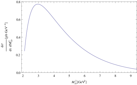
Figure 5: The $M_{\gamma\gamma}^{2}$ dependence of the unpolarized differential cross section $\frac{d\sigma}{dM_{\gamma\gamma}^{2}dt}$ on a proton(left panel) and on a neutron(right panel) at $t=t_{min}$ and $S_{\gamma N}=20$ GeV² (full curves), $S_{\gamma N}=100$ GeV² (dashed curve) and $S_{\gamma N}=10^{6}$ GeV² (dash-dotted curve, multiplied by $10^{5}$). The range of integration with respect to $u^{\prime}$ is explained in the text.

Integration over $M^{2}_{\gamma\gamma}$ over the range $M_{\gamma\gamma}^{2}>2$ GeV² leads to the $u^{\prime}$ dependence:

$$\left.\int_{2}dM_{\gamma\gamma}^{2}~{}\frac{d\sigma}{dM_{\gamma\gamma}^{2}dt(-du^{\prime})}\right|_{t=t_{min}(M_{\gamma\gamma}^{2})}=\left.\frac{d\sigma}{dtd(-u^{\prime})}\right|_{t=t_{min}}$$ (34)

We show this differential cross section on Fig. 6 for a proton and neutron target.

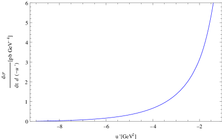
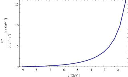
Figure 6: The $u^{\prime}$ dependence of the unpolarized differential cross section $\frac{d\sigma}{dtdu^{\prime}}$ on a proton (left panel) and on a neutron (right panel) at $t=t_{min}$ and $S_{\gamma N}=20GeV^{2}$, integrated over $M_{\gamma\gamma}^{2}$ as explained in the text.

The conclusion of these cross-section estimates is straightforward. This reaction can be studied at intense photon beam facilities in JLab. The rates are not very large but of comparable order of magnitude as those for the timelike Compton scattering reaction, the feasibility of which has been demonstrated Boer . Since there are no contribution from gluons and sea-quarks, one does not get larger cross-sections at higher energies. Contrarily to timelike Compton scattering PSWUPC , it thus does not seem attractive to look for this reaction in ultra peripheral reactions at hadron colliders.

V Polarization asymmetries

V.1 Circular initial photon polarization

Defining as usual the two circular polarization states of the incoming photon as

$$\epsilon_{\bot}^{\mu}(q,+)=-\frac{1}{\sqrt{2}}\left(\epsilon_{\bot}^{\mu}(q,x)+i\epsilon_{\bot}^{\mu}(q,y)\right)\,,\;\;\;\;\;\;\epsilon_{\bot}^{\mu}(q,-)=\frac{1}{\sqrt{2}}\left(\epsilon_{\bot}^{\mu}(q,x)-i\epsilon_{\bot}^{\mu}(q,y)\right)\,,$$ (35)

the electromagnetic tensor entering the polarized cross section difference reads

$$\epsilon_{\bot}^{\mu}(q,+)\epsilon_{\bot}^{\nu*}(q,+)-\epsilon_{\bot}^{\mu}(q,-)\epsilon_{\bot}^{\nu*}(q,-)=i\left(\epsilon_{\bot}^{\mu}(q,y)\epsilon_{\bot}^{\nu}(q,x)-\epsilon_{\bot}^{\mu}(q,x)\epsilon_{\bot}^{\nu}(q,y)\right)=-i\frac{2}{s}\epsilon^{\mu\nu pn}\,,$$ (36)

which leads to a cross-section difference

$${\cal T}_{+}{\cal T}^{*}_{+}-{\cal T}_{-}{\cal T}^{*}_{-}\sim|\Delta_{t}||p_{t}|\sin(\phi)\,.$$ (37)

The circular polarization asymmetry is thus of $O(\frac{\Delta_{T}}{Q})$. It is thus inconsistent to calculate it from our formulae since twist 3 contributions that we did not consider, in particular those mandated by electromagnetic gauge invariance twist3 are of the same order.

Figure 7: The azimuthal dependence of the differential cross section $\frac{d\sigma}{dM_{\gamma\gamma}^{2}dtdu^{\prime}d\phi}$ at $t=t_{min}$ and $S_{\gamma N}=20$ GeV². $(M_{\gamma\gamma}^{2},u^{\prime})=(3,-2)$ GeV² (solid line), $(M_{\gamma\gamma}^{2},u^{\prime})=(4,-1)$ GeV² (dotted line) and $(M_{\gamma\gamma}^{2},u^{\prime})=(4,-2)$ GeV² (dashed line). $\phi$ is the angle between the initial photon polarization and one of the final photon momentum in the transverse plane.

V.2 Linear initial photon polarization

Linearly polarized real photons open the way to large asymmetries, as they do for dilepton photoproduction Goritschnig:2014eba . Let us consider the case where the initial photon is polarized along the $x$ axis, : $\epsilon(q)=(0,1,0,0)$ and define the azimuthal angle $\phi$ through

$$p_{T}^{\mu}=(0,~{}p_{T}~{}cos\phi,~{}p_{T}~{}sin\phi,0).$$

The cross section exhibits then an azimuthal dependence, and one should calculate

$$\frac{d\sigma_{l}}{dM^{2}_{\gamma\gamma}dtd(-u^{\prime})d\phi}=\frac{1}{2}\frac{1}{(2\pi)^{4}32S^{2}_{\gamma N}M^{2}_{\gamma\gamma}}\sum_{\lambda_{1}\lambda_{2},s_{1},s_{2}}\frac{|\mathcal{T}|^{2}}{2}.$$ (38)

This is shown on Fig. 7 for different values of $(M_{\gamma\gamma}^{2},u^{\prime})$ at $t=t_{min}$ and $S_{\gamma N}=20$ GeV². As straightforwardly anticipated, the cross section shows a modulation of the form $A+B~{}cos2\phi$. It turns out that $B$ is negative leading to a minimum at $\phi=0$ and a maximum at $\phi=\pi/2$. In all cases, the linear polarization effects are huge.

VI Conclusion

Our calculation of the leading order leading twist amplitude of reaction (1) has demonstrated that the photoproduction of a large invariant mass diphoton is an interesting process to analyze in the collinear factorization framework. The amplitude has very specific properties which should be very useful for future GPDs extractions programs e.g. PARTONS .

The $O(\alpha_{s})$ corrections to the amplitude need to be calculated.They are particularly interesting since they open the way to a perturbative proof of factorization. Moreover, let us recall the reader of the importance of the timelike vs spacelike nature of the probe with respect to the size of the NLO corrections MPSW ; since the hard scales at work in our process are both the timelike one $M^{2}_{\gamma\gamma}$ and the spacelike one $u^{\prime}$, we are facing an intermediate case between timelike Compton scattering and spacelike DVCS.

In this paper, we only addressed the leading twist amplitude. There are more than one source of $O(\frac{1}{Q})$ corrections to the amplitude. The inclusion of finite hadron mass and finite $t$ effects has been discussed in great detail in BraunManashov for the DVCS case and we believe that they can be included in the same way for the reaction studied here. There is an interesting other piece of higher twist contribution which we may solve right away. This is the part related to the twist 2 distribution amplitude of the final photons. Indeed, this contribution may be read off the formulae written in Ref. Boussarie:2016qop where the process $\gamma N\to\gamma\rho(\varepsilon_{T})N^{\prime}$ was calculated. Indeed the real photon DA photonDA has the same chiral-odd structure as the transversely polarized $\rho$ meson, and thus its contribution to the scattering amplitude may be deduced from the $\gamma\rho^{0}_{T}$ meson case, by replacing $\frac{f_{\rho}}{\sqrt{2}}$ in the normalization of the meson DA by the constant $e_{q}\chi<\bar{q}q>$ including the magnetic susceptibility $\chi$ of the QCD vacuum. Theoretical estimates photonDA of $\chi<\bar{q}q>$ are around $50$ MeV. Using numerical estimates of Ref. Boussarie:2016qop , this leads to a smaller than $10\%$ correction to the cross section already at $M^{2}_{\gamma\gamma}=3$ GeV². Including the contributions of higher twist GPDs is a tougher job which will need long further studies Anikin:2009hk ; indeed factorization may even break down.

We only addressed the case of a real photon beam. The analysis of the corresponding reaction with quasi real photons obtained from a lepton beam goes along the same lines but needs to be complemented by the analysis of the Bethe Heitler processes where one or two photons are emitted from the lepton line. The relative magnitude of this background to the QCD process is likely to depend much on the energy and on the azimuth of the produced photons, as it is the case in the known example of DVCS. We can anticipate that the contribution of the double Bethe Heitler process $e^{-}\to e^{-}\gamma^{*}(t)~{}\gamma~{}\gamma$ to the reaction $e^{-}N\to e^{-}\gamma~{}\gamma~{}N^{\prime}$ will dominate at small $t$. This should lead to interesting interference effects with the amplitude that we studied here, as in the well-know case of DVCS. We shall study this case in details in a future work.

Acknowledgements.

We acknowledge useful conversations with Renaud Boussarie, Michel Guidal, Hervé Moutarde and Samuel Wallon. This work is partly supported by Grant No. 2015/17/B/ST2/01838 from the National Science Center in Poland, by the Polish-French collaboration agreements Polonium and COPIN-IN2P3, and by the French Grant ANR PARTONS (Grant No. ANR-12-MONU-0008-01).

References

(1)
D. Müller et al.,
Fortsch. Phys. 42, 101 (1994);
X. Ji,
Phys. Rev. Lett. 78, 610 (1997);
A. V. Radyushkin,
Phys. Rev. D 56, 5524 (1997);
M. Diehl, T. Gousset, B. Pire, and J. P. Ralston,
Phys. Lett. B 411, 193 (1997);
J. C. Collins and A. Freund,
Phys. Rev. D 59, 074009 (1999);
E. R. Berger, M. Diehl, and B. Pire,
Eur. Phys. J. C 23, 675 (2002).
(2)
M. Diehl,
Phys. Rept. 388 (2003) 41;
A. V. Belitsky and A. V. Radyushkin,
Phys. Rept. 418, 1 (2005);
S. Boffi and B. Pasquini,
Riv. Nuovo Cim. Soc. Ital. Fis. 30, 387 (2007).
(3)
D. Yu. Ivanov, B. Pire, L. Szymanowski ,and O. V. Teryaev,
Phys. Lett. B 550, 65 (2002);
R. Enberg, B. Pire, and L. Szymanowski,
Eur. Phys. J. C 47, 87 (2006);
S. Kumano, M. Strikman and K. Sudoh,
Phys. Rev. D 80, 074003 (2009).
(4)
M. El Beiyad, B. Pire, M. Segond, L. Szymanowski and S. Wallon,
Phys. Lett. B 688, 154 (2010).
(5)
S. V. Goloskokov and P. Kroll,
Eur. Phys. J. C 53 , 367 (2008) ;
P. Kroll, H. Moutarde and F. Sabatié,
Eur. Phys. J. C 73 , 2278(2013) .
(6)
M. Vanderhaeghen, P. A. M. Guichon and M. Guidal,
Phys. Rev. D 60, 094017 (1999).
(7)
M. Burkardt,
Phys. Rev. D 62, 071503 (2000)
Erratum: [Phys. Rev. D 66 , 119903 (2002) ];
M. Diehl,
Eur. Phys. J. C 25, 223 (2002);
Erratum: [Eur. Phys. J. C 31, 277 (2003) ];
J. P. Ralston and B. Pire,
Phys. Rev. D 66, 111501(2002).
(8)
B. Pire, L. Szymanowski and J. Wagner,
Phys. Rev. D 79, 014010 (2009).
(9)
J. L. Abelleira Fernandez et al. [LHeC Study Group],
J. Phys. G 39, 075001 (2012).
(10)
M. Boer, M. Guidal and M. Vanderhaeghen,
Eur. Phys. J. A 51, 103 (2015).
(11)
I. V. Anikin, B. Pire and O. V. Teryaev,
Phys. Rev. D 62, 071501 (2000) ;
A. V. Belitsky and D. Mueller,
Nucl. Phys. B589, 611 (2000).
(12)
A. T. Goritschnig, B. Pire and J. Wagner,
Phys. Rev. D 89, 094031 (2014).
(13)
B. Berthou et al.,
arXiv:1512.06174.
(14)
B. Pire, L. Szymanowski and J. Wagner,
Phys. Rev. D 83 , 034009 (2011),
Few Body Systems 53, 125 (2012);
D. Mueller, B. Pire, L. Szymanowski and J. Wagner,
Phys. Rev. D 86, 031502 (2012);
H. Moutarde, B. Pire, F. Sabatie, L. Szymanowski and J. Wagner,
Phys. Rev. D 87 , 054029 (2013).
(15)
V. M. Braun and A. N. Manashov,
Phys. Rev. Lett. 107, 202001 (2011);
V. M. Braun, A. N. Manashov and B. Pirnay,
Phys. Rev. Lett. 109, 242001 (2012);
V. M. Braun, A. N. Manashov, D. M ller and B. M. Pirnay,
Phys. Rev. D 89, 074022 (2014).
(16)
R. Boussarie, B. Pire, L. Szymanowski and S. Wallon,
JHEP 1702, 054 (2017).
(17)
P. Ball, V. M. Braun and N. Kivel,
Nucl. Phys. B649, 263 (2003);
V. M. Braun, S. Gottwald, D. Y. Ivanov, A. Schafer and L. Szymanowski,
Phys. Rev. Lett. 89, 172001 (2002);
B. Pire and L. Szymanowski,
Phys. Rev. Lett. 103, 072002 (2009).
(18)
I. V. Anikin, D. Y. Ivanov, B. Pire, L. Szymanowski and S. Wallon,
Phys. Lett. B 682, 413 (2010);
I. V. Anikin, D. Y. Ivanov, B. Pire, L. Szymanowski and S. Wallon,
Nucl. Phys. B828, 1 (2010).