Practical Statistics

Abstract

Accelerators and detectors are expensive, both in terms of money and human effort. It is thus important to invest effort in performing a good statistical analysis of the data, in order to extract the best information from it. This series of five lectures deals with practical aspects of statistical issues that arise in typical High Energy Physics analyses.

Keywords
Statistics; lectures ; data analysis method; statistical analysis; frequentist; Bayesian.

1 Outline

This series of five lectures deals with practical aspects of statistical issues that arise in typical High Energy Physics analyses. The topics are:

• Introduction. This is largely a reminder of topics which you should have encountered as undergraduates. Some of them are looked at in novel ways, and will hopefully provide new insights.

• Least Squares and Likelihoods. We deal with two different methods for parameter determination. Least Squares is also useful for Goodness of Fit testing, while likelihood ratios play a crucial role in choosing between two hypotheses.

• Bayes and Frequentism. These are two fundamental and very different approaches to statistical searches. They disagree even in their views on ‘What is probability?’

• Searches for New Physics. Many statistical issues arise in searches for New Physics. These may result in discovery claims, or alternatively in exclusion of theoretical models in some region of their parameter space (e.g. mass ranges).

• Learning to love the covariance matrix. This is relevant for dealing with the possible correlations between uncertainties on two or more quantities. The covariance matrix takes care of all these correlations, so that you do not have to worry about each situation separately. This was an unscheduled lecture which was included at the request of several students.

Lectures 3 to 5 are not included in these proceedings but can be found elsewhere [1, 2, 3].

The material in these lectures follows loosely that in my book [4], together with some significant updates (see ref. [5]).

2 Introduction to Lecture 1

The first lecture, covered in Sections 2 to 11, is a recapitulation of material that should already be familiar, but hopefully with some new emphases. We start with a a discusssion of ‘What is Statistics?’ and a comparison of ‘Statistics’ and ’Probability’. Next the importance of calculating uncertainties is emphasised, as well as the difference between random and systematic uncertainties.

The following sections are about combinations. The first is about how to combine different individual contributions to a particlar experimental result; the second is the combination of two or more separate experimental determinaions of the same physical quantity.

The final topics are the Binomial, Poisson and Gaussian probability distributions. Undertanding of these is important for many statistical analyses.

3 What is Statistics?

Statistics is used to provide quantitative results that give summaries of available data. In High Energy Physics, there are several different types of statistical activities that are used:

• Parameter Determination:
  We analyse the data in order to extract the best value(s) of one or more parameters in a model. This could be, for example, the gradient and intercept of a straight line fit to the data; or the mass of the Higgs boson, as deduced using its decay products. In all cases, as well as obtaining the best values of the parameter(s), their uncertainties and possible correlations must be specified.

• Goodness of Fit:
  We are comparing a single theory with the data, in order to see if they are compatible. If the theory contains free parameters, their best values need to be used to check the Goodness of Fit. If the quality of the fit is unsatisfactory, the best values of the parameters are probably meaningless.

• Hypothesis Testing:
  Here we are comparing the data with two different theories, to see which provides a better description. For example, we may be very interested in knowing whether a model involving the production of a supersymmetric particle is better than one without it.

• Decision Making:
  As the result of the information we have available, we want to decide what further action to take. For example, we may have some evidence that our data shows hints of an exciting discovery, and need to decide whether we should collect more data. This was the situation faced by the CERN management in 2000, when there were perhaps hints of a Higgs boson in data collected at the LEP Collider.

  Such decisions usually require a ‘cost function’ for the various possible outcomes, as well as assessments of their relative probabilities. In the example just quoted, numerical values were needed for the cost of missing an important discovery if the experiment was not continued; and on the other hand of running the LEP Collider for another year and for delaying the start of building the Large Hadron Collider.

  Decision Making is not considered further in these lectures.

4 Probability and Statistics

Probability theory involves starting with a model, and using it to make predictions about possible outcomes of an experiment where randomness plays a role; it involves precise mathematics, and in general there is only one correct solution about the probabilities of the different outcomes. Statistics involves the opposite procedure of using the observed data in order to make statements about the relevant theory or model. This is usually not a precise process and there may be different approaches which yield different answers, none of which being necessarily invalid.

The example of throwing dice (see Table 1) illustrates the relationship of Probability Theory and Statistics for some of the statistical procedures.

Table 1: Probability and Statistics: Throwing dice

Probability	Statistics	Procedure
Given p(5) =1/6,	Given 20 5s in 100 trials,
what is prob(20 5s in 100 trials)?	what is p(5)?
	and its uncertainty?	Parameter Determination
If unbiassed,	Given 60 evens in 100 trials,
what is prob(n evens in 100 trials)?	is it unbiassed?	Goodness of Fit
	Or is prob(evens) = 2/3?	Hypothesis Testing
THEORY $\rightarrow$ DATA	DATA $\rightarrow$ THEORY

5 Why uncertainties?

Without an estimate of the uncertainty of a parameter, its central value is essentially useless. This is illustrated by Table 2. The three lines of the Table refer to different possible results; all have the same central value of the ratio of the experimental result divided by the theoretical prediction, but each has a different uncertainty on this ratio. The conclusions about whether the data supports the theory are very different, depending on the magnitude of the uncertainty, even though the central values are the same for each of the three situations. It is thus crucial to estimate uncertainties accurately, and also correlations when measuring two or more parameters.

Table 2: Experiment testing General Relativity.

Experiment/Theory	Uncertainty	Conclusion
0.970	$\pm$ 0.05	Consistent with 1.0
0.970	$\pm$ 0.006	Inconsistent with 1.0
0.970	$\pm$ 0.7	Do a better experiment

6 Random and systematic uncertainties

Random or statistical uncertainties result from the limited accuracy of measurements, or from the fluctuations that arise in counting experiments where the Poisson distribution is relevant (see Section 10). If the experiment is repeated, the results will vary somewhat, and the spread of the answers provides (not necessarily the best) estimate of the statistical uncertainty.

Systematic uncertainties can also arise in the measuring process. The quantities we measure may be shifted from the true values. For example, our measuring device may be miscalibrated, or the number of events we count may be not only from the desired signal, but also from various background sources. Such effects would bias our result, and we should correct for them, for example by performing some calibration measurement. The systematic uncertainty arises from the remaining uncertainty in our corrections. Systematics can cause a similar shift in a repeated series of experiments, and so, in contrast to statistical uncertainties, they may not be detectable by looking for a spread in the results.

For example consider a pendulum experiment designed to measure the acceleration due to gravity $g$ at sea level in a given location:

$$g=4\pi^{2}L/\tau^{2}$$ (1)

where $L$ is the length of the pendulum, $\tau=T/N$ is its period, and $T$ is the time for $N$ oscillations. The uncertainties we have mentioned so far are the statistical ones on $L$ and $T$. There may also be systematic uncertainties on these variables.

Unfortunately there are further possible systematics not associated with the measured quantities, and which thus require more careful consideration. For example, the derivation of eqn. (1) assumes that:

• our pendulum is simple i.e. the string is massless, and has a massive bob of infinitesimal size;

• the support of the pendulum is rigid;

• the oscillations are of very small amplitude (so that $\sin\theta\approx\theta)$; and

• they are undamped.

None of these will be exact in practice, and so corrections must be estimated for them. The uncertainties in these corrections are systematics.

Furthermore, there may be theoretical uncertainties. For example, we may want the value of $g$ at sea level, but the measurements were performed on top of a mountain. We thus need to apply a correction, which depends on our elevation and on the local geology. There might be two or more different theoretical correction factors, and again this will contribute a systematic uncertainty.

6.1 Presenting the results

A common way of presenting the result of a measurement $y$ is as $y\pm\sigma_{stat}\pm\sigma_{syst}$, where the statistical and systematic uncertainties are shown separately. Alternatively, it may be presented as $y\pm\sigma$, where the total uncertainty is usually given by $\sigma^{2}=\sigma_{stat}^{2}+\sigma_{syst}^{2}$.

The other extreme is to give a list of all the individual systematics separately (usually in a Table, rather than in the Abstract or Conclusions). The motivations for this are that:

• systematics are sometimes caused by uncertainties in other people’s measurements of some relevant quantity. If subsequently this measurement is updated, it will be possible to reduce the systematic uncertainty appropriately; and

• our measurement may be combined with others to produce a ‘World average’, or it may be used together with another result to calculate something else. In both these cases, correlations between the different experimental measurements are needed, and so the individual sources are required.

For example, it may be interesting to compare the sea-level values of $g$ at the same location several years apart. In that case, although there might be significant uncertainties from the correction of the measurements to sea-level, they are a fully correlated, and so will cancel in their difference

7 Combining uncertainties

In this section, we consider how to estimate the uncertainty $\sigma_{z}$ in a quantity of interest $z$, which is defined in terms of measured quantities $x,y,....$ by a known function $z(x,y,.....)$. The uncertainties on the measured quantities are known and assumed to be uncorrelated. The recipe for $\sigma_{z}$ depends on the functional form of $z$.

7.1 Linear forms

As a very simple example, consider

$$z=x-y$$ (2)

From this, we obtain

$$\delta z=\delta x-\delta y$$ (3)

where $\delta z$ is the change in $z$ that would be produced by specific changes in $x$ and $y$. But eqn. 3 refers to specific offsets, rather than the uncertainties $\sigma_{z}$, etc, which are the RMS values of the offsets i.e. $\overline{\delta z^{2}}$, etc. Thus we need to square eqn. 3, which yields

$$\delta z^{2}=\delta x^{2}+\delta y^{2}-2\delta x\delta y,$$ (4)

and to average over a whole series of measurements. We then obtain the correct formula for combining the uncertainties:

$$\sigma_{z}^{2}=\sigma_{x}^{2}+\sigma_{y}^{2},$$ (5)

provided we ignore the last term in eqn 4. The justification for this is that the average value of $\delta x\delta y$ is zero, provided the uncertainties on $x$ and on $y$ are uncorrelated.

For the general linear form

$$z=k_{1}x+k_{2}y+.......$$ (6)

where $k_{1},k_{2},....$ are constants, the uncertainty on $z$ is given by

$$\sigma_{z}=k_{1}\sigma_{x}\ \&\ k_{2}\sigma_{y}\ \&\ .......\ ,$$ (7)

where the symbol $\&$ is used to mean “combine using Pythagoras’ Theorem". For the special case of $z=x-y$, as is expected this gives the result of eqn. 5 for $\sigma_{z}$.

For this case of $z$ being a linear function of the measurements, it is the absolute uncertainties that are relevant for determining $\sigma_{z}$. It is important not to use fractional uncertainties. Thus if you want to determine your height by making independent measurements of the distances of the top of your head and the bottom of your feet from the centre of the earth, each with an accuracy of 1 part in 1000, you will not determine your height to anything like 1 part in 1000.

7.2 Products and quotients

The general form here is

$$z=x^{\alpha}y^{\beta}......,$$ (8)

where the powers $\alpha,\beta,$ etc. are constants. This includes forms such as $x^{2},\ y^{3}/x,\sqrt{x}/y$, etc. The formula for combining the uncertainties is

$$\sigma_{z}/z=\alpha\sigma_{x}/x\ \&\ \beta\sigma_{y}/y\ \&\ ....$$ (9)

That is, the fractional uncertainty on $z$ is derived from the fractional uncertainties on the measurements.

Because this result was derived by taking the first term of a Taylor expansion for $\delta z$, it will be a good approximation only for small uncertainties. If the uncertainties are large, more sophisticated approaches are required for determining the uncertainty in $z$. This also applies to the next section, but is irrelevant for the linear cases discussed above, as all terms in the Taylor series beyond those involving first derivatives are zero.

7.3 All other functions

Finally we deal with any functional form $z=z(x_{1},x_{2},x_{3},.....)$. Our prescription of writing down the first term in the Taylor series expansion for $\delta z$, squaring and averaging gives

$$\sigma_{z}=\frac{\partial z}{\partial x_{1}}\sigma_{1}\ \&\ \frac{\partial z}{\partial x_{2}}\sigma_{2}\ \&\ ....$$ (10)

where the $\sigma_{i}$ are the uncertainties on $x_{i}$, again assumed uncorrelated.

A slightly easier method to apply is to use a numerical approach for calculating the partial derivatives. We evaluate

$$\begin{split}z_{0}&=z(x_{1},x_{2},x_{3},....)\\ z_{1}&=z(x_{1}+\sigma_{1},x_{2},x_{3},....)\\ z_{2}&=z(x_{1},x_{2}+\sigma_{2},x_{3},....)\\ z_{3}&=z(x_{1},x_{2},x_{3}+\sigma_{3},....)\\ &\ \ \ \ \ \ \ \ etc.\end{split}$$ (11)

and then

$$\sigma_{z}^{2}=\Sigma(z_{i}-z_{0})^{2}$$ (12)

8 Combining experiments

Sometimes different experiments will measure the same physical quantity. It is then reasonable to ask what is our best information available when these experiments are combined. It is a general rule that it is better to use the DATA for the experiments and then perform a combined analysis, rather than simply combine the RESULTS. However, combining the results is a simpler procedure, and access to the original data is not always possible.

For a series of unbiassed, uncorrelated measurements $x_{i}$ of the same physical quantity, the combined value $\hat{x}\pm\hat{\sigma}$ is given by weighting each measurement by $w_{i}$, which is proportional to the inverse of the square of its uncertainty i.e.

$$\hat{x}=\Sigma w_{i}x_{i},\ \ \ \ w_{i}=(1/\sigma_{i}^{2})/\Sigma(1/\sigma_{j}^{2})$$ (13)

with the uncertainty $\hat{\sigma}$ on the combined value being given by

$$1/\hat{\sigma}^{2}=\Sigma 1/\sigma_{i}^{2}$$ (14)

This ensures that the uncertainty on the combination is at least as small as the smallest uncertainty of the individual measurements. It should be remembered that the combined uncertainty takes no account of whether or not the individual measurements are consistent with each other.

In an informal sense, $1/\sigma_{i}^{2}$ is the information content of a measurement. Then each $x_{i}$ is weighted proportionally to its information content. Also the equation for $\hat{\sigma^{2}}$ says that the information content of the combination is the sum of the information contents of the individual measurements.

An example demonstrates that care is needed in applying the formulae. Consider counting the number of high energy cosmic rays being recorded by a large counter system for two consecutive one-week periods, with the number of counts being $100\pm 10$ and $1\pm 1$ . (See section 10 for the choice of uncertainties). Unthinking application of the formulae for the combined result give the ridiculous $2\pm 1$. What has gone wrong?

The answer is that we are supposed to use the true accuracies of the individual measurements to assign the weights. Here we have used the estimated accuracies. Because the estimated uncertainty depends on the estimated rate, a downward fluctuation in the measurement results in an underestimated uncertainty, an overestimated weight, and a downward bias in the combination. In our example, the combination should assume that the true rate was the same in the two measurements which used the same detector and which lasted the same time as each other, and hence their true accuracies are (unknown but) equal. So the two measurements should each be given a weight of 0.5, which yields the sensible combined result of $50.5\pm 5$ counts.

8.1 BLUE

A method of combining correlated results is the ‘Best Linear Unbiassed Estimate’ (BLUE). We look for the best linear unbiassed combination

$$x_{BLUE}=\Sigma w_{i}x_{i},$$ (15)

where the weights are chosen to give the smallest uncertainty $\sigma_{BLUE}$ on $x_{BLUE}$. Also for the combination to be unbiassed, the weights must add up to unity. They are thus determined by minimising $\Sigma\Sigma w_{i}w_{j}E^{-1}_{ij}$, subject to the constraint $\Sigma w_{i}=1$; here $E$ is the covariance matrix for the correlated measurements.

The $BLUE$ procedure just described is equivalent to the $\chi^{2}$ approach for checking whether a correlated set of measurements are consistent with a common value. The advantage of $BLUE$ is that it provides the weights for each measurement in the combination. It thus enables us to calculate the contribution of various sources of uncertainty in the individual measurements to the uncertainty on the combined result.

8.2 Why weighted averaging can be better than simple averaging

Consider a remote island whose inhabitants are very conservative, and no-one leaves or arrives except for some anthropologists who wish to determine the number of married people there. Because the islanders are very traditional, it is necessary to send two teams of anthropologists, one consisting of males to interview the men, and the other of females for the women. There are too many islanders to interview them all, so each team interviews a sample and then extrapolates. The first team estimates the number of married men as $10,000\pm 300$. The second, who unfortunately have less funding and so can interview only a smaller sample, have a larger statistical uncertainty; they estimate $9,000\pm 900$ married women. Then how many married people are there on the island?

The simple approach is to add the numbers of married men and women, to give $19,000\pm 950$ married people. But if we use some theoretical input, maybe we can improve the accuracy of our estimate. So if we assume that the islanders are monogamous, the numbers of married men and women should be equal, as they are both estimates of the number of married couples. The weighted average is $9,900\pm 285$ married couples and hence $19,800\pm 570$ married people.

The contrast in these results is not so much the difference in the estimates, but that incorporating the assumption of monogamy and hence using the weighted average gives a smaller uncertainty on the answer. Of course, if our assumption is incorrect, this answer will be biassed.

A Particle Physics example incorporating the same idea of theoretical input reducing the uncertainty of a measurement can be found in the ‘Kinematic Fitting’ section of Lecture 2.

9 Binomial distribution

This and the next sections on the Poisson and Gaussian distributions are probability theory, in that they make statements about the probabilities of different outcomes, assuming that the thoretical distribution is known. However, the results are important for Statistics, where we use data in order to make statements about theory.

The binomial distribution applies when we have a set of $N$ independent trials, in each of which a ‘success’ occurs with probability $p$. Then the probability $P(s;N,p)$ of $s$ successes in the $N$ trials is obviously

$$P(s;N,p)=\frac{N!}{s!\ (N-s)!}\ p^{s}\ (1-p)^{N-s}.$$ (16)

An example of a Binomial distribution would be the number of times we have a 6 in 20 throws of a die; or the distribution of the number of successfully reconstructed tracks in a sample of 100, when the probability for reconstructing each of them is 0.98

The expected number of successes $<\!\!s\!\!>$ is $\Sigma s\times P(s;N,p)$, which after some algebra turns out to be (not surprisingly) $Np$. The variance $\sigma_{s}^{2}$ of the distribution in $s$ is obviously given by $Np(1-p)$. Note that, while for the Poisson distribution the mean and variance are equal, this is not so in general for the Binomial - it is approximately so at small $p$.

As an example several Binomial distributions with fixed number of trials $N$ but varying probabilities of success $p$ are shown in Fig. 1.

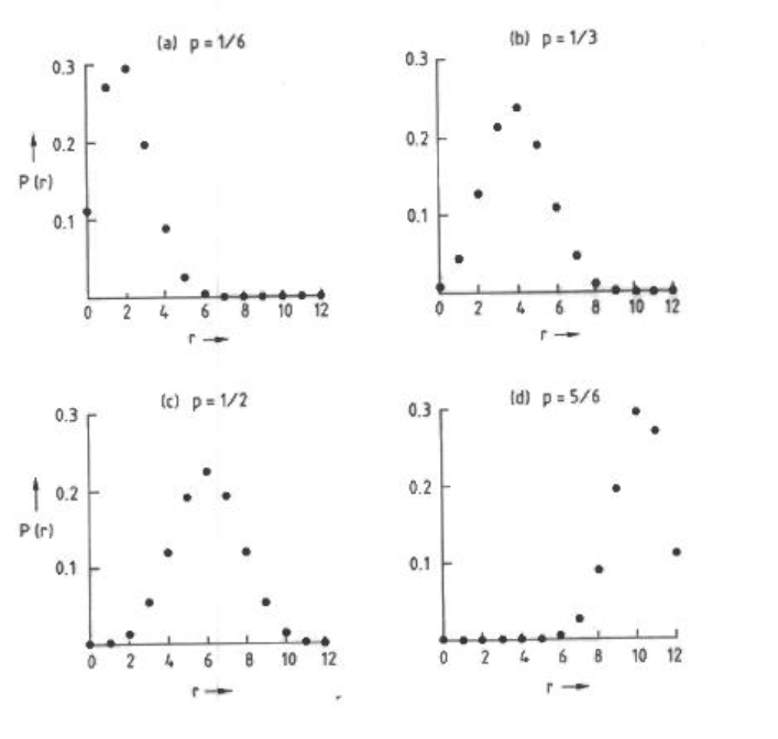
Figure 1: The probabilities $P(r)$ according to the binomial distribution, for $r$ successes out of 12 independent trials, when the probability $p$ of success in an individual trial is as specified. As the expected number of successes is $12p$, the peak of the distribution moves to the right as $p$ increases. The variance of the distribution is $12p(1-p)$ and hence is largest for $p=1/2$. Since the chance of success when $p=1/6$ is the same as that for failure when $p=5/6$, diagrams (a) and (d) are mirror images of each other. Similarly for $p=1/2$ (see (c)) the distribution is symmetric about $r=6$ successes.

10 Poisson distribution

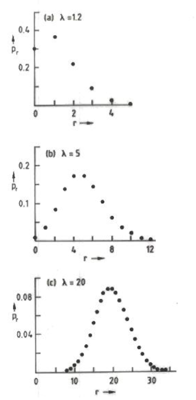
Figure 2: Poisson distributions for various values of the Poisson parameter $\lambda$: (a) $\lambda=1.2$ (b) $\lambda=5.0$ (c) $\lambda=20.0$. $P_{r}$ is the probability for observing $r$ events. For each $\lambda$, the mean value of $r$ is $\lambda$ and the RMS width is $\sqrt{\lambda}$. As $\lambda$ increases above about 10, the distribution becomes more like a Gaussian.

The Poisson distribution (see Fig. 2) applies to situations where we are counting a series of observations which are occuring randomly and independently during a fixed time interval $t$, where the underlying rate $r$ is constant. The observed number $n$ will fluctuate when the experiment is repeated, and can in principle take any integer value from zero to infinity. The Poisson probabilty of observing $n$ decays is given by

$$P_{n}=e^{-rt}(rt)^{n}/n!$$ (17)

It applies to the number of decays observed from a large number $N$ of radioactive nuclei, when the observation time $t$ is small compared to the lifetime $\tau$. It will not apply if $t$ is much larger than $\tau$, or if the detection system has a dead time, so that after observing a decay the detector cannot observe another decay for a period $T_{dead}$.

Another example is the number of counts in any specific bin of a histogram when the data is accumulated over a fixed time.

The average number of observations is given by

$$<n>=\Sigma nP_{n}=rt$$ (18)

If we write the expected number as $\mu$, the Poisson probability becomes

$$P_{n}=e^{-\mu}\mu^{n}/n!$$ (19)

It is also relatively easy to show that the variance

$$\sigma^{2}=\Sigma(n-\mu)^{2}P_{n}=\mu$$ (20)

This leads to the well-known $n\pm\sqrt{n}$ approximation for the value of the Poisson parameter when we have $n$ counts. This approximation is, however, particularly bad when there are zero observed events; then $0\pm 0$ incorrectly suggests that the Poisson parameter can be only zero.

Poisson probabilities can be regarded as the limit of Binomial ones as the number of trials $N$ tends to infinity and the Binomial probability of success $p$ tends to zero, but the product $Np$ remains constant at $\mu$.

When the Poisson mean becomes large, the distribution of observed counts approximates to a Gaussian (although the Gaussian is a continuous distribution extending down to $-\infty$, while a Poisson observable can only take on non-negative integral values). This approximation is useful for the $\chi^{2}$ method for parameter estimation and goodness of fit (see Lecture 2).

10.1 Relation of Poisson and Binomial Distributions

An interesting example of the relationship between the Poisson and Binomial distributions is exhibited by the following example.

Imagine that the number of people attending a series of lectures is Poisson distributed with a constant mean $\nu$, and that the fraction of them who are male is $p$. Then the overall probability $P$ of having N people of whom $M$ are male and $F=N-M$ are female is given by the product of the Poisson probability $P_{pois}$ for $N$ and the binomial probability $P_{bin}$ for $M$ of the $N$ people being male. i.e.

$$P=P_{pois}P_{bin}=\frac{e^{-\nu}\nu^{N}}{N!}\times\frac{N!}{M!F!}p^{M}(1-p)^{F}$$ (21)

This can be rearranged as

$$P=\frac{e^{-\nu p}(\nu p)^{M}}{M!}\times\frac{e^{-\nu(1-p)}(\nu(1-p))^{F}}{F!}$$ (22)

This is the product of two Poissons, one with Poisson parameter $\nu p$, the expected number of males, and the other with parameter $\nu(1-p)$, the expected number of females. Thus with a Poisson-varying total number of observations, divided into two categories (here male and female), we can regard this as Poissonian in the total number and Binomial in the separate categories, or as two independent Poissons, one for each category. Other situations to which this applies could be radioactive nuclei, with decays detected in the forward or backward hemispheres; cosmic ray showers, initiated by protons or by heavier nuclei; patients arriving at a hospital emergency centre, who survive or who die; etc.

10.2 For your thought

The first few Poisson probabilities $P(n;\mu)$ are

$$\begin{split}P(0)=e^{-\mu},\ \ \ \ \ P(1)=\mu e^{-\mu},\ \ \ \ \ P(2)=(\mu^{2}/2!)\ e^{-\mu},\ \ \ \ \ etc.\end{split}$$ (23)

Thus for small $\mu$, $P(1)$ and $P(2)$ are approximately $\mu$ and $\mu^{2}/2$ respectively. But if the probability of one rare event happening is $\mu$, why is the probability for 2 independent rare events not equal to $\mu^{2}$?

11 Gaussian distribution

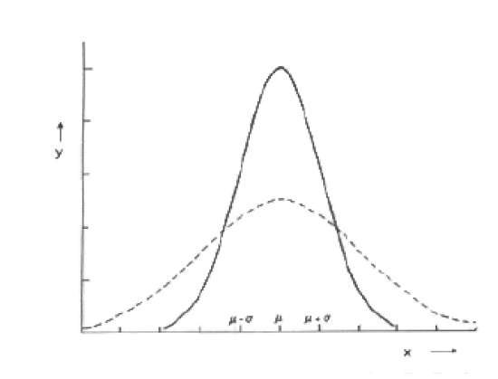
Figure 3: Gaussian distributions. Both are centred at $x=\mu$, but the dashed curve is twice as wide as the solid one. Because they have the same normalisation the maximum of the solid curve curve is twice as high as that of the dashed one. The scale on the horizontal axis refers to the solid curve.

The Gaussian or normal distribution (shown in Fig. 3) is of widespread usage in data analysis. Under suitable conditions, in a repeated series of measurements $x$ with accuracy $\sigma$ when the true value of the quantity is $\mu$, the distribution of $x$ is given by a Gaussian. A mathematical motivation is given by the Central Limit Theorem, which states that the sum of a large number of variables with (almost) any distributions is approximately Gaussian.

For the Gaussian, the probability density $y(x)$ of an observation $x$ is given by

$$y(x)=\frac{1}{\sqrt{2\pi}\sigma}e^{-\frac{(x-\mu)^{2}}{2\sigma^{2}}}$$ (24)

where the parameters $\mu$ and $\sigma$ are respectively the centre and width of the distribution. The factor $1/(\sqrt{2\pi}\sigma)$ is required to normalise the area under the curve, so that $y(x)$ can be directly interpreted as a probability density.

There are several properties of $\sigma$:

• The mean value of $x$ is $\mu$, and the standard deviation of its distribution is $\sigma$. Since the usual symbol for standard deviation is $\sigma$, this leads to the formula $\sigma=\sigma$ (which is not so trivial as it seems, since the two $\sigma$s have different meanings). This explains the curious factor of 2 in the denominator of the exponential, since without it, the two types of $\sigma$ would not be equal.

• The value of $y$ at the $\mu\pm\sigma$ is equal to the peak height multiplied by $e^{-0.5}$ = 0.61. If we are prepared to overlook the difference between 0.61 and 0.5, $\sigma$ is the half-width of the distribution at ‘half’ the peak height.

• The fractional area in the range $x=\mu-\sigma$ to $\mu+\sigma$ is 0.68. Thus for a series of unbiassed, independent Gaussian distributed measurements, about 2/3 are expected to lie within $\sigma$ of the true value.

• The peak height of $y$ at $x=\mu$ is $1/(\sqrt{2\pi}\sigma)$. It is reasonable that this is proportional to $1/\sigma$ as the width is proportional to $\sigma$, so $\sigma$ cancels out in the product of the height and width, as is required for a distribution normalised to unity.

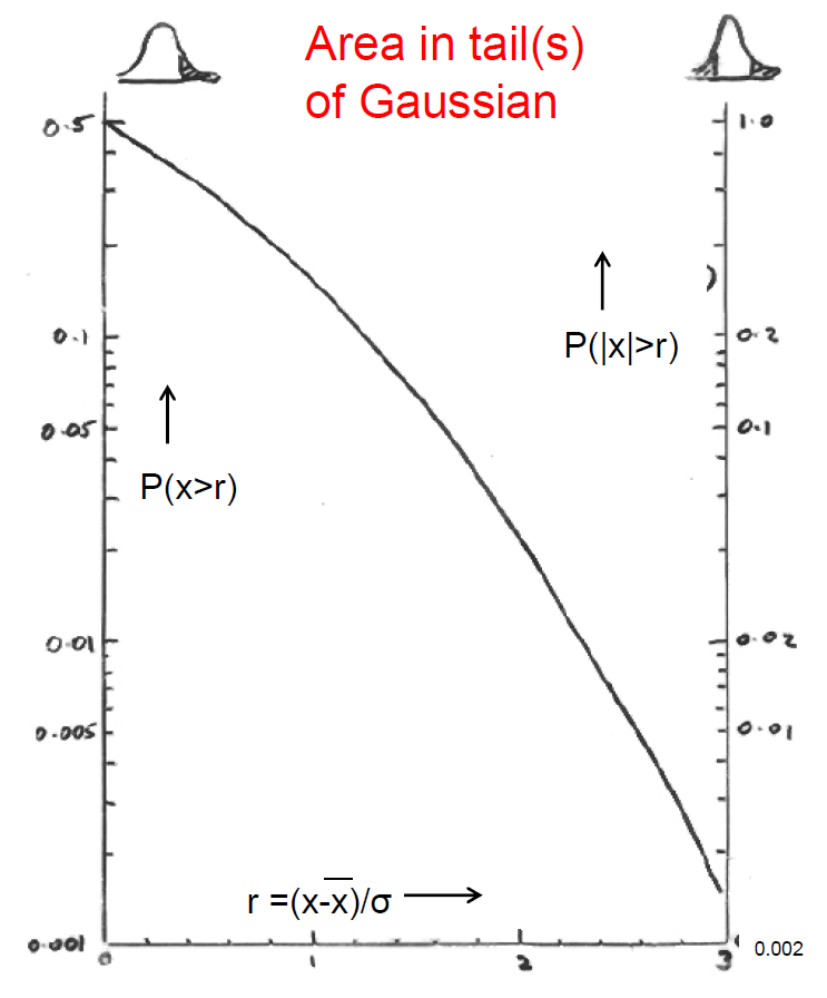
Figure 4: The fractional area in the tail(s) of a Gaussian distribution i.e. the area with $f$ above some specified value $r$, where $f$ is the distance from the mean, measured in units of the standard deviation $\sigma$. The scale on the left refers to the one-sided tail, while that on the right is for both tails. Thus for $r=0$, the fractional areas are 1/2 and 1 respectively.

For deciding whether an experimental measurement is consistent with a theory, more useful than the Gaussian distribution itself is its tail area beyond $r$, a number of standard deviations from the central value (see Fig. 4). This gives the probability of obtaining a result as extreme as ours or more so as a consequence of statistical fluctuations, assuming that the theory is correct (and that our measurement is unbiassed, it is Gaussian distributed, etc.). If this probability is small, the measurement and the theory may be inconsistent.

Figure 4 has two different vertical scales, the left one for the probability of a fluctuation in a specific direction, and the right side for a fluctuation in either direction. Which to use depends on the particular situation. For example if we were performing a neutrino oscillation disappearance experiment, we would be looking for a reduction in the number of events as compared with the no-oscillation scenario, and hence would be interested in just the single-sided tail. In contrast searching for any deviation from the Standard Model expectation, maybe the two-sided tails would be more relevant.

12 Introduction to Lecture 2

This lecture deals with two different methods for determining parameters, least squares and likelihood, when a functional form is fitted to our data. A simple example would be straight line fitting, where the parameters are the intercept and gradient of the line. However the methods are much more general than this. Also there are other methods of extracting parameters; these include the more fundamental Bayesian and Frequentist methods, which are dealt with in Lecture 3 .

The least squares method also provides a measure of Goodness of Fit for the agreement between the theory with the best values of the parameters, and the data; this is dealt with in section 14. The likelihood technique plays an important role in the Bayes approach, and likelihood ratios are relevant for choosing between two hypotheses; this is covered in Lecture 4.

13 Least squares: Basic idea

As a specific example, we will consider fitting a straight line $y=a+bx$ to some data, which consist of a series on $n$ data points, each of which specifies $(x_{i},y_{i}\pm\sigma_{i})$ i.e. at precisely known $x_{i}$, the $y$ co-ordinate is measured with an uncertainty $\sigma_{i}$. The $\sigma_{i}$ are assumed to be uncorrelated. The more general case could involve

• a more complicated functional form than linear;

• multidimensional $x$ and/or $y$;

• correlations among the $\sigma_{i}$; and

• uncertainties on the $x_{i}$ values.

In Particle Physics, we often deal with a histogram of some physical quantity $x$ (e.g. mass, angle, transverse momentum, etc.), in which case $y$ is simply the number of counts for that $x$ bin. Another possiblity is that $y$ and $x$ are both physical quantities e.g. we have a two-dimensional plot showing the recession velocities of galaxies as a function their distance.

There are two statistical issues: Are our data consistent with the theory i.e. a straight line? And what are the best estimates of the parameters, the intercept and the gradient? The former is a Goodness of Fit issue, while the latter is Parameter Determination. The Goodness of Fit is more fundamental, in that if the data are not consistent with the hypothesis, the parameter values are meaningless. However, we will first consider Parameter Detemination, since checking the quality of the fit requires us to use the best straight line.

The data statistic used for both questions is $S$, the weighted sum of squared discrepancies

$$S=\Sigma(y_{i}^{th}-y_{i}^{obs})^{2}/\sigma_{i}^{2}=\Sigma(a+bx_{i}-y_{i}^{obs})^{2}/\sigma_{i}^{2}$$ (25)

where $y_{i}^{th}=a+bx_{i}$ is the predicted value of $y$ at $x_{i}$, and $y_{i}^{obs}$ is the observed value. In the expression for $S$, we regard the data $(x_{i},y_{i}\pm\sigma_{i})$ as being fixed, and the parameters $a$ and $b$ as being variable. If for specific values of $a$ and $b$ the predicted values of $y$ and the corresponding observed ones are all close (as measured in terms of the uncertainties $\sigma$), then $S$ will be ‘small’, while significant discrepancies result in large $S$. Thus, according to the least squares method, the best values of the parameters are those that minimise $S$, and the width of the $S$ distribution determines their uncertainties. For a good fit, the value of $S_{min}$ should be ‘small’. A more quantative discussion of ‘small’ appears below.

To determine the best values of $a$ and $b$, we need to set the first derivatives of $S$ with respect to $a$ and $b$ both equal to zero. This leads to two simultaneous linear equations for $a$ and $b$ which are readily solved, to yield

$$\begin{split}a&=\frac{<x^{2}><y>-<xy><x>}{<x^{2}>-<x>^{2}}\\ b&=\frac{<xy>-<x><y>}{<x^{2}>-<x>^{2}}\end{split}$$ (26)

where $<f>\ =\Sigma(f_{i}/\sigma_{i}^{2})/\Sigma(1/\sigma_{i}^{2})$ i.e it is the weighted average of the quantity inside the brackets. If the positions of the data points are such that $<x>\ =0$, then $a=\ <y>$, i.e. the height of the best fit line at the weighted centre of gravity of the data points is just the weighted average of the $y$ values.

It is also essential to calculate the uncertainties $\sigma_{a}$ and $\sigma_{b}$ on the parameters and their correlation coefficient $\rho=cov/(\sigma_{x}\sigma_{y})$, where $cov$ is their covariance. The elements of the inverse covariance matrix $M$ are given by

$$\begin{split}M_{aa}&=\frac{1}{2}\frac{\partial^{2}S}{\partial a^{2}}=\Sigma(1/\sigma_{i}^{2})\\ M_{ab}&=\frac{1}{2}\frac{\partial^{2}S}{\partial a\ \partial b}=\Sigma(x_{i}/\sigma_{i}^{2})\\ M_{bb}&=\frac{1}{2}\frac{\partial^{2}S}{\partial b^{2}}=\Sigma(x_{i}^{2}/\sigma_{i}^{2})\\ \end{split}$$ (27)

The covariance matrix is obtained by inverting $M$. Since the covariance is proportional to $-<x>$, if the data are centred around $x=0$, the uncertainties on $a$ and $b$ will be uncorrelated. That is one reason why track parameters are usually specified at the centre of the track, rather than at its starting point.

13.1 Correlated uncertainties on data

So far we have considered that the uncertainties on the data are uncorrelated, but this is not always the case; correlations can arise from some common systematic. Then instead of the first equation of (25), we use

$$S=\Sigma\Sigma(y_{i}^{th}-y_{i}^{obs})E_{ij}(y_{j}^{th}-y_{j}^{obs})$$ (28)

where the double summation is over $i$ and $j$, and $E$ is the inverse covariance matrix for the uncertainties on the $y_{i}$. For the special case of uncorrelated uncertainties, the only non-zero elements of $E$ are the diagonal ones $E_{ii}=1/\sigma_{i}^{2}$ and then eqn. (28) reduces to (25).

This new equation for $S$ can then be minimised to give the best values of the parameters, and $S_{min}$ can be used in a Goodness of Fit test. As before, if $y^{th}$ is linear in the parameters, their best estimates can be obtained by solving simultaneous linear equations, without the need for a minimisation programme.

14 Least squares for Goodness of Fit

14.1 The chi-squared distribution

It turns out that, if we repeated our experiment a large number of times, and certain conditions are satisfied, then $S_{min}$ will follow a $\chi^{2}$ distribution with $\nu=n-p$ degrees of freedom, where $n$ is the number of data points, $p$ is the number of free parameters in the fit, and $S_{min}$ is the value of $S$ for the best values of the free parameters. For example, a straight line with free intercept and gradient fitted to 12 data points would have $\nu=10$.

The conditions for this to be true include:

• the theory is correct:

• the data are unbiassed and asymptotic;

• the $y_{i}$ are Gaussian distributed about their true values;

• the estimates for $\sigma_{i}$ are correct;           etc.

Useful properties to know about the mathematical $\chi^{2}$ distribution are that their mean is $\nu$ and their variance is $2\nu$. Thus if a global fit to a lot of data has $S_{min}$ = 2200 and there are 2000 degrees of freedom, we can immediately estimate that this is equivalent to a fluctuation of 3.2$\sigma$.

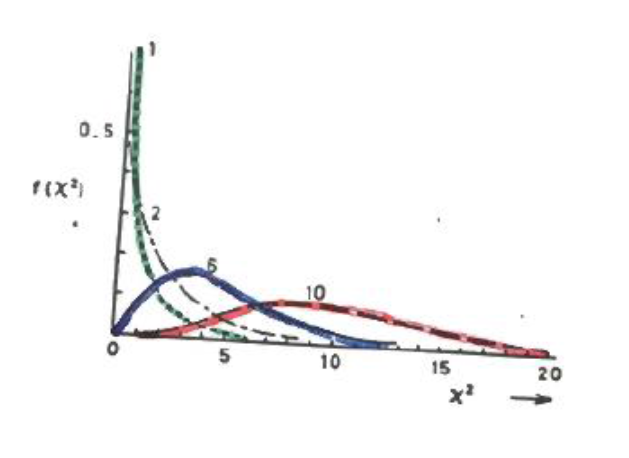
Figure 5: Mathematical distributions of $\chi^{2}$, for different numbers of degrees of freedom $\nu$ (shown beside each curve). As $\nu$ increases, so do the mean and variance of the distribution.

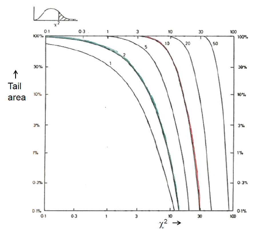
Figure 6: The percentage area in the upper tails of $\chi^{2}$ distributions, for various numbers of degrees of freedom, shown by each curve. Both scales are logarithmic. These curves bear the same relationship to those of figure 5 as does fig. 4 to the Gaussian of fig. 3, both in Lecture 1.

More useful than plots of $\chi^{2}$ distributions are those of the fractional tail area beyond a particular value of $\chi^{2}$ (see figs. 5 and 6 respectively). The $\chi^{2}$ goodness of fit test consists of

• For the given theoretical form, find the best values of its free parameters, and hence $S_{min}$;

• Determine $\nu$ from $n$ and $p$; and

• Use $S_{min}$ and $\nu$ to obtain the tail probability $p$ .

Then $p$ is the probability that, if the theory is correct, by random fluctuations we would have obtained a value of $S_{min}$ at least as large as the observed one. If this probability is smaller than some pre-defined level $\alpha$, we reject the hypothesis that the model provides a good description of the data.

14.2 When $\nu\neq n-p$

If we add an extra parameter into our theoretical description, even if it is not really needed, we expect the value of $S_{min}$ to decrease slightly. (This contrasts with including a parameter which is really relevant, which can result in a dramatic reduction in $S_{min}$.) In determining $p$-values, this is allowed for by the reduction of $\nu$. On average, a parameter which is not needed reduces $S_{min}$ by 1. But consider the following examples.

14.2.1 Small oscillatory term

Imaging we are fitting a histogram of a variable $\phi$ by a distribution of the form

$$\frac{dy}{d\phi}=N[1+10^{-6}cos(\phi-\phi_{0})],$$ (29)

where the two parameters are the normaisation $N$ and the phase $\phi_{0}$. Because of the factor $10^{-6}$ in front of the cosine term, $\phi_{0}$ will have a miniscule effect on the prediction, and so including this as a parameter has negligible effect on $S_{min}$; $\phi_{0}$ is effectively not a free parameter.

14.2.2 Neutrino oscillations

For a scenario of two oscillating neutrino flavours, the probability $P$ of a neutrino of energy $E$ to remain the same flavour after a flight length $L$ is

$$P=1-Asin^{2}(\delta m^{2}L/E)$$ (30)

where the two parameters are $\delta m^{2}$, the difference in the mass-squareds of the two neutrino flavours, and $A=sin^{2}2\theta$ with $\theta$ being the mixing angle. However, since for small angles $\alpha,\ sin\alpha\approx\alpha$, for small $\delta m^{2}L/E$ the probability $P$ of eqn 30 is approximately $1-A(\delta m^{2}L/E)^{2}$. Thus the two parameters occur only as the product $A(\delta m^{2})^{2}$, and cannot be determined separately. Thus in that regime we have effectively just a single parameter.

In both the above examples, an enormous amount of data would enable us to distinguish the small effects produced by the second parameter; hence the requirement for asymptotic conditions.

14.3 Errors of First and Second Kind

In deciding in a Goodness of Fit test whether or not to reject the null hypothesis $H_{0}$ (e.g. that the data points lie on a straight line), there are two sorts of mistake we might make:

• Error of the First Kind. This is when we reject $H_{0}$ when it is in fact true. The fraction of cases in which this happens should equal $\alpha$, the cut on the $p$-value.

• Error of the Second Kind. This is when we do not reject $H_{0}$, even though some other hypothesis is true. The rate at which this happens depends on how similar $H_{0}$ and the alternative hypothesis are, the relative frequencies of the two hypotheses being true, etc.

As $\alpha$ increases the rates of Errors of the First and Second kinds go up and down respectively. These Errors correspond to a loss of efficiency and to an increase of contamination respectively.

14.4 Other Goodness of Fit tests

The $\chi^{2}$ method is by no means the only one for testing Goodness of Fit. Indeed whole books have been written on the subject[6]. Here we mention just one other, the Kolmogorov-Smirnov method (K-S), which has the advantage of working with individual observations. It thus can be used with fewer observations than are required for the binned histograms in the $\chi^{2}$ approach.

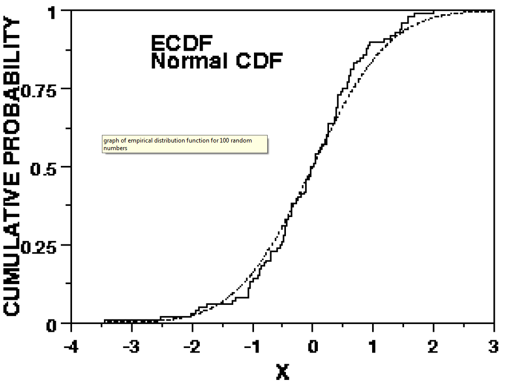
Figure 7: Cumulative distributions for the Kolmogorov-Smirnov goodness of fit method. The stepped distribution shows the fraction of events in a data sample, while the continuous curve is that expected for a Gaussian with mean zero and unit variance. The method uses the maximum vertical separation $d$ between the two distributions, and the number of observations, to obtain the probability of obtaining a value of $d$ at least as large as the observed one. A small probability implies that it is unlikely that the data sample comes from the assumed distribution.

A cumulative plot is produced of the fraction of events as a function of the variable of interest $x$. An example is shown in Fig. 7. This shows the fraction of data events with $x$ smaller than any particular value. It is thus a stepped plot, with the fraction going from zero at the extreme left, to unity on the right hand side. Also on the plot is a curve showing the expected cumulative fraction for some theory. The K-S method makes use of the largest (as a function of $x$) vertical discrepancy $d$ between the data plot and the theoretical curve. Assuming the theory is true and given the number of observations $N$, the probability $p_{KS}$ of obtaining $d$ at least as large as the observed value can be calculated. The beauty of the K-S method is that this probability is independent of the details of the theory. As in the $\chi^{2}$ approach, the K-S probability gives a numerical way of checking the compatibility of theory and data. If $p_{KS}$ is small, we are likely to reject the theory as being a good description of the data.

Some features of the K-S method are:

• The main advantage is that it can use a small number of observations.

• The calculation of the K-S probability depends on there being no adjustable parameters in the theory. If there are, it will be necessary for you to determine the expected distribution for $d$, presumably by Monte Carlo simulation.

• It does not extend naturally to data of more than one dimension, because of there being no unique way of producing an ordering in several dimensions.

• It is not very sensitive to deviations in the tails of distributions, which is where searches for new physics are often concentrated e.g. high mass or transverse momentum. Fortunately variants of K-S exist, which put more emphasis on discrepancies in the tails.

• Instead of comparing a data cumulative distribution with a theoretical curve, it can alternatively be compared with another distribution. This can be from a simulation of a theory, or with another data set. The latter could be to check that two data sets are compatible. The calculation of the K-S probability now requires the maximum discrepancy $d$, and the numbers of events $N_{1}$ and $N_{2}$ in each of the two distributions being compared.

15 Kinematic Fitting

Earlier we had the example of estimating the number of married people on an island, and saw that introducing theoretical information could improve the accuracy of our answer. Here we use the same idea in the context of estimating the momenta and directions of objects produced in a high energy interaction. The theory we use is that energy and momentum are conserved between the inital state collison and the observed objects in the reaction.

The reaction can be either at a collider or with a stationary target. We denote it by $a+b\rightarrow c+d+e$, but the number of final state objects can be arbitrary. We assume for the time being the energy and momenta of all the objects are measured.

The technique is to consider all possible configurations of the particles’ kinematic variables that conserve momentum and energy, and to choose that configuration that is closest to the measured variables. The degree of closeness is defined by the weighted sum of squares of the discrepancies $S$, taking the uncertainties and correlations into account. If the uncertainties on the kinematic quantities $m_{i}$ were uncorrelated,

$$S=\Sigma(f_{i}-m_{i})^{2}/\sigma_{i}^{2}$$ (31)

where the summation is over the 4 components for all the objects in the reaction, $m_{i}$ are the measured values and $f_{i}$ are the corresponding fitting quantities. Because of correlations, however, this becomes

$$S=\Sigma\Sigma(f_{i}-m_{i})E_{ij}(f_{j}-m_{j})$$ (32)

where there is now a double summation over the components, and $E_{ij}$ is the $(i,j)^{th}$ component of the inverse covariance matrix for the measured quantities. The procedure then consists in varying $f$ in order to minimise $S$, subject to the energy and momentum constraints. This usually involves Lagrange Multipliers. The result of this procedure is to produce a set of fitted values of all the kinematic quantities, which will have smaller uncertainties than the measured ones. This is an example of incorporating theory to improve the results. Thus if the objects are jets, their directions are usually quite well determined, but their energies less so. The fitting procedure enables the accurately determined jet directions to help reduce the uncertainties on the jet energies.

The fitting procedure also provides $S_{min}$, which is a measure of how well the best $f_{i}$ agree with the $m_{i}$. In the case described, the distribution of $S_{min}$ is approximately $\chi^{2}$ with 4 degrees of freedom (because of the 4 constraints).

If $S_{min}$ is too large, then our assumed hypothesis for the reaction may be incorrect; for example, there might have been an extra object produced in the collision that was undetected (e.g. a neutrino, or a charged particle which passed through an uninstrumented region of our detector).

Since we have 4 constraint equations, we can also allow for up to 4 missing kinematic quantities. Examples include an undetected neutrino in the final state (3 unmeasured momentum components), a wide-band neutrino beam of known direction (1 missing variable), etc. With $m$ missing variables in an interaction involving a single vertex, $S_{min}$ should have a $\chi^{2}$ distribution with $4-m$ degrees of freedom.

Kinematic fitting can be extended to more complicated event topologies including production and decay vertices, reactions involving particles of well known mass which decay promptly (e.g. $\psi\rightarrow\mu^{+}\mu^{-}$), etc.

15.1 Example of a simplified kinematic fit

Consider a non-relativistic elastic scattering of two equal mass objects, for example a slow anti-proton hitting a stationary proton. For simplicity, the measured angles $\theta_{1}^{m}\pm\sigma$ and $\theta_{2}^{m}\pm\sigma$ that the outgoing particles make with the direction of travel of the incident anti-proton are assumed to have the same uncorrelated uncertainties $\sigma$. As a result of energy and momentum conservation, the angles must satisfy the constraint

$$\theta_{1}^{t}+\theta_{2}^{t}=\pi/2$$ (33)

where the superscipt $t$ denotes the true value. There are 3 further constraints but for simplicity we shall ignore them.

To find our best estimates of $\theta_{1}^{t}$ and $\theta_{2}^{t}$, we must minimise

$$S=(\theta_{1}^{t}-\theta_{1}^{m})^{2}/\sigma^{2}+(\theta_{2}^{t}-\theta_{2}^{m})^{2}/\sigma^{2}$$ (34)

subject to the constraint 33. By using Lagrange Multipliers or by eliminating $\theta_{2}^{t}$ and then minimising $S$, this yields

$$\begin{split}\theta_{1}^{t}&=\theta_{1}^{m}+0.5*(\pi/2-\theta_{1}^{m}-\theta_{2}^{m})\\ \theta_{2}^{t}&=\theta_{2}^{m}+0.5*(\pi/2-\theta_{1}^{m}-\theta_{2}^{m})\end{split}$$ (35)

That is, the best estimate of each true value is obtained by adding to the corresponding measured value half the amount by which the measured values fail to satisfy the constraint 33.

The uncertainties on the fitted estimates of the angles are easily obtained by propagation of the uncertainties $\sigma$ on the measured angles vias eqns. 35, and are both equal to $\sigma/\sqrt{2}$.

We thus have an example of the promised outcome that kinematic fitting improves the accuracy of our measurements. The factor of $\sqrt{2}$ improvement can easily be understood in that we have two independent estimates of $\theta_{1}^{t}$, the first being the original measurement $\theta_{1}^{m}$, and the other coming from the measurement $\theta_{2}^{m}$ via the constraint 33. However, even with uncorrelated uncertainties on the measured angles, the fitted ones would be anti-correlated.

16 THE paradox

I refer to this as ‘THE’ paradox as, in various forms, it is the basis of the most frequently asked question.

You have a histogram of 100 bins containing some data, and use this to determine the best value $\mu_{0}$ of a parameter $\mu$ by the $\chi^{2}$ method. It turns out that $S_{min}=87$, which is reasonable as the expected value for a $\chi^{2}$ with 99 degrees of freedom is $99\pm 14$. A theorist asks whether his predicted value $\mu_{th}$ is consistent with your data, so you calculate $S(\mu_{th})$ = 112. The theorist is happy because this is within the expected range. But you point out that the uncertainty in $\mu$ is calculated by finding where $S$ increases by 1 unit from its minimum. Since 112 is 25 units larger than 87, this is equivalent to a 5 standard deviation discrepancy, and so you rule out the theorist’s value of $\mu$.

Deciding which viewpoint is correct is left as an excercise for the reader.

17 Likelihood

The likelihood function is very widely used in many statistics applications. In this Section, we consider it just for Parameter Determination. An important feature of the likelihood approach is that it can be used with unbinned data, and hence can be applied in situations where there are not enough individual observations to construct a histogram for the $\chi^{2}$ approach.

We start by assuming that we wish to fit our data $x$, using a model $f(x;\mu)$ which has one or more free parameters $\mu$, whose value(s) we need to determine. The function $f$ is known as the ‘probability distribution’ ($pdf$) and specifies the probability (or probability density, for the data having continuous as opposed to discrete values) for obtaining different values of the data, when the parameter(s) are specified. Without this it is impossible to apply the likelihood (or many other) approaches. For example $x$ could be observations of a variable of interest within some range, and $f$ could be any function such as a straight line, with gradient and intercept as parameters. But we will start with an angular distribution

$$y(\cos\theta;\beta)=\frac{d\ p}{d\cos\theta}=N(1+\beta\cos^{2}\theta)$$ (36)

Here $\theta$ is the angle at which a particle is observed, $dp/d\cos\theta$ is the $pdf$ specifying the probability density for observing a decay at any $\cos\theta$, $\beta$ is the parameter we want to determine, and $N$ is the crucial nomalisation factor which ensures that the probability of observing a given decay at any $\cos\theta$ in the whole range from $-1$ to $+1$ is unity. In this case $N=1/(2(1+\beta/3))$. The data consists of $N$ decays, with their individual observations $\cos\theta_{i}$.

Assuming temporarily that the value of the parameter $\beta$ is specified, the probability density $y_{1}$ of observing the first decay at $\cos\theta_{1}$ is

$$y_{1}=N(1+\beta\cos^{2}\theta_{1})=0.5(1+\beta\cos^{2}\theta_{1})/(1+\beta/3),$$ (37)

and similarly for the rest of the $N$ observations. Since the individual observations are independent, the overall probability $P(\beta)$ of observing the complete data set of $N$ events is given by the product of the individual probabilities

$$P(\beta)=\Pi y_{i}=\Pi\ 0.5(1+\beta\cos^{2}\theta_{i})/(1+\beta/3)$$ (38)

We imagine that this is computed for all values of the parameter $\beta$; then this is known as the likelihood function ${\it L}(\beta)$.

The likelihood method then takes as the estimate of $\beta$ that value which maximises the likelihood. That is, it is the value which maximises (with respect to $\beta$) the probability density of observing the given data set. Conversely we rule out values of $\beta$ for which ${\it L}(\beta)$ is very small. The uncertainty on $\beta$ is related to the width of the ${\it L}(\beta)$ distribution (see later).

It is often convenient to consider the logarithm of the likelihood

$${\it l}=\ln{\it L}=\Sigma\ln y_{i}$$ (39)

One reason for this is that, for a large number of observations some fraction could have small $y_{i}$. Then the likelihood, involving the product of the $y_{i}$, could be very small and may underflow the computer’s range for real numbers. In contrast, l involves a sum rather than a product, and $\ln y_{i}$ rather than $y_{i}$, and so produces a gentler number.

17.1 Likelihood and $pdf$

The procedure for constructing the likelihood is first to write down the $pdf$, and then to insert into that expression the observed data values in order to evaluate their product, which is the likelihood. Thus both the $pdf$ and the likelihood involve the data $x$ and the parameter(s) $\mu$. The difference is that the $pdf$ is a function of $x$ for fixed values of $\mu$, while the likelihood is a function of $\mu$ given the fixed observed data $x_{obs}$.

Thus for a Poisson distribution, the probability of observing $n$ events when the rate $\mu$ is specified is

$$P(n;\mu)=e^{-\mu}\mu^{n}/n!$$ (40)

and is a function of $n$, while the likelihood is

$$L(\mu;n)=e^{-\mu}\mu^{n}/n!$$ (41)

and is a function of $\mu$ for the fixed observed number $n$.

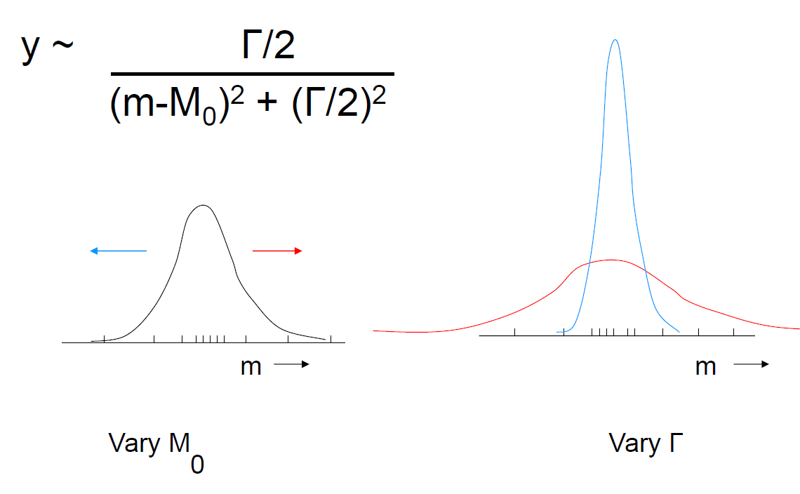
Figure 8: A visual demonstration of how the maximum likelihood method gives sensible values for the parameters, the position and width of a resonance. The bars along the $m$-axis represent the experimental measurements of a set of mass values $m_{i}$, which are to be fitted by a simple Breit-Wigner resonance shape. In (a), the width $\Gamma$ of the resonance is kept fixed, and the mass parameter $M_{0}$ is varied. This has the effect of sliding the curve to the left or right along the $m$-axis, without changing its shape or height. To calculate the likelihood for a given position of the curve we multiply all the $y(m_{i})$ values; i.e. the height of the curve at each observed mass. The best value of $M_{0}$ is thus equivalent to finding the best location of the curve in order to maximise this product. Clearly we need to locate the peak near where most of the data values are. In (b), we regard $M_{0}$ as constant, but vary the width. The effect of the normalisation condition then means that the wider curve will have lower peak height and vice versa. The narrow curve suffers becase of the very small $y$ values for the extreme observed mass values, while wide curves do not benefit so much from the concentration of masses around the central value. The best value of $\Gamma$ is the result of a compromise between these two effects.

17.2 Intuitive example: Location and width of peak

We consider a situation where we are studying a resonant state which would result in a bump in the mass distribution of its decay particles. We assume that the bump can be parametrised as a simple Breit-Wigner

$$y(m;M_{0},\Gamma)=\frac{\Gamma/(2\pi)}{(m-M_{0})^{2}+(\Gamma/2)^{2}}$$ (42)

where $y$ is the probability density of obtaining a mass $m$ if the location and width the state are $M_{0}$ and $\Gamma$, the parameters we want to determine. It is essential that $y$ is normalised, i.e. its integral over all physical values of $m$ is unity; hence the normalisation factor of $\Gamma/(2\pi)$. The data consists of $n$ observations of $m$, as shown in fig. 8.

Assume for the moment that we know $M_{0}$ and $\Gamma$. Then the probability density for observing the $i^{th}$ event with mass $m_{i}$ is

$$y_{i}(M_{0},\Gamma)=\frac{\Gamma/(2\pi)}{(m_{i}-M_{0})^{2}+(\Gamma/2)^{2}}$$ (43)

Since the events are independent, the probability density for observing the whole data sample is

$$y_{all}(M_{0},\Gamma)=\Pi\ \frac{\Gamma/(2\pi)}{(m_{i}-M_{0})^{2}+(\Gamma/2)^{2}}$$ (44)

and this is known as the likelihood $L(M_{0},\Gamma)$. Then the best values for the parameters are taken as the combination that maximises the probability density for the whole data sample i.e. $L(M_{0},\Gamma)$. Parameter values for which $L$ is very small compared to its maximum value are rejected, and the uncertainties on the parameters are related to the width of the distribution of $L$; we will be more specific later.

The curve in fig. 8(left) shows the expected probability distribution for fixed parameter values. The way $L$ is calculated involves multiplying the heights of the curve at all the observed $m_{i}$ values. If we now consider varying $M_{0}$, this moves the curve bodily to the left or right without changing its shape or normalisation. So to determine the best value of $M_{0}$, we need to find where to locate the curve so that the product of the heights is a maximum; it is plausibe that the peak will be located where the majority of events are to be found.

Now we will consider how the optimum value of $\Gamma$ is obtained. A small $\Gamma$ results in a narrow curve, so the masses in the tail will make an even smaller contribution to the product in eqn. 44, and hence reduce the likelihood. But a large $\Gamma$ is not good, because not only is the width larger, but because of the normalisation condition, the peak height is reduced, and so the observations in the peak region make a smaller contribution to the likelihood. The optimal $\Gamma$ involves a trade-off between these two effects.

Of course, in finding the optimal of values of the two parameters, in general it is necessary to find the maximum of the likelihood as a function of the two parameters, rather than maximising with respect to just one, and then with respect to the other and then stopping (see section 17.5).

17.3 Uncertainty on parameter

With a large amount of data, the likelihood as a function of a parameter $\mu$ is often approximately Gaussian. In that case, ${\it l}$ is an upturned parabola. Then the following definitions of $\sigma_{\mu}$, the uncertainty on $\mu_{best}$, yield identical answers:

• The RMS of the likelihood distribution.

• [$-\frac{d^{2}{\it l}}{d\mu^{2}}]^{-1/2}$. If you remember that the second derivative of the log likelihood function is involved because it controls the width of the ${\it l}$ distribution, a mneumonic helps you remember the formula for $\sigma_{\mu}$: Since $\sigma_{\mu}$ must have the same units as $\mu$, the second derivative must appear to the power $-1/2$. But because the log of the likelihood has a maximum, the second derivative is negative, so the minus sign is necessary before we take the square root.

• It is the distance in $\mu$ from the maximum in order to decrease ${\it l}$ by half a unit from its maximum value. i.e.

  $${\it l}(\mu_{best}+\sigma_{\mu})={\it l}_{max}-0.5$$ (45)

In situations where the likelihood is not Gaussian in shape, these three definitions no longer agree. The third one is most commonly used in that case. Now the upper and lower ends of the intervals can be asymmetric with respect to the central value. It is a mistake to believe that this method provides intervals which have a $68\%$ chance of containing the true value of the parameter.

Symmetric uncertainties are easier to work with than asymmetric ones. It is thus sometimes better to quote the uncertainty on a function of the first variable you think of. For example, for a charged particle in a magnetic field, the reciprocal of the momentum has a nearly symmetric uncertainty. Especially for high momentum tracks, the upper uncertainty on the momentum can be much larger than the lower one e.g. $1.0\ ^{+1.5}_{-0.4}$ TeV.

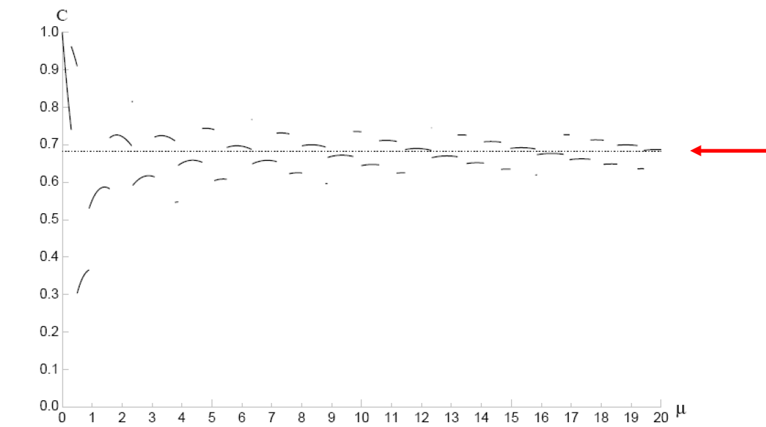
Figure 9: Coverage C for Poisson parameter intervals, as determined by the $\Delta(log(L))=0.5$ rule. Repeated trials (all using the same Poisson parameter $\mu$) yield different values of $n$, each resulting in its own range $\mu_{l}$ to $\mu_{u}$ for $\mu$; then C is the fraction of trials that give ranges which include the chosen value of $\mu$ for the trials. The coverage C varies with $\mu$, and has discontinuities because the data $n$ can take on only discrete integer values. For large $\mu$, C seems to approach the expected 0.68, shown by the arrow, but for small $\mu$, the coverage takes on values between $30\%$ and $100\%$.

17.4 Coverage

An important feature of any statistical method for estimating a range for some parameter $\mu$ at a specified confidence level $\alpha$ is its coverage $C$. If the procedure is applied many times, these ranges will vary because of statistical fluctuations in the observed data. Then $C$ is defined as the fraction of ranges which contain the true value $\mu_{true}$; it can vary with $\mu_{true}$.

It is very important to realise that coverage is a property of the statistical procedure and does not apply to your particular measurement. An ideal plot of coverage as a function of $\mu$ would have $C$ constant at its nominal value $\alpha$. For a Poisson counting experiment, figure 9 shows $C$ as a function of the Poisson parameter $\mu$, when the observed number of counts $n$ is used to determine a range for $\mu$ via the change in log-likelihood being 0.5. The coverage is far from constant at small $\mu$. If $C$ is smaller than $\alpha$, this is known as undercoverage. Certainly frequentists would regard this as unfortunate; it means that people reading an article containing parameters determined this way are likely to place more than justified reliance on the quoted range. Methods using the Neyman construction to determine parameter ranges by construction do not have undercoverage.

Coverage involves a statement about $Prob[\mu_{l}\leq\mu_{true}\leq\mu_{u}]$. This is to be interpreted as a probability statement about how often the ranges $\mu_{l}$ to $\mu_{u}$ contain the (unknown but constant) true value $\mu_{true}$. This is a frequentist statement; Bayesians do not want to consider the ensemble of possible results if the measurement procedure were to be repeated. Thus Bayesians would regard the statement about $Prob[\mu_{l}\leq\mu_{true}\leq\mu_{u}]$ as describing what fraction of their estimated posterior probability density for $\mu_{true}$ would be between the fixed values $\mu_{l}$ and $\mu_{u}$, derived from their actual measurement.

17.5 More than one parameter

For the case of just one parameter $\mu$, the likelihood best estimate $\hat{\mu}$ is given by the value of $\mu$ which maximises $L$. Its uncertainty $\sigma_{\mu}$ is determined either from

$$1/\sigma_{\mu}^{2}=-d^{2}\ln L/d\mu^{2};$$ (46)

of by finding how far $\hat{\mu}$ would have to be changed in order to reduce $\ln L$ by 0.5.

When we have two or more parameters $\beta_{i}$ the rule for finding the best estimates $\hat{\beta_{i}}$ is still to maximise $L$. For the uncertainties and their correlations, the generalisation of equation 46 is to construct the inverse covariance matrix ${\bf M}$, whose elements are given by

$$M_{ij}=-\frac{\partial^{2}\ln L}{\partial\beta_{i}\ \partial\beta_{j}}$$ (47)

Then the inverse of $\bf{M}$ is the covariance matrix, whose diagonal elements are the variances of $\beta_{i}$, and whose off-diagonal ones are the covariances.

Alternatively (and more common in practice), the uncertainty on a specific $\beta_{j}$ can be obtained by using the profile likelihood $L_{prof}(\beta_{j})$. This is the likelihood as a function of the specific $\beta_{j}$, where for each value of $\beta_{j},\ L$ has been remaximised with respect to all the other $\beta$. Then $L_{prof}(\beta_{j})$ is used with the ‘reduce $\ln L_{prof}$ = 0.5’ rule to obtain the uncertainty on $\beta_{j}$. This is equivalent to determining the contour in $\beta$-space where $\ln L=\ln L_{max}-0.5$, and finding the values $\beta_{j,1}$ and $\beta_{j,2}$ on the contour which are furthest from $\hat{\beta_{j}.}$ Then the (probably asymmetric) upper and lower uncertainties on $\beta_{j}$ are given by $\beta_{j,2}-\hat{\beta_{j}}$ and $\hat{\beta_{j}}-\beta_{j,1}$ respectively.

Because these are likelihood methods of obtaining the intervals, these estimates of uncertainities provide only nominal regions of 68% coverage for each parameter; the actual coverage can differ from this. Furthermore, the region within the contour described in the previous paragraph for the multidimensional $\beta$ space will have less than 68% nominal overage. To achieve that, the $`0.5^{\prime}$ in the rule for how much $\ln L$ has to be reduced from its maximum must be replaced by a larger number, whose value depends on the dimensionality of $\beta$.

18 Worked example: Lifetime determination

Here we consider an experiment which has resulted in $N$ observed decay times $t_{i}$ of a particle whose lifetime $\tau$ we want to determine. The probability density for observing a decay at time $t$ is

$$p(t;\tau)=(1/\tau)\ e^{-t/\tau}$$ (48)

Note the essential normalisation factor $1/\tau$; without this the likelihood method does not work.

It should be realised that realistic situations are more complicated than this. For example, we ignore the possibility of backgrounds, time resolution which smears the expected values of $t$, acceptance or efficiency effects which vary with $t$, etc., but this enables us to estimate $\tau$ and its uncertainty $\sigma_{\tau}$ analytically. In real practical cases, it is almost always necessary to calculate the likelihood as a function of $\tau$ numerically.

From equation 48 we calculate the log-likelihood as

$$\ln L(\tau)=\ln[\Pi\ (1/\tau)e^{-t_{i}/\tau}]\ \ =\ \ \Sigma(-\ln\tau-t_{i}/\tau)$$ (49)

Differentiating $\ln L(\tau)$ with respect to $\tau$ and setting the derivative to zero then yields

$$\tau=\Sigma t_{i}/N$$ (50)

This equation has an appealing feature, as it can be read as “The mean lifetime is equal to the mean lifetime", which sounds as if it must be true. However, what it really says is not quite so trivial: “Our best estimate of the lifetime parameter $\tau$ is equal to the mean of the $N$ observed decay times in our experiment."

We next calculate $\sigma_{\tau}$ from the second derivative of $\ln L$, and obtain

$$\sigma_{\tau}=\tau/\sqrt{N}$$ (51)

This exhibits a common feature that the uncertainty of our parameter estimate decreases as $1/\sqrt{N}$ as we collect more and more data. However, a potential problem arises from the fact that our estimated uncertainty is proportional to our estimate of the parameter. This is relevant if we are trying to combine different experimental results on the lifetime of a particle. For combining procedures which weight each result by $1/\sigma^{2}$, a measurement where the fluctuations in the observed times result in a low estimate of $\tau$ will tend to be over-weighted (compare the section on ‘Combining Experiments’ in Lecture 1), and so the weighted average would be biassed downwards. This shows that it is better to combine different experiments at the data level, rather than simply trying to use their results.

One final point to note about our simplified example is that the likelihood $L(\tau)$ depends on the observations only via the sum of the times $\Sigma t_{i}$ i.e. their distribution is irrelevant. Thus the likelihood distributions for two experiments having the same number of events and the same sum of observed decay times, but with one having the decay times consistent with an exponential distribution and the other having something completely different (e.g. all decays occur at the same time), would have identical likelihood functions. This provides an example of the fact that the unbinned likelihood function does not in general provide useful information on Goodness of Fit.

19 Conclusions

Jut as it is impossible to learn to play the violin without ever picking it up and spending hours actually using it, it is important to realise that one does not learn how to apply Statistics merely by listening to lectures. It is really important to work through examples and actual analyses, and to discover more about the topics.

There are many resources that are available to help you. First there are textbooks written by Particle Physicists[8], which address the statistical problems that occur in Particle Physics, and which use a language which is easier for other Particle Physicists to understand.

The large experimental collaborations have Statistics Committees, whose web-sites contain lots of useful statistical information. That of CDF[9] is most accessible to Physicists from other experiments.

The Particle Data Book[10] contains short sections on Probability, Statistics and Monte Carlo simulation. These are concise, and are useful reminders of things you already know. It is harder to use them instead of lengthier articles and textbooks in order to understand a new topic.

If in the course of an analysis you come upon some interesting statistical problem that you do not immediately know how to solve, you might be tempted to invent your own method of how to overcome the problem. This can amount to reinventing the wheel. It is a good idea to try to see if statisticians (or even Particle Physicists) have already dealt with this topic, as it is far preferable to use their circular wheels, rather than your own hexagonal one.

Finally I wish you the best of luck with the statistical analyses of your data.

References

- [1] ’Bayes and Frequentism: The return of an old controversy’, Louis Lyons, under Recommendations section on CDF statistics committee page https://www-cdf.fnal.gov/physics/statistics/ (2002)
- [2] ’Statistical issues in searches for New Physics’, Louis Lyons, under Notes section on CDF statistics committee page https://www-cdf.fnal.gov/physics/statistics/ (2002)
- [3] ‘Learning to Love the Error Matrix’. A video and the slides of an earlier version of the lecture can be found at http://vmsstreamer1.fnal.gov/VMS_Site_03/Lectures/AcademicLectures/presentations/040803Lyons.pdf.
- [4] Louis Lyons, ‘Statistics for nuclear and particle physicists’, Cambridge University Press (1986).
- [5] Louis Lyons, ‘Statistics for Nuclear and Particle Physicists: an Update’, http://www-cdf.fnal.gov/physics/statistics/notes/Errata2.pdf (2009).
- [6] Ralph B. D’Agostino and Michael A. Stephens, ‘Goodness of Fit Techniques’, CRC Press (1986).
- [7] Joel G. Heinrich, ‘Coverage of Error Bars for Poisson Data’, http://www-cdf.fnal.gov/physics/statistics/notes/cdf6438_coverage.pdf.
-
[8]
R.J. Barlow ‘Statistics’ (Wiley,1989);
O. Behnke et al. (editors),‘Data Analysis in High Energy Physics: a Practical Guide to Statistical Methods’ (Wiley. 2013);
G. Cowan, ‘Statistical Data Analysis’ (OUP, 1998);
F. James, ‘Statistical Methods in Experimental Physics’, (World Scientific, 2006);
L. Lista, ‘Statistical Methods for Data Analysis in Particle Physics’, (Springer, 2015);
L. Lyons, ‘Statistics for Nuclear and Particle Physicists’ (CUP, 1986);
B. Roe, ‘Probability and Statistics in Experimental Physics’ (Springer, 1992) - [9] CDF Statistics Committee web-site, https://www-cdf.fnal.gov/physics/statistics/
-
[10]
G. Cowan in Particle Data Group - 2016 Review’,
http://pdg.lbl.gov/2016/reviews/rpp2016-rev-statistics.pdf;
http://pdg.lbl.gov/2016/reviews/rpp2016-rev-probability.pdf; and
http://pdg.lbl.gov/2016/reviews/rpp2016-rev-monte-carlo-techniques.pdf