TMCI and Space Charge

Abstract

Transverse mode-coupling instability (TMCI) is known to limit bunch intensity. Since space charge (SC) changes the spectra of the collective modes, it affects the TMCI threshold as well. In agreement with results of M. Blaskiewicz and V. Balbekov, we found that, when the wake is negative or essentially negative, the instability threshold increases as fast as the space charge tune shift when the latter is large enough. In contrast, for oscillating wakes, when the oscillations are sufficiently pronounced, the threshold dependence on SC is non-monotonic; at sufficiently high SC tune shift the threshold goes inversely proportional to that.

I Introduction

A problem of coherent beam stability is known to be extremely hard when the beam space charge (SC) has to be taken into account, which is typical for low- and medium-energy hadron rings. Up to now, the only universally accurate method available is a multi-particle tracking; since up to millions of macroparticles per bunch are needed for reliable results, this method is very expensive in terms of CPU time. This is why approximate analytical models are valuable: although each of them has its limitations, they help to build general understanding, providing important results within their areas of validity. Since these areas, as well as the models accuracy, are not always clear, results of available analytical models should be compared whenever possible.

Transverse mode coupling instability (TMCI), also known as strong head-tail instability, is one of main intensity limitations of bunched beams in circular machines Chao (1993). Specifics and even existence of this instability for beams with strong space charge, when the SC tune shift exceeds the synchrotron tune, remained not quite clear for rather long time since TMCI without SC was principally understood and described. A publication with a significant breakthrough in this direction, suggested by M. Blaskiewicz, appeared about twenty yeas ago Blaskiewicz (1998). A model of an airbag bunch within a square potential well (addressed here as ABS model) has been presented there and analyzed with an exponential wake and, in principle, arbitrary ratio of the SC tune shift to the synchrotron tune, or the space charge parameter. A method to extend this model to an arbitrary sum of exponential/oscillating wakes was also described. It was shown, that for wide range of the wake decay rate and the SC parameter, the instability threshold grows with the latter. A qualitative explanation why SC may work this way was suggested next year Ng and Burov (1999). In the year of 2009, theory of head-tail instabilities with strong space charge (SSC) was presented in Refs. Burov (2009); Balbekov (2009). One of the authors of this paper speculated then that dependence of the TMCI threshold on the SC parameter might be non-monotonic, the threshold might start to decrease after a certain value of the SC tune shift. It was demonstrated that for cosine wake this statement is true, but whether it is true for sign-constant wakes remained unclear. About a year ago, V. Balbekov confirmed his agreement Balbekov (2016a) with this hypothesis for the constant wake and boxcar model (referred as HP₀ or simply HP distribution in this paper). Soon after that, however, he withdrew this result, claiming that for both ABS and boxcar models the threshold grows monotonically with the space charge parameter, without any sign to change this trend at higher SC Balbekov (2016b, a, 2017a, 2017b). It has been also shown Balbekov (2017a) that for the cosine wake with the phase advance not exceeding $\pi$, the TMCI threshold monotonically increases with the SC parameter, qualitatively similar to the negative wakes.

In this paper, we are trying to get a better confidence and wider vision of the TMCI threshold versus the SC parameter for various wakes, potential wells and bunch longitudinal distributions. Our paper, similar to Balbekov (2017a, b), is a summary of numerical results for several models.

We use two analytical approaches, the ABS of M. Blaskiewicz and the strong space charge theory of Ref. Burov (2009), SSC. While the ABS model can be applied for any SC strength, the SSC theory is applicable only when the SC tune shift sufficiently exceeds both the synchrotron tune and the wake’s one, or the coherent tune shift. However, the SSC theory has an advantage in its applicability for any potential wells and longitudinal distributions, so the two approaches complement each other. Within the SSC approach, we, as V. Balbekov, examine the square potential well with arbitrary longitudinal distribution, and the boxcar distribution for the parabolic potential well. The former of them we call as SSCSW (strong space charge, square well), and the latter we prefer to address as the generalized Hofmann-Pedersen distribution of 0 order, HP₀, or SSCHP model. The reason for this name change is that for all the models under consideration, the bunch line density is boxcar, or constant, so the term boxcar for a specific model may lead to a confusion.

Recently, one more model for a bunch with SC and a constant wake has been suggested, namely, the two-particle one Chin et al. (2016). We think that its main advantage, simplicity, is somewhat excessive for the specific problem under study, so we leave its possible application outside the framework of this paper.

For the negative exponential wakes, our conclusion agrees with M. Blaskiewicz Blaskiewicz (1998) and the last results of V. Balbekov Balbekov (2017a, b): SC always elevates the TMCI threshold; when the SC parameter is large, the threshold grows linearly with that.

For the oscillating wakes and strong space charge, the situation is opposite, the SC makes the beam less stable: the threshold is found to be inversely proportional to the SC parameter when the wake phase advance is large enough, $\omega\,\tau_{\mathrm{b}}>\pi$. For the same case with small or moderate SC parameter, though, the thresholds typically show certain growth with SC, thus confirming the hypothesis of Ref. Burov (2009) about non-monotonic dependence of the TMCI threshold on the SC parameter for oscillating wakes.

When the wake oscillations are not pronounced (either the phase advance is insufficient, $\omega\,\tau_{\mathrm{b}}<\pi$, or the wake oscillations are overshadowed by their exponential decay) the TMCI vanishes at the SSC limit, as it can be expected. For the SSCHP model and the sine wake, the modes behave in an unexpected way: they cross or approach and then divert away from each other, always without coupling, as if the instability is somehow prohibited for this specific case.

I.1 Article structure

The paper is structured as follows. Sec. II summaries the SSC and ABS main formulas for a single bunch at zero chromaticity, for the reader’s convenience. Modes for the no-wake case, or the SSC harmonics, are presented for two cases, for a bunch in a square well and for the $\mathrm{HP}_{0}$ distributions. Subsection II.2 describes the airbag model. Sections III and IV are dedicated to negative (delta-functional, constant, exponential and resistive wall) and oscillating (sine, cosine and broadband impedance) wake functions respectively. The results are summarized in Sec. V. Appendix A contains the wake matrix elements for the SSCHP model. Appendix B contains details on the exponential and trigonometric wakes for the ABS model.

II Analytical models

II.1 Strong space charge theory

In this subsection, we remind main formulas of the SSC theory Burov (2009). Consider a single bunch with a longitudinal distribution function $f(\tau,\mathrm{v})$, where $\tau$ is the position along the bunch, and $\mathrm{v}$ is the particle longitudinal velocity, $\mathrm{v}=d\tau/d\theta$; both the position $\tau$ and time $\theta$ are measured in radians. For zero wake, transverse modes satisfy an ordinary differential equation and zero-derivative boundary conditions, which constitutes a standard Sturm-Liouville (S-L) problem,

$$\left\{\begin{array}[]{l}\displaystyle\frac{1}{Q_{\text{eff}}(\tau)}\frac{\mathrm{d}}{\mathrm{d}\tau}\left(u^{2}(\tau)\frac{\mathrm{d}\,Y(\tau)}{\mathrm{d}\tau}\right)+\nu\,Y(\tau)=0,\\[14.22636pt] \displaystyle\left.\frac{\mathrm{d}}{\mathrm{d}\tau}\,Y(\tau)\right|_{\tau=\pm\infty}=0.\end{array}\right.$$ (1)

Solutions of this problem constitute an orthogonal basis; being normalized, they are referred as the SSC harmonics $[\nu_{k},Y_{k}(\tau)]$:

$$\int_{\text{SB}}\rho(\tau)\,Y_{l}(\tau)\,Y_{m}(\tau)\,\mathrm{d}\tau=\delta_{lm},$$ (2)

with $\rho(\tau)$ being the normalized line density

$$\rho(\tau)=\int_{\text{SB}}f(\tau,\mathrm{v})\,\mathrm{d}\mathrm{v}:\qquad\int_{\text{SB}}\rho(\tau)\,\mathrm{d}\tau=1;$$ (3)

the integrals are taken along the bunch length (SB stays for a single bunch). The temperature function $u^{2}(\tau)$ is the local average of the longitudinal velocity squared,

$$u^{2}(\tau)=\int f(\tau,\mathrm{v})\,\mathrm{v}^{2}\,\mathrm{d}\mathrm{v}\,\bigg{/}\,\rho(\tau);$$ (4)

$Q_{\text{eff}}$ is the effective space charge tune shift at the given position along the bunch,

$$Q_{\text{eff}}(\tau)=Q_{\text{eff}}(0)\,\frac{\rho(\tau)}{\rho(0)},$$ (5)

where ’effective’ means the transverse average at the given position $\tau$ along the bunch. If the transverse distribution is Gaussian, the effective space charge tune shift is $\approx 0.52$ of its value at the beam axis.

Wake function $W(\tau)$ modifies the collective dynamics as follows:

$$\frac{1}{Q_{\text{eff}}(\tau)}\frac{\mathrm{d}}{\mathrm{d}\tau}\left(u^{2}(\tau)\frac{\mathrm{d}\,\mathcal{Y}(\tau)}{\mathrm{d}\tau}\right)+\Delta q\,\mathcal{Y}(\tau)=\kappa\,\widehat{\mathrm{W}}\,\mathcal{Y}(\tau),$$ (6)

with

$$\widehat{\mathrm{W}}\,Y(\tau)=\int_{\tau}^{\infty}W(\tau-\sigma)\,\rho(\sigma)\,Y(\sigma)\,\mathrm{d}\sigma,$$ (7)

and

$$\kappa=N_{\text{b}}\,\frac{r_{0}R_{0}}{4\,\pi\,\gamma\,\beta^{2}\,Q_{\beta}}.$$ (8)

Here $N_{\text{b}}$ is the number of particles per bunch, $r_{0}$ is the particle classical radius, $R_{0}=C_{0}/(2\pi)$ is the average accelerator ring radius, $Q_{\beta}$ is the bare betatron tune, $\gamma$ is the Lorentz factor and $\beta$ is the ratio of particle velocity to the speed of light.

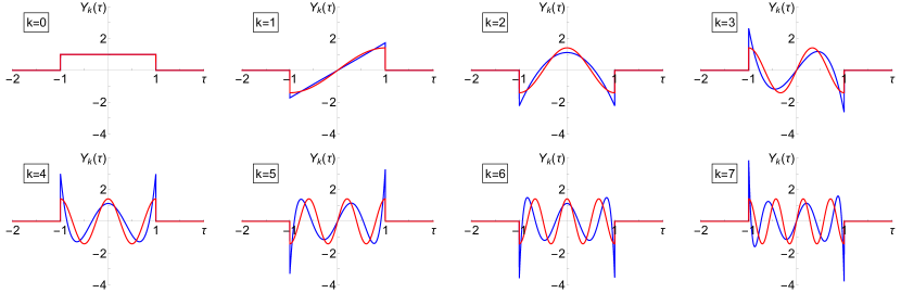
Figure 1: First eight SSC harmonics $Y_{k}(\tau)$ for a bunch in a square potential well (red) and $\text{HP}_{0}$ distribution (blue). The harmonics are presented in dimensionless units. Note that for both distributions $\rho(\tau)=1/2$.

Expansion over the SSC harmonics

$$\mathcal{Y}_{k}(\tau)=\sum_{i=0}^{\infty}\mathbf{C}^{(k)}_{i}Y_{i}(\tau)$$ (9)

leads to the eigenvalue problem $\mathbf{M}\cdot\mathbf{C}^{(k)}=\Delta q_{k}\mathbf{C}^{(k)}$ where

$$\mathbf{M}_{lm}=\nu_{l}\,\delta_{lm}+\kappa\,\widehat{\mathrm{W}}_{lm}$$ (10)

with matrix elements of the wake operator being

$$\widehat{\mathrm{W}}_{lm}=\int_{-\infty}^{\infty}\int_{\tau}^{\infty}W(\tau-\sigma)\,\rho(\tau)\,\rho(\sigma)\,Y_{l}(\tau)\,Y_{m}(\sigma)\,\mathrm{d}\,\sigma\,\mathrm{d}\,\tau.$$ (11)

Below, real and imaginary parts of the eigenvalues are denoted as

$$\Delta q_{k}=\Delta_{k}+i\,\Gamma_{k}.$$ (12)

As it was demonstrated by V. Balbekov Balbekov (2017b), the expansion over the SSC harmonics may have a poor convergence, so that the numerically obtained instability threshold is very sensitive to the accuracy of the matrix elements computation and the number of harmonics taken into account. In order to distinguish the illusory, pure numerical, threshold from the real one, two things are required: a large number of the basis harmonics and high accuracy of the computed matrix elements. To provide that, we considered two different distributions with constant line density, where the matrix elements can be computed analytically, thus minimizing numerical errors up to machine precision and justifying to include large number of modes into analysis.

II.1.1 Square potential well

Our first SSC model relates to a bunch in the square potential well (SSCSW, stays for Strong Space Charge, Square Well). In this case the distribution function is factorized

$$f_{\text{sw}}(\tau,\mathrm{v})=\frac{1}{2\,a}\text{H}\left[1-\frac{\tau^{2}}{a^{2}}\right]\mathrm{V}(\mathrm{v}).$$ (13)

Below we omit the Heaviside function, assuming that all bunch related functions are defined on its length, $|\tau|\leq a$. The average square of velocity is position-independent,

$$u_{\text{sw}}^{2}(\tau)\equiv b^{2}.$$ (14)

Then, the equation for the SSC harmonics can be written as

$$0=\nu\,Y_{k}^{\text{sw}}(\tau)+\frac{b^{2}}{Q_{\text{eff}}(0)}\frac{\mathrm{d}}{\mathrm{d}\tau}\left[\frac{\mathrm{d}}{\mathrm{d}\tau}\,Y_{k}^{\text{sw}}(\tau)\right].$$ (15)

With $\tau$ measured in units of $a$ and $\nu$ in units of $\pi^{2}b^{2}/[4\,a^{2}Q_{\text{eff}}(0)]$, it reduces to

$$\left\{\begin{array}[]{l}\displaystyle Y^{\prime\prime}(\tau)+\frac{\pi^{2}}{4}\,\nu\,Y(\tau)=0,\\[7.11317pt] Y^{\prime}(\pm 1)=0.\end{array}\right.$$ (16)

This S-L problem yields the eigenvalues as integers squared,

$$\nu_{k}^{\text{sw}}=\left\{k^{2}\,|\,k\in\mathbb{Z}\right\}=\left\{0,1,4,9,25,36,\ldots\right\}.$$ (17)

The set of eigenfunctions consists of the constant 0-th mode $Y^{\text{sw}}_{0}=1$ and a sequence of cosine and sine functions (see Fig. 1)

$$Y_{k}^{\text{sw}}(\tau)=\left\{\begin{array}[]{lll}\displaystyle\sqrt{2-\delta_{0k}}\,\cos\frac{\pi\,k\,\tau}{2},&&k\text{ is even},\\[7.11317pt] \displaystyle\sqrt{2}\,\sin\frac{\pi\,k\,\tau}{2},&&k\text{ is odd}.\end{array}\right.$$ (18)

Note that the functions are normalized according to the general SSC harmonics orthonormalization rule (3) with $\rho(\tau)=\frac{1}{2}$.

II.1.2 Hofmann-Pedersen distribution

Another SSC model, where matrix elements for some wakes can be analytically calculated, is a bunch with a constant line density inside a parabolic potential well. Following M. Blaskiewicz, this distribution was previously referred as a boxcar, but since all our models have a boxcar, or constant, line density, in order to avoid confusions, we refer to it as the $\text{HP}_{0}$ model, or zeroth Hofmann-Pedersen distribution. Its phase space density is

$$f_{\text{hp}}^{(0)}(\tau,\mathrm{v})=\frac{\text{H}\left[1-\frac{\tau^{2}}{a^{2}}-\frac{v^{2}}{b^{2}}\right]}{2\,\pi\,a\,b}\left(1-\frac{\tau^{2}}{a^{2}}-\frac{v^{2}}{b^{2}}\right)^{-1/2}.$$ (19)

Normalized line density and temperature function are computed as

$$\rho(\tau)=\frac{1}{2},\qquad\qquad u_{\text{hp}}^{2}(\tau)=\frac{b^{2}}{2}\left(1-\frac{\tau^{2}}{a^{2}}\right).$$ (20)

This notation assumes a generalized Hofmann-Pedersen distribution of $n$-th order,

$$f_{\text{hp}}^{(n)}\propto(1-\tau^{2}/a^{2}-v^{2}/b^{2})^{n-1/2},$$ (21)

so the conventional Hofmann-Pedersen distribution Hofmann and Pedersen (1979), with its parabolic line density, can be addressed as $f_{\text{hp}}^{(1)}$. In this paper, only zero-order case $\text{HP}_{0}$ is considered, so the subscript ₀ can be safely omitted.

The equation for SSC harmonics

$$\nu\,Y_{k}^{\text{hp}}(\tau)+\frac{b^{2}}{2\,Q_{\text{eff}}(0)}\frac{\mathrm{d}}{\mathrm{d}\tau}\left[\left(1-\frac{\tau^{2}}{a^{2}}\right)\frac{\mathrm{d}}{\mathrm{d}\tau}\,Y_{k}^{\text{hp}}(\tau)\right]=0$$

can be conveniently written in the normalized variables, when $\tau$ is measured in units of $a$ and $\nu$ in units of $b^{2}/[a^{2}Q_{\text{eff}}(0)]$,

$$\frac{\mathrm{d}}{\mathrm{d}\tau}\left[\left(1-\tau^{2}\right)\frac{\mathrm{d}}{\mathrm{d}\tau}\,Y_{k}^{\text{hp}}(\tau)\right]+2\,\nu\,Y_{k}^{\text{hp}}(\tau)=0.$$ (22)

Note that $\nu$ is measured in different units in SSCSW and SSCHP; this choice was made in order to have first eigenvalues $\nu_{1}=1$ for the both models.

For this distribution, the S-L problem doesn’t have solutions, which relates to the singularities in Eq. (22) at $\tau=\pm 1$. One way to overcome this problem is to add a small regularization term $\epsilon>0$,

$$Y^{\prime\prime}(\tau)-\frac{2\,\tau}{1+\epsilon-\tau^{2}}\,Y^{\prime}(\tau)+\frac{2\,\nu}{1+\epsilon-\tau^{2}}\,Y(\tau)=0,$$ (23)

thus removing the singularity within the same bunch length $[-1;1]$. With this regularization, the S-L solutions do exist, and, as $\epsilon\rightarrow 0$, the eigenvalues converge to the triangular numbers

$$\nu_{k}^{\text{hp}}=\left\{k\,(k+1)/2\,|\,k\in\mathbb{Z}\right\}=\left\{0,1,3,6,10,15,\ldots\right\}.$$ (24)

The eigenfunctions converge to ones proportional to the Legendre polynomials $P_{k}(\tau)$,

$$Y_{k}^{\text{hp}}=(-1)^{\left\lfloor{k/2}\right\rfloor}\sqrt{2\,k+1}\,P_{k}(\tau)$$ (25)

where the floor function $\left\lfloor n\right\rfloor$ is an integer part of $n$, and $(-1)^{\left\lfloor k/2\right\rfloor}$ factor guarantees that each even (odd) harmonic has cosine-like (sine-like) properties at the origin, see Eq. (26). These SSC harmonics are presented in Fig. 1.

Another way to find eigenvalues is to look for an even and odd functions with

$$\left\{\begin{array}[]{l}Y\phantom{{}^{\prime}}(0)=1,\\ Y^{\prime}(0)=0,\end{array}\right.\qquad\text{or}\qquad\left\{\begin{array}[]{l}Y\phantom{{}^{\prime}}(0)=0,\\ Y^{\prime}(0)=1,\end{array}\right.$$ (26)

respectively. When the small regularization term $\epsilon>0$, the derivatives $Y^{\prime}(\pm 1)$ vanish for the same triangular values, $\nu_{k}^{\text{hp}}$. With $\epsilon=0$, only the triangular eigenvalues $\nu=k(k+1)/2$ yield the solutions, remaining finite at the bunch edges $\tau=\pm 1$. Analytical expressions for the matrix elements $\widehat{\mathrm{W}}_{lm}$ are provided in Appendix A.

II.2 Airbag in a square well

In addition to SSC cases, we consider the airbag longitudinal distribution inside a square well, abbreviated as ABS (AirBag Square well) model,

$$f_{\mathrm{ABS}}(\tau,\mathrm{v})\propto\left[\delta(\mathrm{v}-\mathrm{v}_{0})+\delta(\mathrm{v}+\mathrm{v}_{0})\right]\text{H}\left[1-4\,\frac{\tau^{2}}{\tau_{\mathrm{b}}^{2}}\right],$$ (27)

suggested by M. Blaskiewicz Blaskiewicz (1998). For a wide class of wake functions, the bunch spectrum can be found for arbitrary space charge tune shift, without expansion over an infinite set of basis function, thus avoiding the related convergence problem.

It is convenient to take for this model the following convention $\tau\in[-\tau_{\mathrm{b}}/2;\tau_{\mathrm{b}}/2]$ for the position along the bunch, where all particles move with the same absolute value of the velocity, $\mathrm{d}\,\tau/\mathrm{d}\theta=\pm\mathrm{v}_{0}$. Transverse offsets in the two fluxes of particles $X_{\pm}(\theta,\tau)$ can be looked for as

$$X_{\pm}(\theta,\tau)=e^{-i\,(Q_{\beta}+\Delta Q_{k})\theta}x_{\pm}(\tau)$$ (28)

where$Q_{\beta}$ is the bare betatron tune and $\Delta Q_{k}$ is the tune shift to be found. Then, equations for the amplitudes along the bunch $x_{\pm}(\tau)$ are given by

$$\frac{\mathrm{d}\,x_{+}}{\mathrm{d}\tau} = \frac{i}{\mathrm{v}_{0}}\left[\left(\frac{\Delta Q_{\mathrm{sc}}}{2}+\Delta Q_{k}\right)x_{+}-\frac{\Delta Q_{\mathrm{sc}}}{2}\,x_{-}-F\right],\qquad$$ (29)

$$\frac{\mathrm{d}\,x_{-}}{\mathrm{d}\tau} = \frac{i}{\mathrm{v}_{0}}\left[\frac{\Delta Q_{\mathrm{sc}}}{2}\,x_{+}-\left(\frac{\Delta Q_{\mathrm{sc}}}{2}+\Delta Q_{k}\right)x_{-}+F\right],\qquad$$ (30)

with the boundary conditions

$$\begin{array}[]{c}x_{+}(\tau_{\mathrm{b}}/2)=x_{-}(\tau_{\mathrm{b}}/2),\\[5.69046pt] x_{+}(-\tau_{\mathrm{b}}/2)=x_{-}(-\tau_{\mathrm{b}}/2).\end{array}$$ (31)

The force is defined by a wake function

$$F(\tau)=\kappa\,\int_{\tau}^{\tau_{\mathrm{b}}/2}W(\tau-\sigma)\,\overline{x}(\sigma)\,\mathrm{d}\sigma$$ (32)

and satisfies an integro-differential equation:

$$\frac{\mathrm{d}\,F(\tau)}{\mathrm{d}\tau}=-\kappa\,W(0)\,\overline{x}(\tau)+\kappa\,\int_{\tau}^{\tau_{\mathrm{b}}/2}\frac{\partial}{\partial\tau}W(\tau-\sigma)\overline{x}(\sigma)\,\mathrm{d}\sigma$$ (33)

with $\overline{x}=(x_{+}+x_{-})/2$. For a wake function in the form

$$W(\tau)=-W_{0}\,\sum_{k=1}^{n}C_{k}\,e^{\alpha_{k}\,\tau}$$ (34)

the force is

$$F=\sum_{k=1}^{n}F_{k}=-\kappa\,W_{0}\sum_{k=1}^{n}C_{k}\int_{\tau}^{\tau_{\mathrm{b}}/2}e^{\alpha_{k}(\tau-\sigma)}\,\overline{x}(\sigma)\,\mathrm{d}\sigma,$$ (35)

and for every $k=1,\ldots,n$,

$$\frac{\mathrm{d}\,F_{k}(\tau)}{\mathrm{d}\tau}=\frac{\kappa\,W_{0}}{2}\,C_{k}(x_{+}+x_{-})+\alpha_{k}\,F_{k},$$ (36)

with $F_{k}(\tau_{\mathrm{b}}/2)=0$.

Measuring $\tau$ in units of $\tau_{\mathrm{b}}$ and defining

$$f(\tau)=F(\tau)/Q_{\text{s}}$$ (37)

where $Q_{\text{s}}=\pi\,\mathrm{v}_{0}/\tau_{\mathrm{b}}$ is the synchrotron tune, Eqs. (29,30) and (36) can be presented as a set of ordinary linear homogeneous differential equations,

$$\frac{\mathrm{d}\,\mathrm{U}}{\mathrm{d}\tau}=\mathrm{M}\,\mathrm{U},$$ (38)

with boundary conditions

$$f_{k}(1/2) = 0,$$ (39)

$$x_{+}(1/2) = x_{-}(1/2),$$ (40)

$$x_{+}(-1/2) = x_{-}(-1/2),$$ (41)

where $\mathrm{U}=(x_{+},x_{-},f_{1},f_{2},\ldots)$, and the matrix $\mathrm{M}$ is combined from the coefficients. To solve this set of equations, we suggest an algorithm different from one applied by M. Blaskiewicz.

The differential Eq. (38), first, can be transformed into a difference one,

$$\mathrm{U}_{n+1}-\mathrm{U}_{n}=\Delta\tau\,\mathrm{M}\,\mathrm{U}_{n}.$$ (42)

Choosing $n=2^{m}$ and $\Delta\tau=1/2^{m}$, for $\mathrm{U}_{n}\equiv\mathrm{U}(1/2)=(1,1,0,0,\ldots)$ one has

$$\mathrm{U}_{0}\equiv\mathrm{U}(-1/2)=\left(\frac{1}{2^{m}}\,\mathrm{M}+\mathrm{I}\right)^{-2^{m}}\,\mathrm{U}_{n}.$$ (43)

Those values of $\Delta Q_{k}$, with which the boundary condition at the tail of the bunch is satisfied, i.e.

$$x_{+}^{(0)}-x_{-}^{(0)}=0,$$ (44)

constitute the bunch spectrum; they can be found by a proper scan of the complex plane of $\Delta Q_{k}$. However, for the instability thresholds, it is sufficient to scan only real $\Delta Q_{k}$: the threshold can be detected as reduction of the number of these real modes by two.

This algorithm proves to be extremely time-efficient; the solution always converges with the number of intervals $1/\Delta\tau$, while the CPU time grows only logarithmically, $\propto\log_{2}(1/\Delta\tau)=m$.

For the no-wake case, the ABS spectrum is calculated as

$$\frac{\Delta Q_{k}}{Q_{\text{s}}}=-\frac{\Delta Q_{\mathrm{sc}}}{2\,Q_{\text{s}}}\pm\ \sqrt{\left(\frac{\Delta Q_{\mathrm{sc}}}{2\,Q_{\text{s}}}\right)^{2}+k^{2}},$$ (45)

for $k=\pm 1,\pm 2,\ldots$ and additional zeroth mode $\Delta Q_{0}=0$ which is not affected by the SC. When the SC becomes strong,

$$\Delta Q_{\mathrm{sc}}\gg 2\,k\,Q_{\text{s}}$$ (46)

the equidistant spectrum of integers (for $\Delta Q_{\mathrm{sc}}=0$) separates on positive part, quadratic with $k$: $\Delta Q_{k}\propto k^{2}$, and negative part, with $\Delta Q_{k}\approx-\Delta Q_{\mathrm{sc}}$ (see Fig. 2). In order to make a comparison with the SSC case, we use normalized tunes

$$\Delta q_{k}=\Delta Q_{k}/\Delta Q_{1},$$ (47)

so that the distance between the first and zeroth modes is equal to one for any value of the SC parameter, $Q_{\text{eff}}(0)/Q_{\text{s}}$, when there is no wake. When condition (46) is satisfied, ABS positive spectrum coincides with the SSCSW one:

$$\Delta Q_{k}=k^{2}Q_{\text{s}}^{2}/\Delta Q_{\mathrm{sc}},\qquad k=0,1,2,\ldots.;$$ (48)

for the SSCSW model, all the details of the longitudinal phase space density may play a role only by means of the average synchrotron frequency $Q_{\text{s}}$.

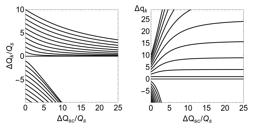
Figure 2: Eigenvalues (left) and normalized eigenvalues (right) for the ABS model as functions of the SC parameter for no-wake case, $k=-9,\ldots,10$.

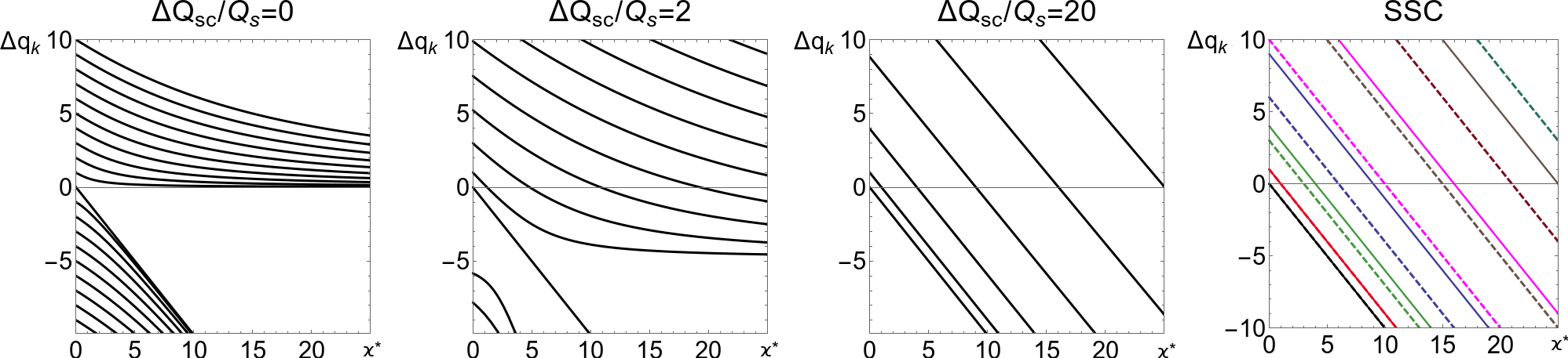
Figure 3: Normalized tune shifts for the ABS model and delta wake for different values of the SC parameter (first three plots). The last figure shows same values for the SSCSW (solid lines) and SSCHP (dashed lines) models.

Figure 4: Spectra for the ABS model and constant (top row) or exponential (bottom row) wakes. Different columns correspond to different values of the space charge parameter $\Delta Q_{\mathrm{sc}}/Q_{\text{s}}=0,2,20,200$. The TMCI thresholds are shown by black points.

III Negative wakes

Without wakes, all the modes are divided into two groups, with positive and negative tune shifts $\Delta Q_{k}$; at growing SC, the former tend to zero, while the latter tend to the SC tune shift. It is convenient to keep the same mode number when the wake, when introduced, tunes it up or down. Therefore, here-below a number of a particular mode for non-zero wake is defined as such of that zero-wake mode, which corresponds to the given mode when the wake amplitude continuously goes to zero. This mode number definition is unambiguous provided that the given mode never coupled with its neighbors at smaller wake amplitudes, which is sufficient for our purposes. Following that, we distinguish all the modes at any wake between positive and negative modes, or positive or negative parts of the spectrum, which is unambiguous provided that there is no coupling between the positive and negative modes, which is always the case below. The reader should not be confused by the fact that wakes may shift tunes of some positive modes to negative values; we still refer to such modes as positive.

In this section, constant-sign wakes are considered for the ABS, as well as for the SSC problems; as it follows from the Maxwell equations, this sign can only be negative Chao (1993). We limit ourselves here by delta-functional, exponential and resistive wall wakes. Sometimes, the tunes at a given wake and SC are convenient to present in units of the first eigenvalue at the same SC and zero wake. For that sake we will modify the intensity parameter $\kappa$ such that it will be measured in the units of

$$b^{2}/[Q_{\text{eff}}(0)\,a^{2}]\quad\text{and}\quad b^{2}/[2\,Q_{\text{eff}}(0)\,a^{2}],$$ (49)

for the SSCSW and the SSCHP models respectively. We hope that the factor of 2 difference here will not confuse the reader; it is dictated by our choice to have same formulas for the first eigenvalue for the two SSC cases at zero wake.

Dividing $\kappa$ by the first zero-wake eigenvalue at the given SC parameter, we define a normalized intensity parameter

$$\kappa^{*}=\kappa\Big{/}\left[-\frac{\Delta Q_{\mathrm{sc}}}{2\,Q_{\text{s}}}+\ \sqrt{\left(\frac{\Delta Q_{\mathrm{sc}}}{2\,Q_{\text{s}}}\right)^{2}+1}\right].$$ (50)

When $\kappa^{*}$ is used instead of $\kappa$, the positive part of the spectrum shows scale invariance for large values of $\Delta Q_{\mathrm{sc}}$, Eq. (46). In addition, in order to describe the instability we will introduce a parameter which is combining the intensity and the wake amplitude, respectively

$$\chi=\frac{\kappa\,W_{0}\tau_{\mathrm{b}}}{Q_{\text{s}}}\qquad\text{and}\qquad\chi^{*}=\frac{\kappa^{*}\,W_{0}\tau_{\mathrm{b}}}{Q_{\text{s}}}.$$ (51)

III.1 Delta wake

Our first negative-wake example is one of image charges, the delta wake,

$$W(\tau)=-W_{0}\,\delta(\tau).$$ (52)

In this case the airbag model allows analytical solution

$$\frac{\Delta Q_{k}}{Q_{\text{s}}}=-\frac{\Delta Q_{\mathrm{sc}}+\kappa\,W_{0}}{2\,Q_{\text{s}}}\pm\ \sqrt{\left(\frac{\Delta Q_{\mathrm{sc}}-\kappa\,W_{0}}{2\,Q_{\text{s}}}\right)^{2}+k^{2}},$$ (53)

for $k=\pm 1,\pm 2,\ldots$ and the zeroth mode $\Delta Q_{0}/Q_{\text{s}}=-\kappa\,W_{0}$. The system is stable for any values of wake amplitude and SC, Fig. 3 shows normalized tune shift as a function of wake amplitude for different values of SC.

For the SSC models, matrix elements are given by

$$\widehat{\mathrm{W}}_{lm}=-W_{0}\,\int_{\text{SB}}\rho^{2}(\tau)\,Y_{l}(\tau)\,Y_{m}(\tau)\,\mathrm{d}\tau=-W_{0}\,\frac{\delta_{lm}}{2},$$ (54)

yielding the eigenvalues

$$\Delta q_{k}=\nu_{k}+\kappa\,\widehat{\text{W}}_{kk}=\nu_{k}-\frac{\kappa\,W_{0}}{2}.$$ (55)

Beam stability for the delta wake is a consequence of that the system is Hamiltonian: the delta wake can be taken into account with a term proportional to a double sum $\Sigma_{lm}x_{l}x_{m}\delta(\tau_{l}-\tau_{m})$ in the total Hamiltonian, where $x_{l}$ and $x_{m}$ are offsets of individual particles and $\tau_{l}$, $\tau_{m}$ are their positions inside the bunch.

III.2 Exponential and constant wakes

As the next example, let’s consider exponential wakes

$$W(\tau)=-W_{0}\,e^{\alpha\,\tau},$$ (56)

including a constant wake, $\alpha=0$. Behavior of TMCI with these wakes was considered for ABS by M. Blaskiewicz and for HP and SW cases by V. Balbekov Balbekov (2016b, a, 2017a, 2017b). Here we summarize some of these results and make a comparison between models.

Fig. 4 shows normalized coherent tune shifts for constant and exponential ($\alpha=10$) wakes for the ABS model. As one can see, TMCI may occur only at the negative part of the spectrum and the thresholds monotonically increase with $\Delta Q_{\mathrm{sc}}$. Last two plots in each row look identical to each other, thus showing the SSC scaling. Behavior of the TMCI thresholds is summarized in Fig. 5 which we reproduce, albeit by another method, after M. Blaskiewicz Blaskiewicz (1998).

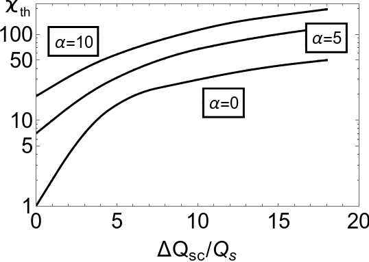
Figure 5: TMCI threshold as a function of space charge for the ABS model with the exponential wakes (reproduction of Ref. Blaskiewicz (1998)).

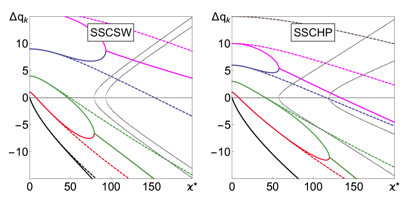
Figure 6: Real (shown in color) and imaginary (gray colors) parts of the spectra for SSCSW and SSCHP with a constant wake. Solid and dashed lines are obtained using 5 or 50 modes respectively. For sufficiently large number of modes and sufficiently good accuracy of the matrix element computations, TMCI vanishes.

Increase of the TMCI thresholds with the space charge, first demonstrated in Ref. Blaskiewicz (1998), soon after that was explained in Ref. Ng and Burov (1999): while the wake deflects down mostly the zeroth mode, and to a lesser extent does that for the mode $\Delta Q_{-1}$, the space charge does exactly the opposite, deflecting down the mode $\Delta Q_{-1}$ and keeping the tune of the mode $0$ untouched; thus, the mode crossing either happens at higher wakes, or does not happen at all. However, it was later speculated in Ref. Burov (2009) that the increase of the threshold with the space charge may be non-monotonic, that at sufficiently high SC tune shift, the TMCI threshold may start to go down. A reason for that speculation was derived from the unlimited reduction of the mode separation with the space charge; when the neighbor modes are closer and closer, it should take less and less to couple them. This speculation was apparently confirmed within the SSC approximation by computation of the TMCI threshold versus the SC tune shift with constant and resistive-wall wakes, where the non-monotonic behavior of the instability threshold was observed. However, those computations of Ref. Burov (2009) were made with not so high number of modes and with limited accuracy of the matrix element computation, so the formulated hypothesis remained open. This problem was recently addressed by V. Balbekov Balbekov (2017a, b). Specifically, it has been shown by him, that the TMCI threshold computed for the exponential wakes unlimitedly grows with the number of the basis functions taken into account. In other words, for such wakes at SSC case there is no TMCI at all, the instability may happen only with comparable SC and wake-driven tune shifts, as in Fig. 5. Here we confirm that with our results presented in Fig. 6. Solid lines show real and imaginary parts of the spectra for SSCSW and SSCHP cases for a constant wake and truncation at 5 harmonics. Dashed lines are the same spectra computed with 50 basis harmonics. As one can see, no instability observed in the considered range of $\kappa$ when number of harmonics is large enough. Note agreement between the ABS model (constant wake and large $\Delta Q_{\mathrm{sc}}$, top right plot in Fig. 4) and the SSCSW model (constant wake for large number of modes, left plot in Fig. 6).

Figure 7 shows growth of the instability thresholds with the number of harmonics in analysis for both models (SSCSW and SSCHP) with the constant wake. For all the cases, the thresholds monotonically increase with the mode truncation parameter, thus demonstrating that the beam is stable against TMCI.

When the instability threshold unlimitedly increases with SC, the TMCI is referred in this paper as vanishing.

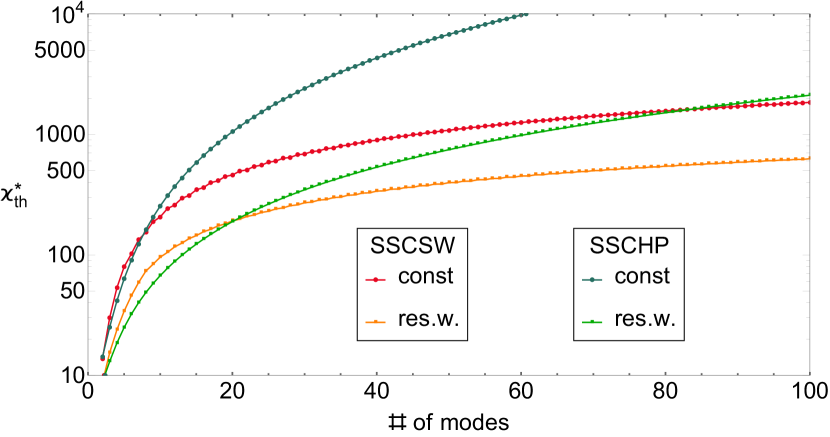
Figure 7: TMCI threshold as a function of number of modes for constant and resistive wall wakes (SSCSW and SSCHP models). The unlimited growth with the truncation parameter means that there is no TMCI.

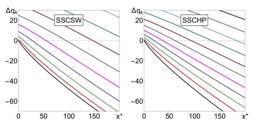
Figure 8: Spectra for SSCSW and SSCHP models with resistive wall wake, truncated at 50 modes. No TMCI.

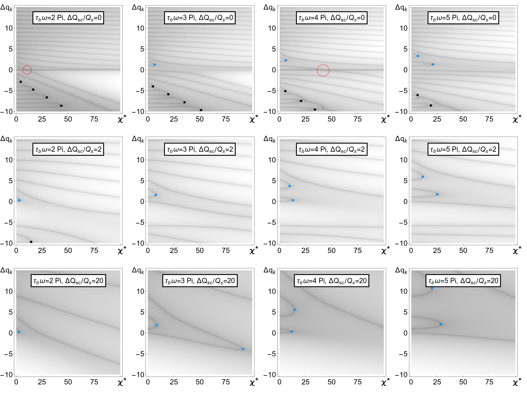
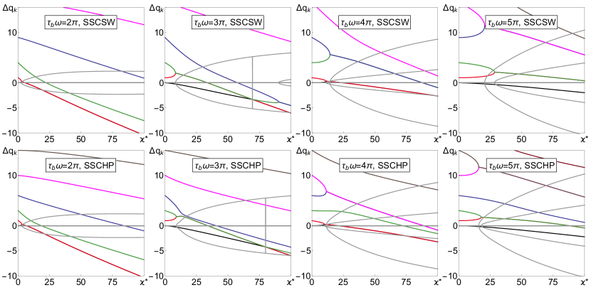
Figure 9: Bunch spectra for the cosine wake. The top three rows show the ABS spectra for various values of SC (0, 2, 20). The vanishing TMCI thresholds are shown with black points and non-vanishing with blue. The red dashed circles indicate mode crossing, when modes do not couple. The last two rows are for the SSCSW and SSCHP models; the real and imaginary parts of $\Delta q_{k}$ are shown in colors and in gray respectively. The columns correspond to different values of $\omega\,\tau_{\mathrm{b}}$ ($2\,\pi,3\,\pi,4\,\pi,5\,\pi$).

III.3 Resistive wall wake

The SSC models can also be considered with the resistive wall wake function

$$W(\tau)=-W_{0}/\sqrt{|\tau|}.$$ (57)

Similar to the exponential and constant wakes, the thresholds grow unlimitedly with the number of modes taken into account, as it can be seen in Fig. 7. Spectra for both SSCSW and SSCHP cases are shown in Fig 8.

IV Oscillating wakes

As shown above, the instability for negative wakes takes place only when wake and space charge tune shifts are comparable, i.e. the TMCI is of the vanishing type. At positive (non-physical) wakes, the instability threshold monotonically decreases with the space charge; the wake moves 0-th tune up, while the space charge deflects the tune of the above 1-st mode down, so SC helps the two modes to meet each other. However, the positive wake is non-physical, it is forbidden by Maxwell’s equations Chao (1993). What is possible, is a combination of positive and negative wakes, i.e. oscillatory wakes. It can be expected that, at least for some of them, the instability threshold decreases with the SC, similar to the positive wakes. In fact, this was already shown for the cosine wake in Ref. Burov (2009): contrary to negative, the cosine wake may deflect down a certain mode more than its lower neighbor, thus making modes crossing and possibly couple. Since SC reduces the mode separation, in this case, the instability threshold goes down with an increase of the SC tune shift.

In this section, we consider oscillating wakes of two types: cosine and sine with variable decay rates. All of them can be treated within the ABS model, as suggested in Ref. Blaskiewicz (1998). For comparison, results of the complimentary SSC approximation are also provided below.

IV.1 Cosine wake

For cosine wakes

$$W(\tau)=-W_{0}\cos(\omega\,\tau),$$ (58)

the normalized spectra for different values of the SC tune shift and the wake phase advance $\omega\,\tau_{\mathrm{b}}$ are shown in Fig. 9. It shows that the situation is more diverse here than for the negative wakes: in addition to instabilities in the negative part of the spectra (indicated with black points again), there is a mode coupling in the positive parts of the spectra (blue points) as well. Figure 10 summarizes the behavior of the lowest mode coupling thresholds for the modes with negative and positive indexes. While TMCIs in the negative part of the spectra vanish, as it was for the case of constant-sign wakes, TMCI thresholds in the positive part of the spectra are non-monotonic, as it was speculated in Ref. Burov (2009); being growing at sufficiently small SC parameters, the thresholds become inversely proportional to the SC tune shift at its higher values, i.e. TMCI does not vanish. On the bottom plot, which repeats the top one in normalized units, one can see the stabilization of the non-vanishing TMCI threshold when modes, which cause the instability, reach the SSC limit.

At high SC parameter, all the models give similar results, while the SSCSW model fully coincides with the ABS (compare third and fourth rows in Fig. 9). In contrast to the case of negative wakes, the threshold computed for the SSC quickly converges with the number of modes taken into account. Examples of convergence of $\kappa_{\mathrm{TMCI}}$ are presented in Fig. 11. At the same time, when the number of modes becomes too large (which is about 30 in our case), the SSCHP model shows a pure numerical instability: the threshold computations become unstable and its erratically computed value drops to 0.

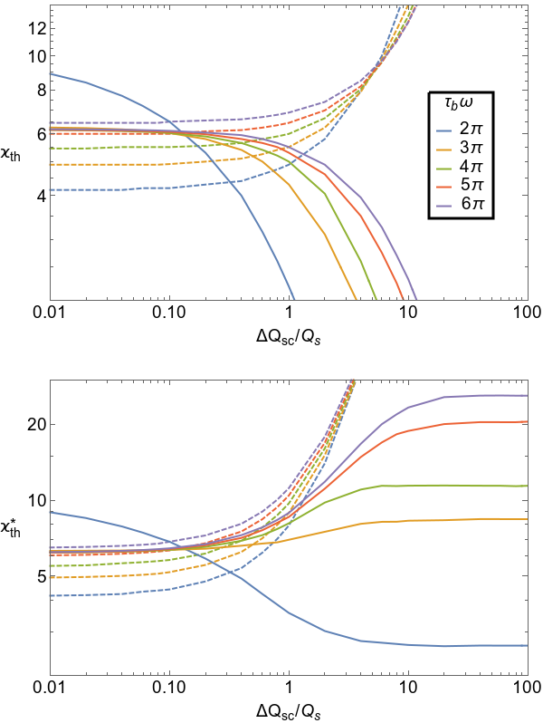
Figure 10: TMCI threshold as a function of space charge for the ABS model and a cosine wake. The dashed and solid lines correspond to the vanishing and non-vanishing TMCIs. The top figure shows thresholds in regular units. The bottom figure shows the same but using normalized eigenvalues: at every SC parameter, the eigenvalues are related to one of the first mode at zero wake.

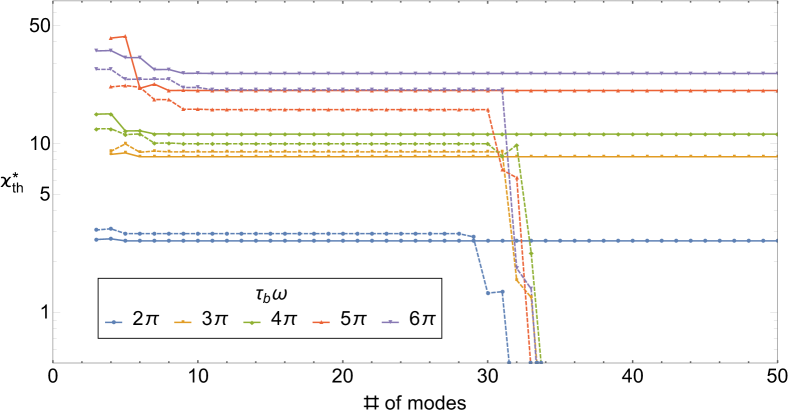
Figure 11: Instability threshold as a function of the number of modes taken into account at the SSC for the cosine wake. SSCSW and SSCHP models are shown using solid and dashed lines respectively. For the SSCHP model when the number of modes is $\approx 30$, there is a fast decrease of $\kappa_{\mathrm{TMCI}}$ reflecting the numerical error; such a numerical error was not observed for the SSCSW case up to 100 modes.

In order to summarize the behavior of $\kappa_{\mathrm{TMCI}}$ for SSC and the cosine wake, we considered it as a function of $\omega\,\tau_{\mathrm{b}}$ for both models, see Fig. 12. As expected, TMCI has a threshold with respect to $\omega\,\tau_{\mathrm{b}}\approx\pi$: for smaller values of the phase advance, the wake is effectively negative.

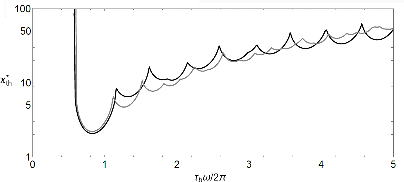
Figure 12: TMCI threshold as a function of wake phase advance $\omega\,\tau_{\mathrm{b}}$, for SSCSW (black) and SSCHP (gray) models with cosine wake. The vertical lines reflect an absolute threshold with respect to $\omega\,\tau_{\mathrm{b}}$.

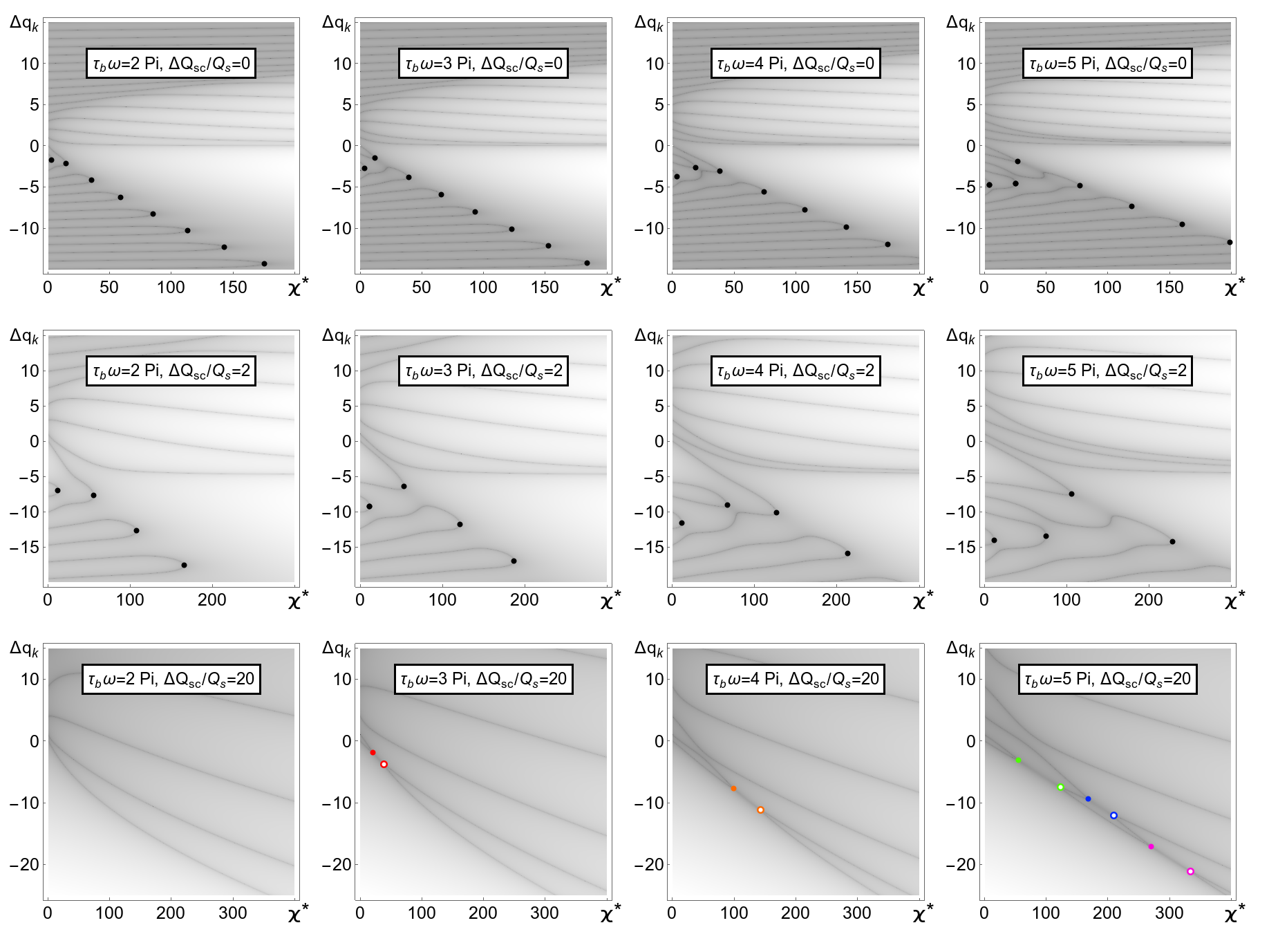
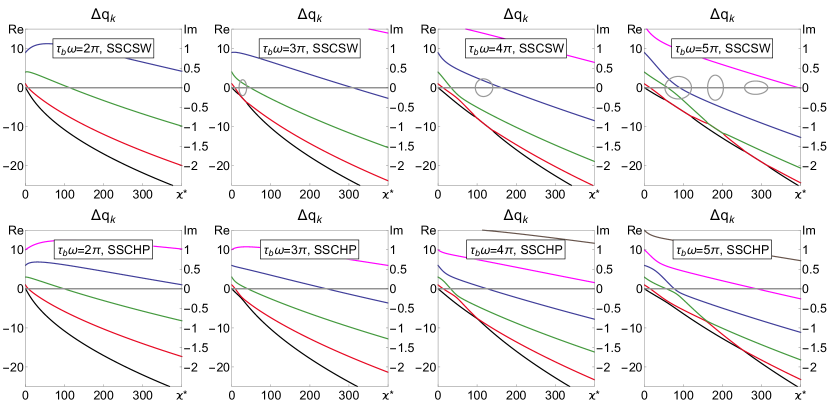
Figure 13: Bunch spectra for the sine wake. The top three rows show the ABS spectra for various values of SC (0, 2, 20). The vanishing TMCI thresholds are shown with black and non-vanishing using points in colors (subsequent decoupling for each TMCI is shown by the point of the same color with an annulus). The last two rows are for the SSCSW and SSCHP models; the real and imaginary parts of $\Delta q_{k}$ are shown in colors and in gray respectively (note the different scaling for $\Delta_{k}$ and $\Gamma_{k}$). The columns correspond to the different values of $\omega\,\tau_{\mathrm{b}}$ ($2\,\pi,3\,\pi,4\,\pi,5\,\pi$).

IV.2 Sine wake

The sine wake

$$W(\tau)=W_{0}\,\sin(\omega\,\tau),$$ (59)

is considered for the same three models, ABS, SSCSW and SSCHP; the resulting spectra are shown in Fig. 13. The behavior of the negative modes looks similar to the case of the cosine wake. In contrast, when the SC is zero, there is no instability for the positive modes, independently of the wake phase advance $\omega\tau_{\mathrm{b}}$. However, when the SC is increased, a cascade of mode couplings and decouplings appears. When $\omega\,\tau_{\mathrm{b}}=2\,\pi$, the threshold increases with the SC parameter, disappearing at the SSC case. The cases of $\omega\,\tau_{\mathrm{b}}=3\,\pi,4\,\pi$ show a single mode coupling followed by decoupling; the case $\omega\,\tau_{\mathrm{b}}=5\,\pi$ has a cascade of three couplings with subsequent decouplings. For wakes with even more oscillations per bunch, more complicated coupling-decoupling cascades were observed (not shown in the figure). Figure 14 summarizes the behavior of the lowest TMCI thresholds for both negative and positive modes. While all instabilities in the positive part of the spectrum decouple at higher values of $\kappa$, the values of these coupling and decoupling intensities go down inversely proportional to the SC parameter.

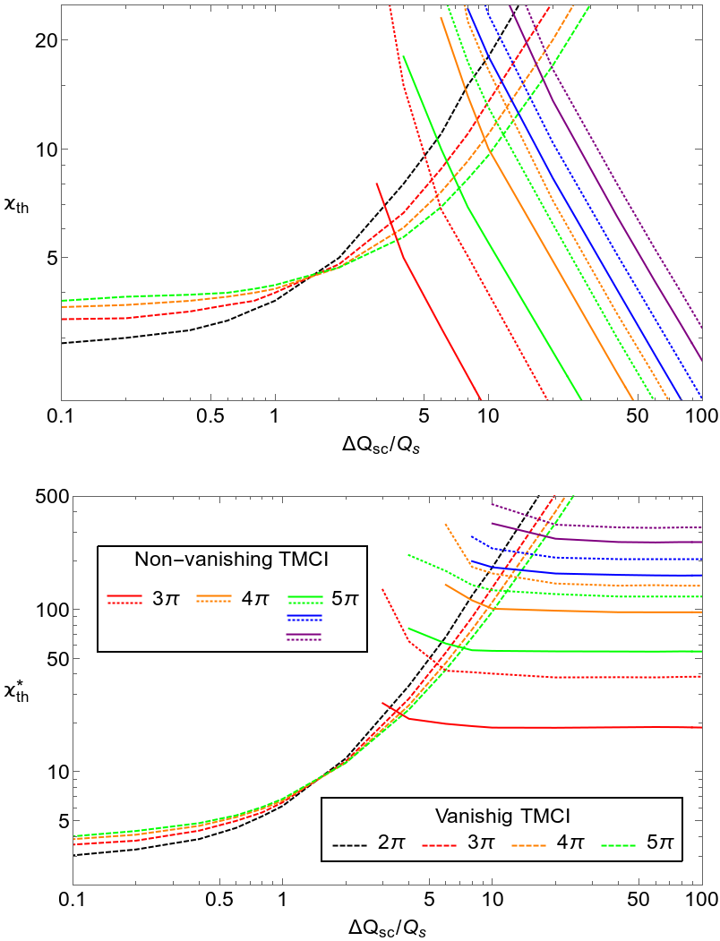
Figure 14: TMCI threshold in the usual (top) and normalized (bottom) units as a function of space charge for ABS model and sine wake. The dashed lines correspond to the vanishing TMCI in a negative part of the spectra. The solid and dotted lines represent mode couplings and decouplings in the positive part of the spectra.

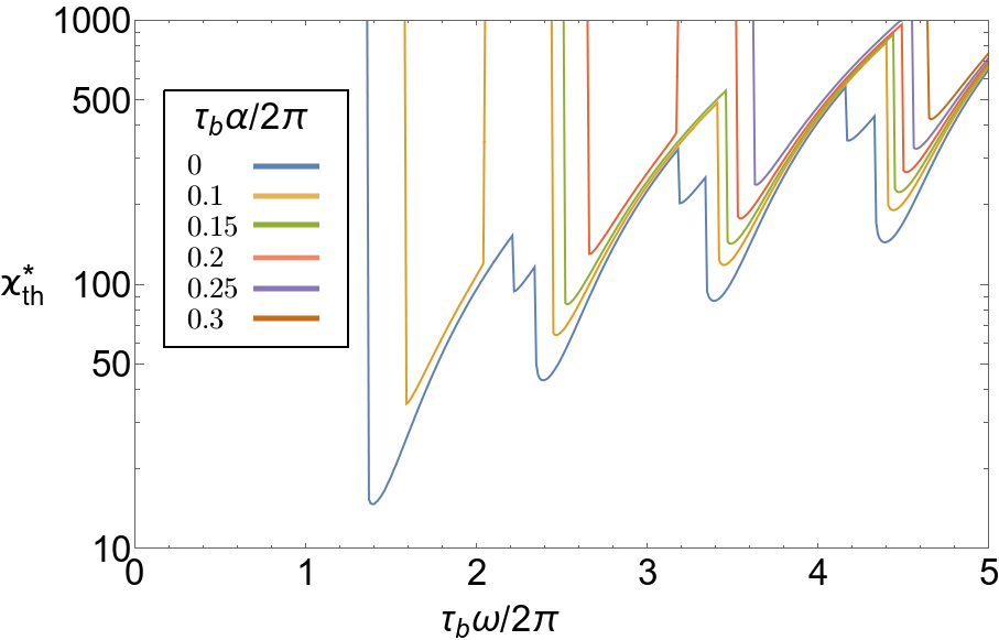
Figure 15: TMCI threshold for SSCSW model with broadband wake as a function of wake phase advance $\omega\,\tau_{\mathrm{b}}$. The different curves correspond to the different values of the wake decay rate, $\alpha\,\tau_{\mathrm{b}}$. The blue curve with $\alpha\,\tau_{\mathrm{b}}=0$ is for the sine wake. The vertical lines reflect an absolute threshold with respect to $\omega\,\tau_{\mathrm{b}}$.

Figure 13 shows that the SSCSW results agree with the ABS ones when the SC parameter is high enough (as they have to), while the SSCHP gives something unexpectedly different. Although the spectra of the SSCHP may look similar to both ABS and SSCSW models, they are different: the SSCHP modes never couple. Instead, they either simply cross or approach-divert with respect to each other without coupling. For this specific case there is an unknown reason forbidding the instability. This very unique property of the spectra is structurally unstable: the perturbation of $\nu_{k}^{\text{hp}}$ leads to the coupling-decoupling with instability, instead of mode crossing or approach-diverting.

The behavior of the non-vanishing TMCI as a function of $\omega\,\tau_{\mathrm{b}}$ for SSCSW is shown in Fig. 15. Similar to the cosine wake, the instability is impossible when $\omega\,\tau_{\mathrm{b}}\leq 2\,\pi$; otherwise, it happens and its threshold is a non-monotonic function of the wake phase advance $\omega\,\tau_{\mathrm{b}}$.

IV.3 Broadband wake

Finally, we consider how the spectrum for the sine wake is modified when a certain decay is added:

$$W=W_{0}\,\sin(\omega\,\tau)\,e^{\alpha\,\tau};$$ (60)

conventionally, this wake function is referred as broadband.

The result for the SSCSW model is shown in Fig. 15. There is no surprise that the instability threshold increases with $\alpha$ for fixed $\omega$. When a certain threshold with respect to the decay parameter $\alpha$ is reached, the instability vanishes: strong enough suppression of the oscillating part by the exponential effectively makes the wake negative. Thus, the TMCI does vanishes in certain zones of the wake decay and oscillation parameters $\alpha\tau_{\mathrm{b}}$ and $\omega\tau_{\mathrm{b}}$.

The ABS model confirms this result: for fixed $\omega$, when a threshold with respect to $\alpha$ is reached, instabilities in the positive part of the spectrum do not appear, even for large values of space charge. The only instabilities are in the negative part of the spectrum, vanishing with an increment of SC, as expected.

In the SSCHP model there is no instability as it was in the case of the sine wake; the mode crossing observed in the situation of the sine wake turns into an approach-divert behavior and the modes separate when $\alpha$ is increased.

V Summary

We questioned behavior of the transverse mode coupling thresholds as functions of space charge, wakes, potential wells and bunch distribution functions. Two different analytical models describing the bunch with constant line density had been used. The first one is the airbag model described in the article published by M. Blaskiewicz almost 20 years ago Blaskiewicz (1998). This model covers all values of space charge and yields an eigenvalue problem which is easily solved to machine precision for arbitrary combinations of the exponential and sinusoidal wakes. A complimentary model is given by the SSC theory Burov (2009, 2015); Balbekov (2009). In contrast to the ABS, it can be used only at sufficiently high SC tune shift, but it can be applied for any shape of the potential well and the bunch distribution function. As examples of the SSC models, we took an arbitrary bunch in a square well and the Hofmann-Pedersen distribution $f_{\text{hp}}^{(0)}$ for the parabolic potential well. They both yield analytical solutions, allowing to compute a large number of the wake matrix elements with extremely high accuracy, thus helping to distinguish pure numerical thresholds from the real ones. It has been demonstrated that in the SSC limit, Eq. (46), all the models give similar results, while the SSCSW fully coincides with the ABS, as expected. The SSCHP model demonstrates good quantitative agreement with the other two, except for a special case of a sine wake, where, for this distribution function, the modes may cross but never couple. In Section III we investigated negative wakes; our results agree with similar ones of M. Blaskiewicz and V. Balbekov: the TMCI thresholds tend to go linearly with the SC parameter, thus vanishing in the SSC case. the SC and

The situation is richer with possibilities for the oscillating wakes. First, an increase of TMCI threshold is non-monotonic here and, for sufficiently high SC parameter, TMCI threshold goes down inversely proportional to the SC tune shift, according to the hypothesis of Ref. Burov (2009): in addition to vanishing TMCIs in the negative part of the spectrum, there are non-vanishing TMCIs associated with couplings of the positive modes.

For the sine wake, three special features were seen. The first one is that when SC is zero, there is no instability for positive modes independent of the wake phase advance; but, when the SC is increased, a cascade of positive mode couplings and decouplings appear. These multiple couplings-decouplings for larger values of wake amplitude is the second major distinction. The last difference is that the HP model has a unique feature — there is no instability in SSC limit for the sine wake. It looks like an unknown theorem prohibits coupling for any value of wake amplitude for this case — one only observes the mode crossing or approach-divert behavior instead.

Based on our numerical results, we will conclude that the behavior of the TMCI thresholds with the SC parameter depends on the nature of wake function, roughly, on the number of its oscillations per bunch. When the wake function is negative, the TMCI is of the vanishing type: its threshold grows linearly with the SC parameter when the latter is high enough; the same is true for ”effectively” negative wakes, i.e. oscillating wakes with moderate phase advance, $\omega\,\tau_{\mathrm{b}}<\pi$, or the broadband wake with a sufficiently strong decay rate. For the oscillating wakes, the threshold dependence on the SC parameter should be expected as non-monotonic, going inversely proportional to the SC parameter when it is high enough.

Appendix A Matrix elements $\widehat{\mathrm{W}}_{lm}$ for SSC models

Wake function $W(\tau)$ and corresponding matrix elements $\widehat{\mathrm{W}}_{lm}$ for the SSCHP model are provided below in a Table 1. Calculation of matrix elements for SSCSW model boils down to standard integrals of two trigonometric and an exponential functions. They are easy to compute and the reader can find them using almost any symbolic computation program; matrix elements for sine and cosine wake functions should be calculated with care when $\omega\,\tau_{\mathrm{b}}=\pi\,n$ with $n=2,3,4,\ldots$ due to a resonance condition.

Table 1: Matrix elements $\widehat{\mathrm{W}}_{lm}$ for SSCHP model with negative (delta function, constant, exponential and resistive wall) and oscillating wakes (trigonometric and broadband impedance). $\widehat{\mathrm{W}}_{lm}$ for all oscillating wakes are expressed using matrix elements of exponential wake.

$W(\tau),\,\tau\leq 0$	$\widehat{\mathrm{W}}_{lm}$
Negative wakes
$-W_{0}\delta(\tau)$	$\displaystyle-\frac{W_{0}}{2}\,\delta_{l,m}$
$-W_{0}$	$\displaystyle-\frac{W_{0}}{2}\left[\delta_{lm,l-m}-(-1)^{\left\lfloor{l/2}\right\rfloor+\left\lfloor{m/2}\right\rfloor}\frac{\delta_{l,m+1}-\delta_{l,m-1}}{\sqrt{(2\,l+1)(2\,m+1)}}\right]$
$-W_{0}\exp(\alpha\,\tau)$	$\displaystyle-W_{0}\sum_{lm}^{ij}\frac{j!}{\alpha^{j+1}}\sum_{k=0}^{j}\frac{\alpha^{k}}{k!}\left\{\frac{1+(-1)^{i+k}}{i+k+1}-\frac{e^{-\alpha}}{(-\alpha)^{i+1}}\left[\Gamma(i+1,\alpha)-\Gamma(i+1,-\alpha)\right]\right\}$
$-W_{0}/\sqrt{|\tau|}$	$\displaystyle-W_{0}\sum_{lm}^{ij}\frac{2^{i+j+\frac{3}{2}}}{i+j+\frac{3}{2}}\,\sum_{k=0}^{j}\frac{(-1)^{i+k}}{j-k+\frac{1}{2}}\,\begin{bmatrix}j\\ k\end{bmatrix}\,_{2}F_{1}\left[-\left(i+j+\frac{3}{2}\right);-\left(i+k\right);-\left(i+j+\frac{1}{2}\right);\frac{1}{2}\right]$
Oscillating wakes
$-W_{0}\cos(\omega\,\tau)$	$\Re\left[\widehat{\mathrm{W}}_{lm}^{\mathrm{exp}}(i\,\omega)\right]$
$W_{0}\sin(\omega\,\tau)$	$-\Im\left[\widehat{\mathrm{W}}_{lm}^{\mathrm{exp}}(i\,\omega)\right]$
$W_{0}\sin(\omega\,\tau)\,\exp(\alpha\,\tau)$	$-\Im\left[\widehat{\mathrm{W}}_{lm}^{\mathrm{exp}}(\alpha+i\,\omega)\right]$

Appendix B Exponential and trigonometric wakes for ABS model

Matrix $\mathrm{M}$ for exponential, cosine and broadband impedance wakes is provided below in a Table 2.

Table 2: Matrix $\mathrm{M}$ for ABS model with exponential (or constant for $\alpha=0$), cosine and broadband impedance (or sine for $\alpha=0$) wake functions.

$W(\tau),\,\tau\leq 0$	$\mathrm{M}$
$-W_{0}\,e^{\alpha\,\tau}$	$\begin{bmatrix}i\,\pi\left(\frac{1}{2}\frac{\Delta Q_{\mathrm{sc}}}{Q_{\text{s}}}+\frac{\Delta Q_{k}}{Q_{\text{s}}}\right)&-i\,\pi\,\frac{1}{2}\frac{\Delta Q_{\mathrm{sc}}}{Q_{\text{s}}}&i\,\pi\\ i\,\pi\,\frac{1}{2}\frac{\Delta Q_{\mathrm{sc}}}{Q_{\text{s}}}&-i\,\pi\left(\frac{1}{2}\frac{\Delta Q_{\mathrm{sc}}}{Q_{\text{s}}}+\frac{\Delta Q_{k}}{Q_{\text{s}}}\right)&-i\,\pi\\ -\frac{1}{2}\frac{\kappa\,W_{0}\tau_{\mathrm{b}}}{Q_{\text{s}}}&-\frac{1}{2}\frac{\kappa\,W_{0}\tau_{\mathrm{b}}}{Q_{\text{s}}}&\alpha\,\tau_{\mathrm{b}}\\ \end{bmatrix}$
$-W_{0}\,\cos(\omega\,\tau)$	$\begin{bmatrix}i\,\pi\left(\frac{1}{2}\frac{\Delta Q_{\mathrm{sc}}}{Q_{\text{s}}}+\frac{\Delta Q_{k}}{Q_{\text{s}}}\right)&-i\,\pi\,\frac{1}{2}\frac{\Delta Q_{\mathrm{sc}}}{Q_{\text{s}}}&i\,\pi&i\,\pi\\ i\,\pi\,\frac{1}{2}\frac{\Delta Q_{\mathrm{sc}}}{Q_{\text{s}}}&-i\,\pi\left(\frac{1}{2}\frac{\Delta Q_{\mathrm{sc}}}{Q_{\text{s}}}+\frac{\Delta Q_{k}}{Q_{\text{s}}}\right)&-i\,\pi&-i\,\pi\\ -\frac{1}{4}\frac{\kappa\,W_{0}\tau_{\mathrm{b}}}{Q_{\text{s}}}&-\frac{1}{4}\frac{\kappa\,W_{0}\tau_{\mathrm{b}}}{Q_{\text{s}}}&i\,\omega\,\tau_{\mathrm{b}}&0\\ -\frac{1}{4}\frac{\kappa\,W_{0}\tau_{\mathrm{b}}}{Q_{\text{s}}}&-\frac{1}{4}\frac{\kappa\,W_{0}\tau_{\mathrm{b}}}{Q_{\text{s}}}&0&-i\,\omega\,\tau_{\mathrm{b}}\end{bmatrix}$
$W_{0}\,\sin(\omega\,\tau)\,e^{\alpha\,\tau}$	$\begin{bmatrix}i\,\pi\left(\frac{1}{2}\frac{\Delta Q_{\mathrm{sc}}}{Q_{\text{s}}}+\frac{\Delta Q_{k}}{Q_{\text{s}}}\right)&-i\,\pi\,\frac{1}{2}\frac{\Delta Q_{\mathrm{sc}}}{Q_{\text{s}}}&i\,\pi&i\,\pi\\ i\,\pi\,\frac{1}{2}\frac{\Delta Q_{\mathrm{sc}}}{Q_{\text{s}}}&-i\,\pi\left(\frac{1}{2}\frac{\Delta Q_{\mathrm{sc}}}{Q_{\text{s}}}+\frac{\Delta Q_{k}}{Q_{\text{s}}}\right)&-i\,\pi&-i\,\pi\\ -\frac{i}{4}\frac{\kappa\,W_{0}\tau_{\mathrm{b}}}{Q_{\text{s}}}&-\frac{i}{4}\frac{\kappa\,W_{0}\tau_{\mathrm{b}}}{Q_{\text{s}}}&(\alpha+i\,\omega)\,\tau_{\mathrm{b}}&0\\ \frac{i}{4}\frac{\kappa\,W_{0}\tau_{\mathrm{b}}}{Q_{\text{s}}}&\frac{i}{4}\frac{\kappa\,W_{0}\tau_{\mathrm{b}}}{Q_{\text{s}}}&0&(\alpha-i\,\omega)\,\tau_{\mathrm{b}}\end{bmatrix}$

References

- Chao (1993) A. W. Chao, Physics of collective beam instabilities in high energy accelerators (Wiley, 1993).
- Blaskiewicz (1998) M. Blaskiewicz, Physical Review Special Topics-Accelerators and Beams 1, 044201 (1998).
- Ng and Burov (1999) K. Ng and A. V. Burov, in AIP Conference Proceedings, Vol. 496 (AIP, 1999) pp. 49–63.
- Burov (2009) A. Burov, Physical Review Special Topics-Accelerators and Beams 12, 044202 (2009).
- Balbekov (2009) V. Balbekov, Physical Review Special Topics-Accelerators and Beams 12, 124402 (2009).
- Balbekov (2016a) V. Balbekov, arXiv preprint arXiv:1608.06243 (2016a).
- Balbekov (2016b) V. Balbekov, arXiv preprint arXiv:1607.06076 (2016b).
- Balbekov (2017a) V. Balbekov, Physical Review Accelerators and Beams 20, 034401 (2017a).
- Balbekov (2017b) V. Balbekov, arXiv preprint arXiv:1706.01982 (2017b).
- Chin et al. (2016) Y. H. Chin, A. W. Chao, and M. M. Blaskiewicz, Physical Review Accelerators and Beams 19, 014201 (2016).
- Hofmann and Pedersen (1979) A. Hofmann and F. Pedersen, IEEE transactions on nuclear science 26, 3526 (1979).
- Burov (2015) A. Burov, arXiv preprint arXiv:1505.07704 (2015).