Topological interpretation of Luttinger theorem

Abstract

Based solely on the analytical properties of the single-particle Green’s function of fermions at finite temperatures, we show that the generalized Luttinger theorem inherently possesses topological aspects. The topological interpretation of the generalized Luttinger theorem can be introduced because i) the Luttinger volume is represented as the winding number of the single-particle Green’s function and thus ii) the deviation of the theorem, expressed with a ratio between the interacting and noninteracting single-particle Green’s functions, is also represented as the winding number of this ratio. The formulation based on the winding number naturally leads to two types of the generalized Luttinger theorem. Exploring two examples of single-band translationally invariant interacting electrons, i.e., simple metal and Mott insulator, we show that the first type falls into the original statement for Fermi liquids given by Luttinger, where poles of the single-particle Green’s function appear at the chemical potential, while the second type corresponds to the extended one for non metallic cases with no Fermi surface such as insulators and superconductors generalized by Dzyaloshinskii, where zeros of the single-particle Green’s function appear at the chemical potential. This formulation also allows us to derive a sufficient condition for the validity of the Luttinger theorem of the first type by applying the Rouche’s theorem in complex analysis as an inequality. Moreover, we can rigorously prove in a non-perturbative manner, without assuming any detail of a microscopic Hamiltonian, that the generalized Luttinger theorem of both types is valid for generic interacting fermions as long as the particle-hole symmetry is preserved. Finally, we show that the winding number of the single-particle Green’s function can also be associated with the distribution function of quasiparticles, and therefore the number of quasiparticles is equal to the Luttinger volume. This implies that the fundamental hypothesis of the Landau’s Fermi-liquid theory, the number of fermions being equal to that of quasiparticles, is guaranteed if the Luttinger theorem is valid since the theorem states that the number of fermions is equal to the Luttinger volume. All these general statements are made possible because of the finding that the Luttinger volume is expressed as the winding number of the single-particle Green’s function at finite temperatures, for which the complex analysis can be readily exploited.

I Introduction

The Luttinger theorem states that the particle density of interacting fermions is equal to the volume in the momentum space enclosed by the Fermi surface Luttinger1960 . The theorem has been proved valid for normal Fermi liquids originally in perturbation expansion of the interacting single-particle Green’s function in 60’s Luttinger1960 ; Luttinger-Ward1960 and later in a non-perturbative way Oshikawa2000 . In the Green’s function language, the Luttinger volume is bounded by the surface, named Luttinger surface, in the momentum ($\mathbf{k}$) space on which the single-particle Green’s function $G(\mathbf{k},\omega=0)$ at zero frequency ($\omega$), i.e., at the chemical potential, changes its sign AGD . The fact that the single-particle Green’s function changes its sign in going through either poles or zeros AGD ; Dzyaloshinskii2003 allows Luttinger theorem to be extended even to insulating states Dzyaloshinskii2003 ; Essler2002 of interacting fermions, including multi-orbital systems Rosch2007 and non-translational-invariant systems Ortloff2007 . The extended versions of the Luttinger theorem are called the generalized Luttinger theorem, stating that the particle density of interacting fermions is equal to the Luttinger volume. The Luttinger theorem has also been shown valid for the Tomonaga-Luttinger liquid in one spatial dimension Yamanaka1997 .

Although the generalization of the Luttinger theorem has significant advantages, e.g., being able to treat metal and insulator on an equal footing Stanescu2006 ; Sakai2009 ; Imada2011 ; Eder2011 ; Stanescu2007 , its validity has been proved only for limited systems. For example, the validity of the generalized Luttinger theorem has been proved for a particle-hole symmetric single-band Hubbard model on the square lattice Stanescu2007 ; Phillips2012 . The proof is based on the moment expansion of the single-particle Green’s function, which involves the commutation relations of the Hamiltonian and electron creation/annihilation operators. Therefore, the proof depends on the microscopic Hamiltonian and thus it is difficult to generalize to other systems.

In this paper, we show that the Luttinger volume at zero temperature is expressed as the winding number of the determinant of the single-particle Green’s function. Therefore, the winding number of a ratio between the determinants of the interacting and noninteracting single-particle Green’s functions provides the topological interpretation of the generalized Luttinger theorem. We prove rigorously that the generalized Luttinger theorem is valid for generic interacting fermions as long as the particle-hole symmetry is preserved. The formulation based on the winding number of the single-particle Green’s function also allows us to naturally classify the condition for the validity of generalized Luttinger theorem into two types, depending on whether poles or zeros of the single-particle Green’s function exist at the chemical potential. The first type (type I) corresponds to the original statement for Fermi liquids given by Luttinger Luttinger1960 , whereas the second type (type II) corresponds to the extended one for single-particle gapful systems given by Dzyaloshinskii Dzyaloshinskii2003 . Moreover, a sufficient condition for the validity of the Luttinger theorem of type I can be derived from the topological interpretation of the theorem. Associating the winding number of the single-particle Green’s function with the distribution function of quasiparticles, we can show that the number of quasiparticle is equal to the Luttinger volume. These general results are based solely on analytical properties of the single-particle Green’s function at finite temperatures, for which the complex analysis can be exploited unambiguously, without any detail of a microscopic Hamiltonian, and can be applied in any spatial dimension to metallic and insulating states, independently of the strength of interactions. Several specific examples of interacting electrons are also provided to demonstrate these results.

The rest of the paper is organized as follows. Section II introduces the notation used in this paper and summarizes analytical aspects of the single-particle Green’s function at finite temperatures which are essential for the analysis in the following sections. Giving the definition of the Luttinger volume in Sec. III.1, we show in Sec. III.2 that the Luttinger volume is represented as the winding number of the determinant of the single-particle Green’s function in the zero-temperature limit. In Sec. III.3, the topological interpretation of the generalized Luttinger theorem is provided and the condition for the validity of the generalized Luttinger theorem is classified into two types (type I and type II). A sufficient condition for the validity of the generalized Luttinger theorem of type I is also derived. In Sec. III.4, the generalized Luttinger theorem is proved valid for generic interacting fermions as long as the particle-hole symmetry is preserved. To give specific examples for the generalized Luttinger theorem of types I and II, we examine a simple metal in Sec. IV.2 and a one-dimensional Mott insulator using the cluster perturbation theory (CPT) Senechal2000 ; Senechal2012 in Sec. IV.3, respectively. Finally, several remarks on the topological interpretation of the generalized Luttinger theorem are provided in Sec. V before summarizing the paper in Sec. VI. Additional discussions on the Luttinger-Ward functional and the quasiparticle distribution function at finite temperatures are given in Appendices A and C, respectively. The single-band Hubbard model on the honeycomb lattice is analyzed in Appendix B.

II Single-particle Green’s function

In this section, we shall derive useful analytical properties of the single-particle Green’s function at finite temperatures. As shown in Sec. III, the finite-temperature formulation introduced here significantly simplifies the analysis without encountering any ambiguity in treating the singularities of the single-particle Green’s function at the chemical potential, which is often overlooked in the zero-temperature formulation.

II.1 Notation

First, we introduce the notation for the single-particle Green’s function used here. We set $\hbar=k_{\rm B}=1$ and refer to $z$ ($\omega$) as complex (real) frequency. Following the notation in Ref. Aichhorn2006 , the Lehmann representation FW of the single-particle Green’s function at temperature $T$ is

$$G_{\alpha\beta}(z)=\sum_{m=1}^{N_{\rm ex}}\frac{Q_{\alpha m}Q_{\beta m}^{*}}{z-\omega_{m}}$$ (1)

with

$$Q_{\alpha m}=\sqrt{\mathrm{e}^{(\Omega-E_{r})/T}+\mathrm{e}^{(\Omega-E_{s})/T}}\langle r|c_{\alpha}|s\rangle$$ (2)

and $\omega_{m}=E_{s}-E_{r}$, where $m=(r,s)=1,2,\cdots,N_{\rm ex}$ represents all possible pairs of eigenstates $|r\rangle$ and $|s\rangle$ of Hamiltonian ${H}$ with their eigenvalues $E_{r}$ and $E_{s}$, respectively note2 . We adopt the convention that the chemical potential term is included in $H$ and therefore $z=0$ in $G_{\alpha\beta}(z)$ corresponds to the chemical potential. $\Omega=-T\ln\sum_{r}\mathrm{e}^{-E_{r}/T}$ is the grand potential and $c_{\alpha}$ is a fermion-annihilation operator with single-particle state $\alpha\,(=1,2,\cdots,L_{\rm s})$. For example, $\alpha$ can be a set of spin $\sigma$, momentum $\mathbf{k}$, and orbital $\xi$ indices [$\alpha\equiv(\sigma,\mathbf{k},\xi)$], or simply a site index $i$ ($\alpha\equiv i$). The Green’s function $G_{\alpha\beta}(z)$ is analytical in the complex plane except for the excitation energies at $\omega_{m}$ and thus poles of $G_{\alpha\beta}(z)$ appear only on the real-frequency axis.

The Green’s function is now written in an $L_{\rm s}\times L_{\rm s}$ matrix form

$$\boldsymbol{G}(z)=\boldsymbol{Q}\boldsymbol{g}(z)\boldsymbol{Q}^{\dagger},$$ (3)

where $\boldsymbol{Q}=\left[Q_{\alpha m}\right]$ is an $L_{\rm s}\times N_{\rm ex}$ rectangular matrix and

$$\boldsymbol{g}(z)={\rm diag}\left[1/(z-\omega_{1}),\cdots,1/(z-\omega_{N_{\rm ex}})\right]$$ (4)

is an $N_{\rm ex}\times N_{\rm ex}$ diagonal matrix with $\omega_{1}\leqslant\omega_{2}\leqslant\cdots\leqslant\omega_{N_{\rm ex}}$. The anti-commutation relation of the fermionic operators $\{c_{\alpha}^{\dagger},c_{\beta}\}=\delta_{\alpha\beta}$ guarantees the spectral weight sum rule, which is now written as $\sum_{m=1}^{N_{\rm ex}}Q_{\alpha m}Q_{\beta m}^{*}=\delta_{\alpha\beta}$ or equivalently

$$\boldsymbol{QQ}^{{\dagger}}=\boldsymbol{I}.$$ (5)

It should be noted that in general $\boldsymbol{Q}$ is not a unitary matrix, i.e., $\boldsymbol{QQ}^{\dagger}_{(L_{\rm s}\times L_{\rm s})}\not=\boldsymbol{Q}^{\dagger}\boldsymbol{Q}_{(N_{\rm ex}\times N_{\rm ex})}$, where the subscripts denote the size of the resulting matrices.

II.2 Diagonal elements of single-particle Green’s function

Next, we consider analytical properties of the diagonal element of the single-particle Green’s function $G_{\alpha\alpha}(z)$ Luttinger1961 ; Eder2014 ; Seki2016_2 ; Karlsson2016 because the particle number is evaluated through the trace of the single-particle Green’s function. It is apparent from Eq. (1) that the imaginary part of $G_{\alpha\alpha}(z)$, ${\rm Im}G_{\alpha\alpha}(z)$, is always finite when frequency $z$ is away from the real axis. Therefore, zeros of $G_{\alpha\alpha}(z)$ must lie on the real-frequency axis. The fact that the single-particle Green’s function is a rational function with respect to $z$ and $G_{\alpha\alpha}(z)\sim 1/z$ for large $|z|$ [see Eqs. (1) and (5)] ensures that the diagonal element of the single-particle Green’s function is in the following form:

$$G_{\alpha\alpha}(z)=\frac{\prod_{l=1}^{Z_{\alpha\alpha}}\left(z-\zeta_{l}^{(\alpha)}\right)}{\prod_{m=1}^{P_{\alpha\alpha}}\left(z-\omega_{m}^{(\alpha)}\right)}$$ (6)

with

$$P_{\alpha\alpha}-Z_{\alpha\alpha}=1,$$ (7)

where $\zeta_{l}^{(\alpha)}$ is a real frequency (with $\zeta_{1}^{(\alpha)}<\zeta_{2}^{(\alpha)}<\cdots<\zeta_{Z_{\alpha\alpha}}^{(\alpha)}$) at which $G_{\alpha\alpha}(\zeta_{l}^{(\alpha)})=0$, $\omega_{m}^{(\alpha)}\in\{\omega_{1},\omega_{2},\cdots,\omega_{N_{\rm ex}}\}$ with $\omega_{1}^{(\alpha)}<\omega_{2}^{(\alpha)}<\cdots<\omega_{P_{\alpha\alpha}}^{(\alpha)}$, and $Z_{\alpha\alpha}$ ($P_{\alpha\alpha}$) is the number of zeros (poles) of $G_{\alpha\alpha}(z)$ note . Here, $P_{\alpha\alpha}$ is counted only when the corresponding spectral weight is non-zero, i.e., $|Q_{\alpha m}|>0$. Thus, $P_{\alpha\alpha}$ can be smaller than $N_{\rm ex}$.

Typical frequency dependence of $G_{\alpha\alpha}(\omega)$ is shown in Fig. 1. The analytical properties of $G_{\alpha\alpha}(\omega)$ is understood as follows. Since

$$\boldsymbol{G}(z)^{\dagger}=\boldsymbol{Qg}(z)^{\dagger}\boldsymbol{Q}^{\dagger}=\boldsymbol{G}(z^{*}),$$ (8)

$\boldsymbol{G}(\omega)$ is Hermitian and thus $G_{\alpha\alpha}(\omega)$ is real for real frequency $\omega$. In the vicinity of a pole at $\omega_{m}^{(\alpha)}$, $G_{\alpha\alpha}(\omega)$ is positive (negative) on the right (left) side of $\omega_{m}^{(\alpha)}$ because

$$G_{\alpha\alpha}(\omega\simeq\omega_{m}^{(\alpha)})\simeq\frac{|Q_{\alpha m}|^{2}}{\omega-\omega_{m}^{(\alpha)}}$$ (9)

with the positive spectral weight, i.e., $|Q_{\alpha m}|^{2}>0$. On the other hand, its derivative

$$\frac{\partial G_{\alpha\alpha}(\omega)}{\partial\omega}=-\sum_{m=1}^{P_{\alpha\alpha}}\frac{|Q_{\alpha m}|^{2}}{(\omega-\omega_{m}^{(\alpha)})^{2}}$$ (10)

is always negative for $\omega\not=\omega_{m}^{(\alpha)}$, indicating that $G_{\alpha\alpha}(\omega)$ is a decreasing function of $\omega\,(\not=\omega_{m}^{(\alpha)})$. This immediately concludes that there must exist only a single frequency at which $G_{\alpha\alpha}(\omega)=0$ between two distinct successive real frequencies where $G_{\alpha\alpha}(\omega)$ exhibits poles, i.e.,

$$\omega_{1}^{(\alpha)}<\zeta_{1}^{(\alpha)}<\omega_{2}^{(\alpha)}<\cdots<\zeta_{Z_{\alpha\alpha}}^{(\alpha)}<\omega_{P_{\alpha\alpha}}^{(\alpha)},$$ (11)

with

$$\left\{\begin{array}[]{l}G_{\alpha\alpha}(\omega)>0,\ \ {\rm for}\,\,\omega_{m}^{(\alpha)}<\omega<\zeta_{m}^{(\alpha)}\\ G_{\alpha\alpha}(\omega)=0,\ \ {\rm for}\,\,\omega=\zeta_{m}^{(\alpha)}\\ G_{\alpha\alpha}(\omega)<0,\ \ {\rm for}\,\,\zeta_{m}^{(\alpha)}<\omega<\omega_{m+1}^{(\alpha)}\end{array}\right.,$$ (15)

as shown in Fig. 1.

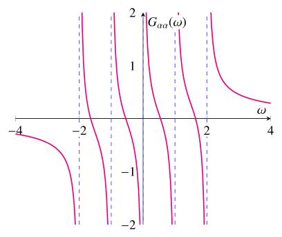
Figure 1: Schematic figure of the diagonal element of the single-particle Green’s function $G_{\alpha\alpha}(\omega)=\sum_{m}|Q_{\alpha m}|^{2}/(\omega-\omega_{m}^{(\alpha)})$ (thick solid lines) on the real-frequency axis $\omega$. This toy Green’s function $G_{\alpha\alpha}(\omega)$ has five poles at $\omega_{m}^{(\alpha)}=-2,-1,0,1,$ and $2$ (indicated by dashed vertical lines) with spectral weight $|Q_{\alpha m}|^{2}=1/5$ for $m=1,2,\cdots,5$.

II.3 Determinant of single-particle Green’s function

Let us now examine analytical properties of the determinant of the single-particle Green’s function, already analyzed to a certain extent in Refs. Dzyaloshinskii2003 , Karlsson2016 and Eder2008 . Here, we shall show that the determinant of the single-particle Green’s function can be expressed as a simple rational polynomial function as in Eq. (26) with the numbers of zeros and poles satisfying Eq. (29) (see also Appendix A of Ref. Seki2016_2 ).

From the Cauchy-Binet theorem, the determinant of the single-particle Green’s function

$$\det\boldsymbol{G}(z)=\det\left[\boldsymbol{Qg}(z)\boldsymbol{Q}^{\dagger}\right]$$ (16)

is identically zero if $N_{\rm ex}<L_{\rm s}$. However, generally $N_{\rm ex}\geq L_{\rm s}$ and thus we can safely assume that $\det\boldsymbol{G}(z)$ is not identically zero. From Eqs. (4) and (5), the asymptotic behavior of the determinant for large $|z|$ is $\det\boldsymbol{G}(z)\sim(1/z)^{L_{\rm s}}.$ This already suggests that $\det\boldsymbol{G}(z)$ has a form shown in Eqs. (26) and (29). In the following, we shall show that zeros of $\det\boldsymbol{G}(z)$ are all on the real-frequency axis.

Let us first triangularize $\boldsymbol{G}(z)$ by a unitary transformation (Schur decomposition),

$$\boldsymbol{R}(z)=\boldsymbol{U}(z)\boldsymbol{G}(z)\boldsymbol{U}(z)^{\dagger},$$ (17)

where $\boldsymbol{R}(z)$ is an upper triangle matrix and $\boldsymbol{U}(z)$ is a unitary matrix. From Eq. (3), $\boldsymbol{R}(z)$ can be written as

$$\boldsymbol{R}(z)=\tilde{\boldsymbol{Q}}(z)\boldsymbol{g}(z)\tilde{\boldsymbol{Q}}(z)^{\dagger},$$ (18)

where $\tilde{\boldsymbol{Q}}(z)=\boldsymbol{U}(z)\boldsymbol{Q}$ is an $L_{\rm s}\times N_{\rm ex}$ matrix with its matrix element

$$\tilde{Q}_{\alpha m}(z)=\sqrt{\mathrm{e}^{(\Omega-E_{r})/T}+\mathrm{e}^{(\Omega-E_{s})/T}}\langle r|\tilde{c}_{\alpha}(z)|s\rangle$$ (19)

and $\tilde{c}_{\alpha}(z)=\sum_{\beta=1}^{L_{\rm s}}U_{\alpha\beta}(z)c_{\beta}.$ It is apparent from Eq. (5) and the unitarity of $\boldsymbol{U}(z)$ that $\tilde{\boldsymbol{Q}}(z)$ fulfills the sum rule

$$\tilde{\boldsymbol{Q}}(z)\tilde{\boldsymbol{Q}}(z)^{\dagger}=\boldsymbol{I}$$ (20)

as $\{\tilde{c}_{\alpha}^{\dagger}(z),\tilde{c}_{\beta}(z)\}=\delta_{\alpha\beta}$.

The diagonal element of $\boldsymbol{R}(z)$ is now given as

$$R_{\alpha\alpha}(z)=\sum_{m=1}^{N_{\rm ex}}\frac{|\tilde{Q}_{\alpha m}(z)|^{2}}{z-\omega_{m}}.$$ (21)

Since the sum rule $\sum_{m=1}^{N_{\rm ex}}|\tilde{Q}_{\alpha m}(z)|^{2}=1$ must hold for arbitrary $z$, $\tilde{Q}_{\alpha m}(z)$ is bounded in the entire complex $z$ plane, and thus it must be constant, i.e.,

$$\tilde{Q}_{\alpha m}(z)=\tilde{Q}_{\alpha m},$$ (22)

known as Liouville’s theorem Ahlfors . Therefore, $R_{\alpha\alpha}(z)$ has the same analytical properties as $G_{\alpha\alpha}(z)$ and it is written as

$$R_{\alpha\alpha}(z)=\frac{\prod_{l=1}^{\tilde{Z}_{\alpha\alpha}}\left(z-\tilde{\zeta}_{l}^{(\alpha)}\right)}{\prod_{m=1}^{\tilde{P}_{\alpha\alpha}}\left(z-\tilde{\omega}_{m}^{(\alpha)}\right)}$$ (23)

with

$$\tilde{P}_{\alpha\alpha}-\tilde{Z}_{\alpha\alpha}=1,$$ (24)

where $\tilde{\zeta}_{z}^{(\alpha)}$($\tilde{\zeta}_{1}^{(\alpha)}<\tilde{\zeta}_{2}^{(\alpha)}<\cdots<\tilde{\zeta}_{Z_{\alpha\alpha}}^{(\alpha)}$) is a real frequency at which $R_{\alpha\alpha}(\tilde{\zeta}_{z}^{(\alpha)})=0$, and $\tilde{\omega}_{m}^{(\alpha)}\in\{\omega_{1},\omega_{2},\cdots,\omega_{N_{\rm ex}}\}$ with $\tilde{\omega}_{1}^{(\alpha)}<\tilde{\omega}_{2}^{(\alpha)}<\cdots<\tilde{\omega}_{\tilde{P}_{\alpha\alpha}}^{(\alpha)}$. $\tilde{Z}_{\alpha\alpha}$ ($\tilde{P}_{\alpha\alpha}$) is the number of zeros (poles) of $R_{\alpha\alpha}(z)$ note and $\tilde{P}_{\alpha\alpha}$ is counted only when the corresponding spectral weight is non-zero, i.e., $|\tilde{Q}_{\alpha m}|>0$. Similarly to Eq. (11), we can also show that

$$\tilde{\omega}_{1}^{(\alpha)}<\tilde{\zeta}_{1}^{(\alpha)}<\tilde{\omega}_{2}^{(\alpha)}<\tilde{\zeta}_{2}^{(\alpha)}<\cdots<\tilde{\zeta}_{Z_{\alpha\alpha}}^{(\alpha)}<\tilde{\omega}_{P_{\alpha\alpha}}^{(\alpha)}.$$ (25)

Since $\det\boldsymbol{G}(z)=\det\boldsymbol{R}(z)$, $\det\boldsymbol{G}(z)$ is now readily evaluated as

$$\det\boldsymbol{G}(z) = \prod_{\alpha=1}^{L_{\rm s}}\left[\frac{\prod_{l^{\prime}=1}^{\tilde{Z}_{\alpha\alpha}}\left(z-\tilde{\zeta}_{l^{\prime}}^{(\alpha)}\right)}{\prod_{m^{\prime}=1}^{\tilde{P}_{\alpha\alpha}}\left(z-\tilde{\omega}_{m^{\prime}}^{(\alpha)}\right)}\right]$$ (26)

$$= \frac{\prod_{l=1}^{Z_{\det}}\left(z-\tilde{\zeta}_{l}\right)}{\prod_{m=1}^{P_{\det}}\left(z-\tilde{\omega}_{m}\right)}$$

with

$$\tilde{\zeta}_{l}\in\{\tilde{\zeta}_{l^{\prime}}^{(\alpha)}|\alpha=1,2,\dots,L_{\rm s};\,l^{\prime}=1,2,\dots,\tilde{Z}_{\alpha\alpha}\}$$ (27)

and

$$\tilde{\omega}_{m}\in\{\tilde{\omega}_{m^{\prime}}^{(\alpha)}|\alpha=1,2,\dots,L_{\rm s};\,m^{\prime}=1,2,\dots,\tilde{P}_{\alpha\alpha}\},$$ (28)

where $Z_{\det}=\sum_{\alpha=1}^{L_{\rm s}}\tilde{Z}_{\alpha\alpha}$ is the number of zeros of $\det\boldsymbol{G}(z)$ and $P_{\det}=\sum_{\alpha=1}^{L_{\rm s}}\tilde{P}_{\alpha\alpha}$ is the number of poles of $\det\boldsymbol{G}(z)$. Here, each zero (pole) is counted in $Z_{\det}$ ($P_{\det}$) as many times as its order and thus some of $\tilde{\zeta}_{l}$ ($\tilde{\omega}_{m}$) in Eq. (27) [Eq. (28)] might be the same. We can now readily show that

$$P_{\det}-Z_{\det}=L_{\rm s}.$$ (29)

It is apparent above that zeros of $\det\boldsymbol{G}(z)$ are all on the real-frequency axis. Note however that generally there is no relation similar to Eq. (11) (i.e., only one zero between the two successive poles) for zeros and poles of $\det{\boldsymbol{G}}(z)$ in Eq. (26). Note also that $\ln\det\boldsymbol{G}(z)$ is analytical as long as $z$ is away from the real-frequency axis because $\tilde{\zeta}_{l}$ and $\tilde{\omega}_{m}$ are both real.

II.4 Particle number

Using $\boldsymbol{G}(z)$, the average particle number $N$ is evaluated as

$$N=T\sum_{\nu=-\infty}^{\infty}\mathrm{e}^{\mathrm{i}\omega_{\nu}0^{+}}\mathrm{tr}[\boldsymbol{G}(\mathrm{i}\omega_{\nu})],$$ (30)

where $\mathrm{i}\omega_{\nu}=(2\nu+1)\mathrm{i}\pi T$ with integer $\nu$ is the fermionic Matsubara frequency Ezawa1957 ; Matsubara1955 and $0^{+}$ represents infinitesimally small positive real number. The frequency sum in Eq. (30) can be converted to the contour integral,

$$N=\oint_{\Gamma}\frac{\mathrm{d}z}{2\pi\mathrm{i}}n_{\rm F}(z)\mathrm{tr}\left[\boldsymbol{G}(z)\right]=\sum_{\alpha=1}^{L_{\rm s}}\sum_{m=1}^{N_{\rm ex}}n_{\rm F}(\omega_{m})|Q_{\alpha m}|^{2},$$ (31)

where

$$n_{\rm F}(z)=\frac{1}{\mathrm{e}^{z/T}+1}$$ (32)

is the Fermi-Dirac distribution function and contour $\Gamma$ encloses the singularities of $\mathrm{tr}\left[\boldsymbol{G}(z)\right]$, not the ones of $n_{\rm F}(z)$, in the counter-clockwise direction, as shown in Fig. 2(a).

Figure 2: (a) Contour $\Gamma$ in complex $z$ plane. (b) Contours $\Gamma_{<}$, $\Gamma_{0}$, and $\Gamma_{>}$ in complex $z$ plane. Filled dots on the imaginary axis represent the Matsubara frequencies $\mathrm{i}\omega_{\nu}=(2\nu+1)\mathrm{i}\pi T$ with $\nu$ integer. The origin is indicated by an open dot in each figure.

III Generalized Luttinger theorem

Based on the finite-temperature formulation, we shall now show that (i) the Luttinger volume can be represented as the winding number of the determinant of the single-particle Green’s function in the zero-temperature limit, (ii) the winding number of a ratio between the determinants of the interacting and noninteracting single-particle Green’s functions provides the topological interpretation of the generalized Luttinger theorem, (iii) the topological interpretation can naturally separates two qualitatively different types (types I and II) of the condition for the validity of the generalized Luttinger theorem, (iv) a sufficient condition for the validity of the generalized Luttinger theorem of type I follows by directly applying the Rouche’s theorem in complex analysis, and (v) the generalized Luttinger theorem is valid for generic interacting fermions as long as the particle-hole symmetry is preserved. Let us first define the Luttinger volume.

III.1 Luttinger volume

From Dyson’s equation for the single-particle Green’s function,

$$\boldsymbol{G}(z)^{-1}=\boldsymbol{G}_{0}(z)^{-1}-\boldsymbol{\Sigma}(z),$$ (33)

we can derive an identity

$$\mathrm{tr}[\boldsymbol{G}(z)]=\frac{\partial\ln\det{\boldsymbol{G}(z)}^{-1}}{\partial z}+\mathrm{tr}\left[\boldsymbol{G}(z)\frac{\partial\boldsymbol{\Sigma}(z)}{\partial z}\right],$$ (34)

where $\boldsymbol{G}_{0}(z)=\left(z-H_{0}\right)^{-1}$ ($H_{0}$: the noninteracting part of Hamiltonian $H$) is the noninteracting single-particle Green’s function and $\boldsymbol{\Sigma}(z)$ is the self-energy. Here we have used that

$$\frac{\partial\ln\det{\boldsymbol{G}(z)}^{-1}}{\partial z}=\mathrm{tr}\left[\boldsymbol{G}(z)\frac{\partial{\boldsymbol{G}(z)}^{-1}}{\partial z}\right].$$ (35)

By substituting this identity in Eq. (31), we can readily show that

$$N=V_{\rm L}+\oint_{\Gamma}\frac{\mathrm{d}z}{2\pi\mathrm{i}}n_{\rm F}(z)\mathrm{tr}\left[\boldsymbol{G}(z)\frac{\partial\boldsymbol{\Sigma}(z)}{\partial z}\right]$$ (36)

where we define the Luttinger volume $V_{\rm L}$ as

$$V_{\rm L}=\oint_{\Gamma}\frac{\mathrm{d}z}{2\pi\mathrm{i}}n_{\rm F}(z)\frac{\partial\ln\det\boldsymbol{G}(z)^{-1}}{\partial z}.$$ (37)

Notice that $V_{\rm L}$ defined here is comparable to the particle number $N$ rather than the particle density. As shown in Appendix A, Eq. (36) can also be derived directly from the derivative of the grand potential $\Omega$ with respect to the chemical potential $\mu$ (see also Ref. Luttinger-Ward1960 ).

There are three remarks in order. First, the Luttinger volume $V_{\rm L}$ in the zero-temperature limit is identical with the volume enclosed by the Fermi surface in metallic systems as originally proposed by Luttinger Luttinger1960 , and the volume enclosed by the Luttinger surface in single-particle gapful systems, as generalized by Dzyaloshinskii Dzyaloshinskii2003 (examples for this remark will be given in Sec. IV). Second, the Luttinger volume $V_{\rm L}$ is an extensive quantity. For example, if the single-particle Green’s function $\boldsymbol{G}(z)$ is diagonalized with respect to a single-particle index $\alpha$ (e.g., band index and momentum), i.e., $\boldsymbol{G}(z)=\oplus_{\alpha}{G}_{\alpha\alpha}(z)$, then the Luttinger volume is given as

$$V_{\rm L}=\sum_{\alpha}V_{{\rm L},\alpha},$$ (38)

where

$$V_{{\rm L},\alpha}=\oint_{\Gamma}\frac{\mathrm{d}z}{2\pi\mathrm{i}}n_{\rm F}(z)\frac{\partial\ln{G}_{\alpha\alpha}^{-1}(z)}{\partial z}$$ (39)

is the Luttinger volume labeled with $\alpha$. Therefore, the Luttinger volume $V_{\rm L}$ defined here is apparently an extensive quantity with respect to the single-particle index $\alpha$. Third, in the noninteracting limit, $V_{\rm L}=N$ simply because the self-energy $\boldsymbol{\Sigma}(z)=0$.

From Eq. (26) and the Cauchy’s integral theorem (or the argument principle) Ahlfors , we can now show that

$$V_{\rm L}=\sum_{m=1}^{P_{\det}}n_{\rm F}(\tilde{\omega}_{m})-\sum_{l=1}^{Z_{\det}}n_{\rm F}(\tilde{\zeta}_{l}),$$ (40)

where $\tilde{\zeta}_{l}$ and $\tilde{\omega}_{m}$ are zeros and poles of the determinant of the single-particle Green’s function given in Eqs. (27) and (28), respectively. Note that $V_{\rm L}$ is a well-defined quantity and is unambiguously evaluated even for insulating states at zero temperature. This is simply because the chemical potential is always uniquely determined in the zero-temperature limit even when it is located in a single-particle gap. It should also be noticed in Eq. (40) that, in the zero-temperature limit, each pole (zero) exactly at the chemical potential contributes a factor of $1/2$ ($-1/2$) to the Luttinger volume $V_{\rm L}$ since $n_{\rm F}(0)=1/2$. This implies that the Luttinger volume can be fractionalized when the zero-energy singularities exist in the determinant of the single-particle Green’s function.

The generalized Luttinger theorem states that

$$\lim_{T\rightarrow 0}N=\lim_{T\rightarrow 0}V_{\rm L},$$ (41)

or more explicitly, by equating Eqs. (31) and (40),

$$\sum_{\alpha=1}^{L_{\rm s}}\sum_{m=1}^{N_{\rm ex}}n_{\rm F}(\omega_{m})|Q_{\alpha m}|^{2}=\sum_{m=1}^{P_{\det}}n_{\rm F}(\tilde{\omega}_{m})-\sum_{l=1}^{Z_{\det}}n_{\rm F}(\tilde{\zeta}_{l}),$$ (42)

and taking the zero-temperature limit. It is now obvious in Eq. (42) that the generalized Luttinger theorem is represented with the number of zeros and poles of the determinant of the single-particle Green’s function.

We should note that an equation similar to Eq. (42) has been reported by Ortloff et al. Ortloff2007 for single-band systems directly using the zero-temperature formulation where the Heaviside step function $\Theta(\omega)$ appears, instead of the Fermi-Dirac distribution function $n_{\rm F}(\omega)$. However, in their zero-temperature formulation, the value of the Heaviside step function at zero energy, $\Theta(0)$, is not specified Ortloff2007 ; Eder2011 . Our finite-temperature formulation described here clarifies that the Heaviside step function at zero energy in the zero-temperature formulation should be regarded as $\Theta(0)=n_{\rm F}(0)=1/2$. The ambiguity in treating poles and zeros of the single-particle Green’s function (or the determinant of the single-particle Green’s function) at the chemical potential is therefore clearly resolved in the finite-temperature formulation.

III.2 Luttinger volume and winding number of $\det\boldsymbol{G}(z)$

Here we shall show that, in the zero-temperature limit, the Luttinger volume $V_{\rm L}$ defined in Eq. (37) is represented exactly as the winding number of the determinant of the single-particle Green’s function. Since the Fermi-Dirac distribution function $n_{\rm F}(\omega)$ in the zero-temperature limit takes three values depending on $\omega$, i.e.,

$$\lim_{T\rightarrow 0}n_{\rm F}(\omega)=\left\{\begin{array}[]{c}0\ \ {\rm for}\,\,\omega>0\\ \frac{1}{2}\ \ {\rm for}\,\,\omega=0\\ 1\ \ {\rm for}\,\,\omega<0\end{array}\right.,$$ (46)

we divide contour $\Gamma$ into three pieces, $\Gamma_{<}$, $\Gamma_{0}$, and $\Gamma_{>}$, as shown in Fig. 2(b), where contour $\Gamma_{<}$ ($\Gamma_{>}$) encloses the negative (positive) real axis and contour $\Gamma_{0}$ encloses the origin.

Accordingly, the Luttinger volume can be divided into three parts,

$$V_{\rm L}=\left(\oint_{\Gamma_{<}}+\oint_{\Gamma_{0}}+\oint_{\Gamma_{>}}\right)\frac{\mathrm{d}z}{2\pi\mathrm{i}}n_{\rm F}(z)\frac{\partial\ln\det{\boldsymbol{G}(z)^{-1}}}{\partial z}.$$ (47)

In the zero-temperature limit, the integral along contour $\Gamma_{>}$ vanishes because $n_{\rm F}(\omega)=0$ for $\omega>0$. Thus, we find that

$$\lim_{T\rightarrow 0}V_{\rm L}=n_{\det\boldsymbol{G}^{-1}}(\Gamma_{<})+\frac{1}{2}n_{\det\boldsymbol{G}^{-1}}(\Gamma_{0})$$ (48)

where

$$n_{\det\boldsymbol{G}^{-1}}(\mathcal{C}) = \oint_{\mathcal{C}}\frac{\mathrm{d}z}{2\pi\mathrm{i}}\frac{\partial\ln\det{\boldsymbol{G}(z)^{-1}}}{\partial z}$$ (49)

$$= \oint_{\det{\boldsymbol{G}^{-1}}(\mathcal{C})}\frac{\mathrm{d}(\det{\boldsymbol{G}^{-1}})}{2\pi\mathrm{i}}\frac{1}{\det{\boldsymbol{G}^{-1}}}.$$

Here $\det\boldsymbol{G}^{-1}(\mathcal{C})$ represents the contour in complex $\det\boldsymbol{G}^{-1}$ plane which is parametrized by $z\in\mathcal{C}\,(=\Gamma_{<}\,{\rm and}\,\Gamma_{0})$. Therefore, $n_{\det\boldsymbol{G}^{-1}}(\mathcal{C})$ is the winding number of $\det{\boldsymbol{G}^{-1}}$ around the origin of the complex $\det\boldsymbol{G}^{-1}$ plane (see Fig. 3) and thus it is necessarily integer. Notice also that

$$n_{\det{\boldsymbol{G}^{-1}}}(\mathcal{C})=-n_{\det{\boldsymbol{G}}}(\mathcal{C})$$ (50)

by definition.

Figure 3: Schematic figure for the contour of $\det\boldsymbol{G}^{-1}(\mathcal{C})$ in Eq. (49), parametrized by $z\in\mathcal{C}$, on the complex $\det\boldsymbol{G}^{-1}$ plane. The arrowheads indicate the direction of the trajectory in $\det\boldsymbol{G}(z)^{-1}$ with $z\in\mathcal{C}$ where $\mathcal{C}\,(=\Gamma_{<},\,\Gamma_{0},\,{\rm and}\,\Gamma_{>})$ is shown in Fig. 2(b). The winding number of $\det\boldsymbol{G}^{-1}$ around the origin corresponds to $n_{\det\boldsymbol{G}^{-1}}(\mathcal{C})$ defined in Eq. (49). The winding number in this figure is $n_{\det\boldsymbol{G}^{-1}}(\mathcal{C})=2$.

We should also emphasize here that $n_{\det\boldsymbol{G}^{-1}}(\Gamma_{<})$, $n_{\det\boldsymbol{G}^{-1}}(\Gamma_{0})$, and $n_{\det\boldsymbol{G}^{-1}}(\Gamma_{>})$ are given simply by counting the number of poles and zeros of the determinant of the single-particle Green’s function below, exactly at, and above the chemical potential, i.e.,

$$n_{\det\boldsymbol{G}^{-1}}(\Gamma_{<})=\sum_{m=1}^{P_{\det}}\Theta_{0}(-\tilde{\omega}_{m})-\sum_{l=1}^{Z_{\det}}\Theta_{0}(-\tilde{\zeta}_{l}),$$ (51)

$$n_{\det\boldsymbol{G}^{-1}}(\Gamma_{0})=\sum_{m=1}^{P_{\det}}\delta_{\tilde{\omega}_{m},0}-\sum_{l=1}^{Z_{\det}}\delta_{\tilde{\zeta}_{l},0},$$ (52)

and

$$n_{\det\boldsymbol{G}^{-1}}(\Gamma_{>})=\sum_{m=1}^{P_{\det}}\Theta_{0}(\tilde{\omega}_{m})-\sum_{l=1}^{Z_{\det}}\Theta_{0}(\tilde{\zeta}_{l})$$ (53)

respectively. Here $\Theta_{c}(\omega)$ is the Heaviside step function defined as

$$\Theta_{c}(\omega)=\left\{\begin{array}[]{c}1\ (\omega>0)\\ c\ (\omega=0)\\ 0\ (\omega<0)\end{array}\right.,$$ (57)

and $\delta_{\alpha,\beta}$ is the Kronecker delta, which is 1 only when $\alpha=\beta$ and zero otherwise.

III.3 Topological interpretation of the generalized Luttinger theorem

We shall now examine the condition under which the generalized Luttinger theorem is valid. For this purpose, we analyze the deviation of the Luttinger volume from the noninteracting limit, which can be represented as the winding number of the ratio $D(z)$ between the determinants of the interacting and noninteracting single-particle Green’s functions defined in Eq. (61).

The Luttinger volume $V_{\rm L}^{0}$ for the noninteracting system is $N$. This can be shown directly by comparing Eq. (31) and the definition of $V_{\rm L}$ given in Eq. (37),

$$V_{\rm L}^{0}=\oint_{\Gamma}\frac{\mathrm{d}z}{2\pi\mathrm{i}}n_{\rm F}(z)\frac{\partial\ln\det\boldsymbol{G}_{0}(z)^{-1}}{\partial z}=N,$$ (58)

because

$$\frac{\partial\ln\det{\boldsymbol{G}_{0}(z)}^{-1}}{\partial z}=\mathrm{tr}\left[\boldsymbol{G}_{0}(z)\right]$$ (59)

when $\boldsymbol{\Sigma}(z)=0$ in Eq. (34). Therefore, the deviation $\Delta V_{\rm L}$ of the Luttinger volume from the noninteracting limit is the second term of the right-hand side in Eq. (36), i.e.,

$$\Delta V_{\rm L}=V_{\rm L}-V_{\rm L}^{0}=-\oint_{\Gamma}\frac{\mathrm{d}z}{2\pi\mathrm{i}}n_{\rm F}(z)\mathrm{tr}\left[\boldsymbol{G}(z)\frac{\partial\boldsymbol{\Sigma}(z)}{\partial z}\right].$$ (60)

By introducing the ratio between the determinants of the interacting and noninteracting single-particle Green’s functions

$$D(z)=\frac{\det\boldsymbol{G}_{0}(z)}{\det\boldsymbol{G}(z)}=\det[\boldsymbol{I}-\boldsymbol{G}_{0}(z)\boldsymbol{\Sigma}(z)]$$ (61)

directly in Eqs. (37) and (58), we can show that

$$\Delta V_{\rm L}=\oint_{\Gamma}\frac{\mathrm{d}z}{2\pi\mathrm{i}}n_{\rm F}(z)\frac{\partial\ln D(z)}{\partial z},$$ (62)

where contour $\Gamma$ is defined in Fig. 2(a).

We first notice that, in the zero-temperature limit, contour $\Gamma$ for the integral of Eq. (62) in complex $z$ plane is reduced to contours $\Gamma_{<}$ and $\Gamma_{0}$ (see Fig. 2) because $n_{\rm F}(\omega)=0$ for $\omega>0$, as discussed in Sec. III.2. Therefore, at zero temperature, the deviation of the Luttinger volume from the noninteracting one, $\Delta V_{\rm L}$, given in Eq. (62) corresponds exactly to the winding number $n_{D}(\mathcal{C})$ of $D(z)$ around the origin of complex $D$ plane, i.e.,

$$\lim_{T\rightarrow 0}\Delta V_{\rm L}=n_{D}(\Gamma_{<})+\frac{1}{2}n_{D}(\Gamma_{0})$$ (63)

where

$$n_{D}(\mathcal{C})=\oint_{\mathcal{C}}\frac{\mathrm{d}z}{2\pi\mathrm{i}}\frac{\partial\ln D(z)}{\partial z}=\oint_{D(\mathcal{C})}\frac{\mathrm{d}D}{2\pi\mathrm{i}}\frac{1}{D}$$ (64)

and $D(\mathcal{C})$ represents the contour in complex $D$ plane, which is parametrized by $z\in\mathcal{C}\,(=\Gamma_{<}\,{\rm and}\,\Gamma_{0})$ (see Fig. 4). Notice that $n_{D}(\mathcal{C})=0$ in the noninteracting limit as $D(z)=1$. It should be emphasized that the quantity $n_{D}(\mathcal{C})$ evaluated in Eq. (64) must be integer as it is the winding number. Since the Fredholm-type determinant $D(z)$ can be defined for infinite dimensional matrices, Eq. (64) is valid even in the thermodynamic limit. It should be also noticed that from the definition of $D(z)$ in Eq. (61)

$$n_{D}(\mathcal{C}) = n_{\det{\boldsymbol{G}^{-1}}}(\mathcal{C})-n_{\det{\boldsymbol{G}^{-1}_{0}}}(\mathcal{C})$$ (65)

$$= n_{\det{\boldsymbol{G}_{0}}}(\mathcal{C})-n_{\det{\boldsymbol{G}}}(\mathcal{C}),$$

where $n_{\det{\boldsymbol{G}^{-1}}}(\mathcal{C})$ is defined in Eq. (49).

Figure 4: Schematic figure to explain the relation between $D(z)=\det\boldsymbol{G}_{0}(z)/\det\boldsymbol{G}(z)$ and the generalized Luttinger theorem. The red solid and blue dashed lines represent the integral contours $D(\mathcal{C})$ in Eq. (64) parametrized by $z\in\mathcal{C}\,(=\Gamma_{<}\,{\rm and}\,\Gamma_{0})$. The generalized Luttinger theorem of type I with Eq. (66) is valid (violated) when $D(\mathcal{C})$ does not (does) enclose the origin of complex $D$ plane, i.e., zero (non zero) winding number of $D(z)$ around the origin, as indicated by red solid (blue dashed) line. The red dot on the positive real axis at $D(z)=1$ represents the noninteracting limit.

It is now apparent in Eq. (63) that there exists two cases where the generalized Luttinger theorem is valid. The first case (type I) is when $n_{D}(\Gamma_{<})$ and $n_{D}(\Gamma_{0})$ are both zero, i.e.,

$$n_{D}(\Gamma_{<})=n_{D}(\Gamma_{0})=0.$$ (66)

Figure 4 schematically shows contour $D(\mathcal{C})$ in complex $D$ plane and explains the relation between the winding number $n_{D}(\mathcal{C})$ and the generalized Luttinger theorem. Applying the weak version of Rouche’s theorem Ahlfors to Eq. (64), we find that

$$|D(z)-1|<1$$ (67)

for $z\in\Gamma_{<}$ and $\Gamma_{0}$ is a sufficient condition for $V_{\rm L}=V_{\rm L}^{0}$ (see Fig. 4). Considering the fact that $D(z)=1$ in the noninteracting limit, the inequality (67) represents the robustness of the theorem against the perturbation of fermion interactions. In fact, the generic inequality (67) can reproduce a particular condition which ensures the convergence of the perturbation expansion of the self-energy for a spin-density-wave state reported in Ref. Altshuler1998 .

Another case (type II) which ensures the validity of the generalized Luttinger theorem is when neither $n_{D}(\Gamma_{0})$ nor $n_{D}(\Gamma_{<})$ is zero but they cancel each other, i.e.,

$$n_{D}(\Gamma_{0})=-2n_{D}(\Gamma_{<})\not=0.$$ (68)

The condition $n_{D}(\Gamma_{0})\not=0$ or, equivalently,

$$n_{\det\boldsymbol{G}^{-1}}(\Gamma_{0})\not=n_{\det\boldsymbol{G}^{-1}_{0}}(\Gamma_{0})$$ (69)

implies that the number of singularities of the determinant of the single-particle Green’s function at the chemical potential is altered by introducing interactions. This happens, for example, if the whole Fermi surface (or a portion of the Fermi surface) is gapped out by introducing interactions. Nevertheless, as long as Eq. (68) is satisfied, the generalized Luttinger theorem is guaranteed to be valid.

III.4 Validity of the generalized Luttinger theorem for particle-hole symmetric systems

Based on the analytical properties of the single-particle Green’s function derived above, we shall now prove rigorously that the generalized Luttinger theorem is valid for generic interacting fermions as long as the particle-hole symmetry is preserved. For this purpose, it is important to recall that when the particle-hole symmetry is preserved, the Hamiltonian is invariant under a transformation, for example, $c_{\alpha}\to c_{\alpha}^{\dagger}$. It then follows that $G_{\alpha\beta}(z)=-G_{\beta\alpha}(-z)$ and thus $\det\boldsymbol{G}(z)=(-1)^{L_{s}}\det\boldsymbol{G}(-z)$, where $L_{\rm s}$ is the dimension of $\boldsymbol{G}(z)$. Therefore, $\det\boldsymbol{G}(-z)=0$ when $\det\boldsymbol{G}(z)=0$. Similarly, it can be shown that $\left[\det\boldsymbol{G}(-z)\right]^{-1}=0$ when $\left[\det\boldsymbol{G}(z)\right]^{-1}=0$.

Thus, for particle-hole symmetric systems, (i) there exist a pair of states $m=(r,s)$ and ${\bar{m}}=({\bar{r}},{\bar{s}})$ with excitation energies $\tilde{\omega}_{m}$ and $\tilde{\omega}_{\bar{m}}$, respectively, distributed symmetrically with respect to zero energy, i.e., $\tilde{\omega}_{\bar{m}}=-\tilde{\omega}_{m}$, at which $\det\boldsymbol{G}(z)$ has poles, and similarly (ii) zeros of $\det\boldsymbol{G}(\omega)$ appear symmetrically with respect to zero energy at $\tilde{\zeta}_{l}$ and $\tilde{\zeta}_{\bar{l}}$ where $\tilde{\zeta}_{\bar{l}}=-\tilde{\zeta}_{l}$. Note also that, for particle-hole symmetric systems, the chemical potential is exactly zero, independently of the temperature Gebhard . Using these properties as well as the identity for the Fermi-Dirac distribution function

$$n_{\rm F}(\omega)+n_{\rm F}(-\omega)=1$$ (70)

in Eq. (40), we can readily evaluate the Luttinger volume

$$V_{\rm L}=\frac{1}{2}\left(P_{\det}-Z_{\det}\right)=\frac{L_{\rm s}}{2}.$$ (71)

Here Eq. (29) is used in the second equality note5 . Apparently, in the noninteracting limit, $V_{\rm L}^{0}=N$, as shown in Eq. (58), and $N=L_{\rm s}/2$ for the particle-hole symmetric case. Therefore, $\Delta V=0$, completing the proof that the generalized Luttinger theorem is valid for generic interacting fermions with the particle-hole symmetry. Notice that Eq. (71) is satisfied for all temperatures, including zero temperature.

Finally, we should note that the the generalized Luttinger theorem is satisfied with the condition of either type I in Eq. (66) or type II in Eq. (68) for systems with the particle-hole symmetry. However, obviously, it is not necessarily the case that the particle-hole symmetry is preserved when either condition of type I or type II is satisfied.

IV Examples for single-band interacting electrons with translational symmetry

In this section, we first summarize the analytical properties of the single-particle Green’s function for a single-band, paramagnetic, and translationally symmetric system. We then explore the generalized Luttinger theorem of types I and II by examining a simple metal and a one-dimensional Mott insulator. As an example of multi-orbital systems with translational symmetry, the Hubbard model on the honeycomb lattice is examined within the Hubbard-I approximation in Appendix B.

IV.1 Summary of analytical properties

When a system is paramagnetic and translationally symmetric, the single-particle Green’s function $\boldsymbol{G}(z)$ is diagonal with its elements $G_{\mathbf{k}}(z)$ for each momentum $\mathbf{k}$ and therefore

$$\det\boldsymbol{G}(z)=\left[\prod_{\mathbf{k}}G_{\mathbf{k}}(z)\right]^{2},$$ (72)

where an exponent 2 is due to the spin degeneracy. Applying the argument in Sec. II.2, the single-particle Green’s function $G_{\mathbf{k}}(z)$ for momentum $\mathbf{k}$ with spin $\sigma$ is generally given as

$$G_{\mathbf{k}}(z)=\frac{\prod_{l=1}^{Z_{\mathbf{k}}}\left(z-\zeta_{l}^{(\mathbf{k})}\right)}{\prod_{m=1}^{P_{\mathbf{k}}}\left(z-\omega_{m}^{(\mathbf{k})}\right)},$$ (73)

where real frequencies $\zeta_{l}^{(\mathbf{k})}$ $(l=1,2,\cdots,Z_{\mathbf{k}})$ and $\omega_{m}^{(\bm{k})}$ $(m=1,2,\cdots,P_{\mathbf{k}})$ are poles and zeros of $G_{\mathbf{k}}(\omega)$ for momentum ${\mathbf{k}}$, respectively, with

$$\omega_{1}^{(\mathbf{k})}<\zeta_{1}^{(\mathbf{k})}<\omega_{2}^{(\mathbf{k})}<\zeta_{2}^{(\mathbf{k})}<\cdots<\zeta_{Z_{\mathbf{k}}}^{(\mathbf{k})}<\omega_{P_{\mathbf{k}}}^{(\mathbf{k})}$$ (74)

and

$$P_{\mathbf{k}}-Z_{\mathbf{k}}=1.$$ (75)

This is a simple example of Eqs. (6) and (7) for the single band system. The number $P_{\rm det}$ of poles and the number $Z_{\rm det}$ of zeros in $\det{\boldsymbol{G}}(z)$ is $P_{\rm det}=2\sum_{\mathbf{k}}P_{\mathbf{k}}$ and $Z_{\rm det}=2\sum_{\mathbf{k}}Z_{\mathbf{k}}$, respectively, and hence $P_{\rm det}-Z_{\rm det}=2\sum_{\mathbf{k}}1$, which corresponds to Eq. (29).

Therefore, for example, Eq. (49) is now simply given as

$$n_{\det\boldsymbol{G}^{-1}}(\mathcal{C}) = 2\sum_{\mathbf{k}}n_{G^{-1}_{\mathbf{k}}}(\mathcal{C})$$ (76)

and the Luttinger volume in Eq. (48) is

$$\lim_{T\rightarrow 0}V_{\rm L}=2\sum_{\mathbf{k}}\left[n_{{G_{\mathbf{k}}^{-1}}}(\Gamma_{<})+\frac{1}{2}n_{{G_{\mathbf{k}}^{-1}}}(\Gamma_{0})\right],$$ (77)

where the factor 2 is due to the spin degeneracy. We have also introduced that

$$n_{G_{\mathbf{k}}^{-1}}(\mathcal{C})=\oint_{\mathcal{C}}\frac{\mathrm{d}z}{2\pi\mathrm{i}}\frac{\partial\ln{G}_{\mathbf{k}}^{-1}(z)}{\partial z}=\oint_{G_{\mathbf{k}}^{-1}(\mathcal{C})}\frac{\mathrm{d}{G}_{\mathbf{k}}^{-1}}{2\pi\mathrm{i}}\frac{1}{{G}_{\mathbf{k}}^{-1}},$$ (78)

where $G_{\mathbf{k}}^{-1}(\mathcal{C})$ represents the contour in complex $G_{\mathbf{k}}^{-1}$ plane parametrized by $z\in\mathcal{C}$. Thus, $n_{G_{\mathbf{k}}^{-1}}(\mathcal{C})$ is the winding number of ${G}_{\mathbf{k}}^{-1}$ around the origin of the complex ${G}_{\mathbf{k}}^{-1}$ plane (for example, see Fig. 3) and it must be integer. Notice also that $n_{G_{\mathbf{k}}^{-1}}(\mathcal{C})=-n_{G_{\mathbf{k}}}(\mathcal{C})$ by definition. As shown in Eqs. (51)–(53), $n_{G_{\mathbf{k}}^{-1}}(\mathcal{C})$ can also be given by counting the number of poles and zero of the single-particle Green’s function $G_{\mathbf{k}}(z)$, i.e.,

$$n_{G^{-1}}(\Gamma_{<})=\sum_{m=1}^{P_{\mathbf{k}}}\Theta_{0}\left(-\omega_{m}^{(\mathbf{k})}\right)-\sum_{l=1}^{Z_{\mathbf{k}}}\Theta_{0}\left(-\zeta_{l}^{(\mathbf{k})}\right),$$ (79)

$$n_{G^{-1}}(\Gamma_{0})=\sum_{m=1}^{P_{\mathbf{k}}}\delta_{\omega_{m}^{(\mathbf{k})},0}-\sum_{l=1}^{Z_{\mathbf{k}}}\delta_{\zeta_{l}^{(\mathbf{k})},0},$$ (80)

and

$$n_{G^{-1}}(\Gamma_{>})=\sum_{m=1}^{P_{\mathbf{k}}}\Theta_{0}\left(\omega_{m}^{(\mathbf{k})}\right)-\sum_{l=1}^{Z_{\mathbf{k}}}\Theta_{0}\left(\zeta_{l}^{(\mathbf{k})}\right).$$ (81)

Defining the ratio between the noninteracting and interacting single-particle Green’s functions for momentum ${\mathbf{k}}$

$$D_{\mathbf{k}}(z)=\frac{G_{0{\mathbf{k}}}(z)}{G_{\mathbf{k}}(z)}=1-G_{0{\mathbf{k}}}(z)\Sigma_{\mathbf{k}}(z),$$ (82)

where $G_{0{\mathbf{k}}}(z)$ is the single-particle Green’s function in the noninteracting limit and $\Sigma_{\mathbf{k}}(z)$ is the self-energy, the Fredholm-type determinant of the single-particle Green’s function in Eq. (61) is now simply

$$D(z)=\left[\prod_{\mathbf{k}}D_{\mathbf{k}}(z)\right]^{2},$$ (83)

including the spin degree of freedom. Therefore, the deviation of the Luttinger volume from the noninteracting one in the zero-temperature limit is

$$\lim_{T\to 0}\Delta V_{\rm L}=2\sum_{\mathbf{k}}\left[n_{D_{\mathbf{k}}}(\Gamma_{<})+\frac{1}{2}n_{D_{\mathbf{k}}}(\Gamma_{0})\right],$$ (84)

where

$$n_{D_{\mathbf{k}}}({\mathcal{C}})=\oint_{\mathcal{C}}\frac{\mathrm{d}z}{2\pi\mathrm{i}}\frac{\partial\ln D_{\mathbf{k}}(z)}{\partial z}=\oint_{D_{\mathbf{k}}(\mathcal{C})}\frac{\mathrm{d}D_{\mathbf{k}}}{2\pi\mathrm{i}}\frac{1}{D_{\mathbf{k}}}$$ (85)

and $D_{\mathbf{k}}(\mathcal{C})$ represents the contour of $D_{\mathbf{k}}(z)$, parametrized by $z\in\mathcal{C}(=\Gamma_{<}\,{\rm and}\,\Gamma_{0})$, in the complex $D_{\mathbf{k}}$ plane. Thus, $n_{D}(\mathcal{C})$ in Eq. (64) is now simply

$$n_{D}(\mathcal{C})=2\sum_{\mathbf{k}}n_{D_{\mathbf{k}}}(\mathcal{C}).$$ (86)

Notice also that by comparing Eqs. (78) and (85),

$$n_{D_{\mathbf{k}}}(\mathcal{C})=n_{G_{\mathbf{k}}^{-1}}(\mathcal{C})-n_{G_{0{\mathbf{k}}}^{-1}}(\mathcal{C}).$$ (87)

IV.2 type I: Simple metal

Let us first consider the noninteracting limit. The single-particle Green’s function $G_{0{\mathbf{k}}}(z)$ in the noninteracting limit is given as $G_{0\mathbf{k}}(z)=1/(z-\omega^{(\mathbf{k})}$), where $\omega^{(\mathbf{k})}=\varepsilon_{\mathbf{k}}$ and $\varepsilon_{\mathbf{k}}$ is the single-particle energy dispersion in the noninteracting limit. Therefore, we find that $n_{{{G}_{0{\mathbf{k}}}^{-1}}}(\Gamma_{<})=1$ and $n_{{{G}_{0{\mathbf{k}}}^{-1}}}(\Gamma_{0})=n_{{{G}_{0{\mathbf{k}}}^{-1}}}(\Gamma_{>})=0$ for $\mathbf{k}$ inside the Fermi surface, $n_{{{G}_{0{\mathbf{k}}}^{-1}}}(\Gamma_{0})=1$ and $n_{{{G}_{0{\mathbf{k}}}^{-1}}}(\Gamma_{<})=n_{{{G}_{0{\mathbf{k}}}^{-1}}}(\Gamma_{>})=0$ for $\mathbf{k}$ on the Fermi surface, and $n_{{{G}_{0{\mathbf{k}}}^{-1}}}(\Gamma_{>})=1$ and $n_{{{G}_{0{\mathbf{k}}}^{-1}}}(\Gamma_{0})=n_{{{G}_{0{\mathbf{k}}}^{-1}}}(\Gamma_{<})=0$ for $\mathbf{k}$ outside the Fermi surface. Thus, $n_{G_{0{\mathbf{k}}}^{-1}}(\Gamma_{<})$ [$n_{G_{0{\mathbf{k}}}^{-1}}(\Gamma_{>})$] gives the number of occupied (unoccupied) single-particle states inside (outside) the Fermi surface, and a set of momenta where $n_{G_{0{\mathbf{k}}}^{-1}}(\Gamma_{0})=1$ forms the Fermi surface and the number of these $\mathbf{k}$ points corresponds to the area of the Fermi surface. The analytical properties of $G_{0\mathbf{k}}(\omega)$, including the sign of $G_{0\mathbf{k}}(0)$, are summarized in Table 1.

Table 1: Analytical properties of the single-particle Green’s function $G_{0\mathbf{k}}(\omega)=1/(\omega-\omega^{(\mathbf{k})})$ in the noninteracting limit, where $\omega^{(\mathbf{k})}=\varepsilon_{\mathbf{k}}$ denotes the noninteracting single-particle energy dispersion. FS stands for Fermi surface. $n_{\mathbf{k}}^{(0)}$ is defined in Eq. (95).

location of ${\mathbf{k}}$	inside FS	on FS	outside FS
position of a singularity	$\omega^{(\mathbf{k})}<0$	$\omega^{(\mathbf{k})}=0$	$\omega^{(\mathbf{k})}>0$
sign of $G_{\mathbf{k}}(0)$	$G_{\mathbf{k}}(0)>0$	$G_{\mathbf{k}}^{-1}(0)=0$	$G_{\mathbf{k}}(0)<0$
$n_{G_{0\mathbf{k}}^{-1}}(\Gamma_{<})$	1	0	0
$n_{G_{0\mathbf{k}}^{-1}}(\Gamma_{0})$	0	1	0
$n_{G_{0\mathbf{k}}^{-1}}(\Gamma_{>})$	0	0	1
$n_{\mathbf{k}}^{(0)}$	1	1/2	0

Once the interactions are considered, $G_{\mathbf{k}}(\omega)$ can have many poles as well as many zeros for each momentum $\mathbf{k}$. However, according to Eq. (75), the number of poles is larger than the number of zeros exactly by one and thus

$$n_{{{G}_{\mathbf{k}}^{-1}}}(\Gamma_{<})+n_{{{G}_{\mathbf{k}}^{-1}}}(\Gamma_{0})+n_{{{G}_{\mathbf{k}}^{-1}}}(\Gamma_{>})=1.$$ (88)

Typical behaviors of the single-particle spectral function

$$A_{\mathbf{k}}(\omega)=-\frac{1}{\pi}{\rm Im}{G}_{\mathbf{k}}(\omega+i\delta^{+})$$ (89)

and $G_{\mathbf{k}}(\omega)$ are schematically shown in Fig. 5, where $\delta^{+}$ is a positively small real number.

Here, following the Luttinger’s argument on the interior of the Fermi surface for Fermi liquids Luttinger1960 , we define that momentum $\mathbf{k}$ is inside the Fermi surface when the sign of the zero-energy Green’s function is positive, i.e., $G_{\mathbf{k}}(0)>0$, and similarly momentum $\mathbf{k}$ is outside the Fermi surface when $G_{\mathbf{k}}(0)<0$. This implies that $G_{\mathbf{k}}(0)$ changes the sign only when momentum $\mathbf{k}$ crosses the Fermi surface.

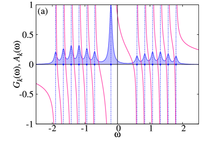
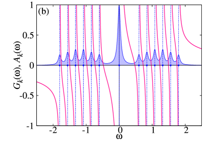
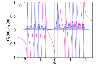
Figure 5: Schematic figures of $A_{\mathbf{k}}(\omega)=-{\rm Im}G_{\mathbf{k}}(\omega+i\delta^{+})/\pi$ (blue shaded region) and $G_{\mathbf{k}}(\omega)$ (red solid lines) at momentum $\mathbf{k}$ (a) inside, (b) on, and (c) outside the Fermi surface for a simple metal. Here $\omega=0$ corresponds to the Fermi energy. The poles of $G_{\mathbf{k}}(\omega)$ are indicated by dots along with dashed vertical lines.

Apparently, for momentum $\mathbf{k}$ on the Fermi surface, there exists a pole exactly at the chemical potential, i.e.,

$$\omega_{1}^{(\mathbf{k})}<\zeta_{1}^{(\mathbf{k})}<\cdots<\zeta_{m_{\rm FS}-1}^{(\mathbf{k})}<\omega_{m_{\rm FS}}^{(\mathbf{k})}=0<\zeta_{m_{\rm FS}}^{(\mathbf{k})}<\cdots,$$ (90)

with $n_{G^{-1}_{\mathbf{k}}}(\Gamma_{<})=0$ and $n_{G^{-1}_{\mathbf{k}}}(\Gamma_{0})=1$. Therefore, according to Eq. (77), this momentum contributes to the Luttinger volume $V_{\rm L}$ by one, including the spin degrees of freedom. Since $G_{\mathbf{k}}(0)$ exhibits a pole, its sign is not defined. A typical behavior of $A_{\mathbf{k}}(\omega)$ and $G_{\mathbf{k}}(\omega)$ is schematically shown in Fig. 5 (b).

For momentum $\mathbf{k}$ inside the Fermi surface, the topmost singularity of the Green’s function below the chemical potential must be a pole, i.e.,

$$\omega_{1}^{(\mathbf{k})}<\zeta_{1}^{(\mathbf{k})}<\cdots<\zeta_{m_{\rm top}-1}^{(\mathbf{k})}<\omega_{m_{\rm top}}^{(\mathbf{k})}<0<\zeta_{m_{\rm top}}^{(\mathbf{k})}<\cdots$$ (91)

because $G_{\mathbf{k}}(0)>0$. Since the number of poles below the chemical potential is larger than the number of zeros below the chemical potential exactly by one, it is shown that $n_{{{G}_{\mathbf{k}}^{-1}}}(\Gamma_{<})=1$ and $n_{{{G}_{\mathbf{k}}^{-1}}}(\Gamma_{0})=0$, and thus this momentum contributes to the Luttinger volume $V_{\rm L}$ by two, including the spin degrees of freedom [see Eq. (77)]. Recall here that in a simple metal such as Fermi liquid Landau1956 ; Nozieres1962 ; Luttinger1962 ; Pines the topmost pole at $\omega_{m_{\rm top}}^{(\mathbf{k})}$ below and in the vicinity of the chemical potential corresponds to the quasiparticle, and the other poles form the incoherent part of the single-particle excitation, as depicted in Fig. 5 (a).

For momentum $\mathbf{k}$ outside the Fermi surface, the number of poles below the chemical potential is exactly the same as the number of zeros below the chemical potential because

$$\omega_{1}^{(\mathbf{k})}<\zeta_{1}^{(\mathbf{k})}<\cdots<\omega_{m_{\rm bot}-1}^{(\mathbf{k})}<\zeta_{m_{\rm bot}-1}^{(\mathbf{k})}<0<\omega_{m_{\rm bot}}^{(\mathbf{k})}<\cdots,$$ (92)

satisfying that $G_{\mathbf{k}}(0)<0$, as shown in Fig. 5 (c). Therefore, $n_{G_{\mathbf{k}}^{-1}}(\Gamma_{<})=n_{G_{\mathbf{k}}^{-1}}(\Gamma_{0})=0$ and hence this momentum does not contribute to $V_{\rm L}$. The analytical properties of the single-particle Green’s function $G_{\mathbf{k}}(\omega)$ are summarized in Table 2. Since $G_{\mathbf{k}}^{-1}(0)=0$ for $\mathbf{k}$ on the Fermi surface and $\Theta_{c}(G_{\mathbf{k}}(0))=\Theta_{c}(G_{\mathbf{k}}^{-1}(0))$ for $|G_{\mathbf{k}}(0)|<\infty$, the Luttinger volume $V_{\rm L}$ in Eq. (77) can be given as

$$\lim_{T\rightarrow 0}V_{\rm L}=2\sum_{\mathbf{k}}\Theta_{\frac{1}{2}}\left(G_{\mathbf{k}}^{-1}(0)\right)$$ (93)

for a paramagnetic single-band system, where $\Theta_{c}(\omega)$ is defined in Eq. (57). Equation. (93) clearly shows that the Luttinger volume, defined as the winding number of the single-particle Green’s function in Eq. (77), indeed corresponds to the momentum volume surrounded by the Fermi surface, as expected for a simple metal.

Table 2: Analytical properties of the single-particle Green’s function $G_{\mathbf{k}}(\omega)$ for a simple metal. FS stands for Fermi surface. $n_{\mathbf{k}}^{(0)}$ is defined in Eq. (95).

location of ${\mathbf{k}}$	inside FS	on FS	outside FS
position of singularities	Eq. (91)	Eq. (90)	Eq. (92)
sign of $G_{\mathbf{k}}(0)$	$G_{\mathbf{k}}(0)>0$	$G_{\mathbf{k}}^{-1}(0)=0$	$G_{\mathbf{k}}(0)<0$
$n_{G_{\mathbf{k}}^{-1}}(\Gamma_{<})$	1	0	0
$n_{G_{\mathbf{k}}^{-1}}(\Gamma_{0})$	0	1	0
$n_{G_{\mathbf{k}}^{-1}}(\Gamma_{>})$	0	0	1
$n_{\mathbf{k}}^{(0)}$	1	1/2	0

If we assume that the shape of the Fermi surface does not change with and without introducing electron interactions, then obviously the analysis given above shows that $n_{D}(\Gamma_{<})=0$ and $n_{D}(\Gamma_{0})=0$, thus satisfying the condition of type I for the Luttinger theorem in Eq. (66). However, in general, the condition of type I can be satisfied even if electron interactions alter the shape of the Fermi surface. Thus, we now simply assume that the type-I condition in Eq. (66) is satisfied. Then, it follows immediately that in the zero-temperature limit

$$N=2\sum_{\mathbf{k}}\Theta_{\frac{1}{2}}\left(G_{\mathbf{k}}^{-1}(0)\right).$$ (94)

This is the well known expression of the Luttinger theorem Luttinger1960 ; AGD , originally proved by the many-body perturbation theory in which the second-term of the right-hand side in Eq. (36) vanishes under the assumption that the self-energy is regular at the chemical potential and thus the perturbation expansion is converged Luttinger-Ward1960 (see also Ref. Karlsson2016 ).

Let us now discuss how the condition in Eq. (66), obtained independently of the many-body perturbation theory, is related to Luttinger’s original statement Luttinger1960 . The first condition $n_{D}(\Gamma_{<})=0$ in Eq. (66) implies that the number of $\mathbf{k}$ points inside the Fermi surface remains the same with and without introducing electron interactions. This is exactly the original statement of the Luttinger theorem, “The interaction may deform the FS (Fermi surface), but it cannot change its volume” Luttinger1960 . The second condition $n_{D}(\Gamma_{0})=0$ in Eq. (66) implies that the number of zero-energy quasiparticle excitation, i.e., the number of ${\mathbf{k}}$ points on the Fermi surface, is unchanged by introducing electron interactions.

The implication of the second condition is seemingly stronger than the original statement of the Luttinger theorem. However, the essential point of the second condition is to prohibit the appearance of the zeros of the single-particle Green’s function, or equivalently the emergence of the poles of the self-energy, at the chemical potential by introducing electron interactions in order to ensure the convergence of the many-body perturbation theory. Therefore, the Luttinger theorem with the type-I condition in Eq. (66) falls into the original statement of the theorem by Luttinger Luttinger1960 .

We also note that, from Table 2, it is plausible to regard the quantity in the parentheses of Eq. (77), i.e.,

$$n^{(0)}_{\mathbf{k}}=n_{{G_{\mathbf{k}}^{-1}}}(\Gamma_{<})+\frac{1}{2}n_{{G_{\mathbf{k}}^{-1}}}(\Gamma_{0}),$$ (95)

as the distribution function of quasiparticles labeled by momentum $\mathbf{k}$ in the Fermi-liquid theory at zero temperature (see for example Eq. (1.1) of Ref. Luttinger1962 ). Thus, the winding number $n_{{G_{\mathbf{k}}^{-1}}}({\cal C})$ of the interacting single-particle Green’s function $G_{\mathbf{k}}(z)$ embodies the concept of the quasiparticle distribution function (not the bare particle one). Therefore, the Luttinger volume in the zero temperature limit, $\lim_{T\to 0}V_{\rm L}=2\sum_{\mathbf{k}}n^{(0)}_{\mathbf{k}}$, represents nothing but the number of quasiparticles. Recall now that in the Landau’s Fermi-liquid theory the number $N$ of particles is a priori assumed to be equal to the number of quasiparticles at zero temperature Landau1956 ; Luttinger1962 . Hence, the argument here guarantees this fundamental assumption of the Landau’s Fermi-liquid theory if the Luttinger theorem is valid since the theorem equates $N$ with the Luttinger volume. In Appendix C, we generalize $n_{\mathbf{k}}^{(0)}$ for finite (but still low) temperatures and discuss the physical meaning.

IV.3 type II: Mott insulator

As an example of type II for the generalized Luttinger theorem with $n_{D}(\Gamma_{0})\neq 0$　 in Eq. (68), let us consider a system where a metal-insulator transition is induced by introducing fermion interactions. In the noninteracting limit, there should exist zero-energy poles in $\det\boldsymbol{G}_{0}$ at the Fermi energy since the system is metallic. However, once the interactions are introduced and the metal-insulator transition occurs, these zero-energy poles are moved away from the chemical potential and replaced with the zeros of ${\det\boldsymbol{G}}(0)$ due to the appearance of poles in the self energy (for example, see Fig. 6). This immediately implies that $n_{D}(\Gamma_{0})\not=0$ because $n_{{\det\boldsymbol{G}^{-1}_{0}}}(\Gamma_{0})>n_{{\det\boldsymbol{G}^{-1}}}(\Gamma_{0})$, and thus the case where the metal-insulator transition is induced by introducing fermion interactions should in general corresponds to type II for the generalized Luttinger theorem when the theorem is valid.

To demonstrate this, here we calculate the single-particle Green’s function of the one-dimensional single-band Hubbard model at half-filling by using the CPT Senechal2000 ; Senechal2012 . The Hamiltonian is described as

$$H=-t\sum_{\langle i,j\rangle,\sigma}\left(c_{i\sigma}^{\dagger}c_{j\sigma}+{\rm H.c.}\right)$$ (96)

$$+U\sum_{i}n_{i\uparrow}n_{i\downarrow}-\mu\sum_{i,\sigma}n_{i\sigma},$$ (97)

where the sum in the first term of the right-hand side, indicated by $\langle i,j\rangle$, runs over all pairs of nearest neighbor sites $i$ and $j$ with the hopping integral $-t$. The on-site interaction interaction (chemical potential) is represented by $U$ ($\mu$) and $n_{i\sigma}=c_{i\sigma}^{\dagger}c_{i\sigma}$. We set $\mu=U/2$ at half-filling for which the particle-hole symmetry is preserved.

The CPT allows to approximately evaluate the single-particle Green’s function $G_{\mathbf{k}}(z)$ at any momentum ${\mathbf{k}}$ with arbitrary fine resolution from the numerically exact single-particle Green’s function of a small cluster Senechal2000 ; Senechal2012 . In the CPT, the infinitely large cluster on which $H$ is defined is divided into a set of identical clusters, each of which is described by the cluster Hamiltonian $H_{\rm c}$, the same Hamiltonian $H$ in Eq. (96) but with open-boundary conditions, and the single-particle Green’s function for $H$ is approximated as

$$G_{\mathbf{k}}(z)=\frac{1}{L_{\rm c}}\sum_{i,j}\mathrm{e}^{-\mathrm{i}\mathbf{k}\cdot{(\mathbf{r}_{i}-\mathbf{r}_{j})}}\left[{\boldsymbol{G}^{\prime}}^{-1}_{\sigma}(z)-\boldsymbol{V}_{\mathbf{k}}\right]^{-1}_{ij},$$ (98)

where $L_{\rm c}$ is the number of sites in the cluster and $\mathbf{r}_{i}$ denotes the spatial location of site $i\,(=1,2,\cdots,L_{\rm c})$ in the cluster. ${\boldsymbol{G}}^{\prime}_{\sigma}(z)$ is the exact single-particle Green’s function of the cluster, i.e.,

$$\left[{\boldsymbol{G}}^{\prime}_{\sigma}(z)\right]_{ij} = \langle 0|c_{i\sigma}\left[z-H_{\rm c}+E_{0}^{\rm c}\right]^{-1}c_{j\sigma}^{\dagger}|0\rangle$$ (99)

$$+ \langle 0|c^{\dagger}_{j\sigma}\left[z+H_{\rm c}-E_{0}^{\rm c}\right]^{-1}c_{i\sigma}|0\rangle.$$

where $|0\rangle$ is the ground state of $H_{\rm c}$ with the eigenvalue $E_{0}^{\rm c}$. $\left[\boldsymbol{V}_{\mathbf{k}}\right]_{ij}$ is the matrix element between sites $i$ and $j$ for the inter-cluster hopping term represented in momentum space.

We evaluate ${\boldsymbol{G}^{\prime}}_{\sigma}(z)$ for a one-dimensional 12-site cluster, i.e., $L_{\rm c}=12$, with the Lanczos exact-diagonalization method Dagotto1994 ; Weisse . Note that the single-particle Green’s function $G_{\mathbf{k}}(z)$ obtained by the CPT can be represented in the Lehmann representation Aichhorn2006 ; Senechal2012 and satisfies the spectral-weight sum rule in Eq. (5) with positive-definite spectral weight. Therefore, the CPT is an appropriate method to demonstrate the formalism derived in Sec. III.

To examine the analytical properties of the single-particle Green’s function $G_{\mathbf{k}}(z)$, here we calculate the single-particle spectral function $A_{\mathbf{k}}(\omega)$ defined in Eq. (89) and the imaginary part of the self-energy

$$S_{\mathbf{k}}(\omega)=-\frac{1}{\pi}{\rm Im}\Sigma_{\mathbf{k}}(\omega+\mathrm{i}\delta^{+})$$ (100)

where $\Sigma_{\mathbf{k}}(z)=z-2t\cos{k}-{G^{-1}_{\mathbf{k}}}(z)$. Since the singularities (i.e., poles and zeros) of the single-particle Green’s function $G_{\mathbf{k}}(z)$ in complex $z$ plane occur only in the real frequency $\omega$ axis, these two quantities $A_{\mathbf{k}}(\omega)$ and $S_{\mathbf{k}}(\omega)$ can capture the structure of poles and zeros of $G_{\mathbf{k}}(z)$: a divergence of $A_{\mathbf{k}}(\omega)$ [$S_{\mathbf{k}}(\omega)$] corresponds to a pole (zero) of $G_{\mathbf{k}}(\omega+\delta^{+})$ in the limit of $\delta^{+}\to 0$. The CPT has been employed to study intensively the single-particle excitation spectra $A_{\mathbf{k}}(\omega)$ of the one-dimensional Hubbard model Senechal2000 , and therefore we shall focus only on the analytical properties of $G_{\mathbf{k}}(\omega)$ in the following.

The results of $A_{\mathbf{k}}(\omega)$ and $S_{\mathbf{k}}(\omega)$ for $U=0$ and $U/t=6$ at zero temperature are shown in Figs. 6(a) and 6(b), respectively. Here, we set that $\delta^{+}/t=0.05$ and thus the diverging behavior of $A_{\mathbf{k}}(\omega)$ and $S_{\mathbf{k}}(\omega)$ is replaced by sharp peak structures. The value of $U/t=6$ is chosen merely for better visibility of the spectra, although the one-dimensional Hubbard model at half-filling is insulating for any $U\,(>0)$ Lieb1968 , which can be correctly reproduced by the CPT Senechal2012 .

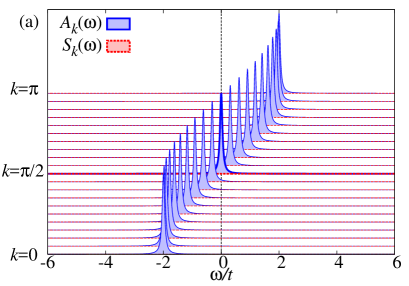
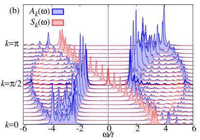
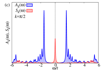
Figure 6: $A_{\mathbf{k}}(\omega)=-{\rm Im}G_{\mathbf{k}}(\omega+\mathrm{i}\delta^{+})/\pi$ (blue solid lines) and $S_{\mathbf{k}}(\omega)=-{\rm Im}\Sigma_{\mathbf{k}}(\omega+\mathrm{i}\delta^{+})/\pi$ (red dashed lines) of the one-dimensional single-band Hubbard model at half-filling for (a) $U=\mu=0$, (b) $U=2\mu=6t$, and (c) same as (b) but only for $k=\pi/2$. $\delta^{+}/t=0.05$ is set for all calculations. Note that different figures use different intensity scales. For visibility, $S_{\mathbf{k}}(\omega)$ is divided by $(U/t)^{2}$ in (b) and (c). The results for $k=\pi/2$ in (a) and (b) are indicated by thick lines.

For the noninteracting case, the Fermi points locate at $k=\pm\pi/2$ and the self-energy is zero by definition [see Fig. 6(a)]. On the other hand, for $U/t=6$, $A_{\mathbf{k}}(\omega)$ exhibits the single-particle excitation gap, as shown in Fig. 6(b). More interestingly, we find in Figs. 6(b) and 6(c) that a peak of $S_{\mathbf{k}}(\omega)$ intersects the zero energy, i.e., $\omega=0$, exactly at $k=\pm\pi/2$. Since the peak of $S_{\mathbf{k}}(\omega)$ corresponds to the zero of $G_{\mathbf{k}}(\omega)$, the result indicates that $G_{k=\pm\pi/2}(0)=0$. The momenta $k=\pi/2$ and $-\pi/2$ thereby form the Luttinger surface Dzyaloshinskii2003 , which is defined as a set of momenta $\mathbf{k}$ such that $G_{\mathbf{k}}(0)=0$. A typical behavior of $A_{\mathbf{k}}(\omega)$ and $G_{\mathbf{k}}(\omega)$ on the Luttinger surface is schematically shown in Fig. 7(b).

Because of $G_{\mathbf{k}}(0)=0$ on the Luttinger surface by definition, the order of singularities in $G_{\mathbf{k}}(\omega)$ for momentum ${\mathbf{k}}$ on the Luttinger surface must be

$$\omega_{1}^{(\mathbf{k})}<\zeta_{1}^{(\mathbf{k})}<\cdots<\omega_{m_{\rm LS}}^{(\mathbf{k})}<\zeta_{m_{\rm LS}}^{(\mathbf{k})}=0<\omega_{m_{\rm LS}+1}^{(\mathbf{k})}<\cdots,$$ (101)

where $\zeta_{m_{\rm LS}}^{(\mathbf{k})}$ is the $m_{\rm LS}$-th zero of $G_{\mathbf{k}}(\omega)$, i.e., $G_{\mathbf{k}}(\omega=\zeta_{m_{\rm LS}}^{(\mathbf{k})})=0$, and exactly zero note7 . Therefore, the number of poles $\{\omega^{(\mathbf{k})}_{1},\omega^{(\mathbf{k})}_{2},\dots\}$ below (above) the chemical potential is larger than the number of zeros $\{\zeta^{(\mathbf{k})}_{1},\zeta^{(\mathbf{k})}_{2},\dots\}$ below (above) the chemical potential by one. From Eqs. (79)–(81), we can now easily find that $n_{G^{-1}_{\mathbf{k}}}(\Gamma_{<})=n_{G^{-1}_{\mathbf{k}}}(\Gamma_{>})=1$ and $n_{G^{-1}_{\mathbf{k}}}(\Gamma_{0})=-1$, i.e., $n_{D_{\mathbf{k}}}(\Gamma_{<})=1$ and $n_{D_{\mathbf{k}}}(\Gamma_{0})=-2$, where $n_{D_{\mathbf{k}}}(\cal C)$ is given in Eq. (87). Thus, this momentum contributes to the Luttinger volume $V_{\rm L}$ by one, including the spin degree of freedom [see Eq. (77)].

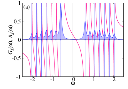
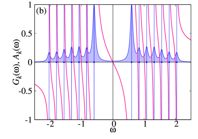
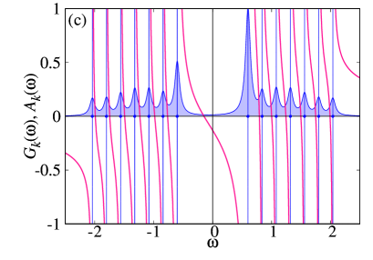
Figure 7: Schematic figures of $A_{\mathbf{k}}(\omega)=-{\rm Im}G_{\mathbf{k}}(\omega+i\delta^{+})/\pi$ (blue shaded region) and $G_{\mathbf{k}}(\omega)$ (red solid lines) with momentum $\mathbf{k}$ (a) inside, (b) on, and (c) outside the Luttinger surface for a Mott insulator. Here $\omega=0$ corresponds to the chemical potential in the zero-temperature limit. The poles of $G_{\mathbf{k}}(\omega)$ are indicated by dots along with dashed vertical lines.

We also find in Fig. 6(b) that the topmost (bottommost) singularity below (above) the chemical potential for $|k|<\pi/2$ is a pole of $A_{\mathbf{k}}(\omega)$ [$S_{\mathbf{k}}(\omega)$], implying that

$$\omega_{1}^{(\mathbf{k})}<\zeta_{1}^{(\mathbf{k})}<\cdots<\omega_{m_{\rm LS}^{\prime}}^{(\mathbf{k})}<0<\zeta_{m_{\rm LS}^{\prime}}^{(\mathbf{k})}<\omega_{m_{\rm LS}^{\prime}+1}^{(\mathbf{k})}<\cdots$$ (102)

and thus $G_{\mathbf{k}}(0)>0$ [see also Fig. 7(a)]. From Eqs. (79)–(81), we find that $n_{G^{-1}_{\mathbf{k}}}(\Gamma_{<})=1$ and $n_{G^{-1}_{\mathbf{k}}}(\Gamma_{0})=n_{G^{-1}_{\mathbf{k}}}(\Gamma_{>})=0$, which contributes two to the Luttinger volume $V_{\rm L}$ in the zero-temperature limit, including the spin degree of freedom. It is also apparent that $n_{D_{\mathbf{k}}}(\Gamma_{<})=n_{D_{\mathbf{k}}}(\Gamma_{0})=0$ for momentum below the Luttinger surface.

On the other hand, as shown in Fig. 6(b), the topmost (bottommost) singularity below (above) the chemical potential for $|k|>\pi/2$ is a pole of $S_{\mathbf{k}}(\omega)$ [$A_{\mathbf{k}}(\omega)$]. This implies that

$$\omega_{1}^{(\mathbf{k})}<\zeta_{1}^{(\mathbf{k})}<\cdots<\omega_{m_{\rm LS}^{\prime\prime}}^{(\mathbf{k})}<\zeta_{m_{\rm LS}^{\prime\prime}}^{(\mathbf{k})}<0<\omega_{m_{\rm LS}^{\prime\prime}+1}^{(\mathbf{k})}<\cdots$$ (103)

and thus $G_{\mathbf{k}}(0)<0$ [see also Fig. 7(c)]. From Eqs. (79)–(81), we find that $n_{G^{-1}_{\mathbf{k}}}(\Gamma_{<})=n_{G^{-1}_{\mathbf{k}}}(\Gamma_{0})=0$ and $n_{G^{-1}_{\mathbf{k}}}(\Gamma_{>})=1$, which contributes zero to the Luttinger volume $V_{\rm L}$ in the zero-temperature limit. These analytical properties of $G_{\mathbf{k}}(z)$ are summarized in Table 3.

Table 3: Analytical properties of the single-particle Green’s function $G_{\mathbf{k}}(\omega)$ for a Mott insulator. LS stands for Luttinger surface. $n_{\mathbf{k}}^{(0)}$ is defined in Eq. (95).

location of ${\mathbf{k}}$	inside LS	on LS	outside LS
position of singularities	Eq. (102)	Eq. (101)	Eq. (103)
sign of $G_{\mathbf{k}}(0)$	$G_{\mathbf{k}}(0)>0$	$G_{\mathbf{k}}(0)=0$	$G_{\mathbf{k}}(0)<0$
$n_{G_{\mathbf{k}}^{-1}}(\Gamma_{<})$	1	1	0
$n_{G_{\mathbf{k}}^{-1}}(\Gamma_{0})$	0	-1	0
$n_{G_{\mathbf{k}}^{-1}}(\Gamma_{>})$	0	1	1
$n_{\mathbf{k}}^{(0)}$	1	1/2	0

Counting the momentum volume surrounded by the Luttinger surface in Fig. 6, we can find that the Luttinger volume $V_{\rm L}$ is exactly $N$, the number of total electrons, therefore satisfying the generalized Luttinger theorem. Indeed, as discussed above, we also find from zeros and poles of the single-particle Green’s function that the type II condition is fulfilled, i.e., $n_{D}(\Gamma_{0})=-2n_{D}(\Gamma_{<})\neq 0$, where $n_{D}({\cal C})$ is given in Eq. (86). Since the system studied here is particle-hole symmetric, these results simply demonstrate the general statement in Sec. III.4.

Finally, it is instructive to directly count how many times $G_{\mathbf{k}}^{-1}(z)$ and $D_{\mathbf{k}}(z)$ wind around the origin in the complex $G_{\mathbf{k}}^{-1}$ and $D_{\mathbf{k}}$ planes, respectively, when $z$ moves along contour $\mathcal{C}$ shown in Fig. 2 (b). Recall that $n_{G_{\mathbf{k}}^{-1}}(\mathcal{C})$ and $n_{D_{\mathbf{k}}}(\mathcal{C})$ can be evaluated either by counting the number of zeros and poles of $G_{\mathbf{k}}(z)$, as shown above, or by directly counting the winding numbers of $G_{\mathbf{k}}^{-1}(z)$ and $D_{\mathbf{k}}(z)$ [see Eq. (78) and (85)]. For this purpose, it should be noted that as long as the poles and zeros are properly included, contour $\mathcal{C}$ ($=\Gamma_{0}$, $\Gamma_{<}$, and $\Gamma_{>}$) can be chosen rather freely. Therefore, as shown in Fig. 8, we consider the following contours

$$z=\left\{\begin{array}[]{ll}r_{0}\mathrm{e}^{\mathrm{i}\phi}&{\rm for}\,\,\Gamma_{0}\\ r_{<}\mathrm{e}^{\mathrm{i}\phi}-a&{\rm for}\,\,\Gamma_{<}\\ r_{>}\mathrm{e}^{\mathrm{i}\phi}+a&{\rm for}\,\,\Gamma_{>},\end{array}\right.$$ (107)

parametrized by angle $\phi$ ($-\pi<\phi\leq\pi$). Here, we set $r_{0}=t$, $r_{<}=r_{>}=2t$, and $a=3t$.

Figure 8: Contours $\Gamma_{0}$, $\Gamma_{<}$, and $\Gamma_{>}$ in the complex $z$ plane, parametrized by $\phi$ ($-\pi<\phi\leq\pi$), which correspond to those in Fig. 2(b).

Figure 9 summarizes the results for the trajectory of $G_{\mathbf{k}}^{-1}(z)$ in the complex ${G_{\mathbf{k}}^{-1}}$ plane at three representative momenta, i.e., $\mathbf{k}$ below, on, and above the Luttinger surface. Directly counting how many times and which direction the trajectory winds around the origin in the complex ${G_{\mathbf{k}}^{-1}}$ plane, we find in Fig. 9 that i) $n_{G_{\mathbf{k}}^{-1}}(\Gamma_{<})=1$ and $G_{\mathbf{k}}^{-1}(\Gamma_{0})=G_{\mathbf{k}}^{-1}(\Gamma_{>})=0$ for $\mathbf{k}$ below the Luttinger surface, ii) $n_{G_{\mathbf{k}}^{-1}}(\Gamma_{<})=G_{\mathbf{k}}^{-1}(\Gamma_{>})=1$ and $G_{\mathbf{k}}^{-1}(\Gamma_{0})=-1$ for $\mathbf{k}$ on the Luttinger surface, and iii) $n_{G_{\mathbf{k}}^{-1}}(\Gamma_{<})=G_{\mathbf{k}}^{-1}(\Gamma_{0})=0$ and $G_{\mathbf{k}}^{-1}(\Gamma_{>})=1$ for $\mathbf{k}$ above the Luttinger surface. These results are indeed exactly the same as those obtained above in Table 3 by counting the number of zeros and poles of $G_{\mathbf{k}}(z)$ given in Eqs. (101)–(103).

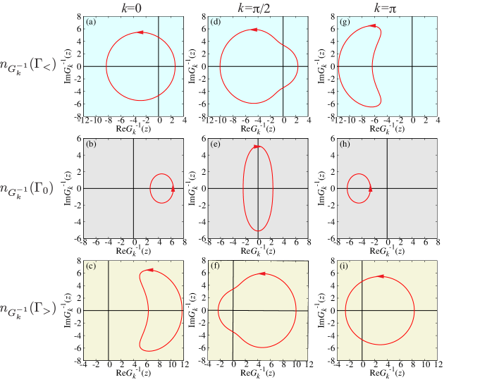
Figure 9: Trajectory of $G_{\mathbf{k}}^{-1}(z)$ in the complex $G_{\mathbf{k}}^{-1}$ plane when $z$ moves along contour $\mathcal{C}$ ($=\Gamma_{0}$, $\Gamma_{<}$, and $\Gamma_{>}$) given in Eq. (107) and also in Fig. 8 for three representative momenta, i.e., $k=0$ (inside the Luttinger surface), $k=\pi/2$ (on the Luttinger surface), and $k=\pi$ (outside the Luttinger surface). The CPT is employed for the one-dimensional one-band Hubbard model defined in Eq. (96) with $U/t=6$ at half-filling. By directly counting how many times and which direction (indicated by arrows) the trajectory winds around the origin in the complex $G_{\mathbf{k}}^{-1}$ plane, we find that (a) $n_{G_{k=0}^{-1}}(\Gamma_{<})=1$, (b) $n_{G_{k=0}^{-1}}(\Gamma_{0})=0$, (c) $n_{G_{k=0}^{-1}}(\Gamma_{>})=0$, (d) $n_{G_{k=\pi/2}^{-1}}(\Gamma_{<})=1$, (e) $n_{G_{k=\pi/2}^{-1}}(\Gamma_{0})=-1$, (f) $n_{G_{k=\pi/2}^{-1}}(\Gamma_{>})=1$, (g) $n_{G_{k=\pi}^{-1}}(\Gamma_{<})=0$, (h) $n_{G_{k=\pi}^{-1}}(\Gamma_{0})=0$, and (i) $n_{G_{k=\pi}^{-1}}(\Gamma_{>})=1$. These are exactly the same as those obtained by counting the number of poles and zeros of the single-particle Green’s function $G_{\mathbf{k}}(z)$ given in Eqs. (101)–(103) (see also Table 3).

Figure 10 shows the results for the trajectory of $D_{\mathbf{k}}(z)$ in the complex $D_{\mathbf{k}}$ plane at the three representative momenta. Counting how many times and which direction the trajectory winds around the origin in the complex $D_{\mathbf{k}}$ plane, we find in Fig. 10 that i) $n_{D_{\mathbf{k}}}(\Gamma_{<})=n_{D_{\mathbf{k}}}(\Gamma_{0})=n_{D_{\mathbf{k}}}(\Gamma_{>})=0$ for $\mathbf{k}$ below and above the Luttinger surface, and ii) $n_{D_{\mathbf{k}}}(\Gamma_{<})=n_{D_{\mathbf{k}}}(\Gamma_{>})=1$ and $n_{D_{\mathbf{k}}}(\Gamma_{0})=-2$ for $\mathbf{k}$ on the Luttinger surface. Therefore, we can show that $n_{D_{\mathbf{k}}}(\Gamma_{<})+\frac{1}{2}n_{D_{\mathbf{k}}}(\Gamma_{0})=0$ for each momentum ${\mathbf{k}}$ and hence the generalized Luttinger theorem is valid since $\lim_{T\to 0}\Delta V_{\rm L}=0$ [see Eq. (84)], the same conclusion reached above by counting the number of poles and zeros of $G_{\mathbf{k}}(z)$.

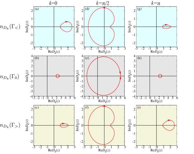
Figure 10: Trajectory of $D_{\mathbf{k}}(z)=G_{0{\mathbf{k}}}(z)/G_{\mathbf{k}}(z)$ in the complex $D_{\mathbf{k}}$ plane when $z$ moves along contour $\mathcal{C}$ ($=\Gamma_{0}$, $\Gamma_{<}$, and $\Gamma_{>}$) given in Eq. (107) and also in Fig. 8 for three representative momenta, i.e., $k=0$ (inside the Luttinger surface), $k=\pi/2$ (on the Luttinger surface), and $k=\pi$ (outside the Luttinger surface). The CPT is employed for the one-dimensional one-band Hubbard model defined in Eq. (96) with $U/t=6$ at half-filling. By directly counting how many times and which direction (indicated by arrows) the trajectory winds around the origin in the complex $D_{\mathbf{k}}$ plane, we find that (a) $n_{D_{k=0}}(\Gamma_{<})=0$, (b) $n_{D_{k=0}}(\Gamma_{0})=0$, (c) $n_{D_{k=0}}(\Gamma_{>})=0$, (d) $n_{D_{k=\pi/2}}(\Gamma_{<})=1$, (e) $n_{D_{k=\pi/2}}(\Gamma_{0})=-2$, (f) $n_{D_{k=\pi/2}}(\Gamma_{>})=1$, (g) $n_{D_{k=\pi}}(\Gamma_{<})=0$, (h) $n_{D_{k=\pi}}(\Gamma_{0})=0$, and (i) $n_{D_{k=\pi}}(\Gamma_{>})=0$. Notice that the trajectory winds twice around the origin in (e). Therefore, we find that $n_{D}(\Gamma_{0})=-2n_{D}(\Gamma_{<})=-4$, satisfying the condition of type II for the generalized Luttinger theorem in Eq. (68).

V Remarks

First, the sign of $G_{\mathbf{k}}(0)$ has been originally utilized to quantify interior and exterior of the Fermi or Luttinger surface Luttinger1960 ; Dzyaloshinskii2003 . However, as summarized in Tables 1, 2, and 3, $n^{(0)}_{\mathbf{k}}$ defined in Eq. (95) can also quantify the location of momentum $\mathbf{k}$ which may be inside, outside, or on the Fermi or Luttinger surface. Indeed, as already discussed in Sec. IV.2 (also see Appendix C), $n^{(0)}_{\mathbf{k}}$ can be interpreted as the quasiparticle distribution function in the Fermi-liquid theory. It should be emphasized that $n^{(0)}_{\mathbf{k}}$ itself has the topological nature since it is associated with the winding number of the single-particle Green’s function $G_{\mathbf{k}}(z)$.

Second, it is interesting to notice that the phase shift discussed in impurity scattering problems can be described with the similar form of Eqs. (61) and (64), where the scattering potential or $T$-matrix replaces the many body self-energy $\boldsymbol{\Sigma}(z)$. In the impurity scattering problems, the integer winding number $n_{D}({\mathcal{C}})$ corresponds to the number of bound states (Levinson’s theorem) Levinson1949 ; Dewitt1956 ; Schiff ; Umezawa1986 or the number of external charges (Friedel sum rule) Friedel1952 ; Langer1961 ; Doniach . Furthermore, according to the Levinson’s theorem, a fractional factor of $1/2$ should be added in the phase shift when a bound state exists at zero energy Schiff ; Umezawa1986 , which is again analogous to the fractional contribution to $\Delta V_{\rm L}$ in Eq. (63) when the determinant of the single-particle Green’s function exhibits singularities at the chemical potential.

Third, the topological aspect of the Luttinger theorem found here clearly differs from the topological approach to the Luttinger theorem reported in Ref. Oshikawa2000 . The main difference is twofold: (i) the topological nature examined and (ii) the resulting topological quantity. We have derived here the topological nature of the single-particle Green’s function for general systems, whereas in Ref. Oshikawa2000 the topological nature of the ground-state wave function is studied for Fermi liquids. We have shown that the winding number $n_{D}({\mathcal{C}})$ is the topological quantity which quantifies whether the generalized Luttinger theorem is valid. In Ref. Oshikawa2000 , the difference of the Fermi surface volume and the filling factor of a partially filled band is the topological quantity $n$, which is nothing but the number of completely filled bands. Therefore, $n=0$ corresponds to the case where no filling band exists and Luttinger theorem is always satisfied regardless of values of $n$. Note also that the topological approach in Ref. Oshikawa2000 is formulated for periodic systems with a particular set of system sizes, while our approach can be applied to general systems.

VI Summary and discussion

Based solely on analytical properties of the single-particle Green’s function of fermions at finite temperatures, we have shown that the Luttinger volume is represented as the winding number of (the determinant of) the single-particle Green’s functions. Therefore, this inherently introduces the topological interpretation of the generalized Luttinger theorem, and naturally leads to two types of conditions (types I and II) for the validity of the generalized Luttinger theorem. Type I falls into the Fermi-liquid case originally discussed by Luttinger in the 1960’s, where the Fermi surface is well defined at momenta where $G_{\mathbf{k}}(\omega=0)$ exhibits a pole. Type II includes the non-metallic case such as the Mott insulator to which Dzyaloshinskii has extended the Luttinger’s argument in the 2000’s by introducing the new concept of the Luttinger surface defined as a set of momenta where the sign of $G_{\mathbf{k}}(\omega=0)$ changes. We have also derived the sufficient condition for the validity of the Luttinger theorem of type I, representing the robustness of the theorem against the perturbation. We have also shown rigorously that the generalized Luttinger theorem of both types is valid for generic interacting fermions as long as the particle-hole symmetry is preserved. Moreover, we have shown that the winding number of the single-particle Green’s function can be considered as the distribution function of quasiparticles.

We should emphasize that these general statements can be made by noticing that the generalized Luttinger volume is expressed as the winding number of the single-particle Green’s function at finite temperatures, for which the complex analysis can be exploited readily and successfully without any ambiguity. This allows us to explore the intrinsic features of interacting fermions, independently of details of a microscopic Hamiltonian.

To be more specific in terms of these general analysis of interacting fermions, first we have examined the single-band simple metallic system with translational symmetry and discussed how the original statement of the theorem by Luttinger is understood with respect to our present analysis. We have also demonstrated our general analysis for a Mott insulator by examining the one-dimensional single-band Hubbard model at half-filling. Furthermore, using the Hubbard-I approximation, we have analyzed the half-filled Hubbard model on the honeycomb lattice where no apparent Fermi surface exists in the noninteracting limit.

It should be emphasized that the fermionic anti-commutation relation $\{c_{\alpha}^{\dagger},c_{\beta}\}=\delta_{\alpha\beta}$ plays a central role to determine the analytical properties of the single-particle Green’s function, including the asymptotic behavior for large $|z|$ and the number of zeros and poles of the single-particle Green’s function. Therefore, our analysis can also be extend to any fermionic systems with spin larger than 1/2. However, it is not straightforward to extend the present formalism to the $t$-$J$ model, which is a prototypical model of the strongly correlated electron systems studied extensively for cuprates Dagotto1994 . In the $t$-$J$ model, an electron moves between sites via the correlated hopping, represented in terms of the projected electron creation and annihilation operators to exclude the double occupancy. For example, the correlated hopping of an electron with spin $\sigma$ from site $j$ to site $i$ with hopping amplitude $t$ is expressed as

$$t{\bar{c}}_{i\sigma}^{\dagger}{\bar{c}}_{j\sigma} = t(1-{n}_{i\bar{\sigma}}){c}_{i\sigma}^{\dagger}{c}_{j\sigma}(1-{n}_{j\bar{\sigma}}),$$ (108)

where ${\bar{c}}^{\dagger}_{i\sigma}=(1-{n}_{i\bar{\sigma}}){c}_{i\sigma}^{\dagger}$ and ${\bar{c}}_{j\sigma}={c}_{j\sigma}(1-{n}_{j\bar{\sigma}})$ exclude the double occupancy on each site. Here, $\bar{\sigma}$ represents the opposite spin of $\sigma$. Since the projected electron creation and annihilation operators do not satisfy the anti-commutation relation, $\{\bar{c}_{\alpha}^{\dagger},\bar{c}_{\beta}\}\neq\delta_{\alpha\beta}$, we can no longer directly apply the same analytical argument of the single-particle Green’s function in Sec. II and Sec. III. Nonetheless, it is interesting to note that the violation of the Luttinger theorem in the two-dimensional $t$-$J$ model has been reported, based on the high-temperature expansion analysis of the momentum distribution function Putikka1998 and the exact-diagonalization analysis of the single-particle Green’s function for finite-size clusters Kokalj2007 , although the opposite had been concluded in the earlier study Stephan1991 .

Appendix A Another derivation of Eq. (36)

Here, we derive Eq. (36) from the derivative of the grand potential $\Omega$ with respect to the chemical potential $\mu$. As shown in the following, this alternative analysis reveals how the Legendre transform of the Luttinger-Ward functional, $\mathcal{F}$, is related to the deviation $\Delta V_{\rm L}$ of the Luttinger volume from the noninteracting one.

In the main text, we set the chemical potential $\mu$ as the origin of $z$ in the single-particle Green’s function $G_{\alpha\beta}(z)$ [Eq. (1)] by including $\mu$ in Hamiltonian $H$ (see Sec. II.1), and thus $z=0$ in $G_{\alpha\beta}(z)$ corresponding to the chemical potential. However, it is more useful to express $\mu$ explicitly in the formulae for the present purpose, and this can be done simply by replacing the Matsubara frequency $\mathrm{i}\omega_{\nu}$ with $\mu+\mathrm{i}\omega_{\nu}$:

$$\mathrm{i}\omega_{\nu}\rightarrow z_{\nu}=\mu+\mathrm{i}\omega_{\nu}.$$ (109)

The formulae return to those given in the main text by setting $\mu=0$ after the derivative with respect to $\mu$ is taken.

According to the self-energy-functional theory Potthoff2003 ; Potthoff2006 ; Potthoff2012 , the grand potential $\Omega$ is given as

$$\Omega=T\sum_{\nu=-\infty}^{\infty}\ln\det\boldsymbol{G}(z_{\nu})+\mathcal{F},$$ (110)

where $\mathcal{F}[\Sigma]$ is the Legendre transform of Luttinger-Ward functional $\Phi[\boldsymbol{G}]$ defined as

$$\mathcal{F}[\boldsymbol{\Sigma}]=\Phi[\boldsymbol{G}]-T\sum_{\nu=-\infty}^{\infty}\mathrm{e}^{\mathrm{i}\omega_{\nu}0^{+}}\mathrm{tr}[\boldsymbol{G}(\mathrm{i}\omega_{\nu})\boldsymbol{\Sigma}(\mathrm{i}\omega_{\nu})],$$ (111)

and all the quantities in Eq. (110) are given as $\Omega=\Omega[\boldsymbol{\Sigma}^{*}]$, $\boldsymbol{G}=\boldsymbol{G}[\boldsymbol{\Sigma}^{*}]$, and $\mathcal{F}=\mathcal{F}[\boldsymbol{\Sigma}^{*}]$ with the self-energy $\boldsymbol{\Sigma}^{*}$ which satisfies the stationary condition $\delta\Omega/\delta\boldsymbol{\Sigma}|_{\boldsymbol{\Sigma}=\boldsymbol{\Sigma}^{*}}=\boldsymbol{0}$. Note that, because $\Phi[\boldsymbol{G}]$ is the generating function of $\boldsymbol{\Sigma}$ Luttinger1960 ; Luttinger-Ward1960 , $\cal{F}[\boldsymbol{\Sigma}]$ is the generating function of $\boldsymbol{G}$,

$$\frac{\delta\mathcal{F}[\boldsymbol{\Sigma}]}{\delta{\Sigma}_{\alpha\beta}(z)}=-TG_{\beta\alpha}(z).$$ (112)

Thus we can show that

$$\frac{\delta\mathcal{F}[\boldsymbol{\Sigma}]}{\delta z}=\sum_{\alpha,\,\beta=1}^{L_{\rm s}}\frac{\delta\mathcal{F}[\boldsymbol{\Sigma}]}{\delta\Sigma_{\alpha\beta}}\frac{\delta\Sigma_{\alpha\beta}}{\delta z}=-T\mathrm{tr}\left[\boldsymbol{G}(z)\frac{\partial\boldsymbol{\Sigma}(z)}{\partial z}\right].$$ (113)

Applying $-\partial/\partial\mu$ in both sides of Eq. (110), we immediately find that the left-hand side gives the average particle number $N$, i.e.,

$$-\frac{\partial\Omega}{\partial\mu}=N,$$ (114)

whereas the first term of the right-hand side in Eq. (110) reads

$$- T\frac{\partial}{\partial\mu}\sum_{\nu=-\infty}^{\infty}\ln\det\boldsymbol{G}(z_{\nu})$$ (115)

$$= T\sum_{\nu=-\infty}^{\infty}\frac{\partial z_{\nu}}{\partial\mu}\frac{\partial}{\partial z_{\nu}}\ln\det\boldsymbol{G}(z_{\nu})^{-1}$$

$$= \oint_{\Gamma}\frac{\mathrm{d}z}{2\pi\mathrm{i}}n_{\rm F}(z-\mu)\frac{\partial\ln\det\boldsymbol{G}(z)^{-1}}{\partial z}=V_{\rm L}.$$

Here, contour $\Gamma$ is indicated in Fig. 2(a) with trivial modification due to non zero $\mu$ and Eq. (37) is used in the last equality.

Because the Luttinger volume of the noninteracting system $V_{\rm L}^{0}$ is $N$, we find form Eq. (110) that the deviation of the Luttinger volume from the noninteracting one, $\Delta V_{\rm L}$, is given as the derivative of the Legendre transform of the Luttinger-Ward functional, $\mathcal{F}$, with respect to $\mu$, i.e.,

$$\frac{\partial{\mathcal{F}}}{\partial\mu}=V_{\rm L}-N=\Delta V_{\rm L}.$$ (116)

Finally, $\partial\mathcal{F}/\partial\mu$ can also be directly evaluated as

$$\frac{\partial{\mathcal{F}}}{\partial\mu} = \sum_{\nu=-\infty}^{\infty}\frac{\delta\mathcal{F}}{\delta z_{\nu}}=-T\sum_{\nu=-\infty}^{\infty}{\rm tr}\left[\boldsymbol{G}(z)\frac{\partial\boldsymbol{\Sigma}(z)}{\partial z}\right]_{z=z_{\nu}}$$ (117)

$$= -\oint_{\Gamma}\frac{\mathrm{d}z}{2\pi\mathrm{i}}n_{\rm F}(z-\mu)\,{\rm tr}\left[\boldsymbol{G}(z)\frac{\partial\boldsymbol{\Sigma}(z)}{\partial z}\right]$$

where Eq. (113) is used in the second equality. Therefore, the first equality of Eq. (116) is nothing but Eq. (36) and thus we have proved that Eq. (36) can also be derived by the derivative of $\Omega$ with respect to $\mu$.

Appendix B Hubbard model on the honeycomb lattice: Hubbard-I approximation

The half-filled Hubbard model on the honeycomb lattice Sorella1992 ; Meng2010 ; Sorella2012 ; Otsuka2016 is a very instructive and yet non-trivial system to apply the analytical results in Sec. III because only the Fermi points exist in the two-dimensional Brillouin zone and hence the concept of “Fermi surface volume” is absent in the noninteracting limit.

B.1 Hubbard model on the honeycomb lattice

The Hubbard model on the honeycomb lattice is described by the following Hamiltonian:

$$H_{h}=H_{h}^{0}+U\sum_{i}\sum_{\xi=A,B}n_{i\xi\uparrow}n_{i\xi\downarrow},$$ (118)

where $H_{h}^{0}$ is the noninteracting tight-banding Hamiltonian on the honeycomb lattice,

$$H_{h}^{0}=\sum_{\mathbf{k}\sigma}\left(c_{\mathbf{k}A\sigma}^{\dagger},c_{\mathbf{k}B\sigma}^{\dagger}\right)\left(\begin{array}[]{cc}-\mu&\gamma_{\mathbf{k}}\\ \gamma_{\mathbf{k}}^{*}&-\mu\end{array}\right)\left(\begin{array}[]{c}c_{\mathbf{k}A\sigma}\\ c_{\mathbf{k}B\sigma}\end{array}\right).$$ (119)

Here, $c_{\mathbf{k}\xi\sigma}^{\dagger}=\frac{1}{\sqrt{L}}\sum_{i}c_{i\xi\sigma}^{\dagger}\mathrm{e}^{-{\mathrm{i}}\mathbf{k}\cdot\mathbf{r}_{i}}$ is the Fourier transform of an electron creation operator $c_{i\xi\sigma}^{\dagger}$ at the $i$-th unit cell, the location being denoted as ${\mathbf{r}}_{i}$ in real space, on sublattice $\xi\,(=A,B)$ with spin $\sigma\,(=\uparrow,\downarrow)$, and $\gamma_{\mathbf{k}}=-t(1+\mathrm{e}^{\mathrm{i}\mathbf{k}\cdot\mathbf{a}_{1}}+\mathrm{e}^{\mathrm{i}\mathbf{k}\cdot\mathbf{a}_{2}})$, where the hopping between the nearest neighbor sites is denoted as $-t$ and the primitive translational vectors are given as $\mathbf{a}_{1}=(1/2,\sqrt{3}/2)$ and $\mathbf{a}_{2}=(-1/2,\sqrt{3}/2)$, assuming that the lattice constant between the nearest neighbor sites is $1/\sqrt{3}$. The number of unit cells is $L$ and the chemical potential $\mu$ is explicitly included in $H_{h}^{0}$. $U$ is the on-site interaction and $n_{i\xi\sigma}=c^{\dagger}_{i\xi\sigma}c_{i\xi\sigma}$. Note that the particle-hole symmetry is preserved when $\mu=U/2$ at half-filling. The number $L_{\rm s}$ of the single-particle states labeled by $\alpha=(\mathbf{k},\sigma,\xi)$ (see Sec. II.1) is

$$L_{\rm s}=\sum_{\mathbf{k}}\sum_{\sigma=\uparrow,\downarrow}\sum_{\xi=A,B}=4L.$$ (120)

In the following of this Appendix, we only consider zero temperature.

B.2 Noninteracting limit

Let us first consider the noninteracting limit with $U=0$. As shown in Eq. (119), the noninteracting Hamiltonian $H_{h}^{0}$ is already diagonal with respect to momentum $\mathbf{k}$ and spin $\sigma$. Accordingly, the single-particle Green’s function ${\boldsymbol{G}}_{0}(z)$ is block diagonalized with respect to $\mathbf{k}$ and $\sigma$, and each element is denoted here as ${\boldsymbol{G}}_{0{\mathbf{k}}\sigma}(z)$. Since

$$\boldsymbol{G}_{0\mathbf{k}\sigma}(z)=\left(\begin{array}[]{cc}z+\mu&-\gamma_{\mathbf{k}}\\ -\gamma^{*}_{\mathbf{k}}&z+\mu\end{array}\right)^{-1},$$ (121)

we can readily show that

$$\det\boldsymbol{G}_{0\mathbf{k}\sigma}(z)=\left(\frac{1}{z+\mu-|\gamma_{\mathbf{k}}|}\right)\left(\frac{1}{z+\mu+|\gamma_{\mathbf{k}}|}\right)$$ (122)

for given $\mathbf{k}$ and $\sigma$. Notice that, because the single-particle energy dispersion $\pm|\gamma_{\mathbf{k}}|$ is $0$ at the $K$ and $K^{\prime}$ points (Dirac points), i.e., $\mathbf{k}=\frac{4\pi}{3}(\frac{1}{2},\frac{\sqrt{3}}{2})$ and $\frac{4\pi}{3}(-\frac{1}{2},\frac{\sqrt{3}}{2})$, respectively, $\det\boldsymbol{G}_{0\mathbf{k}\sigma}(z)$ has zero-energy poles at these momenta when $\mu=0$ at half-filling.

The determinant of the single-particle Green’s function is now evaluated as

$$\det\boldsymbol{G}_{0}(z)=\prod_{\boldsymbol{k}}\prod_{\sigma}\det\boldsymbol{G}_{0\mathbf{k}\sigma}(z)$$ (123)

$$= \left(\frac{1}{z+\mu}\right)^{8}\prod_{\mathbf{k}(\not=K,K^{\prime})}\left(\frac{1}{z+\mu-|\gamma_{\mathbf{k}}|}\right)^{2}\left(\frac{1}{z+\mu+|\gamma_{\mathbf{k}}|}\right)^{2}.$$

By counting the singularities as many times as its order, we find that at half-filling ($\mu=0$) the number of poles in $\det\boldsymbol{G}_{0}(z)$ at the chemical potential, corresponding to $z=0$, is 8 and the number of poles below the chemical potential is $2L-4$. Since $\det\boldsymbol{G}_{0}(z)$ has no zeros, i.e., $\det\boldsymbol{G}_{0}(z)\not=0$ for any $z$,

$$\left\{\begin{array}[]{l}n_{\det{\boldsymbol{G}}_{0}^{-1}}(\Gamma_{0})=8\\ n_{\det{\boldsymbol{G}}_{0}^{-1}}(\Gamma_{<})=2L-4\end{array}\right.$$ (126)

at half-filling [see Eqs. (51) and (52)]. Therefore, using Eq. (48), we find that $\lim_{T\to 0}V^{0}_{\rm L}=2L$. This is indeed expected for the noninteracting particle-hole symmetric systems since the number of electrons is $L_{\rm s}/2=2L$. However, we should note that this result is perhaps less obvious when we consider the Fermi surface volume because the Fermi surface here is composed of the Dirac points in the noninteracting limit at half-filling.

B.3 Hubbard-I approximation

Let us employ the Hubbard-I approximation Hubbard1963 to treat the on-site interaction at half-filling. In this approximation, the on-site interaction is approximated in the atomic limit with the self-energy ${\boldsymbol{\Sigma}}_{{\mathbf{k}}\sigma}(z)$ given as

$${\boldsymbol{\Sigma}}_{{\mathbf{k}}\sigma}(z)$$ (129)

$$= \left(\begin{array}[]{cc}Un_{A{\bar{\sigma}}}+\frac{U^{2}n_{A{\bar{\sigma}}}(1-n_{A{\bar{\sigma}}})}{z+\mu-U(1-n_{A{\bar{\sigma}}})}&0\\ 0&Un_{B{\bar{\sigma}}}+\frac{U^{2}n_{B{\bar{\sigma}}}(1-n_{B{\bar{\sigma}}})}{z+\mu-U(1-n_{B{\bar{\sigma}}})}\end{array}\right),$$

where $n_{\xi\sigma}$ is the average electron density on sublattice $\xi$ with spin $\sigma$, and $\bar{\sigma}$ indicates the opposite spin of $\sigma$. Noticing that $n_{A\sigma}=n_{B\sigma}=1/2$ at half-filling with the chemical potential $\mu=U/2$, the interacting single-particle Green’s function $\boldsymbol{G}_{\mathbf{k}\sigma}(z)$ for given $\mathbf{k}$ and $\sigma$ is now simply evaluated as

$$\boldsymbol{G}_{\mathbf{k}\sigma}(z) = \left[\boldsymbol{G}_{0\mathbf{k}\sigma}^{-1}(z)-\boldsymbol{\Sigma}_{\mathbf{k}\sigma}(z)\right]^{-1}$$ (132)

$$= \left(\begin{array}[]{cc}z-\frac{U^{2}}{4z}&-\gamma_{\mathbf{k}}\\ -\gamma^{*}_{\mathbf{k}}&z-\frac{U^{2}}{4z}\end{array}\right)^{-1}$$

and hence

$$\det\boldsymbol{G}_{\mathbf{k}\sigma}(z)=\frac{z^{2}}{(z-\omega_{\mathbf{k}}^{+})(z-\omega_{\mathbf{k}}^{-})(z+\omega_{\mathbf{k}}^{+})(z+\omega_{\mathbf{k}}^{-})}$$ (133)

with

$$\omega_{\mathbf{k}}^{\pm}=\frac{1}{2}\left(|\gamma_{\mathbf{k}}|\pm\sqrt{|\gamma_{\mathbf{k}}|^{2}+U^{2}}\right).$$ (134)

Therefore, the determinant of the interacting single-particle Green’s function $\boldsymbol{G}(z)$ is

$$\det\boldsymbol{G}(z) = \prod_{\mathbf{k}}\prod_{\sigma}\det\boldsymbol{G}_{\mathbf{k}\sigma}(z)$$ (135)

$$= z^{4L}\prod_{\mathbf{k}}\left(\frac{1}{z-\omega_{\mathbf{k}}^{+}}\right)^{2}\left(\frac{1}{z-\omega_{\mathbf{k}}^{-}}\right)^{2}$$

$$\times \left(\frac{1}{z+\omega_{\mathbf{k}}^{+}}\right)^{2}\left(\frac{1}{z+\omega_{\mathbf{k}}^{-}}\right)^{2}.$$

Since $\omega_{\boldsymbol{k}}^{+}>0$ and $\omega_{\boldsymbol{k}}^{-}<0$ for non-zero $U$, we find that the number of zeros of $\det\boldsymbol{G}(z)$ at (below) the chemical potential, corresponding to $z=0$, is $4L$ (0) and the number of poles of $\det\boldsymbol{G}(z)$ at (below) the chemical potential is 0 ($4L$). Thus, from Eqs. (51) and (52), we find that

$$\left\{\begin{array}[]{l}n_{\det{\boldsymbol{G}}^{-1}}(\Gamma_{0})=-4L\\ n_{\det{\boldsymbol{G}}^{-1}}(\Gamma_{<})=4L\end{array}\right.,$$ (138)

at half-filling. Using Eq. (48), we obtain that $\lim_{T\to 0}V_{\rm L}=2L$, thus satisfying the generalized Luttinger theorem.

Knowing the number of zeros and poles of $\det\boldsymbol{G}(z)$, the winding number $n_{D}({\mathcal{C}})$ [see Eq. (65)] of the Fredholm determinant $D(z)$ defined in Eq. (61) is now evaluated as

$$\left\{\begin{array}[]{l}n_{D}(\Gamma_{0})=-4L-8\\ n_{D}(\Gamma_{<})=2L+4\end{array}\right.,$$ (141)

which indeed fulfills the condition of type II for the validity of the generalized Luttinger theorem in Eq. (68) note8 . Note that in the Hubbard-I approximation the metal-insulator transition occurs as soon as a finite $U\,(>0)$ is introduced. Therefore, this example studied here also suggests that the (portion of) Fermi surface should disappear with the introduction of electron interactions when the condition of type II is satisfied.

B.4 Direct counting of winding numbers

As indicated in Fig. 3, the winding numbers, $n_{\det{\boldsymbol{G}}_{0}^{-1}}({\mathcal{C}})$ and $n_{\det{\boldsymbol{G}}^{-1}}({\mathcal{C}})$, can be evaluated directly by counting how many times and which direction $\det{\boldsymbol{G}}_{0}^{-1}(z)$ and $\det{\boldsymbol{G}}^{-1}(z)$ wind around the origin in the complex $\det{\boldsymbol{G}}_{0}^{-1}$ and $\det{\boldsymbol{G}}^{-1}$ planes, respectively, when $z$ moves along contour $\mathcal{C}$ shown in Fig. 2(b). Since it is instructive, here we shall evaluate directly the winding numbers within the Hubbard-I approximation by considering $3\times 3$ unit cells (i.e., $L=9$) with periodic boundary conditions, the smallest system size which contains both $K$ and $K^{\prime}$ points in the Brillouin zone, as shown in Fig. 11(a). The single-particle energy-dispersion relations for the noninteracting limit and for $U=5t$ are shown in Figs. 11(b) and 11(c), respectively. Since contour $\mathcal{C}$ can be chosen rather freely, as long as the poles and zeros are properly included, here we consider the contours given in Eq. (107) and in Fig. 8.

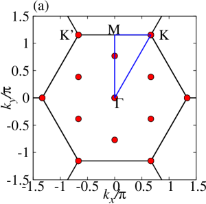
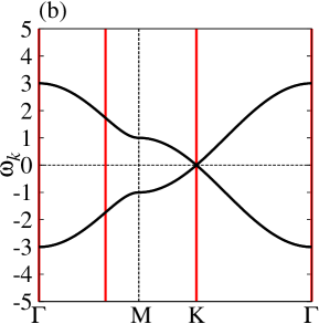
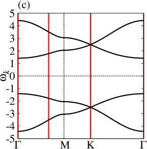
Figure 11: (a) The available $\mathbf{k}$ points (red solid circles) for the $3\times 3$ unit cell cluster of the honeycomb lattice with periodic boundary conditions. The black solid lines represent the boundaries of the Brillouin zone and the blue solid lines indicate the momentum path along which the single-particle energy-dispersion relations are shown in (b) and (c). Four high symmetric momenta are denoted as $\Gamma$: $(0,0)$, $K$: $(2\pi/3,2\pi/\sqrt{3})$, $M$: $(0,2\pi/\sqrt{3})$, and $K^{\prime}$: $(-2\pi/3,2\pi/\sqrt{3})$. (b) The single-particle energy-dispersion relation for $U=0$. (c) Same as (b) but for $U=5t$ obtained within the Hubbard-I approximation at half-filling. The red vertical lines in (b) and (c) represent the available $\mathbf{k}$ points for the $3\times 3$ unit cell cluster shown in (a).

Figures 12(a)–12(d) show the results of $\arg[\det\boldsymbol{G}_{0}^{-1}(z)]$ in the noninteracting limit and $\arg[\det\boldsymbol{G}^{-1}(z)]$ with $U=5t$ for $z$ along contours $\Gamma_{0}$ and $\Gamma_{<}$. Here, we have used $\det\boldsymbol{G}_{0}(z)$ and $\det\boldsymbol{G}(z)$ obtained analytically in Eqs. (123) and (135), respectively. Notice in these figures that the arguments of $\det\boldsymbol{G}_{0}^{-1}(z)$ and $\det\boldsymbol{G}^{-1}(z)$ are divided by $2$ [Figs. 12(a) and 12(b)] and 9 [Figs. 12(c) and 12(d)], respectively, for clarity. By directly counting how many times and which direction these quantities wind around the origin we find that $n_{\det\boldsymbol{G}_{0}^{-1}}(\Gamma_{0})/2=4$, $n_{\det\boldsymbol{G}_{0}^{-1}}(\Gamma_{<})/2=7$, $n_{\det\boldsymbol{G}^{-1}}(\Gamma_{0})/9=-4$, and $n_{\det\boldsymbol{G}^{-1}}(\Gamma_{<})/9=4$. These results are indeed the same as those obtained above in Eqs. (126) and (138) with $L=9$ by counting the number of zeros and poles of the determinant of the single-particle Green’s functions.

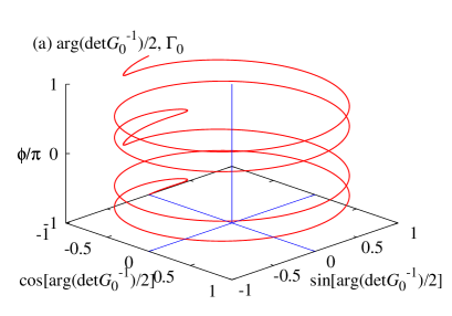
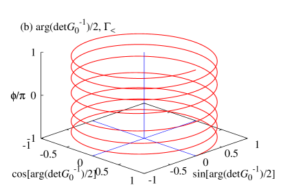
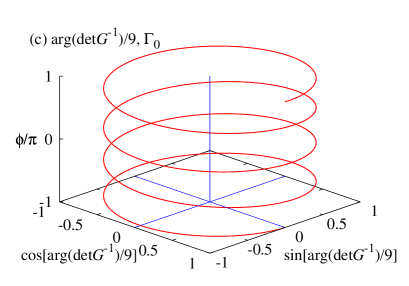
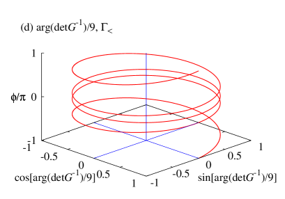
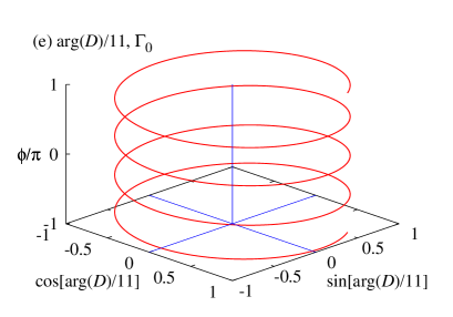
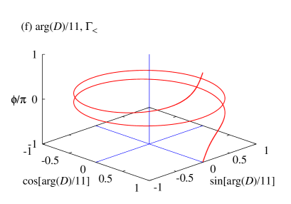
Figure 12: Arguments of $\det\boldsymbol{G}^{-1}(z)$ and $D(z)$ when $z$ moves along contour ${\mathcal{C}}\,(=\Gamma_{0}\,{\rm and}\,\Gamma_{<}\,{\rm in}\,{\rm Fig.~{}\ref{contour2}})$ for the Hubbard model on the honeycomb lattice with $3\times 3$ unit cells at half-filling. (a)–(d): $\arg[\det\boldsymbol{G}_{0}^{-1}(z)]$ for $z$ along contour $\Gamma_{0}$ (a) and $\Gamma_{<}$ (b) with $U=0$, and $\arg[\det\boldsymbol{G}^{-1}(z)]$ for $z$ along contour $\Gamma_{0}$ (c) and $\Gamma_{<}$ (d) with $U=5t$. (e) and (f): $\arg[D(z)]$ for $z$ along contour $\Gamma_{0}$ (e) and $\Gamma_{<}$ (f) with $U=5t$. Notice that the arguments are divided by 2, 9, or 11 (indicated in the figures), for clarity. The determinants of the single-particle Green’s functions, $\det\boldsymbol{G}_{0}(z)$ and $\det\boldsymbol{G}(z)$, are analytically given in Eqs. (123) and (135), respectively, and $D(z)=\det\boldsymbol{G}_{0}(z)/\det\boldsymbol{G}(z)$. By directly counting how many times and which directions these quantities wind around the origin while $\phi$ varies from $-\pi$ to $\pi$, we find that (a) $n_{\det\boldsymbol{G}_{0}^{-1}}(\Gamma_{0})/2=4$, (b) $n_{\det\boldsymbol{G}_{0}^{-1}}(\Gamma_{<})/2=7$, (c) $n_{\det\boldsymbol{G}^{-1}}(\Gamma_{0})/9=-4$, (d) $n_{\det\boldsymbol{G}^{-1}}(\Gamma_{<})/9=4$, (e) $n_{D}(\Gamma_{0})/11=-4$, and (f) $n_{D}(\Gamma_{<})/11=2$.

Similarly, $n_{D}({\mathcal{C}})$ in Eq. (64) can also be evaluated directly by counting how many times and which direction $D(z)$ winds around the origin in the complex $D$ plane, when $z$ moves along contour $\mathcal{C}$ shown in Fig. 8. The results of $\arg[D(z)]$ for $z$ along contours $\Gamma_{0}$ and $\Gamma_{<}$ with $U=5t$ are shown in Figs. 12(e) and 12(f), respectively. It is clearly observed in these figures that the winding numbers are $n_{D}(\Gamma_{0})/11=-4$ and $n_{D}(\Gamma_{<})/11=2$. These results are again comparable with those evaluated above in Eq. (141) with $L=9$ by counting the number of zeros and poles of the determinant of the single-particle Green’s functions. Indeed, we again find that $n_{D}(\Gamma_{<})+{\frac{1}{2}}n_{D}(\Gamma_{0})=0$, confirming the validity of the generalized Luttinger theorem with the condition of type II.

The analysis in this Appendix have clearly demonstrated that the formalism developed in Sec. III can apply without any ambiguity even to systems with point-like Fermi surfaces, where the concept of Fermi surface volume is obscure. We also note that the formalism developed in Sec. III can apply equally to, for example, particle-hole symmetric flat-band systems Lieb1989 ; Seki2016 where the entire Brillouin zone is covered with zero-energy poles of the single-particle Green’s function and thus the well-defined Fermi surface volume is absent in the noninteracting limit, and where the ground state might be ferrimagnetic when electron interactions are introduced.

Appendix C Quasiparticle distribution function at low temperatures

In this Appendix, we shall generalize the quasiparticle distribution function $n_{\mathbf{k}}^{(0)}$ [Eq. (95)] introduced in Sec. IV.2 to finite temperatures. For a paramagnetic single-band metallic system with translational symmetry, the Luttinger volume $V_{\rm L}$ at finite temperatures defined in Eq. (37) is given as

$$V_{\rm L}=2\sum_{\mathbf{k}}n_{\mathbf{k}},$$ (142)

where

$$n_{\mathbf{k}}=\sum_{m=1}^{P_{\mathbf{k}}}n_{\rm F}(\omega_{m}^{(\mathbf{k})})-\sum_{l=1}^{Z_{\mathbf{k}}}n_{\rm F}(\zeta_{l}^{(\mathbf{k})})$$ (143)

and the factor 2 in Eq. (142) is due to the spin degrees of freedom. Here, we have used Eqs. (38) and (40), and $P_{\mathbf{k}}$ ($Z_{\mathbf{k}}=P_{\mathbf{k}}-1$) is the number of poles (zeros) of the single-particle Green’s function $G_{\mathbf{k}}(\omega)$ for momentum $\mathbf{k}$ with spin $\sigma$ at finite temperatures [see Eqs. (73) and (75)]. In the zero-temperature limit, $n_{\mathbf{k}}$ reduces to the winding number $n_{\mathbf{k}}^{(0)}$ given in Eq. (95). Here, we argue that $n_{\mathbf{k}}$ defined in Eq. (143) can be considered as the quasiparticle distribution function in the Fermi-liquid theory at temperatures. In order to well define quasiparticles, the temperature has to be sufficiently low as compared with the quasiparticle excitation energy $\omega_{m_{\rm QP}}^{(\mathbf{k})}$ where $\omega_{m_{\rm QP}}^{(\mathbf{k})}$ is either $\omega_{m_{\rm top}}^{(\mathbf{k})}$, $\omega_{m_{\rm FS}}^{(\mathbf{k})}$, or $\omega_{m_{\rm bot}}^{(\mathbf{k})}$ in Eqs. (90)–(92), depending on momentum $\boldsymbol{k}$ (see Sec. IV.2 and Fig. 5). Since $\omega_{m_{\rm QP}}^{(\mathbf{k})}$ is bounded by $\zeta_{m_{\rm QP}-1}^{(\mathbf{k})}(<0)$ and $\zeta_{m_{\rm QP}}(>0)$ from the lower and upper sides, respectively, we will assume that temperature $T$ satisfies $T\ll\zeta_{m_{\rm QP}}^{(\mathbf{k})}-\zeta_{m_{\rm QP}-1}^{(\mathbf{k})}$, implying that

$$T\ll-\zeta_{m_{\rm QP}-1}^{(\mathbf{k})},\,\,\,\zeta_{m_{\rm QP}}^{(\mathbf{k})}.$$ (144)

Let us consider momentum $\mathbf{k}$ at which the singularities of $G_{\mathbf{k}}(\omega)$ are given as Eq. (91), i.e., $\mathbf{k}$ below the Fermi surface in the zero-temperature limit. Then we can write that

$$n_{\mathbf{k}}= n_{\rm F}(\omega_{m_{\rm top}}^{(\mathbf{k})})-\sum_{m=1}^{m_{\rm top}-1}\left[n_{\rm F}(\zeta_{m}^{(\mathbf{k})})-n_{\rm F}(\omega_{m}^{(\mathbf{k})})\right]$$ (145)

$$+ \sum_{m=m_{\rm top}}^{P_{\mathbf{k}}-1}\left[n_{\rm F}(\omega_{m+1}^{(\mathbf{k})})-n_{\rm F}(\zeta_{m}^{(\mathbf{k})})\right],$$

where the first term represents the contribution from the quasiparticle excitation, i.e., the topmost excitation below the chemical potential for which $G_{\mathbf{k}}(\omega)$ exhibits a pole, and the second (third) term from the incoherent part below (above) the chemical potential. In the following, we shall show that the contributions to $n_{\mathbf{k}}$ from the incoherent parts are exponentially small at low temperatures.

The second term on the right-hand side of Eq. (145) can be approximated as

$$\sum_{m=1}^{m_{\rm top}-1}\left(\zeta_{m}^{(\mathbf{k})}-\omega_{m}^{(\mathbf{k})}\right)\frac{n_{\rm F}(\zeta_{m}^{(\mathbf{k})})-n_{\rm F}(\omega_{m}^{(\mathbf{k})})}{\zeta_{m}^{(\mathbf{k})}-\omega_{m}^{(\mathbf{k})}}$$ (146)

$$\simeq \int_{\zeta_{1}^{(\mathbf{k})}}^{\zeta_{m_{\rm top}-1}^{(\mathbf{k})}}\mathrm{d}\omega\frac{\mathrm{d}n_{\rm F}(\omega)}{\mathrm{d}\omega}=n_{\rm F}(\zeta^{(\mathbf{k})}_{m_{\rm top}-1})-n_{\rm F}(\zeta_{1}^{(\mathbf{k})}).$$

Here, in the second line, we have assumed that each energy interval between the successive pole and zero, $\zeta_{m}^{(\mathbf{k})}-\omega_{m}^{(\mathbf{k})}$, in the incoherent part is small enough as compared with the whole energy width of the incoherent part itself, i.e., $\zeta^{(\mathbf{k})}_{m_{\rm top}-1}-\omega_{1}^{(\mathbf{k})}$. Similarly, the third term on the right-hand side of Eq. (145) can be approximated as

$$\sum_{m=m_{\rm top}}^{P_{\mathbf{k}}-1}\left[n_{\rm F}(\omega_{m+1}^{(\mathbf{k})})-n_{\rm F}(\zeta_{m}^{(\mathbf{k})})\right]\simeq n_{\rm F}(\zeta_{P_{\mathbf{k}}-1}^{(\mathbf{k})})-n_{\rm F}(\zeta^{(\mathbf{k})}_{m_{\rm top}}).$$ (147)

Since we assume that $T\ll\zeta_{m_{\rm top}}^{(\mathbf{k})}-\zeta_{m_{\rm top}-1}^{(\mathbf{k})}$, we can set that $n_{\rm F}(\zeta_{1}^{(\mathbf{k})})=1$ and $n_{\rm F}(\zeta_{P_{\mathbf{k}}-1}^{(\mathbf{k})})=0$ in Eqs. (146) and (147), respectively. Using $1-n_{\rm F}(z)=n_{\rm F}(-z)$, we thus find that

$$n_{\mathbf{k}} \simeq n_{\rm F}(\omega^{(\mathbf{k})}_{m_{\rm top}})+n_{\rm{F}}(-\zeta^{(\mathbf{k})}_{m_{\rm top}-1})-n_{\rm{F}}(\zeta^{(\mathbf{k})}_{m_{\rm top}})$$ (148)

$$= n_{\rm F}(\omega^{(\mathbf{k})}_{m_{\rm top}})+\mathcal{O}(\mathrm{e}^{\zeta^{(\mathbf{k})}_{m_{\rm top}-1}/T})-\mathcal{O}(\mathrm{e}^{-\zeta^{(\mathbf{k})}_{m_{\rm top}}/T}).$$

Note that the second and the third term in Eq. (148) are exponentially small because $T\ll-\zeta_{m_{\rm top}-1}^{(\mathbf{k})}$ and $T\ll\zeta_{m_{\rm top}}^{(\mathbf{k})}$ [see Eq. (144)].

Similarly, for momenta $\mathbf{k}$ at which singularities of $G_{\mathbf{k}}(\omega)$ are given as Eq. (90) (i.e., at the Fermi surface in the zero-temperature limit) and Eq. (92) (i.e., above the Fermi surface in the zero-temperature limit), we find that

$$n_{\mathbf{k}}\simeq n_{\rm F}(\omega^{(\mathbf{k})}_{m_{\rm FS}})+\mathcal{O}(\mathrm{e}^{\zeta^{(\mathbf{k})}_{m_{\rm FS}-1}/T})-\mathcal{O}(\mathrm{e}^{-\zeta^{(\mathbf{k})}_{m_{\rm FS}}/T})$$ (149)

and

$$n_{\mathbf{k}}\simeq n_{\rm F}(\omega^{(\mathbf{k})}_{m_{\rm bot}})+\mathcal{O}(\mathrm{e}^{\zeta^{(\mathbf{k})}_{m_{\rm bot}-1}/T})-\mathcal{O}(\mathrm{e}^{-\zeta^{(\mathbf{k})}_{m_{\rm bot}}/T}),$$ (150)

respectively. Here, the subscript $m_{\rm FS}$ should be read as a label for an excitation on the chemical potential because the Fermi surface is not well defined at finite temperatures. Equations (148)–(150) clearly show that $n_{\mathbf{k}}$ defined in Eq. (143) is expressed as the Fermi-Dirac distribution function $n_{\rm F}(\omega)$ of the quasiparticle excitation energy at momentum $\mathbf{k}$. Therefore, we can conclude that $n_{\mathbf{k}}$ is considered as the distribution function of quasiparticles at low temperatures.

Let us now consider $n_{\mathbf{k}}$ from the analytical aspects of the single-particle Green’s function $G_{\mathbf{k}}(z)$. As shown in Eq. (37), $n_{\mathbf{k}}$ in Eq. (143) is also expressed in the contour integral as

$$n_{\mathbf{k}}=\oint_{\Gamma}\frac{\mathrm{d}z}{2\pi\mathrm{i}}n_{\rm F}(z)\frac{\partial\ln G_{\mathbf{k}}^{-1}(z)}{\partial z}.$$ (151)

Explicitly considering the quasiparticle contribution in the single-particle Green’s function $G_{\mathbf{k}}(z)$, the Lehmann representation of $G_{\mathbf{k}}(z)$ [see Eq. (1)] is given as

$$G_{\mathbf{k}}(z)=\frac{a_{\mathbf{k}}}{z-\omega_{m_{\rm QP}}^{(\mathbf{k})}}+\sum_{m(\not={m_{\rm QP}})}^{P_{\mathbf{k}}}\frac{|Q_{\mathbf{k}m}|^{2}}{z-\omega_{m}^{(\mathbf{k})}},$$ (152)

where $\omega_{m_{\rm QP}}^{(\mathbf{k})}(=\omega_{m_{\rm top}}^{(\mathbf{k})},\omega_{m_{\rm FS}}^{(\mathbf{k})}$, or $\omega_{m_{\rm bot}}^{(\mathbf{k})})$ is the quasiparticle excitation energy for momentum ${\mathbf{k}}$ with the corresponding quasiparticle weight $a_{\mathbf{k}}=|Q_{\mathbf{k}{m_{\rm QP}}}|^{2}>0$, and the second term in the right-hand side represents the incoherent part of $G_{\mathbf{k}}(z)$.

When $z$ is in the vicinity of the quasiparticle excitation energy, i.e., $z\simeq\omega_{m_{\rm{QP}}}^{(\mathbf{k})}$, the single-particle Green’s function is approximated as $G_{\mathbf{k}}(z)\simeq a_{\mathbf{k}}/(z-\omega_{m_{\rm QP}}^{(\mathbf{k})})$ and thus we find that

$$\frac{\partial\ln G_{\mathbf{k}}^{-1}(z)}{\partial z}=G_{\mathbf{k}}(z)\frac{\partial G_{\mathbf{k}}^{-1}(z)}{\partial z}\simeq\frac{1}{z-\omega_{m_{\rm QP}}^{(\mathbf{k})}}.$$ (153)

This implies that the logarithmic derivative of $G_{\mathbf{k}}^{-1}(z)$ behaves like a free fermionic single-particle Green’s function with the excitation energy $\omega_{m_{\rm QP}}^{(\mathbf{k})}$ when $z\simeq\omega_{m_{\rm QP}}^{(\mathbf{k})}$. Therefore, the pole of the single-particle Green’s function at $\omega_{m_{\rm QP}}^{(\mathbf{k})}$ contributes to $n_{\mathbf{k}}$ in Eq. (151) by $n_{\rm F}(\omega_{m_{\rm{QP}}}^{(\mathbf{k})})$.

The same argument as in Eq. (153) can be applied to each of the remaining $P_{\mathbf{k}}-1$ poles of $G_{\mathbf{k}}(z)$, which are given in the second term of the right-hand side of Eq. (152). However, the positive contributions $n(\omega_{m}^{(\mathbf{k})})$ from these poles are mostly canceled by the negative contributions $-n(\zeta_{l}^{(\mathbf{k})})$ from the same number of zeros of $G_{\mathbf{k}}(z)$ at low temperatures, and thereby the net contribution to $n_{\mathbf{k}}$ from the remaining incoherent part is exponentially small. We thus again reach the same conclusion that

$$n_{\mathbf{k}}\simeq\oint\frac{\mathrm{d}z}{2\pi\mathrm{i}}n_{\rm F}(z)\frac{1}{z-\omega_{m_{\rm QP}}^{(\mathbf{k})}}=n_{\rm F}(\omega_{m_{\rm QP}}^{(\mathbf{k})}),$$ (154)

showing that $n_{\mathbf{k}}$ is dominated by the lowest-energy single-particle excitation $\omega_{m_{\rm QP}}^{(\mathbf{k})}$ and the excitation indeed obeys the Fermi-Dirac statistics, as in Eqs. (148)–(150).

The important consequence of this is that the Luttinger volume $V_{\rm L}$ in Eq. (142) provides the average number of quasiparticles. The Landau’s Fermi-liquid theory hypothesizes that the number of particles, $N$, is equal to that of quasiparticles Luttinger1962 . Therefore, the argument given here immediately implies that this fundamental hypothesis of the Landau’s Fermi-liquid theory is guaranteed when $V_{\rm L}=N$. This is the case when the Luttinger theorem is valid at zero temperature or when the particle-hole symmetry is preserved at finite temperatures, as shown in Eq. (71).

Finally, we note that for general complex frequency $z$,

$$\frac{\partial\ln G_{\mathbf{k}}^{-1}(z)}{\partial z}=G_{\mathbf{k}}(z)\Gamma_{\mathbf{k}}(z),$$ (155)

where $\Gamma_{\mathbf{k}}(z)=\frac{\partial G_{\mathbf{k}}^{-1}(z)}{\partial z}=1-\frac{\partial\boldsymbol{\Sigma}_{\mathbf{k}}(z)}{\partial z}$ is the scalar vertex function. The comparison with Eq. (153) suggests that $\Gamma_{\mathbf{k}}(z)$ enhances the renormalized quasiparticle spectral weight $a_{\mathbf{k}}(\leqslant 1)$ up to $1$ in the interacting single-particle Green’s function for $z$ near the quasiparticle excitation energy $\omega_{m_{\rm QP}}^{(\mathbf{k})}$. Notice also that Eq. (155) allows us for a diagrammatic representation of the Luttinger volume and the Luttinger theorem, as shown in Fig. 13.

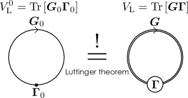
Figure 13: Diagrammatic representation for the Luttinger volumes of a noninteracting system $V_{\rm L}^{0}$ (left) and an interacting system $V_{\rm L}$ (right). Here, $\mathrm{Tr}[\cdots]=T\sum_{\nu=-\infty}^{\infty}\mathrm{e}^{\mathrm{i}\omega_{\nu}0^{+}}\mathrm{tr}[\cdots]$ and $\boldsymbol{\Gamma}_{0}=\frac{\partial\boldsymbol{G}_{0}^{-1}(z)}{\partial z}=\boldsymbol{I}$ (unit matrix). The thin line with an arrow represents $\boldsymbol{G}_{0}$, the dot $\boldsymbol{\Gamma}_{0}$, the double line with an arrow $\boldsymbol{G}$, and the circle $\boldsymbol{\Gamma}$. The Luttinger theorem equates these two quantities at zero temperature.

References

- (1) J. M. Luttinger, Fermi Surface and Some Simple Equilibrium Properties of a System of Interacting Fermions, Phys. Rev. 119, 1153 (1960).
- (2) J. M. Luttinger and J. C. Ward, Ground-State Energy of a Many-Fermion System. II, Phys. Rev. 118, 1417 (1960).
- (3) M. Oshikawa, Topological Approach to Luttinger’s Theorem and the Fermi Surface of a Kondo Lattice, Phys. Rev. Lett. 84, 3370 (2000).
- (4) A. A. Abrikosov, L. P. Gorkov, and I. E. Dzyaloshinski, Methods of quantum field theory in statistical physics (Dover publications, New York, 1975), Sec. 19.4, Chap. 4.
- (5) I. Dzyaloshinskii, Some consequences of the Luttinger theorem: The Luttinger surfaces in non-Fermi liquids and Mott insulators, Phys. Rev. B 68, 085113 (2003).
- (6) F. H. L. Essler and A. M. Tsvelik, Weakly coupled one-dimensional Mott insulators, Phys. Rev. B 65, 115117 (2002).
- (7) A. Rosch, Breakdown of Luttinger’s theorem in two-orbital Mott insulators, Eur. Phys. J. B. 59, 495 (2007).
- (8) J. Ortloff, M. Balzer, and M. Potthoff, Non-perturbative conserving approximations and Luttinger’s sum rule, Eur. Phys. J. B 58, 37 (2007).
- (9) M. Yamanaka, M. Oshikawa, and I. Affleck, Nonperturbative Approach to Luttinger’s Theorem in One Dimension, Phys. Rev. Lett. 79, 1110 (1997).
- (10) T. D. Stanescu, and G. Kotliar, Fermi arcs and hidden zeros of the Green function in the pseudogap state, Phys. Rev. B 74, 125110 (2006).
- (11) T. D. Stanescu, P. Phillips, and T.-P. Choy, Theory of the Luttinger surface in doped Mott insulators, Phys. Rev. B 75, 104503 (2007).
- (12) S. Sakai, Y. Motome, and M. Imada, Evolution of Electronic Structure of Doped Mott Insulators: Reconstruction of Poles and Zeros of Green’s Function, Phys. Rev. Lett. 102, 056404 (2009).
- (13) M. Imada, Y. Yamaji, S. Sakai, Y. Motome, Theory of pseudogap and superconductivity in doped Mott insulators, Ann. Phys., 523, 629 (2011).
- (14) R. Eder, K. Seki, and Y. Ohta, Self-energy and Fermi surface of the two-dimensional Hubbard model, Phys. Rev. B 83, 205137 (2011).
- (15) P. Phillips, Advanced solid state physics, Second edition (Cambridge University Press, Cambridge, 2012), Sec. 16.3, Chap. 16.
- (16) D. Sénéchal, D. Perez, and M. Pioro-Ladriere, Spectral Weight of the Hubbard Model through Cluster Perturbation Theory, Phys. Rev. Lett. 84, 522 (2000).
- (17) D. Sénéchal, Cluster perturbation theory in Strongly Correlated Systems, Springer Series in Solid-State Science, Vol. 171, edited by A. Avella and F. Mancini (Spinger, New York, 2012), Chap. 8.
- (18) M. Aichhorn, E. Arrigoni, M. Potthoff, and W. Hanke, Variational cluster approach to the Hubbard model: Phase-separation tendency and finite-size effects, Phys. Rev. B 74, 235117 (2006).
- (19) A. L. Fetter, and J. D. Walecka, Quantum thoery of many particle physics (Dover publications, New York, 2003), Sec. 31, Chap. 9.
- (20) The same pair of but with different order, i.e., , should be considered separately. In other words, in Eq. (1) should be considered simply as , and thus includes the case when .
- (21) J. M. Luttinger, Analytic Properties of Single-Particle Propagators for Many-Fermion Systems, Phys. Rev. 121, 942 (1961).
- (22) R. Eder, Comment on ‘Non-existence of the Luttinger-Ward functional and misleading convergence of skeleton diagrammatic series for Hubbard-like models’, arXiv:1407.6599.
- (23) K. Seki and S. Yunoki, Brillouin-zone integration scheme for many-body density of states: Tetrahedron method combined with cluster perturbation theory, Phys. Rev. B 93, 245115 (2016).
- (24) D. Karlsson and R. van Leeuwen, Partial self-consistency and analyticity in many-body perturbation theory: Particle number conservation and a generalized sum rule, Phys. Rev. B 94, 125124 (2016).
- (25) It should be noted that zeros of and at infinity () is not counted in and , respectively.
- (26) R. Eder, Correlated band structure of NiO, CoO, and MnO by variational cluster approximation, Phys. Rev. B 78, 115111 (2008).
- (27) See, for example, L. V. Ahlfors, Complex analysis, Third edition (McGraw-Hill, New York, 1979).
- (28) H. Ezawa, Y. Tomozawa, and H. Umezawa, Quantum statistics of fields and multiple production of mesons, Nuovo Cimento 5, 810 (1957).
- (29) T. Matsubara, A New Approach to Quantum-Statistical Mechanics, Prog. Theor. Phys. 14, 351 (1955).
- (30) B. L. Altshuler, A. V. Chubukov, A. Dashevskii, A. M. Finkelstein, and D. K. Morr, Luttinger theorem for a spin-density-wave state, Europhys. Lett. 41, 401 (1998).
- (31) For example, see F. Gebhard, The Mott Metal-Insulator Transition (Springer, Berlin, 1997), Sec. 2.5, Chap. 2.
- (32) Note that Eq. (71) is still correct even when a singularity appears at zero energy because .
- (33) L. D. Landau, The Theory of a Fermi Liquid, ZhETF 30, 1058 (1956) [J. Exptl. Theoret. Phys. 3, 920 (1956)].
- (34) P. Nozières and J. M. Luttinger, Derivation of the Landau Theory of Fermi Liquids. I. Formal Preliminaries, Phys. Rev. 127, 1423 (1962).
- (35) J. M. Luttinger and P. Nozières, Derivation of the Landau Theory of Fermi Liquids. II. Equilibrium Properties and Transport Equation, Phys. Rev. 127, 1431 (1962).
- (36) D. Pines and P. Nozières, The Theory of Quantum Liquids, Advanced Book Classics, (Perseus Books Publishing, Cambridge, Massachusetts, 1999), Chap. 1.
- (37) E. Dagotto, Correlated electrons in high-temperature superconductors, Rev. Mod. Phys. 66, 763 (1994).
- (38) A. Weiße and H. Fehske, Exact Diagonalization Techniques, in Computational Many-Particle Physics, edited by H. Fehske, R. Schneider, and A. Weiße, Springer Lecture Notes in Physics Vol. 739, 529 (Springer, Berlin, 2008).
- (39) E. H. Lieb and F. Y. Wu, Absence of Mott Transition in an Exact Solution of the Short-Range, One-Band Model in One Dimension, Phys. Rev. Lett. 20, 1445 (1968).
- (40) Note that the chemical potential should be determined by taking the zero-temperature limit becuase generally there is ambiguity in the chemical potential at exactly zero temperature for insulators.
- (41) N. Levinson, On the uniqueness of the potential in a Schrödinger equation for a given asymptotic phase, K. Dan. Vidensk. Selsk. Mat. Fys. Medd. 25, 9 (1949).
- (42) B. S. Dewitt, Transition from Discrete to Continuous Spectra, Phys. Rev. 103, 1565 (1956).
- (43) See, for example, L. I. Schiff, Quantum mechanics, Third edition (McGraw-Hill, New York, 1968), Sec. 39, Chap. 9.
- (44) H. Umezawa and G. Vitiello, Quantum Mechanics (Humanities Press, Leiden, 1986), Chap. 7.
- (45) J. Friedel, The distribution of electrons round impurities in monovalent metals, Phil. Mag. 43, 153 (1952).
- (46) J. S. Langer and V. Ambegaokar, Friedel Sum Rule for a System of Interacting Electrons, Phys. Rev. 121, 1090 (1961).
- (47) S. Doniach and E. H. Sondheimer, Green’s function for solid state physicists (Imperial College Press, London, 1998), Chap. 4.
- (48) W. O. Putikka, M. U. Luchini, and R. R. P. Singh, Violation of Luttinger’s Theorem in the Two-Dimensional - Model, Phys. Rev. Lett. 81, 2966 (1998).
- (49) J. Kokalj and P. Prelovšek, Luttinger sum rule for finite systems of correlated electrons, Phys. Rev. B 75, 045111 (2007).
- (50) W. Stephan and P. Horsch, Fermi surface and dynamics of the - model at moderate doping, Phys. Rev. Lett. 66, 2258 (1991).
- (51) M. Potthoff, Self-energy-functional approach to systems of correlated electrons, Eur. Phys. J. B 32, 429 (2003).
- (52) M. Potthoff, Non-perturbative construction of the Luttinger-Ward functional, Condens. Mat. Phys. 9, 557 (2006).
- (53) M. Potthoff, in Self-Energy-Functional Theory in Strongly Correlated Systems, edited by A. Avella and F. Mancini, Springer Series in Solid-State Science, Vol. 171, (Springer, Heidelberg, 2012) Chap. 10.
- (54) S. Sorella and E. Tosatti, Semi-Metal-Insulator Transition of the Hubbard Model in the Honeycomb Lattice, Europhys. Lett. 19, 699 (1992).
- (55) Z. Y. Meng, T. C. Lang, S. Wessel, F. F. Assaad, and A. Muramatsu, Quantum spin liquid emerging in two-dimensional correlated Dirac fermions, Nature 464, 847 (2010).
- (56) S. Sorella, Y. Otsuka, and S. Yunoki, Absence of a Spin Liquid Phase in the Hubbard Model on the Honeycomb Lattice, Sci. Rep. 2, 992 (2012).
- (57) Y. Otsuka, S. Yunoki, and S. Sorella, Universal Quantum criticality in the metal-insulator transition of two-dimensional interacting Dirac electrons, Phys. Rev. X 6, 011029 (2016).
- (58) J. Hubbard, Electron correlations in narrow energy bands, Proc. Roy. Soc. London A 276, 238 (1963).
-
(59)
Here, we have implicitly assumed in Eqs. (123) and (126)
that the Dirac points are among the allowed momenta for the honeycomb lattice
composed of finite sites.
However, this assumption is not essential for the conclusion.
If the Dirac points are not among the allowed momenta, poles of in the noninteracting limit
appears only above and below the chemical potential but not on the chemical potential, and thus we find that
at half-filling [for which the Luttinger volume in Eq. (48) is still ], while the analytic properties of remains the same as in Eqs. (135) and (138). Therefore, we find that(158)
and thus the condition of type II for the validity of the generalized Luttinger theorem is satisfied.(161) - (60) E. H. Lieb, Two theorems on the Hubbard model, Phys. Rev. Lett. 62, 1201 (1989).
- (61) K. Seki, T. Shirakawa, Q. Zhang, T. Li, and S. Yunoki, Emergence of massless Dirac quasiparticles in correlated hydrogenated graphene with broken sublattice symmetry, Phys. Rev. B 93, 155419 (2016).