Localization in One-Dimensional Tight-Binding Model with Chaotic Binary Sequences

Abstract

We have numerically investigated localization properties in the one-dimensional tight-binding model with chaotic binary on-site energy sequences generated by a modified Bernoulli map with the stationary-nonstationary chaotic transition (SNCT). The energy sequences in question might be characterized by their correlation parameter $B$ and the potential strength $W$. The quantum states resulting from such sequences have been characterized in the two ways: Lyapunov exponent at band centre and the dynamics of the initially localized wavepacket. Specifically, the $B-$dependence of the relevant Lyapunov exponent’s decay is changing from linear to exponential one around the SNCT ($B\simeq 2$). Moreover, here we show that even in the nonstationary regime, mean square displacement (MSD) of the wavepacket is noticeably suppressed in the long-time limit (dynamical localization). The $B-$dependence of the dynamical localization lengths determined by the MSD exhibits a clear change in the functional behaviour around SNCT, and its rapid increase gets much more moderate one for $B\geq 2$. Moreover we show that the localization dynamics for $B>3/2$ deviates from the one-parameter scaling of the localization in the transient region.

1 Introduction

It has been known that in one-dimensional disordered systems (1DDS) with uncorrelated on-site disorder all eigenstates are exponentially localized [1, 2, 3]. Still, for the 1D tight-binding model with potential sequences generated by Fourier filtering method (FFM) it has been known that correlations arising in the on-site potential delocalize the eigenstates and induce localization-delocalization transition (LDT) [4, 5, 6, 7, 8, 9, 10, 11, 12, 13, 14, 15, 16]. Indeed, the potential sequences involved ought to have long-range correlation with power spectrum $S(f)\sim 1/f^{\alpha}$ ($f<<1$, $\alpha\geq 2$), where $f$ denotes frequency and $\alpha$ is spectrum index. The potential sequence is non-stationary when the total power $\int_{0}^{\infty}S(f)df$ is divergent.

Noteworthy, the results do not contradict the Kotani theory of the localization stating that if the stationary random potential is non-deterministic, absolutely continuous spectrum is absent. The stationarity is a sufficient condition for the absence of absolutely continuous spectrum [17]. On the other hand, the potential sequence characterized by the power spectrum with the exponent $\alpha>1$ would be nonstationary. Further, most recent numerical studies show that the sequences with the power-law spectrum generated by Weierstrass function with fractal dimension $1<D<2$ induce the LDT [18, 19, 20, 21, 22].

There are systematic numerical studies for the above-mentioned 1DDS models with a potential to take continuous value like in the Anderson model. Whereas uncorrelated random model (e.g., Bernoulli Anderson model) with discretized values are well-known to show specific localization phenomena, the number of studies of localization and delocalization with the correlated binary potential are still few [24, 25, 26, 27, 28, 29, 30, 31]. E.g., among the latter examples the following one should be mentioned. There is a study of delocalization in binary ”0” and ”1” system and the sparse potential which takes different values for prime sites only [27]. It is in such a case that the very ”sparse” model should also naturally be ”nonstationary”. Remarkably, the existence of the LDT due to the potential intensity has also been demonstrated in the sparse impurity distance model [32].

Furthermore, a number of works also have been published on localized and delocalized phenomena in 1DDS with deterministic correlated sequence generated by chaotic map [24, 33, 34, 35, 36]. In our earlier papers, we also numerically investigated the localization and delocalization phenomena of binary random systems with long-range correlation by the modified Bernoulli map with stationary-nonstationary chaotic transition (SNCT) [24]. We shall refer to such a system MB system in the following [37, 25, 39]. The sequence becomes asymptotic non-stationary chaos for $\alpha>1$. In the MB system, it is possible to create the potential sequence that changes the property from short-range correlations including $\delta-$correlations to long-range correlation with a gentle change of the correlation parameter $B$. Meanwhile, studying in detail the modalities of the localization events, especially in the situations, where transitions from stationary ($3/2<B<2$) to nonstationary regime ($B>2$) regimen takes place in the binary correlated 1DDS has still not been enough. In particular, wavepacket dynamics in the nonstationary potential has hardly been investigated [44, 45, 46, 47, 48]. In this paper, we use the long-range correlated MB system having the binary potential sequence with taking either one of $-W$ or $W$, like in our previous papers. We aim at reporting the characteristic $B/W-$dependences of the Lyapunov exponent, the normalized localization length (NLL), and the quantum diffusion of the initially localized wavepacket around SNCT in binary correlated disordered systems.

This paper is organized as follows. In the next section, we shall briefly introduce the modified Bernoulli model. In Sect.3 we report about the global behaviour of the $B-$dependence and $N-$dependence of Lyapunov exponent and the NLL at band centre by the numerical calculation. While the Lyapunov exponent is positive throughout all the $B$ regions studied here, the Lyapunov exponent decreases linearly for $B<2$, but decays exponentially for $B>2$. As a result, the quantum states get delocalized ($\gamma_{N}\to 0$) with $B\to\infty$. In Sect.4, we report on the dynamical localization phenomena in the system. We find that the MSD is finite and dynamically localized in $t\to\infty$ even if the correlation parameter changes from stationary regime $B<2$ with power-law decay of the correlation to nonstationary regime ($B\geqq 2$). Its dynamical localization length (DLL) increases with the correlation parameter $B$, but the $B-$dependence changes from a relatively rapid increase to a more moderate one around SNCT($B\simeq 2$). The one-parameter scaling based on the localization length has large fluctuation in the transient region from ballistic motion to localization for $B>3/2$. The summary and discussion are presented in the last section. Appendix shows the sample fluctuation including nonstationary regime.

2 Model

We consider the one-dimensional tight-binding Hamiltonian describing single-particle electronic states as

$$H=\sum_{n=1}^{N}Wv(n)c_{n}^{\dagger}c_{n}+\sum_{n=1}^{N-1}c_{n}^{\dagger}c_{n+1}+H.C.,$$ (1)

where $c_{n}^{\dagger}$($c_{n}$) is the creation (annihilation) operator for an electron at site $n$. The $\{v_{n}\}_{n=0}^{N}$ and $W$ are the disordered on-site energy sequence and the strength, respectively. The amplitude of the quantum state $|\Phi>$ is given by $\phi(n)\equiv<\Phi|c_{n}^{\dagger}c_{n}|\Phi>$ in the site representation. To model the correlated disorder potential for $v_{n}$($n\leq N$) in Eq.(1), we use the modified Bernoulli map;

$$X_{n+1}=$$

$$\begin{cases}X_{n}+2^{B-1}(1-2b)X_{n}^{B}+b&(0\leq X_{n}<1/2)\\ X_{n}-2^{B-1}(1-2b)(1-X_{n})^{B}-b&(1/2\leq X_{n}\leq 1),\end{cases}$$ (2)

where $B$ is a bifurcation parameter which controls the correlation of the sequence. $b$ stands for the small perturbation which is set $b=10^{-13}$ in this paper. The map has been introduced to investigate the basic property of the intermittent chaos by Aizawa [37].

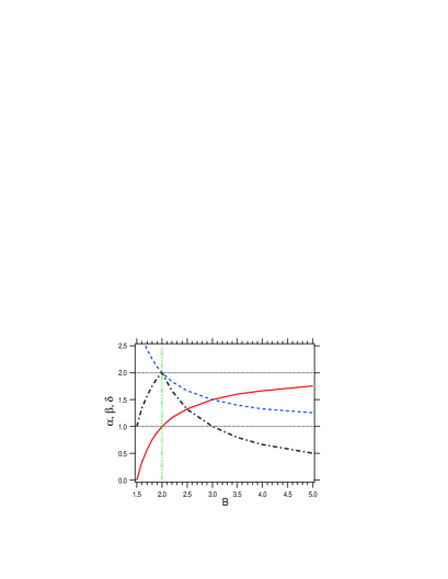
Figure 1: (Color online) Spectral index $\alpha$ (red solid line), index $\beta$ (blue broken line) of the residence time distribution, and $\delta$ (black dotted-dashed line) of the variance of the renewal process as a function of correlation parameter $B$. The black dotted lines denote $\alpha=2(=\alpha_{c})$ and $\beta=1(=\beta_{c})$ in a limit $B\to\infty$. The vertical double dotted-dashed (green) line denotes the SNCT $B=2$. In the present paper localization phenomena in a range $B\in[1.5,3.5]$ is mainly investigated.

The sequence is stationary for $B<2$ and nonstationary for $B\geq 2$. The stationary property is recovered by the perturbation though the essential property remains invariant for a long time $n<n_{b}$, where $n_{b}\simeq(2b)^{(1-B)/B}$ [37]. We use the course-grained binary sequence $\{v_{n}\}$ by the following rule:

$$\begin{cases}0\leq X_{n}<1/2&\to v_{n}=-1\\ 1/2\leq X_{n}<1&\to v_{n}=1.\end{cases}$$ (3)

Accordingly, the statistical property of the binary sequence can be characterized by changing the correlation parameter $B$. The following properties, for example, are analytically and numerically derived. In the stationary regime ($3/2<B<2$) the correlation function of the symbolic sequence decreases obeying the inverse-power law with the long-range correlation for large $n$ [37],

$$C(n)\equiv<v_{n_{0}+n}v_{n_{0}}>\sim n^{-\frac{2-B}{B-1}}(n>>1).$$ (4)

The correlation shows the critical decay $C(n)\sim 1/n$ at $B=3/2$. In the nonstationary regime ($B\geq 2$) the correlation decays as,

$$C(n)\simeq 1-\frac{2}{B}(\frac{n}{n_{b}})^{\frac{B-2}{B-1}},$$ (5)

for $n\leq n_{b}$. The power spectrum $S(f)=\frac{1}{N}\left|\sum_{n=0}^{N}e^{-i2\pi fn/N}\right|^{2}$ ($f=0,1,2,...,N-1$) in the low frequency limit behaves

$$S(f)\sim\begin{cases}f^{0}&1\leq B<3/2\\ f^{-\alpha}&3/2\leq B\leq\infty,\end{cases}$$ (6)

in the thermodynamic limit ($N\to\infty$), where

$$\alpha\simeq\frac{2B-3}{B-1}.$$ (7)

That is, the stationary sequence changes to nonstationary one with $S(f)\sim 1/f$ around $B\simeq 2$. It is suggested that in FFM model and Weierstrass model with long-range correlation LDT appear in a case with $\alpha\simeq 2$. Note that if $B\to\infty$, then $S(f)\sim f^{-2}$ as shown in Fig.1. Still, the localization property of 1DDS around $\alpha\simeq 1$ have not yet been studied. In the present paper, we investigate the change of the quantum states around the SNCT of the sequenece. It has already been reported that this property of the sequence strongly affects the statistical nature of the Lyapunov exponents of the electronic wave functions [24].

Moreover, the binary sequence $\{v_{n}\}$ can be recast as $\{(m_{0},\sigma),(m_{1},-\sigma),(m_{2},\sigma),(m_{3},-\sigma).....\}$. Here $(m_{k},\sigma)$ stands for the $m_{k}$ times iterating of one and the same symbol $\sigma$, where $\sigma$ represents $-1$ or $1$. The sequence is uniquely determined by the cluster size distribution $P(m)$ for the number $m$ of iterations in the pure sequence $(m,\sigma)$, which is independent of the value of the symbol. Hence, the time interval $m$ between successive renewal events is a random variable, whose probability density function $P(m)$:

$$P(m)\sim m^{-\beta},$$ (8)

where

$$\beta=\frac{B}{B-1}.$$ (9)

When $B<2$ the cluster size is finite ($<m><\infty$), and when $B\geq 2$ it diverges. It is worth noting that in the stationary regime ($B<2$) the normalized stationary distribution (invariant measure) exists; on the other hand, when $B\geq 2$ the sequence becomes nonstationary and the normalizable measure does not exist when $b=0$. If the perturbation $b$ is not introduced, the sequence is constructed by only the pure cluster of the same type symbol with probability one for the nonstationary regime.

The number of the renewal events $N_{t}$ in the interval $[0,t]$ can be approximated by renewal process. Then the variance $Var(N_{t})=<(N_{t}-<N_{t}>)^{2}>$($\sim t^{\delta}$) behaves as $\delta=4-\beta(3/2<B<2)$, $\delta=2\beta-2$($B\geqq 2$) depending on the parameter $B$ [38, 39]. (See Fig.1 for the $B-$dependence of the exponent $\delta$.) Indeed, it has been shown numerically that $B-$dependence of the exponent $\delta$ becomes maximum at $B=2$ and then decreases. We examine the localization property around the transition point ($B\simeq 2$) in potential sequence.

3 Lyapunov exponent and normalized localization length

The ensemble-averaged finite size Lyapunov exponent is defined by

$$\gamma_{N} = \left<\frac{\ln\left(|\phi(N)|^{2}+|\phi(N+1)|^{2}\right)}{2N}\right>,$$ (10)

for $N>>1$, where $\left<...\right>$ denotes the ensemble average over uniformly distributed initial value $X_{0}\in[0,1]$ in Eq.(2). We obtained the finite size Lyapunov exponent by standard transfer matrix products with the initial state $\phi(0)=\phi(1)=1$ [40]. Then $\xi(N)(=\gamma_{N}^{-1})$ denotes the finite size localization length (LL). We define the NLL to characterize the tail of the wavefunction,

$$\Lambda_{N}\equiv\frac{\xi(N)}{N}.$$ (11)

It is useful to study the localization and delocalization property that $\Lambda_{N}$ decreases (increases) with the system size $N$ for localized (extended) states, and it becomes constant for the critical states. In what follows, we investigate the NLL by changing the system size $N$ and the correlation parameter $B$ for the band centre $E=0$. The typical size $N$ and ensemble size used here are $N=2^{16}\sim 2^{23}$ and $2^{10}\sim 2^{12}$, respectively. The robustness of the numerical calculations has been confirmed in each case.

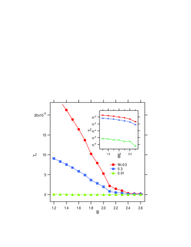
Figure 2: (Color online) Lyapunov exponent $\gamma_{N}$ in the band centre ($E=0$) as a function of the correlation parameter $B$ for $W=0.5,0.3,0.01$. $N=2^{23}$ and the sample size is $2^{12}$. The inset of the panel is semi-log plot.

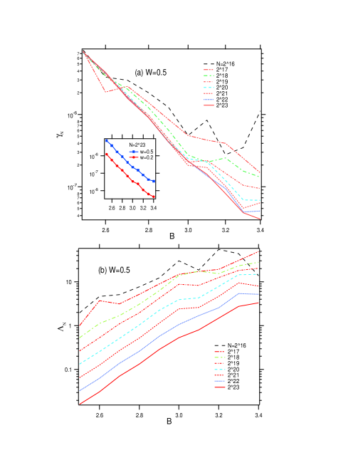
Figure 3: (Color online) (a)Lyapunov exponent $\gamma_{N}$ and (b)the normalized localization length $\Lambda_{N}$ as a function of the correlation parameter $B$ for several system size $N=2^{16}-2^{23}$. $W=0.5$, $E=0$, .and the sample size is $2^{12}$. Note that the vertical axis is in logarithmic plot. The inset of the panel (a) is result for $W=0.5$ and $W=0.2$ for $N=2^{23}$. The slope is about $-6.38$ in the semi-logarithmic plot.

3.1 A transition at $B\simeq 2$

As shown in Fig.2, for $1.2<B<2$ the Lyapunov exponent $\gamma_{N}$ monotonically decreases toward zero around $B=2$, and the $B-$dependence is roughly estimated as

$$\gamma_{N}\simeq\gamma_{0}(W)-k(W)B,$$ (12)

where $\gamma_{0}(W)$ and $k(W)$ are $W-$dependent coefficients. The tendency is almost independent of the potential strength $W$. In what following we show the more details numerical results for the nonstationary regime $B\geqq 2$.

Figure 3(a) shows the $B-$dependence of the Lyapunov exponent for the different system size with a fixed value $W=0.5$. As the system size grows, the $B-$dependence of $\gamma_{N}$ for $B\geq 2$ shows stable exponential decay such as:

$$\gamma_{N}(W,B)\simeq\gamma_{c}(W){\rm exp}\{-cB\},$$ (13)

where $\gamma_{c}(W)$ is the coefficient of dependence on $W$, and $c=6.38$ numerically. Moreover, from the comparison with the case of $W=0.2$ shown in the inset, it turns out that the decay rate (slope) hardly depends on the potential intensity $W$. That is, $B\to\infty$ is expected to be $\gamma_{N}\sim 0$ corresponding to the delocalized state.

Therefore, it seems that with the increase of $B$ the Lyapunov exponent shifts from a linear-decay to an exponential-decay in the MB quantum system with the potential sequence $v_{n}$. The property corresponds to the change of the potential sequence from the non-Gaussian stationary process to the nonstationary process at $B=2$. As to cover the anomalous fluctuation of the classical system by the quantum effect, the result of the quantum system is that the Lyapunov exponent is still positive (i.e. the localization length of the initially localized wavepacket is finite). In addition, the NLL $\Lambda_{N}$ is shown in Fig.3(b) in order to investigate the details of the size effect on the localized states for $B\geqq 2$. Accordingly, as we can infer from the behaviour of $\gamma_{N}$, the NLL also has an exponential dependence on $B$.

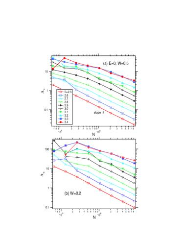
Figure 4: (Color online) The normalized localization length $\Lambda_{N}$ as a function of the system size $N$ for (a)$W=0.5$, (b) $W=0.2$. The other parameters are the same as Fig.3. Note that all axes are in logarithmic scale.

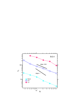
Figure 5: (Color online) The normalized localization length $\Lambda_{N}$ as a function of the system size $N$ for $B=3.4$ with $W=0.1,0.2,0.5$. Note that both axes are in logarithmic scale. The lines with slope $-1$ and $-0.64$ are shown as a reference.

3.2 Power-law localized behaviour

Figure 4 shows the $N-$dependence of NLL. In the case of $B=2.5$, it obviously declines with $N^{-1}$ irrespective of $W=0.5,0.2$. This corresponds to the clearly exponential localization at this system size, as could be seen from the definite value of $\gamma_{N}>0$. On the other hand, as $B$ increases, a tendency to decrease with the exponent $0<\eta<1$ can be seen as

$$\Lambda_{N}\sim N^{-\eta}.$$ (14)

Figure 5 shows $N-$dependence of $\Lambda_{N}$ for some $W$ with $B=3.4$. Estimating these slopes by the least-squares method shows that $\eta\simeq 0.64$ is almost independent of the value of $W$. Although this behaviour remains present until the infinity of $N$, the wavefunction might still be normalized in this region, and behave like power-law localized states with the point spectrum since $\delta>0.5$. However, there is a possibility that exists a characteristic length separating the outer exponential decay from the inner power-law decay of the localized states as in two-dimensional disordered systems with large localization length. That is, the wavefunction is power-law decay inside the localization length and exponential decay in the outside. It should be noticed as well, that the power-law behaviour with $0<\eta<1$ is observed as a transient phenomenon asymptotically going to $N^{-1}$ ($\eta=1$) for $N\to\infty$. Detailed calculations with larger system size are required for the definite conclusions.

4 Quantum wavepacket dynamics

This is just the main section of the present paper. LDT has been observed in phase space $(\alpha,W)$ and $(D,W)$ based on the Lyapunov exponent and/or NLL with FFM potential and Weierstrass potential, respectively. However, the effect of the long-range correlation on quantum diffusion in the 1DDS have not sufficiently been studied yet in 1DDS with long-range correlation. In this section, we examine the dynamical property of the initially localized wave packet by changing the parameter $B$ and $W$, but how would the SNCT characterized by the $1/f$ fluctuation influence on the localization property of the quantum states? Generally speaking, the positive Lyapunov exponent value does not seem to be the sole sufficient condition for the dynamical localization to occur. Hence, it turns out that directly studying the wavepacket dynamics is very important.

4.1 Method

The quantum time-evolution is given by

$$i\hbar\frac{\partial\phi(n,t)}{\partial t}=\phi(n+1,t)+\phi(n-1,t)+Wv(n)\phi(n,t),$$ (15)

where $n=1,2,...,N$. We take the initial state to be localized at the centre of the system, $\phi(n,t=0)=\delta_{n,N/2}$, and $\hbar=1$ throughout this calculation. In the numerical calculation we used FFT-symplectic integrator (SI) scheme for integrating the time-dependent Schrödinger equation [41, 42]. Then, we adapted periodic boundary condition because we used the FFT and inverse FFT to exchange the real space representation for the momentum space one and do the opposite operation. However, here we only consider the time periods, when the boundary does not influence the essential results.

We characterize the spread of the wavepacket by the mean square displacement (MSD),

$$m_{2}(t)=\sum_{n}(n-n_{0})^{2}\left<|\phi(n,t)|^{2}\right>.$$ (16)

In general, in the long-time limit the time-dependence is given as

$$m_{2}\sim t^{\sigma},$$ (17)

where $\sigma$ is diffusion exponent. $\sigma=0$ corresponds to the localization, $0<\sigma<1$ to subdiffusion, $\sigma=1$ to normal diffusion, $1<\sigma<2$ to superdiffusion, and $\sigma=2$ to ballistic motion. Moreover, $\sigma=2/3$ should correspond to the metal-insulator transition in 3DDS [43], whereas $\sigma=1$ and $\sigma=2$ might also be found in 1DDS with the stochastically fluctuation and in the periodic systems, respectively. Furthermore, superdiffusive motions ($1<\sigma<2$) can be observed in quantum chaotic systems as well.

In appendix A, we added more detailed data for several cases in order to confirm the numerical stability of the ensemble average computation for the MSD.

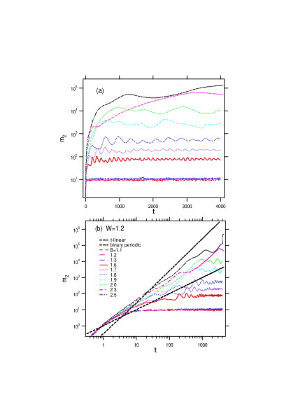
Figure 6: (Color online) (a)The second moment $m_{2}$ as a function of time for some values of $B$ at $W=1.2$. Note that the vertical axis is in the logarithmic scale. (b)The double-logarithmic plot. The ballistic motion ($m_{2}\sim t^{2}$) of the binary periodic case and diffusive lines ($m_{2}\sim t^{1}$) are shown as a reference. The results for $B=1.1,1.2,1.3$ in the bottom are almost overlapped. We set $\hbar=1$ and $\delta t=0.05$ through this paper. The system size and sample size are $N=2^{14}$ and $100$, respectively, in the numerical calculation in this section.

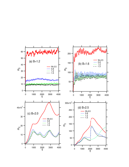
Figure 7: (Color online) The second moment $m_{2}$ as a function of time for some values of $W$ at (a)$B=1.2$, (b)$B=1.6$, (c)$B=2.0$ and (d)$B=2.5$. Note that the both axes are in the real scale.

4.2 Stationary regime ($1<B\leq 2$)

Figure 6 shows the time-dependence of MSD for the potential strength $W=1.2$ with several values of the correlation parameter $B$. First consider only the stationary regime of $B<2$. We may note that after long time the system evolves from the ballistic-like rise ($m_{2}\sim t^{2}$) to the complete localization ($m_{2}\sim t^{0}$), see the double-logarithmic plot in Fig.6(b). Furthermore, in the cases of $B=1.1,1.2,1.3$, there is no distinction in the wavepacket spreading degree. This can be easily understood, since the power spectra of the system are white-noise regardless of $B$ in the regime ($1<B<3/2$). Meanwhile, the wavepacket spreading degree increases along with the $B$ increase in the regime of $3/2<B<2$.

On the other hand, Fig.7(a)-(c) show the resulting time dependence of MSD with changing $W$. In the white noise regime, spread of the wavepacket decreases when $W$ increases, but in the region of $3/2<B<2$, the larger the value of $B$, the larger fluctuation amplitude of the MSD time dependence. This gets much more apparent when $W$ is decreasing. Furthermore, even in $B=2$ case, that is, in the nonstationary regime, the localization would seem to result from the ballistic rise, as shown in Fig.7(c).

4.3 Nonstationary regime ($B\geqq 2$)

Consider the result of quantum diffusion in the nonstationary regime. As shown in Fig.6(b) and Fig.7(d), it is complicated and its behaviour is unclear, and the results of long-time calculations with the fixed value of $W=1.2$ are shown in Fig.8(a). There, the results in the case of a binary periodic sequence ($v_{n}=(-1)^{n}$) showing complete ballistic motion ( $m_{2}\propto t^{2}$) are also shown as a reference. It seems that the MSD increases with time in the ballistic regime and localizes after passing through the intermediate spreading regime. (See the insets in Fig.8(a) and (b).) The spread is larger along with the rise in $B$, and the fluctuation becomes longer than that found in stationary regime $B<2$. Furthermore, the result in the case of the potential strength $W=0.5$ is shown in Fig.8(b). It can be noted that it dynamically localizes at $t\to\infty$, even if it is in nonstationary regime regardless of $W$. As a result, dynamical localization also occurs in these regimen investigated, so that it is in full agreement with our findings for the Lyapunov exponents and NLL shown in the previous section.

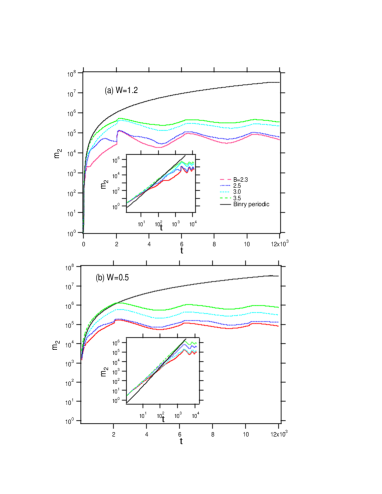
Figure 8: (Color online) The second moment $m_{2}$ as a function of time for some values of $B$ at (a)$W=1.2$ and (b)$W=0.5$. The ballistic increase ($m_{2}\sim t^{2}$) of the binary periodic system is also plotted by black bold line as a reference. Note that the vertical axis is in the logarithmic scale, and both axes of the inset in the panels (a) and (b) are in the logarithmic scale.

4.4 Scaling of the localization dynamics

The localization length becomes definite only for the perfect localization ($\sigma=0$), and infinity for $\sigma>0$, in a limit $t\to\infty$. Here, we define the DLL $\xi_{msd}$ by MSD as $m_{2}(t\to\infty)=\xi_{msd}^{2}$. Figure 9 shows the $B-$dependence of the DLL $\xi_{msd}$ numerically obtained as a time-averaged value from the data that has entered the fluctuation for a long time. It turns out to be increased sharply towards $B=2$. Even in nonstationary regime $B\geqq 2$, the localization length also increases along with the increase in $B$, but its $B$-dependence is being changed more moderately when $B>2$. Regardless of the value of $W$, the similar change in the DLL around $B\simeq 2$ can be seen in Fig.9. How does the change in the correlation of potential sequence affect the localization dynamics of the quantum system with the potential near the SNCT? The numerical results suggest that it does not change the qualitative nature of the quantum states, but we can nonetheless state that the parameter dependence experiences a change in this case.

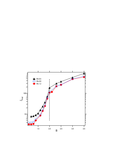
Figure 9: (Color online) Dynamical localization length $\xi_{msd}$ as a function of the correlation parameter $B$ for $W=0.5,0.8,1.2$, which are determined by ensemble-average and time-average for a period with the stable fluctuation. The $B-$dependence changes around $B\simeq 2$ from rapid increase to milder one.

As a result, in all the regions in question including the nonstationary regime the rise of the initially localized wavepacket is ballistic of $m_{2}\sim t^{2}$, and it localized at finite DLL $\xi_{msd}$ by passing through an increasing region with an index close to 2 but less than 2 ($\sigma\leq 2$), as seen in Fig.8. In this case, instead of the MSD, we introduce the scaled MSD

$$\Lambda(t)\equiv\frac{m_{2}(t)}{t^{2}}.$$ (18)

This type MSD was introduced to investigate LDT phenomena at the critical point [53]. $\Lambda=const$ if the wavepacket is extended, i.e. $m_{2}\sim t^{2}$. If this localization dynamics can be scaled only by the DLL $\xi_{msd}$, the scaling for the $t-$dependence of the scaled MSD can be expected to be as follows:

$$\Lambda(t,B,W)=F\left(\frac{t}{\xi_{msd}(B,W)}\right),$$ (19)

where the asymptotic form of the scaling function is

$$F(x)\sim\begin{cases}const&x\to 0\\ \frac{1}{x^{2}}&x\to\infty.\end{cases}$$ (20)

If the one-parameter scaling is true for the localization phenomena of the wavepacket the scaled MSD smoothly connects the asymptotic behavior in Eq.(20). Figure 10 shows $\Lambda(t)$ as a function of the scaled time $t/\xi(\alpha)$ to characterize the localization phenomenon at various $W$ and $B$ for each of the three regions. Hence, it is then clear that the case of $B<3/2$ is bridging the space from the ballistic region to the localized region even in the various combinations of $(W,B)$. These results support that the localization process from the ballistic motion ($\sim t^{2}$) to the localization ($\sim t^{0}$) in MSD of the wavepacket is scaled by a single parameter, i.e. by DLL $\xi_{msd}$.

On the other hand, as seen in the Fig.10(b), in the nonGaussian stationary regime ($3/2<B<2$), it is found that in the transient region from the ballistic motion region to the region of the localization the magnitude of the deviation becomes large although the one parameter scaling is true for sufficiently long times when localisation becomes apparent. Figure 10(c) shows the result for the non-stationary region. The deviation in this transient region becomes larger.

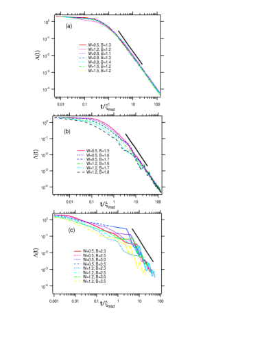
Figure 10: (Color online) Scaled MSD $\Lambda(t)$ as a function of the scaled time $t/\xi_{msd}(B,W)$ by the localization length $\xi_{msd}$. (a)White noise regime ($B<3/2$). (b)non-Gaussian stationary regime ($3/2<B<2$). (c)nonstationary regime ($B>2$). The lines with slope -2 are shown as a reference. Note that all the axes are in the logarithmic scale.

5 Summary and discussion

In summary, we numerically studied the nature of localized property in 1DDS with long-range correlation generated by modified Bernoulli map, paying attention to around $B=2$ where anomalous fluctuation of $1/f$ occurs in the potential sequence. First, we used Lyapunov exponent and the normalized localization length to investigate the localized behaviour of the wavefunctions for the band centre energy $E=0$. Lyapunov exponent linearly decreases as $B$ approaches 2 for $3/2<B<2$, and changes from the linear-decay to the exponential-decay for $B>2$. Next, we have investigated dynamical property of the initially localized wavepacket. As a result, we find that the wavepacket localizes irrespective of the stationary ($3/2<B<2$) and nonstationary regimen ($B\geqq 2$). However, it was shown that the $B-$dependence of the dynamical localization length determined by MSD changes from rapid growth to the slower one around the SNCT $B\simeq 2$. Moreover we show that the localization dynamics for $B>3/2$ deviates from the one-parameter scaling theory of the localization in the transient region from ballistic to localization.. Analysis on the dynamics of the localization is still very few in other 1DDS with long-range correlation [44].

The basic property of the quantum states is directly related to physical phenomena such as electronic conduction and transmission. In practice, we observed the physical quantities such as electronic transmission and acoustic wave localization in one-dimensional systems with sequence generated by chaotic maps [49, 50, 51, 52]. Also, real DNA chains can be described by the four symbolized sequence as ”A”, ”C”,”G”,”T, ”, and both coding and/or non-coding DNA sequences can be treated as those having the long-range correlation with the power spectrum $S(f)\sim 1/f^{\alpha}$($0.8<\alpha<1.2$) for lower $f$ [54, 55, 56, 57, 58, 59, 60]. Accordingly, it is expected that the localization-delocalization problem is strongly related to electronic conduction in the DNA chains. We expect that the present work stimulate further studies of delocalized states and the localization-delocalization transition in correlated disordered systems.

Appendix A Ensemble average

Figure 11 shows time-dependence of MSD for $B=1.8$ and $B=2.5$, which are taken ensemble average over 1000 different initial condition of the map. The global behaviour is the same as the case in text for $B=1.8$ and $B=2.5$. The fluctuation remains after the average and it is larger for the larger value of $B$. In the text, the dynamical localization length $\xi_{msd}$ based on the time-dependence is determined by taking the time average for the data in the fluctuation regime.

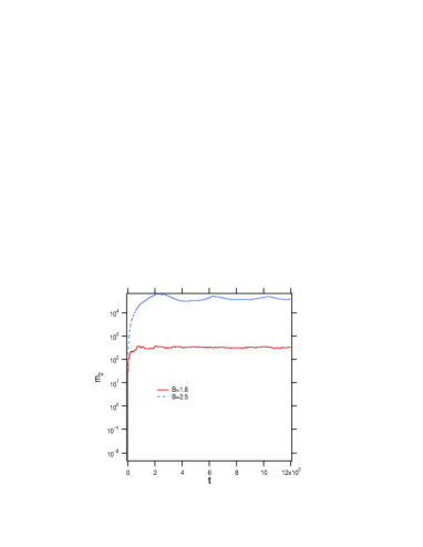
Figure 11: (Color online) MSD as a function of time for $W=1.2$ with $B=1.8,2.5$. The average is taken over 1000 different initial values of the map.

Author contribution statement

The sole author had responsibility for all parts of the manuscript.

References

- [1] K. Ishii, Prog. Theor. Phys. Suppl. 53, 77(1973).
- [2] E. Abrahams, P. W. Anderson, D. C. Licciardello, and T. V. Ramakrishnan, Rhys. Rev.Lett. 42, 673 (1979).
- [3] L.M. Lifshiz, S.A. Gredeskul and L.A. Pastur, Introduction to the theory of Disordered Systems, (Wiley, New York,1988).
- [4] F.A.B.F.de Moura, and M.L.Lyra, Phys. Rev. Lett. 81, 3735(1998).
- [5] F.M.Izrailev and A.A.Krokhin, Phys. Rev. Lett. 82, 4062(1999).
- [6] G.-P. Zhang and S.-J. Xionga, Eur. Phys. J. B 29, 491-495(2002).
- [7] H.Shima, T.Nomura and T.Nakayama, Phys. Rev. B 70, 075116(2004).
- [8] T. Kaya, Eur. Phys. J. B 55, 49(2007).
- [9] T. Kaya, Eur. Phys. J. B 67, 225 (2009).
- [10] L.Y. Gong, P.Q. Tong, and Z.C. Zhou, Eur. Phys. J. B 77, 413-417(2010).
- [11] A. Iomin, Phys. Rev. E 79, 062102(2009).
- [12] F. M. Izrailev, A. A. Krokhin, and N. M. Makarov, Phys. Rep. 512, 125 (2012).
- [13] A. Croy, P. Cain, and M. Schreiber, Eur. Phys. J. B 82, 107 (2011).
- [14] Chao-Sheng Deng, and HuiXu, Physica E 44 1473-1477(2012).
- [15] L. Gong, L. Wei, S. Zhao, and W. Cheng, Phys. Rev. E 86, 061122 (2012).
- [16] C. Albrecht and S. Wimberger, Phys. Rev. B 85, 045107 (2012).
- [17] S. Kotani, Lyapounov indices determine absolutely continuous spectra of stationary one-dimensional Schrodinger operators, Proc. Taniguchi Symp. SA. Katata, (1984), 225-248.
- [18] A. M. Garcia-Garcia, and E. Cuevas, Phys. Rev. B 79, 073104 (2009).
- [19] A. M. Garcia-Garcia, and E. Cuevas, Phys. Rev. B 82, 033412 (2010).
- [20] G.M. Petersen and N. Sandler, arXiv:1206.3370v3 [cond-mat.dis-nn].
- [21] G.M. Petersen and N. Sandler, Phys. Rev. B 87, 195443 (2013).
- [22] H.S. Yamada, Eur. Phys. J. B 88, 264 (2015); Eur. Phys. J. B 89, 158 (2016).
- [23] Shi-Jie Xiong and S. N. Evangelou, Phys. Rev. B 64, 113107(2001).
- [24] H. Yamada, M. Goda and Y. Aizawa, J. Phys.: Condens. Matter 3, 10043(1991); H.Yamada and T.Okabe, Phys. Rev. E 63, 026203(2001).
- [25] H.Yamada, Phys. Rev. B 69 014205(2004); H.Yamada, Phys. Lett. A 325 118(2004).
- [26] H. Yamada, M. Goda, Y. Aizawa, and M. Sano, J. Phys. Soc. Jpn. 61, 3050-3053 (1992).
- [27] C.R. de Oliveira and G.Q. Pellegrino, J. Phys. A 34, L239-L243 (2001).
- [28] M. O. Sales, F. A. B. F. de Moura, Physica E 45, 97-102(2012).
- [29] H. Cheraghchi, S. M. Fazeli, and K. Esfarjani, Phys. Rev. B 72, 174207(2005).
- [30] A. Esmailpour, H. Cheraghchi, P. Carpena and M. R. R. Tabar, J. Stat. Mech. P09014(2007).
- [31] E. Lazoa, E. Diezb, Phys. Lett. A 374, 3538-3545(2010).
- [32] P.Stollmann, Caught by Disorder: Bound States in Random Media, (Birkhauser, 2001).
- [33] H. N. Nazareno, J. A. Gonzalez, and Ivan F. Costa, Phys. Rev. B 57, 13583-13588(1998).
- [34] K. Sakurada, M. Goda, H. Yamada, Phys. Lett. A 280, 361-364(2001).
- [35] R. A. Pinto, M. Rodriguez, J. A. Gonzalez, and E. Medina, Phys. Rev. A 341, 101-106(2005).
- [36] A. E. B. Costa and F. A. B. F. de Moura, Int. J. Mod. Phys. C 22, 573-580(2011).
- [37] Y. Aizawa, C. Murakami and T. Kohyama, Prog. Theor. Phys. Suppl. 79, 96(1984); Y. Aizawa, Chaos, Solitons and Fractals, 11, 263(2000).
- [38] K. Tanaka and Y. Aizawa, Prog. Theor. Phys. 96, 547(1995).
- [39] T. Akimoto and Y. Aizawa, Prog. Theor. Phys. 114, 737-748(2005).
- [40] A.Crisanti, G.Paladin and A.Vulpiani, Products of random matrices in statistical physics, (Springer Series in Solid State Sciences vol. 104, Springer-Verlag 1993).
- [41] K. Takahashi and K. S. Ikeda, J. Chem. Phys. 106, 4463 (1997).
- [42] H. Yamada and K.S. Ikeda, Phys. Rev. E 59, 5214(1999); ibid, 65, 046211(2002).
- [43] D. Vollhardt and P.Wolfle: in Self-consistent theory of Anderson localization, ed. W. Hanke and Y. V. Kopaev (Elsevier Science Publishers,1992), p. 40.
- [44] B.Santos, L.P.Viana,M.L.Lyra, F.A.B.F. de Moura, Solid State Commum. 138, 1-5(2006).
- [45] P.R.Wells Jr., J. dAlbuquerque e Castro, and S.L.A. de Queiroz, Phys. Rev. B 78, 035102(2008).
- [46] Gong Long-Yan, Zhou Zi-Cong, Tong Pei-Qing and Shengmei Zhao, Physica A 390, 2977-2986(2011).
- [47] Gong Long-Yan, Tong Pei-Qing and Zhou Zi-Cong, Chinese Physics B 20, 087102 (2011).
- [48] E. Gholami and Z. M. Lashkami, Phys. Rev. E 95, 022216(2017).
- [49] A. Esmailpour, M. Esmailpour, A. Sheikhan, M. Elahi, M. R. R.Tabar, and M. Sahimi, Phys. Rev. B 78, 134206(2008).
- [50] A.E. Costa, and F.A.B.F. de Moura, J. Phys.: Condens Matter, 23, 065101(2011).
- [51] E. Diaz, A. Rodriguez, F. Domínguez-Adame and V. A. Malyshev, Europhys. Lett. 72, 1018-1024(2005).
- [52] F. Shahbazi, A. Bahraminasab, S. Mehdi Vaez Allaei, M. Sahimi, and M. Reza Rahimi Tabar, Phys. Rev. Lett. 94, 165505(2005).
- [53] R. C. Kuhn, O. Sigwarth, C. Miniatura, D. Delande, and C. A. Muller, New J. Phys. 9, 161 (2007).
- [54] C. -K.Peng, S.V.Buldyrev, A.L. Goldberger, S. Havlin, F. Sciortino, M. Simons, H.E. Stanley, Nature 356, 168(1992).
- [55] A. Rosas, E.Nogueira Jr. and J.F. Fontanari, Phys. Rev. E 66, 061906(2002). cond-mat/0209396v2.
- [56] A. Som, S. Sahoo and J. Chakrabarti, Mathematical Bioscience, 183, 49-61(2003).
- [57] Ai-Min Guo, Phys. Rev. E 75, 061915(2007).
- [58] N. Bouaynaya, and D. Schonfeld, J. Sel. Topics Signal Processing 2, 357-364 (2008).
- [59] Z. Su, T. Wu and S. Wang, Chaos, Soliton and Fractals, 40, 1750-1765(2009).
- [60] H. Yamada, Phys. Lett. A 332, 65-73(2004); H.S. Yamada and K. Iguchi, Advances in Condensed Matter Physics, 2010, Article ID 380710 (2010).