ORGB: OFFSET CORRECTION IN RGB COLOR SPACE
FOR ILLUMINATION-ROBUST IMAGE PROCESSING
Abstract
Single materials have colors which form straight lines in RGB space. However, in severe shadow cases, those lines do not intersect the origin, which is inconsistent with the description of most literature. This paper is concerned with the detection and correction of the offset between the intersection and origin. First, we analyze the reason for forming that offset via an optical imaging model. Second, we present a simple and effective way to detect and remove the offset. The resulting images, named ORGB, have almost the same appearance as the original RGB images while are more illumination-robust for color space conversion. Besides, image processing using ORGB instead of RGB is free from the interference of shadows. Finally, the proposed offset correction method is applied to road detection task, improving the performance both in quantitative and qualitative evaluations.
Index Terms— Image processing, illuminant invariance
1 Introduction
Non-uniform illumination confounds many computer vision algorithms. In particular, shadows in an image can lead segmentation, tracking, or recognition algorithms to fail. The reason lies in that the illumination-sensitive brightness and illumination-insensitive chromaticity information are mixed together in all three components of an RGB image. To remove the interference of non-uniform illumination, Color Space Conversion is often used in the pre-processing stage to separate brightness from chromaticity information. However, commonly used chromaticity spaces that claim to be illumination invariant are unstable in many natural situations, especially in the case of severe shadow. The underlying reason is related to the inaccurate description of pixel distribution characteristics. It is proved via an ideal physical model that the measured colors of homogeneous dielectric surfaces lie on a line passing through the origin of RGB space [1]. Therefore, material surfaces will form straight lines that intersect the origin. Unfortunately, it is not applicable in severe shadow cases, where Omer and Werman [2] observe that those lines are offset from the origin and do not intersect the origin if extended. The offset is also reported in [3], from which a novel reflection model is proposed. Taking the offset into consideration not only provides better image understanding but also helps improve the performance in many computer vision applications such as road detection [4] and background subtraction [5].
While existing literature either extend the existing models or adopt a new algorithm, this paper presents another perspective of dealing with the offset. Instead of changing models or algorithms, we try to change the images with the offset to that without the offset. We name that process as offset correction. Using offset correction as a pre-processing step, existing techniques including Color Space Conversion can still be applied in severe shadow cases without any modification. After offset correction, commonly used chromaticity spaces like HSV, CIELUV are illumination-robust even under severe shadow conditions. Experiments show that the offset-corrected RGB images, named ORGB, is more illumination-robust for image processing compared with the original RGB images, as shown in Fig.1. Besides, by applying the proposed offset correction into road detection task, the performance is greatly improved both in quantitative and qualitative evaluations.
2 Related Work
Most color images are captured in RGB, but this color space is rarely used for computer vision tasks. The reason is two-fold: on the one hand, the red, green and blue components are highly correlated, thus it is inefficient to process all components by analyzing nearly the same picture three times. On the other hand, since the brightness and chromaticity information are mixed together for all three components of RGB color space, they are vulnerable to the impact of illumination effects. Many computer vision algorithms start with Color Space Conversion [4, 6, 7], transforming RGB into color spaces where chromaticity components are separated from the brightness.
Although chromaticity components, e.g. hue and saturation, are illumination-robust against weak shadows, they become very unstable in severe shadow conditions [4]. The reason lies in the aforementioned offset, which undermines the pixel distribution characteristics. Under the traditional assumption, single materials have colors which form straight lines intersect the origin in RGB space. Therefore, as the intensity of the light changes, the brightness of the object changes while its color remains constant. However, due to the existence of the offset between intersection and origin, the object color do change in shadows [3, 8]. Shafer [9] attributes the color inconstancy to that the dynamic range and noise levels of cameras limit the utility of color measurements in shadows. However, that inconstancy still exists in modern cameras whose dynamic range is sufficient to capture significant information in shadows [3]. Therefore, the color inconstancy is physically present rather than be produced by cameras.
To make Color Space Conversion applicable in severe shadow cases, we need to recover the color constancy. Since the offset causes color inconstancy, the recovery of color constancy can be performed by detecting and removing that offset. To find an effective way to perform offset correction, we need to understand the reason for offset formation. In the next section, We explain it through physical modeling and experimental verification.
3 Offset Formation
To understand the formation of the offset, we take one pixel in an RGB image to analyze the imaging process. A pixel can be represented as a triplet of numbers. Denote as the measured RGB colors in that pixel. Generally, imaging devices sample the incoming light using three sensors, preferentially sensitive to long (red), medium (green), and short (blue) wavelength light respectively. The -th measured color comes from the -th sensor response, which can be modeled as
| (1) |
where is a function of wavelength characterizing how sensor responds to the captured light . For matte surfaces that do not emit light, the captured light comes from reflection as
| (2) |
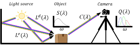
where denotes the light incident upon a surface and is its surface reflectance function. is composed of direct light and environment light . The former comes directly from the light source while the latter comes from reflections of surrounding surfaces, as shown in Fig.2. The incident light can be modeled as
| (3) |
where is a value between [0, 1] indicating how much direct light gets to the surface and is the angle between the direct lighting and the surface norm. Here is influenced by object occlusion and light attenuation. Under outdoor daylight scenes where the attenuation of sun is negligible, is 0 for umbra area, 1 for lit area and others for penumbra area.
Based on the above analysis, the overall sensor response comes from two type of light. Define the contribution of direct light to the sensor response as
| (4) |
and that of environment light as
| (5) |
then the overall sensor response is their summation:
| (6) |

(a)

(b)

(c)
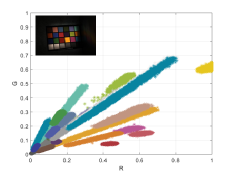
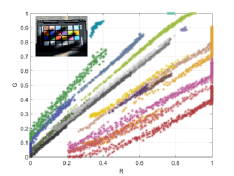
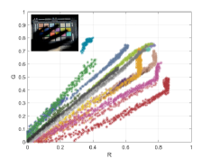
To verify the proposed model, we took pictures of a ColorChecker exposed to different light conditions. As shown in Fig.3, the ColorCheck located in image is only exposed to direct light while that in and is fully and partly occluded under outdoor daylight respectively. To observe the distribution of color lines, pixels in 24 color areas of the ColorChecker are plotted into RGB space with its corresponding color, as shown in Fig.4.
(a)
(b)
(c)
(d)
As for , of each pixel is a zero vector, and the sensor response is determined by . For the same material pixels captured by different color sensors, their responses have a proportional relationship (cf. Eq.7). For same scenario captured by one camera, that proportion is only determined by the surface reflection property, thus pixels from the same material surface will lie in one straight line passing the origin, as shown in Fig.4 (a).
| (7) |
As for , we use hand to occlude the ColorChecker, creating various illumination conditions (umbra, penumbra, and lit areas). Although pixels from the same material still distributed in a line, those lines do not intersect at origin due to the environment light, as shown in Fig.4 (b).
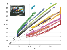
As for , the ColorChecker is entirely shrouded in shadow, thus of each pixel is a zero vector. Since and are taken in the same scene with the same camera settings, we can remove the environment light part of by subtracting . As shown in Fig.4 (c), the offset is greatly attenuated in the resulting image .
In summary, Color consistency is established only in the case of no environment light. As the presence of environment light undermines the color consistency, lines consisted of pixels from the same material do not intersect the origin. By removing the contribution from environment light, those lines will intersect at the origin again.
4 Offset Correction
In most cases, the image of corresponding environment light is not available, so we need to find another way to perform offset correction. Noticing that the straight lines in are about to converge at one point, a simple and straight-forward way is to perform a linear transform. Denote the location of that convergence point as , the offset-corrected sensor response is defined as
| (8) |
With the help of ColorCheck, can be estimated easily. As shown in Fig.4 (d), the offset of the resulting image is greatly attenuated with slight changes in appearance (a little bit brighter). The remaining problem is to find for general images without the help of ColorChecker.
After offset correction, the proportional relationship for responses of the same material pixels captured by different color sensors should be recovered. Thus, is a material dependent constant. We can use this characteristics to estimate :
| (9) |
| (10) |
| (11) |
As implied in Eq.11, there is an approximate linear relation between and among pixels from the same material. Taking advantage of this relationship, we can calculate by following steps:
-
1.
Manually select an area of interested material.
-
2.
Repeat 3-4 for each color channel ().
-
3.
Fit a straight line to approximate the relationship between and .
-
4.
Take the intercept of the line as an estimation of .
5 Experimental Results
To illustrate the practical significance of offset correction, we conducted experiments from three aspects: color space conversion, image processing and analysis.
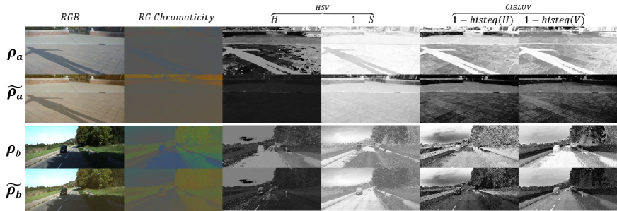
Color Space Conversion. Given the importance of color processing in both Computer Vision and Graphics, color spaces abound. While existing color spaces address a range of needs, none of them can free from the interference of severe shadows. To verify the benefit of offset correction, we perform Color Space Conversion for original RGB images and offset-corrected RGB (ORGB) images. Three common used color spaces are tested: RG Chromaticity, HSV and CIELUV. Experimental results show that the shadows in extracted color components are greatly attenuated after offset correction, as shown in Fig.5.
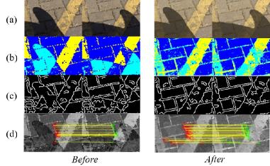
Image Processing. As color components become more illumination-robust after offset correction, color-based image processing can be improved using ORGB instead of RGB. Although there is no big difference between RGB and ORGB (c.f. Fig.1(a)), image processing results using them is quite different. The segmentation results using color components show the color constancy has been recovered after offset-correction (c.f. Fig.1(b)). Edge detection is free from the interference of severe shadow, and the object edges under shadow become clearer (cf. Fig.1(c)). As for feature match, the number of matched feature points is greatly increased (cf. Fig.1(d)).
Image Analysis. Road detection is taken as an example to demonstrate the benefit of offset correction to image analysis. As a key technique of automatic driving, road detection algorithms suffer from the shadows on road surfaces [12]. The color-based road detection framework in [4] is employed to compare the detection performances before and after offset correction. Pixel-wise measurements are used to evaluate the performance of road detection, including four measurements for quantitative evaluations (quality , detection rate , detection accuracy and effectiveness ) and one qualitative measurement called valid road result index VRI [13]. As shown in Table 1, the performance of road detection is improved after offset correction in both quantitative and qualitative measurements, especially in severe shadow cases.
| Complete dataset | |||||
|---|---|---|---|---|---|
| RGB | .80 .23 | .84 .22 | .91 .20 | .87 .20 | 81% |
| ORGB | .83 .18 | .87 .19 | .94 .14 | .89 .15 | 84% |
| Severe shadow cases | |||||
| RGB | .75 .26 | .79 .26 | .88 .24 | .82 .23 | 73% |
| ORGB | .83 .19 | .87 .20 | .93 .16 | .89 .16 | 88% |
6 Conclusions
In this paper, we present an explanation of why existing techniques cannot perform well in severe shadow cases though theoretical deduction and experimental verification. We attribute the reason to the offset caused by environment light, which is ignored in many literature. Instead of modifying models or algorithms, we proposed an image pre-processing method to remove the offset. Experimental results show that offset correction can improve the performance of color space conversion in severe shadow cases. Besides, the proposed method can be applied to image processing and analysis via existing models or algorithms without any modification. To encourage future works, we make the source code open, as well as related materials. More testing results can be found on our project website: https://baidut.github.io/ORGB/.
References
- [1] Glenn Healey, “Segmenting images using normalized color,” Systems, Man and Cybernetics, IEEE Transactions on, vol. 22, no. 1, pp. 64–73, 1992.
- [2] Ido Omer and Michael Werman, “Color lines: Image specific color representation,” in Computer Vision and Pattern Recognition, 2004. CVPR 2004. Proceedings of the 2004 IEEE Computer Society Conference on. IEEE, 2004, vol. 2, pp. II–946.
- [3] Bruce A Maxwell, Richard M Friedhoff, and Casey A Smith, “A bi-illuminant dichromatic reflection model for understanding images,” in Computer Vision and Pattern Recognition, 2008. CVPR 2008. IEEE Conference on. IEEE, 2008, pp. 1–8.
- [4] Z. Ying, G. Li, X. Zang, R. Wang, and W. Wang, “A novel shadow-free feature extractor for real-time road detection,” in Proceedings of the 24rd ACM international conference on Multimedia. ACM, 2016, (in press).
- [5] Jia-Bin Huang and Chu-Song Chen, “Moving cast shadow detection using physics-based features,” in Computer Vision and Pattern Recognition, 2009. CVPR 2009. IEEE Conference on. IEEE, 2009, pp. 2310–2317.
- [6] Z. Ying and G. Li, “Robust lane marking detection using boundary-based inverse perspective mapping,” in 2016 IEEE International Conference on Acoustics, Speech and Signal Processing (ICASSP), March 2016, pp. 1921–1925.
- [7] Z. Ying, G. Li, and G. Tan, “An illumination-robust approach for feature-based road detection,” in 2015 IEEE International Symposium on Multimedia (ISM), Dec 2015, pp. 278–281.
- [8] Graham D Finlayson, Steven D Hordley, Cheng Lu, and Mark S Drew, “On the removal of shadows from images,” Pattern Analysis and Machine Intelligence, IEEE Transactions on, vol. 28, no. 1, pp. 59–68, 2006.
- [9] Steven A Shafer, “Using color to separate reflection components,” Color Research & Application, vol. 10, no. 4, pp. 210–218, 1985.
- [10] Han Gong and DP Cosker, “Interactive shadow removal and ground truth for variable scene categories,” in BMVC 2014-Proceedings of the British Machine Vision Conference 2014. University of Bath, 2014.
- [11] Joerg Fritsch, Tobias Kuhnl, and Andreas Geiger, “A new performance measure and evaluation benchmark for road detection algorithms,” in Intelligent Transportation Systems-(ITSC), 2013 16th International IEEE Conference on. IEEE, 2013, pp. 1693–1700.
- [12] Aharon Bar Hillel, Ronen Lerner, Dan Levi, and Guy Raz, “Recent progress in road and lane detection: a survey,” Machine Vision and Applications, vol. 25, no. 3, pp. 727–745, 2014.
- [13] Jose M Álvarez, Theo Gevers, and Antonio M Lopez, “3d scene priors for road detection,” in Computer Vision and Pattern Recognition (CVPR), 2010 IEEE Conference on. IEEE, 2010, pp. 57–64.
- [14] T. Veit, J.-P. Tarel, P. Nicolle, and P. Charbonnier, “Evaluation of road marking feature extraction,” in Intelligent Transportation Systems, 2008. ITSC 2008. 11th International IEEE Conference on, Oct 2008, pp. 174–181.