1 Introduction

Uncertainty quantification (UQ) examines the dependence of outputs on vague input parameters in mathematical models, see [21]. Often the uncertain parameters are replaced by random variables or random processes, resulting in a stochastic problem. We consider dynamical systems consisting of ordinary differential equations (ODEs) with random parameters. The state variables can be expanded into a series of orthogonal basis functions, where often polynomials are applied (polynomial chaos), see [1, 4, 22]. Stochastic Galerkin methods or stochastic collocation techniques yield numerical solutions of unknown coefficient functions. We focus on the stochastic Galerkin approach, see [2, 11, 13], in this paper.

Sonday et al. [19] analyzed the spectrum of a Jacobian matrix of a Galerkin-projected (nonlinear) system of ODEs. The results indicate that a preservation of stability is not guaranteed in the Galerkin projection even if the original system is asymptotically stable. Even though a loss of stability happens rather seldom, this change in stability leads to unexpected and erroneous results. Therefore, we derive a technique, which guarantees the asymptotic stability in the Galerkin-projected system provided that the original system is asymptotically stable.

Prajna [10] designed an approach to preserve stability in a projection-based model order reduction of a (nonlinear) system of ODEs. Therein, a dynamical system is reduced to a smaller dynamical system. We apply a similar strategy in the stochastic Galerkin method, where a random dynamical system is projected to a larger deterministic dynamical system. The stability-preserving technique employs a basis transformation of the original parameter-dependent system, where the transformation matrix is derived from the solution of a Lyapunov equation.

We construct and investigate this transformation for linear dynamical systems in detail. A proof of the stability preservation is given for the stabilized stochastic Galerkin method. Furthermore, we consider the asymptotic stability of stationary solutions (equilibria) for autonomous nonlinear dynamical systems. In [12], existence and convergence of stationary solutions was analyzed in the stochastic Galerkin-projected systems. The Galerkin system exhibits equilibria, which yield approximations to the random-dependent equilibria of the original system. The approximations converge in mean square to the exact equilibria. Now we apply the basis transformation to guarantee the stability of the stationary solutions in the stochastic Galerkin-projected system.

The paper is organized as follows. The stochastic Galerkin approach is described for the linear case in Section 2. The stability-preserving projection is derived and analyzed in Section 3. An analogous stabilization is specified for the nonlinear case in Section 4. Finally, Section 5 includes numerical results for both a linear and a nonlinear test example.

2 Problem definition

The class of linear problems under investigation is described in this section.

2.1 Linear dynamical systems and stability

We consider a linear dynamical system of the form

$$\dot{x}(t,p)=A(p)x(t,p)+s(t,p),$$ (1)

where the matrix $A:\Pi\rightarrow\mathbbm{R}^{n\times n}$ and the vector $s:[0,\infty)\times\Pi\rightarrow\mathbbm{R}^{n}$ depend on parameters $p\in\Pi$ for some subset $\Pi\subseteq\mathbbm{R}^{q}$. Consequently, the state variables $x:[0,\infty)\times\Pi\rightarrow\mathbbm{R}^{n}$ are also parameter-dependent. Initial value problems are determined by

$$x(0,p)=x_{0}(p)$$

with a given function $x_{0}:\Pi\rightarrow\mathbbm{R}^{n}$. Since we are investigating stability properties, let, without loss of generality, $s\equiv 0$ in the system (1).

To analyze the stability, we recall some general properties of matrices.

Definition 1

Let $A\in\mathbbm{R}^{n\times n}$ and $\lambda_{1},\ldots,\lambda_{n}\in\mathbbm{C}$ be its eigenvalues. The spectral abscissa of the matrix $A$ reads as

$$\alpha(A):=\max\left\{{\rm Re}(\lambda_{1}),\ldots,{\rm Re}(\lambda_{n})\right\}.$$

$A$ is called a stable matrix, if it holds that $\alpha(A)<0$.

A linear dynamical system $\dot{x}=Ax$ is asymptotically stable if and only if the included matrix $A$ is stable. We assume that the matrices $A(p)$ in the system (1) are stable for all $p\in\Pi$ in the following.

2.2 Stochastic modeling and orthogonal expansions

Now we assume that the parameters in equation (1) are affected by uncertainties. In uncertainty quantification, the parameters are replaced by independent random variables $p:\Omega\rightarrow\Pi$ on some probability space $(\Omega,\mathscr{A},\mu)$. Let a joint probability density function $\rho:\Pi\rightarrow\mathbbm{R}$ be given. Without loss of generality, we assume $\Pi={\rm supp}(\rho)$, because the parameter space $\Pi$ can be restricted to the support of $\rho$ otherwise. For a measurable function $f:\Pi\rightarrow\mathbbm{R}$, the expected value reads as

$$\mathbb{E}\left[f\right]:=\int_{\Omega}f(p(\omega))\;\mbox{d}\mu(\omega)=\int_{\Pi}f(p)\rho(p)\;\mbox{d}p$$ (2)

provided that the integral exists. The Hilbert space

$$\mathscr{L}^{2}(\Pi,\rho):=\left\{f:\Pi\rightarrow\mathbbm{R}\;:\;f\;\mbox{measurable and}\;\mathbb{E}\left[f^{2}\right]<\infty\right\}$$

is equipped with the inner product

$$\left\langle f,g\right\rangle\;=\int_{\Pi}f(p)g(p)\rho(p)\;\mbox{d}p\qquad\mbox{for}\;\;f,g\in\mathscr{L}^{2}(\Pi,\rho).$$

Let a complete orthonormal system $(\Phi_{i})_{i\in\mathbbm{N}}$ be given. Thus the basis functions $\Phi_{i}:\Pi\rightarrow\mathbbm{R}$ satisfy

$$\left\langle\Phi_{i},\Phi_{j}\right\rangle\;=\left\{\begin{array}[]{ll}0&\mbox{for}\;\;i\neq j,\\ 1&\mbox{for}\;\;i=j.\\ \end{array}\right.$$ (3)

Assuming $x_{k}(t,\cdot)\in\mathscr{L}^{2}(\Pi,\rho)$ for each component $k=1,\ldots,n$ and each time point $t$, the state variables of the system (1) can be expanded into a series

$$x(t,p)=\sum_{i=1}^{\infty}v_{i}(t)\Phi_{i}(p).$$ (4)

The coefficient functions $v_{i}:[0,\infty)\rightarrow\mathbbm{R}^{n}$ are defined by

$$v_{i,k}=\;\left\langle x_{k}(t,\cdot),\Phi_{i}(\cdot)\right\rangle\qquad\mbox{for}\;\;k=1,\ldots,n.$$ (5)

The series (4) converges in the norm of $\mathscr{L}^{2}(\Pi,\rho)$ point-wise for each $t$. Often polynomials are used as basis functions following the concepts of the generalized polynomial chaos (gPC). More details can be found in [22].

2.3 Galerkin projection of linear dynamical systems

Stochastic Galerkin methods and stochastic collocation techniques yield approximations of the coefficient functions (5) in the expansion (4), see [2, 11, 13, 15]. We apply the stochastic Galerkin approach, where Equation (1) is projected onto a finite subset $\{\Phi_{1},\ldots,\Phi_{m}\}$ of basis functions. The stochastic process (4) is approximated by a truncated expansion

$$\hat{x}^{(m)}(t,p)=\sum_{i=1}^{m}\hat{v}_{i}(t)\Phi_{i}(p).$$

The Galerkin projection of the dynamical system (1), neglecting the term $s$, results in the larger linear dynamical system

$$\dot{\hat{v}}(t)=\hat{A}\hat{v}(t),$$ (6)

whose solution $\hat{v}=(\hat{v}_{1}^{\top},\ldots,\hat{v}_{m}^{\top})^{\top}$ represents an approximation of the exact coefficient functions (5). The matrix $\hat{A}\in\mathbbm{R}^{mn\times mn}$ is defined by its minors $\hat{A}_{ij}\in\mathbbm{R}^{n\times n}$ with

$$\hat{A}_{ij}=\mathbb{E}\left[A\Phi_{i}\Phi_{j}\right]\qquad\mbox{for}\;\;i,j=1,\ldots,m$$

using the matrix $A$ from (1). Therein, the expected value, see (2), is applied componentwise. If the matrix $A(p)$ is symmetric for almost all $p$, then the matrix $\hat{A}$ is also symmetric. Otherwise, the matrix $\hat{A}$ is unsymmetric, which is the case in many situations.

The convergence properties of the stochastic Galerkin approach are not investigated in this paper. Alternatively, we examine the stability properties. The analysis in [19] shows that the matrix $\hat{A}$ may be unstable even though $A(p)$ is stable for strictly all $p$ with respect to Definition 1. Yet the stability is guaranteed in the case of normal matrices $A(p)$ for almost all $p$. Even though stability can be lost for non-normal matrices, the stochastic Galerkin method is still convergent on compact time intervals under usual assumptions.

2.4 Basis transformations

We consider a transformation of the linear dynamical system (1), with $s\equiv 0$, to an equivalent system

$$\dot{y}(t,p)=B(p)y(t,p)$$ (7)

with $y(t,p):=T(p)x(t,p)$ and transformation matrices $T:\Pi\rightarrow\mathbbm{R}^{n\times n}$ being point-wise non-singular. It holds that

$$B(p)=T(p)A(p)T(p)^{-1}$$ (8)

for each $p\in\Pi$. The operation (8) represents a similarity transformation, i.e., the spectra of the matrices $A(p)$ and $B(p)$ coincide.

If the stochastic Galerkin system (6) is unstable, then our aim is to identify a basis transformation given by a matrix $T:\Pi\rightarrow\mathbbm{R}^{n\times n}$ such that the Galerkin projection of the dynamical system (7) yields a stable system. The following properties of the basis transformation are required:

1. $T$ has to be non-constant in the variable $p$. The Galerkin approach is invariant with respect to constant basis transformations and thus the stability properties cannot be changed.

2. If $A\in\mathscr{C}^{\ell}(\Pi)^{n\times n}$, then $T\in\mathscr{C}^{\ell}(\Pi)^{n\times n}$ is required to guarantee $B\in\mathscr{C}^{\ell}(\Pi)^{n\times n}$ and thus $y(t,\cdot)\in\mathscr{C}^{\ell}(\Pi)^{n}$ for each $t$. The convergence rate of orthogonal (gPC) expansions depends on the order of differentiability in the random-dependent functions, see [1, p. 154] and [22, p. 33].

3 Stability preservation

We derive a concept to guarantee the stability of the dynamical system obtained by the stochastic Galerkin projection.

3.1 General results

In this subsection, a constant matrix $A\in\mathbbm{R}^{n\times n}$ is considered. If the matrix $A$ is unsymmetric, then the following definition allows for further investigations.

Definition 2

The symmetric part of a matrix $A\in\mathbbm{R}^{n\times n}$ reads as

$$A_{\rm sym}:=\textstyle\frac{1}{2}(A+A^{\top}).$$

The symmetric part of $A$ is negative definite if and only if $A+A^{\top}$ is negative definite. We will apply the following well-known property later.

Lemma 1

If the symmetric part of $A\in\mathbbm{R}^{n\times n}$ is negative definite, then $A$ is a stable matrix.

Proof:

The spectral abscissa is bounded by $\alpha(A)\leq\mu(A)$ for an arbitrary logarithmic norm $\mu$. The logarithmic norm associated with the Euclidean vector norm reads as $\mu(A)=\alpha(A_{\rm sym})$, see [8, p. 61]. The negative definiteness of the symmetric part implies $\alpha(A_{\rm sym})<0$. It follows that $\alpha(A)<0$. $\Box$

Assuming that the symmetric part of a given matrix $A$ is not negative definite, we construct a transformation matrix $T$ such that the symmetric part of the similarity-transformed matrix $B=TAT^{-1}$ becomes negative definite.

Theorem 1

Let $A\in\mathbbm{R}^{n\times n}$ be a stable matrix and $Q\in\mathbbm{R}^{n\times n}$ be a symmetric positive definite matrix. The Lyapunov equation

$$A^{\top}M+MA+Q=0$$ (9)

has a unique symmetric positive definite solution $M\in\mathbbm{R}^{n\times n}$. For a symmetric decomposition $M=LL^{\top}$ with $L\in\mathbbm{R}^{n\times n}$, a similarity transformation yields the matrix

$$B:=L^{\top}AL^{-\top},$$ (10)

which features a negative definite symmetric part.

Proof:

The stability of the matrix $A$ guarantees existence and uniqueness of a solution $M$ for the Lyapunov equation (9), see [7, p. 303]. The symmetric matrix $M$ is positive definite, because $Q$ is positive definite. The symmetric part of the matrix (10) becomes (neglecting the factor $\frac{1}{2}$)

$$\begin{array}[]{rcl}B+B^{\top}&=&L^{\top}AL^{-\top}+L^{-1}A^{\top}L\\[4.30554pt] &=&L^{-1}(MA+A^{\top}M)L^{-\top}\\[4.30554pt] &=&-L^{-1}QL^{-\top}.\\ \end{array}$$

The matrix $-L^{-1}QL^{-\top}$ is negative definite due to the positive-definiteness of $Q$, since

$$z^{\top}(-L^{-1}QL^{-\top})z=-(L^{-\top}z)^{\top}Q(L^{-\top}z)<0$$

for all $z\in\mathbbm{R}^{n}\backslash\{0\}$. $\Box$

The proof of Theorem 1 follows mainly the steps in [10, Thm. 5]. However, a symmetric decomposition $M=M^{\frac{1}{2}}M^{\frac{1}{2}}$ is assumed in [10], which requires the computation of all eigenvalues and eigenvectors. Furthermore, this decomposition is not unique in the case of multiple eigenvalues. Theorem 1 holds true for arbitrary symmetric decompositions of $M$. In particular, we may apply the Cholesky factorization $M=LL^{\top}$, where $L$ becomes a unique lower triangular matrix with strictly positive diagonal elements, see [20, p. 204]. Efficient algorithms are available to compute the Cholesky factor without first finding $M$, see [7]. More details on Lyapunov equations can be found in [5], for example.

3.2 Stability-preserving transformation

The linear dynamical system (1) is assumed to involve stable matrices $A(p)$ for all $p\in\Pi$. In view of (9), we use the parameter-dependent Lyapunov equations

$$A(p)^{\top}M(p)+M(p)A(p)+Q(p)=0\qquad\mbox{for each}\;\;p\in\Pi.$$ (11)

Let the matrices $Q(p)$ be symmetric positive definite for all $p$. Constant choices $Q(p)\equiv Q_{0}$ are admissible. Consequently, the system (11) has a unique symmetric positive definite solution $M(p)$ for each $p$. We require a symmetric decomposition of $M(p)$ for each $p$. Concerning the smoothness, we demonstrate a property of the Cholesky factorization. The proof follows the steps in [16, p. 295], where the continuity of this decomposition is shown.

Lemma 2

If $A\in\mathscr{C}^{\ell}(\Pi)^{n\times n}$ and $A(p)$ is symmetric as well as positive definite for all $p\in\Pi$, then the Cholesky decomposition $A=LL^{\top}$ satisfies $L\in\mathscr{C}^{\ell}(\Pi)^{n\times n}$.

Proof:

We use induction with respect to $n$. For $n=1$, we obtain $A(p)=(\alpha(p))$ with $\alpha(p)>0$ for all $p$. It follows that $L(p)=(\sqrt{\alpha(p)})$. Thus $L\in\mathscr{C}^{\ell}(\Pi)^{1\times 1}$ is satisfied, because the square root is differentiable to arbitrary order for positive real numbers. Now let the assumption be valid for $n-1$. We partition a matrix $A(p)\in\mathbbm{R}^{n\times n}$ and its Cholesky decomposition into

$$A(p)=\begin{pmatrix}\alpha(p)&r(p)\\ r(p)^{\top}&\bar{A}(p)\\ \end{pmatrix}\quad\mbox{and}\quad L(p)=\begin{pmatrix}\beta(p)&0\\ s(p)^{\top}&B(p)\\ \end{pmatrix}.$$

Since $A(p)$ is positive definite, it holds that $\alpha(p)>0$ for all $p$. We obtain $\beta(p)=\sqrt{\alpha(p)}$, $s(p)=\frac{r(p)}{\sqrt{\alpha(p)}}$ and $B(p)B(p)^{\top}=\bar{A}(p)-\frac{r(p)^{\top}r(p)}{\alpha(p)}=:F(p)$. The mapping $p\mapsto F(p)$ is in $\mathscr{C}^{\ell}(\Pi)^{n\times n}$ due to $A\in\mathscr{C}^{\ell}(\Pi)^{n\times n}$. Hence the mapping $p\mapsto B(p)$ is in $\mathscr{C}^{\ell}(\Pi)^{n\times n}$ by the assumption in the induction. Note that the operations used to compute $\beta$ and $s$ are differentiable to arbitrary orders. $\Box$

The following result guarantees the preservation of smoothness.

Lemma 3

If $A,Q\in\mathscr{C}^{\ell}(\Pi)^{n\times n}$, then it follows that $B\in\mathscr{C}^{\ell}(\Pi)^{n\times n}$ for the transformed matrix (8) using the Cholesky factorization of the solutions from the Lyapunov equations (11).

Proof:

Each Lyapunov equation (11) represents a larger linear system of algebraic equations. Assuming $A,Q\in\mathscr{C}^{\ell}(\Pi)^{n\times n}$, Cramer’s rule implies that the entries in the solution $M$ are also in $\mathscr{C}^{\ell}(\Pi)$. Lemma 2 yields the differentiability $L\in\mathscr{C}^{\ell}(\Pi)^{n\times n}$. The inverse matrix inherits the smoothness $L^{-1}\in\mathscr{C}^{\ell}(\Pi)^{n\times n}$, because it holds that $L^{-1}(p)=\frac{{\rm adj}(L(p))}{\det(L(p))}$ for each $p$ with the adjoint matrix. Now formula (8) demonstrates that $B\in\mathscr{C}^{\ell}(\Pi)^{n\times n}$. $\Box$

In particular, Lemma 3 is valid in the case of continuous functions ($\ell=0$). Furthermore, just measurable matrix-valued functions $A,Q$ imply measurable matrix-valued functions $M,L$.

If the entries of $A$ and $Q$ are polynomials in the variable $p$, then the entries of $M$ become rational functions. However, the entries of the factor $L$ in a symmetric decomposition are not rational functions in general, because a square root is typically applied somewhere. Consequently, the transformed matrix (10) does not represent a rational function in general.

We transform the original dynamical system (1) into (7) using the transformation matrix $T(p):=L(p)^{\top}$ for an arbitrary symmetric decomposition $M(p)=L(p)L(p)^{\top}$. The main result is formulated now.

Theorem 2

Let $A,Q:\Pi\rightarrow\mathbbm{R}^{n\times n}$ be measurable functions with $A(p)$ stable and $Q(p)$ symmetric as well as positive definite for almost all $p\in\Pi$. The Lyapunov equation (11) yields a unique solution $M(p)$ for almost all $p$. A symmetric decomposition $M(p)=L(p)L(p)^{\top}$ is considered for almost all $p$. Furthermore, let $A\in\mathscr{L}^{q_{1}}(\Pi,\rho)^{n\times n}$, $L\in\mathscr{L}^{q_{2}}(\Pi,\rho)^{n\times n}$, $L^{-1}\in\mathscr{L}^{q_{3}}(\Pi,\rho)^{n\times n}$ with $q_{k}\in[1,\infty]$ for $k=1,2,3$ and $\frac{1}{2}=\frac{1}{q_{1}}+\frac{1}{q_{2}}+\frac{1}{q_{3}}$. Using $T(p):=L(p)^{\top}$, the Galerkin projection of the transformed system (7) with the matrix (8) produces an asymptotically stable linear dynamical system.

Proof:

The generalized Hölder inequality guarantees $B=TAT^{-1}\in\mathscr{L}^{2}(\Pi,\rho)^{n\times n}$ due to the regularity assumptions for $A,L,L^{-1}$. The stochastic Galerkin approach applied to the transformed system (7) including the matrix (8) yields a dynamical system $\dot{\hat{v}}=\hat{B}\hat{v}$ with the matrix $\hat{B}\in\mathbbm{R}^{mn\times mn}$. The minors $\hat{B}_{ij}\in\mathbbm{R}^{n\times n}$ read as $\hat{B}_{ij}=\mathbb{E}\left[B\Phi_{i}\Phi_{j}\right]$ for $i,j=1,\ldots,m$. We investigate the symmetric part of the matrix $\hat{B}$. The minors of the symmetric part $\hat{B}+\hat{B}^{\top}$ become

$$\hat{B}_{ij}+(\hat{B}_{ji})^{\top}=\mathbb{E}\left[B\Phi_{i}\Phi_{j}\right]+\mathbb{E}\left[B^{\top}\Phi_{j}\Phi_{i}\right]=\mathbb{E}\left[(B+B^{\top})\Phi_{i}\Phi_{j}\right].$$

Given the transformation (8) with $T(p)=L(p)^{\top}$, Theorem 1 shows that the symmetric part, $B(p)+B(p)^{\top}$, of the matrix (10) is negative definite for almost all $p$. Let $z=(z_{1}^{\top},\ldots,z_{m}^{\top})^{\top}\in\mathbbm{R}^{mn}$ with $z_{1},\ldots,z_{m}\in\mathbbm{R}^{n}$. It follows that

$$\begin{array}[]{rcl}z^{\top}(\hat{B}+\hat{B}^{\top})z&=&\displaystyle\sum_{i,j=1}^{m}z_{i}^{\top}\left(\hat{B}_{ij}+\hat{B}_{ji}^{\top}\right)z_{j}\;\;=\;\;\mathbb{E}\left[\sum_{i,j=1}^{m}z_{i}^{\top}(B+B^{\top})z_{j}\Phi_{i}\Phi_{j}\right]\\ &=&\displaystyle\mathbb{E}\left[\left(\sum_{i=1}^{m}z_{i}\Phi_{i}\right)^{\top}(B+B^{\top})\left(\sum_{j=1}^{m}z_{j}\Phi_{j}\right)\right]\;\;\leq\;\;0.\\ \end{array}$$

Since the basis functions are linearly independent, it holds that

$$\tilde{z}:=\sum_{i=1}^{m}z_{i}\Phi_{i}\in\mathscr{L}^{2}(\Pi,\rho)\backslash\{0\}\qquad\mbox{for}\;\;z\neq 0.$$

Assuming $z\neq 0$, the function $\tilde{z}$ is non-zero on a subset $U\subset\Pi$ with $\mu(U)>0$ for the probability measure $\mu$. It follows that the above expected value becomes strictly negative. Hence the symmetric part $\hat{B}+\hat{B}^{\top}$ is negative definite. Lemma 1 shows that $\hat{B}$ is a stable matrix. Consequently, the dynamical system $\dot{\hat{v}}=\hat{B}\hat{v}$ is asymptotically stable. $\Box$

The above result is independent of the choice of orthogonal basis functions. Moreover, the system of basis functions is not required to be complete. Note that any symmetric decomposition can be used satisfying the suppositions in Theorem 2.

Concerning the regularity assumptions, the choice $q_{1}=q_{2}=q_{3}=6$ is admissible, for example. Furthermore, $q_{i}=\infty$ can be chosen for one particular $i$, with $\frac{1}{q_{i}}=0$. It holds that $\mathscr{L}^{\infty}(\Pi,\rho)\subset\mathscr{L}^{q}(\Pi,\rho)$ for any $q\in[1,\infty)$. The regularity properties of the matrix-valued functions $L,L^{-1}$ depend on the functions $A$ and $Q$. We outline sufficient conditions for the regularity assumptions of Theorem 2 in two cases, where the Cholesky decomposition is considered:

• Compact domain $\Pi$ (e.g., uniform distribution, beta distribution, etc): if $A,Q\in\mathscr{C}^{0}(\Pi)^{n\times n}$, then $L,L^{-1}\in\mathscr{C}^{0}(\Pi)^{n\times n}$ as shown in the proof of Lemma 3. Compact domains imply $\mathscr{C}^{0}(\Pi)^{n\times n}\subset\mathscr{L}^{\infty}(\Pi,\rho)^{n\times n}$. Hence continuity of $A$ and $Q$ is sufficient.

• Unbounded domain $\Pi$ and exponentially decaying probability density function $\rho$ for $p\rightarrow\infty$ (e.g., Gaussian distribution, gamma distribution, etc.): if the components of $A,Q$ are (multivariate) polynomials in $p$, then all entries of both $M$ and $M^{-1}$ are rational functions in $p$. Consequently, these entries exhibit at most polynomial growth for $p\rightarrow\infty$. The matrices $L,L^{-1}$ inherit this behavior. Since $\rho$ decreases exponentially, we obtain $A,L,L^{-1}\in\mathscr{L}^{q}(\Pi,\rho)$ for any $q\in[1,\infty)$.

3.3 Numerical computation of Galerkin projection

In Theorem 2, the transformation matrix $T(p)=L(p)^{\top}$ depends on the parameters $p\in\Pi$. The solution of the Lyapunov equations (11) and its symmetric decomposition can be computed analytically only for simple systems. We require numerical methods for general systems.

Table 1: Probability distributions and Gaussian quadrature methods.

probability distribution	quadrature rule
uniform	Gauss-Legendre
Gaussian	Gauss-Hermite
beta	Gauss-Jacobi
gamma	Gauss-Laguerre

We compute the Galerkin projection of the transformed matrix (8) by a quadrature rule for the weighted integrals (2), where the probability density is the weight function. A quadrature scheme is defined by its nodes $\{p^{(1)},\ldots,p^{(k)}\}\subset\Pi$ and weights $\{w_{1},\ldots,w_{k}\}\subset\mathbbm{R}$. For example, Gaussian quadrature can be applied for a single random variable, see [20, p. 171]. Each traditional probability distribution induces a weighted integral (2) and an associated Gaussian quadrature rule. Table 1 illustrates the most important cases. Tensor product rules of Gaussian quadrature can be used for multiple random variables ($\Pi\subseteq\mathbbm{R}^{q}$), provided that the number $q$ is not too large.

Using a general quadrature method, the approximation $\tilde{B}\in\mathbbm{R}^{mn\times mn}$ of $\hat{B}\in\mathbbm{R}^{mn\times mn}$ is given by

$$\hat{B}_{ij}=\mathbb{E}\left[B\Phi_{i}\Phi_{j}\right]\approx\tilde{B}_{ij}:=\sum_{r=1}^{k}w_{r}B(p^{(r)})\Phi_{i}(p^{(r)})\Phi_{j}(p^{(r)})$$ (12)

for $i,j=1,\ldots,m$. The exact matrix $\hat{B}+\hat{B}^{\top}$ is negative definite due to Theorem 2. Given a sufficiently accurate quadrature rule, the approximation $\tilde{B}+\tilde{B}^{\top}$ is negative definite as well, because the eigenvalues of a matrix depend continuously on its entries. Hence the linear dynamical system $\dot{\tilde{v}}=\tilde{B}\tilde{v}$ inherits the asymptotic stability.

We show a sufficient condition with respect to the magnitude of the quadrature error.

Theorem 3

Let $\hat{B},\tilde{B},\Delta B\in\mathbbm{R}^{mn\times mn}$ and $\hat{B}=\tilde{B}+\Delta B$. If $\hat{B}+\hat{B}^{\top}$ is negative definite and

$$\left\|\Delta B\right\|_{2}<\textstyle{\frac{1}{2}}|\alpha(\hat{B}+\hat{B}^{\top})|$$

with the spectral (matrix) norm $\|\cdot\|_{2}$ and the spectral abscissa $\alpha$, then $\tilde{B}+\tilde{B}^{\top}$ is also negative definite. Hence the matrix $\tilde{B}$ is stable.

Proof:

The eigenvalues of $\hat{B}+\hat{B}^{\top}$ are $\lambda_{1}\leq\lambda_{2}\leq\cdots\leq\lambda_{mn}<0$. It holds that $\alpha(\hat{B}+\hat{B}^{\top})=\lambda_{mn}$. The matrix $\hat{B}+\hat{B}^{\top}$ is symmetric and thus diagonalizable. An orthonormal basis of eigenvectors exists, which forms a square matrix of condition number one with respect to the spectral norm. Let $\mu\in\mathbbm{R}$ be an eigenvalue of the symmetric matrix $\tilde{B}+\tilde{B}^{\top}$. The Theorem of Bauer-Fike, see [6, p. 357], implies

$$\min_{j=1,\ldots,mn}|\mu-\lambda_{i}|\leq\left\|\Delta B+\Delta B^{\top}\right\|_{2}\leq 2\|\Delta B\|_{2}<|\lambda_{mn}|.$$

The minimum is $|\mu-\lambda_{\ell}|$ with some $\ell\in\{1,\ldots,mn\}$. It follows that $|\mu-\lambda_{\ell}|<-\lambda_{mn}$ and $\mu<-\lambda_{mn}+\lambda_{\ell}\leq 0$. Thus $\tilde{B}+\tilde{B}^{\top}$ is negative definite. Lemma 1 shows that $\tilde{B}$ is a stable matrix. $\Box$

In Theorem 3, the perturbation $\Delta B$ consists of the quadrature errors concerning (12). If the quadrature rule is inaccurate, then the matrix $\tilde{B}+\tilde{B}^{\top}$ may not be negative definite. Consequently, the stability can be lost in the approximate Galerkin projection.

The evaluation of the formula (12) for all $i,j=1,\ldots,m$ requires mainly to calculate $k$ transformed matrices (8). The effort for the evaluation of the basis polynomials is negligible. We have to solve the Lyapunov equations (11) for $k$ different realizations of the random parameters. In addition, we have to compute a symmetric decomposition for each $M(p^{(r)})$ with $r=1,\ldots,k$. Based on the algorithm of Bartels and Stewart [3], numerical techniques were derived to compute the Cholesky factor without having to compute $M$ first, see [7, 9]. These direct linear algebra methods exhibit a computational effort of $O(n^{3})$ operations. Thus our total computational work becomes $O(kn^{3})$. This effort is acceptable in the case of moderate dimensions $n$. Typically, we need larger numbers of nodes for polynomials of higher degrees. For example, with polynomials $\Phi_{i}$ of degree $i-1$ in a single random variable ($q=1$), the approximation (12) requires a Gaussian quadrature with $k\geq m+1$ nodes. If the matrix-valued function $B$ is close to a polynomial of degree $d$, then $k\approx m+\frac{d}{2}$ nodes are sufficient.

For comparison, an $LU$-decomposition of a dense Galerkin-projected matrix $\hat{A}$ or $\hat{B}$ costs $O(m^{3}n^{3})$ operations, which is required in implicit time integrators. The matrices are typically sparse for high dimensions $n$, where iterative methods have to be used for solving Lyapunov equations. Furthermore, there is some potential to reduce the computational effort by numerical methods for parameter-dependent Lyapunov equations, cf. [18].

4 Nonlinear dynamical systems

We derive a stabilization for nonlinear dynamical systems now.

4.1 Stationary solutions

Let a nonlinear autonomous dynamical system

$$\dot{x}(t,p)=f(x(t,p),p)$$ (13)

be given, including a sufficiently smooth function $f:D\times\Pi\rightarrow\mathbbm{R}^{n}$ ($D\subseteq\mathbbm{R}^{n}$). We assume that a family of asymptotically stable stationary solutions $x^{*}:\Pi\rightarrow\mathbbm{R}^{n}$ exists, i.e.,

$$f(x^{*}(p),p)=0\qquad\mbox{for all}\;\;p\in\Pi.$$ (14)

The asymptotic stability means that the Jacobian matrix $\left.\textstyle\frac{\partial f}{\partial x}\right|_{x=x^{*}(p)}$ is stable for all $p\in\Pi$, cf. [17, p. 22].

The Galerkin projection of the nonlinear system (13) reads as

$$\dot{\hat{v}}(t)=F(\hat{v}(t))$$ (15)

with the right-hand side

$$F=(F_{1}^{\top},\ldots,F_{m}^{\top})^{\top},\qquad F_{i}(\hat{v}):=\mathbb{E}\left[f\left(\sum_{j=1}^{m}\hat{v}_{j}\Phi_{j}(\cdot),\cdot\right)\Phi_{i}(\cdot)\right]$$ (16)

for $\hat{v}=(\hat{v}_{1}^{\top},\ldots,\hat{v}_{m}^{\top})^{\top}$, where the expected value is applied component-wise again. However, the existence of an equilibrium of the larger system (15) with the right-hand side (16) is not guaranteed in general. In [12], sufficient conditions are specified, under which there is a stationary solution of (15) for a sufficiently high polynomial degree in gPC expansions. Moreover, if (15) has a stationary solution $\hat{v}^{*}\in\mathbbm{R}^{mn}$, then the function

$$\bar{x}(p):=\sum_{j=1}^{m}\hat{v}_{j}^{*}\Phi_{j}(p)$$ (17)

is not an equilibrium of the original system (13) in general. Thus the stability of the equilibria $x^{*}$ satisfying (14) does not imply the stability of an equilibrium $\hat{v}^{*}$ associated to the dynamical system (15).

4.2 Stabilization of stationary solutions

Instead of arguing about the stability of an arbitrary equilibrium, we transform the system (13) into

$$\dot{\tilde{x}}(t,p)=\tilde{f}(\tilde{x}(t,p),p)\qquad\mbox{with}\qquad\tilde{f}(x,p):=f(x+x^{*}(p),p)$$ (18)

using the family $x^{*}$ of stationary solutions. It follows that zero represents an asymptotically stable stationary solution of the transformed system (18) for all $p\in\Pi$. Let

$$\tilde{F}=(\tilde{F}_{1}^{\top},\ldots,\tilde{F}_{m}^{\top})^{\top},\qquad\tilde{F}_{i}(\tilde{v}):=\mathbb{E}\left[\tilde{f}\left(\sum_{j=1}^{m}\tilde{v}_{j}\Phi_{j}(\cdot),\cdot\right)\Phi_{i}(\cdot)\right]$$ (19)

using the shifted function $\tilde{f}$ from (18) and $\tilde{v}=(\tilde{v}_{1}^{\top},\ldots,\tilde{v}_{m}^{\top})^{\top}$. Now $\tilde{v}^{*}=0$ is also a stationary solution of the Galerkin-projected system

$$\dot{\tilde{v}}(t)=\tilde{F}(\tilde{v}(t))$$ (20)

with the right-hand side (19). Given a solution of (20), an approximation for a solution of the original system (13) reads as

$$x(t,p)\approx\left(\sum_{j=1}^{m}\tilde{v}_{j}(t)\Phi_{j}(p)\right)+x^{*}(p)\approx\sum_{j=1}^{m}\left(v^{*}_{j}+\tilde{v}_{j}(t)\right)\Phi_{j}(p)$$

assuming a convergent expansion

$$x^{*}(p)=\sum_{j=1}^{m}v^{*}_{j}\Phi_{j}(p)$$

of the original stationary solutions.

If the equilibrium $\tilde{v}^{*}=0$ of the Galerkin-projected system (20) is unstable, then a stabilized system can be constructed as in Section 3.2. We apply the transformation to the parameter-dependent matrix

$$A(p):=\left.\textstyle\frac{\partial f}{\partial x}\right|_{x=x^{*}(p)}=\left.\textstyle\frac{\partial\tilde{f}}{\partial x}\right|_{x=0}.$$ (21)

The stabilized system is given by

$$\dot{y}(t,p)=L(p)^{\top}\tilde{f}(L(p)^{-\top}y(t,p),p),$$ (22)

using a symmetric decomposition $M(p)=L(p)L(p)^{\top}$ of the solution of the Lyapunov equations (11) including the parameter-dependent Jacobian matrix (21). However, an evaluation of the function $\tilde{f}$ in the system (22) requires the computation of the stationary solution, $x^{*}$, of (13) for a given parameter value. Note that the Jacobian matrix of (22) at the stationary solution is

$$B(p):=L(p)^{\top}\textstyle\left.\frac{\partial\tilde{f}}{\partial x}\right|_{x=0}L(p)^{-\top}.$$

Thus, Section 3.2 yields that the spectrum of the symmetric part of the original Jacobian matrix is changed appropriately to preserve stability. The Galerkin projection of the dynamical system (22) results in a larger dynamical system, whose equilibrium $\tilde{v}^{*}=0$ is guaranteed to be asymptotically stable.

5 Illustrative examples

We investigate a linear dynamical system as well as a nonlinear dynamical system with respect to the stability properties in the Galerkin-projected system.

5.1 Linear dynamical system

We consider the linear dynamical system (1) including the matrix

$$A(p):=\textstyle{\frac{1}{100}}{\footnotesize\begin{pmatrix}128p^{2}-72p-32&295p^{2}-199p+4&165p^{2}-234p+46\\ -82p^{2}-59p+270&-266p^{2}+144p-73&-147p^{2}-210p+286\\ 70p^{2}+296p-80&43p^{2}+96p+8&15p^{2}+146p-251\\ \end{pmatrix}}$$ (23)

with a real parameter $p$. The eigenvalues of this matrix have a negative real part for all $p\in[-1,1]$. Thus the matrix (23) is stable in view of Definition 1.

In the stochastic model, we assume a uniform distribution for $p\in[-1,1]$. The expansion (4) includes the Legendre polynomials up to degree $d=m-1$. We use Gauss-Legendre quadrature to compute the matrices in the linear dynamical systems (6) of the stochastic Galerkin method. This computation is exact, except for round-off errors, because the entries of the matrix (23) represent polynomials in $p$. However, the Galerkin projection always generates an unstable system. Figure 1 illustrates the spectral abscissae of the matrices $\hat{A}$ for $d=0,1,\ldots,10$.

Now we use the transformation from Section 3.2 to obtain a stable system. In the Lyapunov equation (11), we choose the constant matrix $Q=I$, the identity matrix in $\mathbbm{R}^{3\times 3}$, which is obviously symmetric and positive definite. The unique solution $M(p)$ of the Lyapunov equation has entries, which represent rational functions in the variable $p$ with numerator/denominator polynomials of degrees up to ten. The Cholesky algorithm yields the decomposition $M(p)=L(p)L(p)^{\top}$ with the unique factor. Hence the transformed matrix (10) can be computed point-wise for $p\in[-1,1]$.

The Galerkin projection of the matrix $B(p)$ in the transformed system (7) is computed numerically by a Gauss-Legendre quadrature with 20 nodes. Thus the matrix (10) is evaluated at each node of the quadrature. Figure 1 shows the spectral abscissae of the Galerkin-projected matrix for polynomial degrees $d=0,1,\ldots,10$. We recognize that all spectral abscissae are strictly negative, which confirms the asymptotic stability.

Furthermore, we examine the behavior of all eigenvalues in the Galerkin-projected systems. Figure 2 depicts the real part of the eigenvalues for both the original system and the stabilized system for different polynomial degrees. Since complex conjugate eigenvalues arise, some real parts coincide for each matrix. We observe that the eigenvalues behave similar and thus just the stabilization represents the crucial difference.

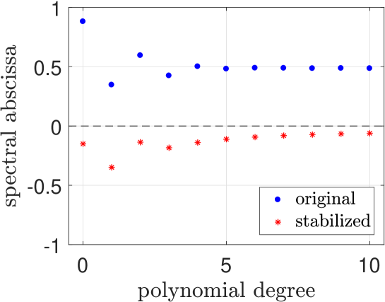
Figure 1: Spectral abscissae in linear dynamical systems, including matrix (23), from stochastic Galerkin method for different polynomial degrees, using a uniform distribution in $[-1,1]$.

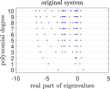
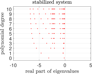
Figure 2: Eigenvalues of the original system, including matrix (23), (left) and the stabilized system (right) for different degrees of the polynomial expansion with uniform distribution in $[-1,1]$.

We repeat the numerical computations employing a uniform distribution in the smaller interval $p\in[-\frac{2}{5},\frac{2}{5}]$. Figure 3 illustrates the spectral abscissae of the Galerkin-projected matrices for different polynomial degrees. Just two out of ten original systems become unstable now. Although the other spectral abscissae of the original system are already negative, the transformed systems exhibit a more negative spectral abscissa. In [14], a similar stabilization technique was applied in the context of model order reduction, where this effect becomes more pronounced in an example.

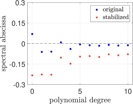
Figure 3: Spectral abscissae in linear dynamical systems, including matrix (23), from stochastic Galerkin method for different polynomial degrees, using a uniform distribution in $[-\frac{2}{5},\frac{2}{5}]$.

Alternatively, we choose a beta distribution in the stochastic modeling. The probability density function reads as

$$\rho(p)=c\,(1-p)^{\alpha}(1+p)^{\beta}\qquad\mbox{for}\;\;p\in[-1,1]$$

with a constant $c>0$ for standardization. We select $\alpha=3$, $\beta=2$. Jacobi polynomials yield an orthogonal basis. Again the stochastic Galerkin method results in unstable systems for all polynomial degrees. The Galerkin projection of the matrices of the original system and the stabilized system are computed by Gauss-Jacobi quadrature with 20 nodes. The spectral abscissae of the Galerkin-projected matrices for the polynomial degrees $d=0,1,\ldots,10$ are depicted in Figure 4. The transformation yields again a stabilization of the critical systems.

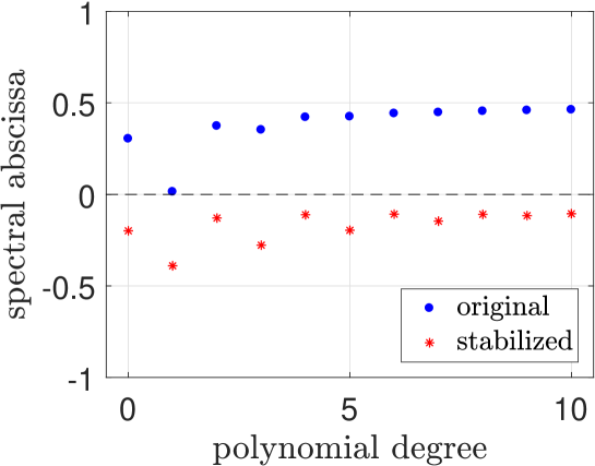
Figure 4: Spectral abscissae in linear dynamical systems, including matrix (23), after the Galerkin projection for different polynomial degrees, using a beta distribution in $[-1,1]$.

5.2 Nonlinear dynamical system

We now consider a two-dimensional dynamical system (13) with the quadratic right-hand side

$$\mbox{}f(x,p)=\footnotesize\begin{pmatrix}x_{1}^{2}+(-35p-2\sin(p)-13p^{2}-97)x_{1}-2x_{2}^{2}+(4\cos(p)-77p-33p^{2}+23)x_{2}\\ +\sin^{2}(p)-2\cos^{2}(p)+\cos(p)(33p^{2}+77p-23)+\sin(p)(13p^{2}+35p+97)\\[6.88889pt] 4x_{1}^{2}+(85p-8\sin(p)+51p^{2}-54)x_{1}-x_{2}^{2}+(2\cos(p)-\frac{1}{10}p+67p^{2}-24)x_{2}\\ +4\sin^{2}(p)-\cos^{2}(p)+\cos(p)(-67p^{2}+\frac{1}{10}p+24)-\sin(p)(51p^{2}+85p-54)\\ \end{pmatrix}$$ (24)

and a real parameter $p$. This system is chosen such that

$$x^{*}(p)=\begin{pmatrix}\sin(p)\\ \cos(p)\\ \end{pmatrix}$$ (25)

is a stationary solution for all $p\in\mathbbm{R}$. Numerical computations confirm that these equilibria are asymptotically stable for all $p\in[-1,1]$. Since the stationary solution (25) includes trigonometric functions, an exact representation in terms of polynomials in the variable $p$ is not feasible.

Again, we assume the parameter to be a uniformly distributed random variable with the range $[-1,1]$. Consequently, the gPC expansion uses the Legendre polynomials. The stochastic Galerkin method yields the nonlinear dynamical system (15). In the right-hand side (16), we evaluate the probabilistic integrals (expected values) approximately by a Gauss-Legendre quadrature using 20 nodes.

Numerical computations show that the Galerkin-projected system (15) exhibits stationary solutions for all degrees $d=1,2,\ldots,10$. Therein, the respective nonlinear systems $F(\hat{v}^{*})=0$ are solved successfully by Newton iterations. The corresponding stationary solutions yield the functions (17), which represent approximations of the equilibrium in the original dynamical system. Figure 5 illustrates the functions (17) for the polynomial degrees $d=1,3,5$. The approximations converge rapidly to sine and cosine, respectively, because these trigonometric terms are analytic functions in the variable $p$. However, the stationary solutions of the Galerkin-projected systems (15) for all polynomial degrees $d$ are unstable, which can be seen by the spectral abscissae of the Jacobian matrices $\left.\frac{\partial F}{\partial\hat{v}}\right|_{\hat{v}=\hat{v}^{*}}$ in Figure 6 (left).

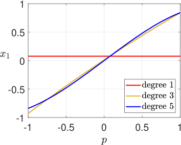
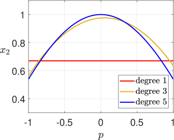
Figure 5: Approximations associated with stationary solutions of the Galerkin-projected system, using the right-hand side function (24), for different polynomial degrees in quadratic problem.

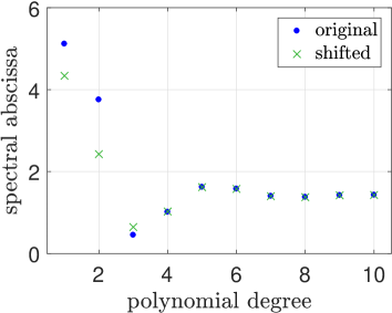
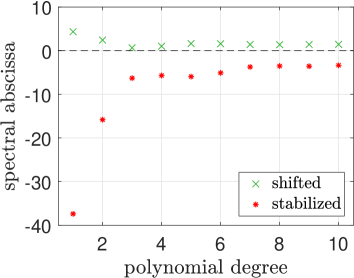
Figure 6: Spectral abscissae for the Jacobian matrices associated with the stationary solutions of the Galerkin projections for the original system, the shifted system and the stabilized system with right-hand side function (24) in the quadratic problem.

To stabilize the computation, we change to the shifted nonlinear dynamical system (18) and its Galerkin-projected system (20). The stationary solutions $\tilde{v}^{*}=0$ are still unstable for all polynomial degrees, which is illustrated by the spectral abscissae of the associated Jacobian matrices in Figure 6 (left). The values for the original Galerkin system and the novel Galerkin system become closer for higher polynomial degrees in agreement to the convergence results in [12].

Now we apply the stabilization technique from Section 4.2. In the Lyapunov equations (11), the matrix $Q=I$, the identity matrix in $\mathbbm{R}^{2\times 2}$, is selected. The Cholesky algorithm yields a decomposition of the solutions. This procedure has to be done for each node of the Gauss-Legendre quadrature. The stochastic Galerkin method projects the transformed system (22) to a larger system (20). Figure 6 (right) shows the spectral abscissae of the Jacobian matrices for the stationary solution zero for different polynomial degrees $d=1,2,\ldots,10$. It follows that the equilibria are asymptotically stable now.

Finally, we illustrate solutions of initial value problems computed using the stochastic Galerkin method for original, shifted and stabilized right-hand side function. We choose the polynomial degree equal to three, which results in eight coefficient functions. The trapezoidal rule yields the numerical solutions. Firstly, the original Galerkin-projected system (15) is solved, whose initial values are selected close to its stationary solution. Figure 7 (top) illustrates the numerical solution. The trajectories are nearly constant at the beginning, say $t\in[0,1]$. Later the solution changes from the unstable equilibrium to some stable equilibrium. Secondly, we solve the Galerkin-projected system (15) with the shifted right-hand side function (18) using initial values $\tilde{v}(0)=(10^{-3},0,\ldots,0)^{\top}$ close to the equilibrium $\tilde{v}^{*}=0$. The same behavior appears like before, as depicted in Figure 7 (center). Thirdly, the Galerkin projection of the stabilized system (22) is solved, where the initial values are set to $\tilde{v}(0)=(1,0,\ldots,0)^{\top}$. Figure 7 (bottom) shows the numerical solution. Now the trajectories tend to the stable stationary solution $\tilde{v}^{*}=0$.

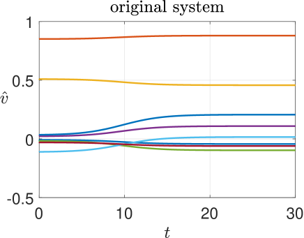
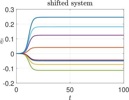
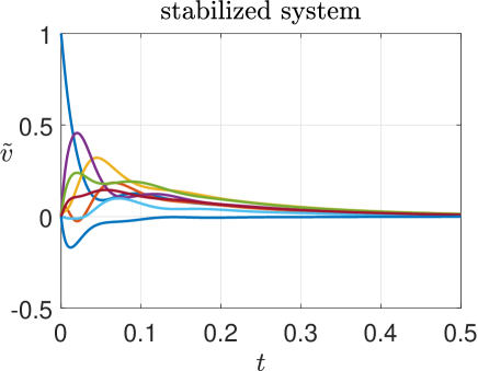
Figure 7: Solutions of initial value problems for the Galerkin projections of original system, shifted system and stabilized system in quadratic test example.

6 Conclusions

A basis transformation was constructed for linear dynamical systems including random variables. We proved that the stability properties are preserved in a Galerkin projection of the transformed system. The transformation matrix follows from a symmetric decomposition of a solution of a Lyapunov equation. We showed that the Cholesky factorization retains the smoothness of involved functions, while the computational effort is low in comparison to eigenvalue/eigenvector decompositions. Moreover, the transformation can be applied to guarantee the stability properties for stationary solutions in nonlinear dynamical systems. We performed numerical computations for test examples. The results demonstrate that the combination of the stochastic Galerkin method and the basis transformation yields an efficient numerical technique to preserve stability of the original system under the Galerkin projection.

References

- [1] F. Augustin, A. Gilg, M. Paffrath, P. Rentrop, U. Wever, Polynomial chaos for the approximation of uncertainties: chances and limits, Euro. Jnl. of Applied Mathematics 19 (2008), pp. 149–190.
- [2] F. Augustin, P. Rentrop, Stochastic Galerkin techniques for random ordinary differential equations, Numer. Math. 122 (2012), pp. 399–419.
- [3] R.H. Bartels, G.W. Stewart, Solution of the matrix equation , Comm. ACM 15 (1972), pp. 820–826.
- [4] O.G. Ernst, A. Mugler, H.J. Starkloff, E. Ullmann, On the convergence of generalized polynomial chaos expansions, ESAIM: Mathematical Modelling and Numerical Analysis 46 (2012), pp. 317–339.
- [5] Z. Gajić, M.T.J. Qureshi, Lyapunov Matrix Equation in System Stability and Control, Dover Publications, Inc., 1995.
- [6] G.H. Golub, C.F. van Loan, Matrix Computations, 4th ed., Johns Hopkins University Press, 2013.
- [7] S.J. Hammarling, Numerical solution of stable non-negative definite Lyapunov equation, IMA J. Numer. Anal. 2 (1982), pp. 303–323.
- [8] E. Hairer, S.P. Nørsett, G. Wanner, Solving Ordinary Differential Equations. Vol. 1: Nonstiff Problems, 2nd ed., Springer, 1993.
- [9] T. Penzl, Numerical solution of generalized Lyapunov equations, Adv. Comput. Math. 8 (1998), pp. 33–48.
- [10] S. Prajna, POD model reduction with stability guarantee, Proceedings of 42nd IEEE Conference on Decision and Control, Maui, Hawaii, USA, December 2003, pp. 5254–5258.
- [11] R. Pulch, Polynomial chaos for linear differential algebraic equations with random parameters, Int. J. Uncertain. Quantif. 1 (2011), pp. 223–240.
- [12] R. Pulch, Stochastic Galerkin methods for analyzing equilibria of random dynamical systems, SIAM/ASA J. Uncertainty Quantification 1 (2013), pp. 408–430.
- [13] R. Pulch, Stochastic collocation and stochastic Galerkin methods for linear differential algebraic equations, J. Comput. Appl. Math. 262 (2014), pp. 281–291.
- [14] R. Pulch, Stability preservation in Galerkin-type projection-based model order reduction, Numer. Algebra Contr. Optim. 9 (2019), pp. 23–44.
- [15] R. Pulch, E.J.W. ter Maten, F. Augustin, Sensitivity analysis and model order reduction for random linear dynamical systems, Math. Comput. Simulat. 111 (2015), pp. 80–95.
- [16] M. Schatzman, Numerical Analysis: A Mathematical Introduction, Clarendon Press, Oxford, 2002.
- [17] R. Seydel, Practical Bifurcation and Stability Analysis, 3rd ed., Springer, 2010.
- [18] N.T. Son, T. Stykel, Solving parameter-dependent Lyapunov equations using the reduced basis method with application to parametric model order reduction, SIAM J. Matrix Anal. Appl. 38 (2017), pp. 478–504.
- [19] B. Sonday, R. Berry, B. Debusschere, H. Najm, Eigenvalues of the Jacobian of a Galerkin-projected uncertain ODE system, SIAM J. Sci. Comput. 33 (2011), pp. 1212–1233.
- [20] J. Stoer, R. Bulirsch, Introduction to Numerical Analysis, 3rd ed., Springer, New York, 2002.
- [21] T.J. Sullivan, Introduction to Uncertainty Quantification, Springer, 2015.
- [22] D. Xiu, Numerical Methods for Stochastic Computations: a Spectral Method Approach, Princeton University Press, 2010.