Associative Domain Adaptation

Abstract

We propose associative domain adaptation, a novel technique for end-to-end domain adaptation with neural networks, the task of inferring class labels for an unlabeled target domain based on the statistical properties of a labeled source domain. Our training scheme follows the paradigm that in order to effectively derive class labels for the target domain, a network should produce statistically domain invariant embeddings, while minimizing the classification error on the labeled source domain. We accomplish this by reinforcing associations between source and target data directly in embedding space. Our method can easily be added to any existing classification network with no structural and almost no computational overhead. We demonstrate the effectiveness of our approach on various benchmarks and achieve state-of-the-art results across the board with a generic convolutional neural network architecture not specifically tuned to the respective tasks. Finally, we show that the proposed association loss produces embeddings that are more effective for domain adaptation compared to methods employing maximum mean discrepancy as a similarity measure in embedding space.

1 Introduction

Since the publication of LeNet [14] and AlexNet [13], a methodological shift has been observable in the field of computer vision. Deep convolutional neural networks have proved to solve a growing number of problems [28, 7, 29, 27, 6, 17]. On the downside, due to a large amount of model parameters, an equally rapidly growing amount of labeled data is needed for training, such as ImageNet [21], comprising millions of labeled training examples. This data may be costly to obtain or even nonexistent.

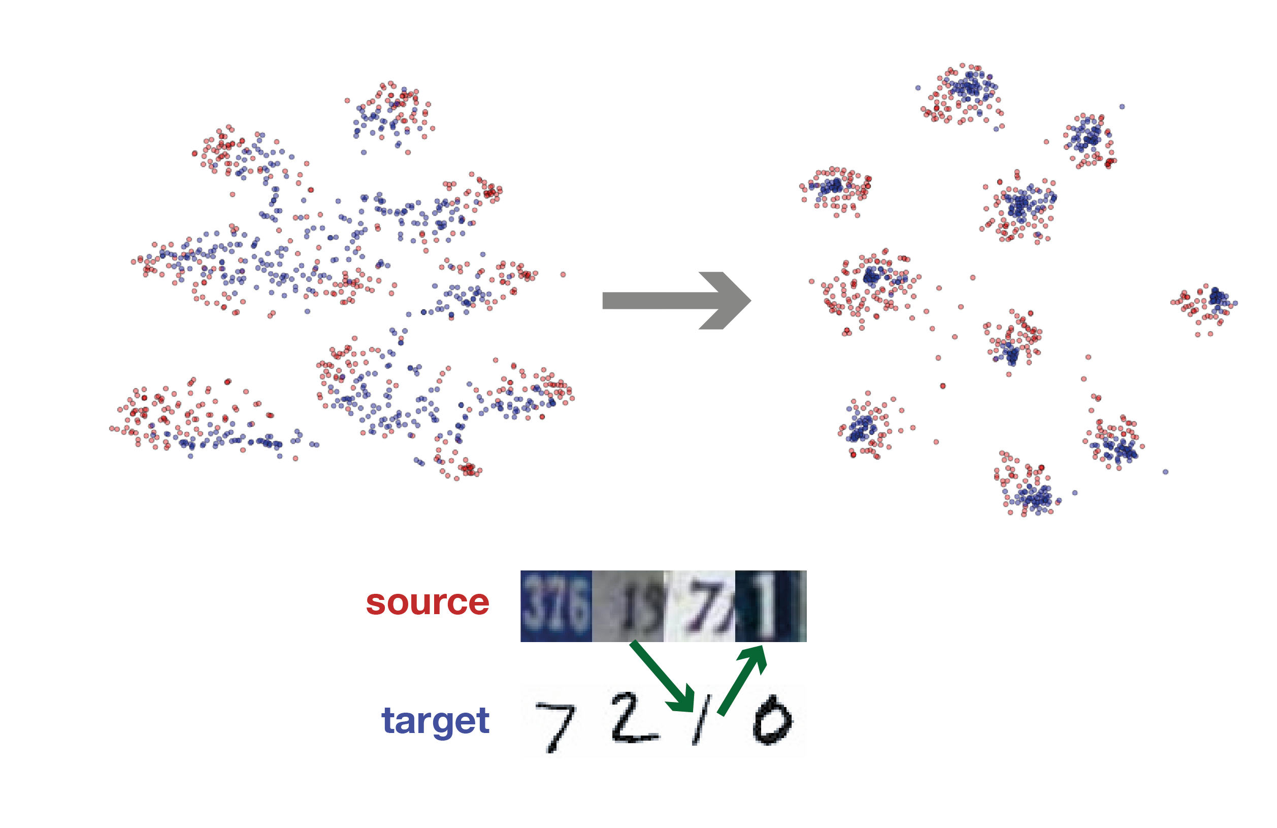
In this paper, we focus on an approach to train neural networks with a minimum of labeled data: domain adaptation. We refer to domain adaptation as the task to train a model on labeled data from a source domain while minimizing test error on a target domain, for which no labels are available at training time.

Figure 1: Associative domain adaptation. In order to maximize classification accuracy on an unlabeled target domain, the discrepancy between neural network embeddings of source and target samples (red and blue, respectively) is reduced by an associative loss ($\color[rgb]{0,0.4,0}\rightarrow$), while minimizing a classification error on the labeled source domain.

1.1 Domain adaptation

In more formal terms, we consider a source domain $\mathcal{D}_{s}=\{\bm{x}_{i}^{s},y_{i}^{s}\}_{i=1,\dots,n_{s}}$ and a target domain $\mathcal{D}_{t}\leavevmode\nobreak\ =\leavevmode\nobreak\ \{\bm{x}_{i}^{t},y_{i}^{t}\}_{i=1,\dots,n_{t}}$. Here, $\bm{x}_{i}^{s}\in\mathbb{R}^{N_{s}},\bm{x}_{i}^{t}\in\mathbb{R}^{N_{t}}$ are the data vectors and $y_{i}^{s}\in\mathcal{C},y_{i}^{t}\in\mathcal{C}$ the respective labels, where the target labels $\{y_{i}^{t}\}_{i=1,\dots,n_{t}}$ are not available for training. Note that for domain adaption it is assumed that source and target domains are associated with the same label space, while $\mathcal{D}_{s}$ and $\mathcal{D}_{t}$ are drawn from distributions $\mathbb{P}_{s}$ and $\mathbb{P}_{t}$, which are assumed to be different, i.e. the source and target distribution have different joint distributions of data $\bm{X}$ and labels $\bm{Y}$, $\mathbb{P}_{s}(\bm{X},\bm{Y})\neq\mathbb{P}_{t}(\bm{X},\bm{Y})$.

The value of domain adaptation has even more increased with generative tools producing synthetic datasets. The idea is compelling: rather than labeling vast amounts of real-world data, one renders a similar but synthetic dataset that is automatically labeled. With an effective method for domain adaptation it becomes possible to train models without the need for one single labeled target example at training time.

In order to combine labeled and unlabeled data for a predictive task, a variety of notions has emerged. To be clear, we explicitly distinguish domain adaptation from related approaches. For semi-supervised learning, labeled source data is leveraged by unlabeled target data drawn from the same distribution, i.e. $\mathbb{P}_{s}=\mathbb{P}_{t}$. In transfer learning, not only source and target domain are drawn from different distributions, also their label spaces are generally different. An example of supervised transfer learning is training a neural network on a source domain and subsequently fine-tuning the model on a labeled target domain for a different task [33, 5].

The problem of domain adaptation was theoretically studied in [2], relating source and target error with a statistical similarity measure of the respective domains. Their results suggest that a good domain adaptation method should be based on features that are as similar as possible for source and target domain (assimilation), while reducing the prediction error in the source domain as much as possible (discrimination). These effects are opposing each other since source and target domains are drawn from different distributions. This can be formulated as a cost function that consists of two terms:

$$\mathcal{L}=\mathcal{L_{\mathrm{classification}}}+\mathcal{L_{\mathrm{sim}}}\;,$$ (1)

Here, the classification loss, $\mathcal{L_{\mathrm{classification}}}$ encourages discrimination between different classes, maximizing the margin between clusters of embeddings that belong to the same class. We define the second term as a generic similarity loss $\mathcal{L_{\mathrm{sim}}}$, which enforces statistically similar latent representations.

Intuitively, for similar latent representations of the source and target domain, the target class labels can be more accurately inferred from the labeled source samples.

In the following, we show how previous methods approached this optimization and then propose a new loss for $\mathcal{L_{\mathrm{sim}}}$.

1.2 Related work

Several works have approached the problem of domain adaptation. Here, we mainly focus on methods that are based on deep learning, as these have proved to be powerful learning systems and are closest to our scheme.

The CORAL method [24] explicitly forces the covariance of the target data onto the source data (assimilation). The authors then apply supervised training to this transformed source domain with original labels (discrimination). This idea is extended to second order statistics of features in deep neural networks in [25].

Building on the idea of adversarial training [10], the authors of [9] propose an architecture in which a class label and a domain label predictor are built on top of a general feature extractor. While the class label predictor is supposed to correctly classify the labeled training examples (discrimination), the domain label predictor for all training samples is used in a way to make the feature distributions similar (assimilation). The authors of [3] use an adversarial approach to train for similarity in data space instead of feature space. Their training scheme is closer to standard generative adversarial networks [10], however, it does not only condition on noise, but also on an image from the source domain.

Within the paradigm of training for domain invariant features, one popular metric is the maximum mean discrepancy (MMD) [11]. This measure is the distance between the mean embeddings of two probability distributions in a reproducing kernel Hilbert space $\mathcal{H}_{k}$ with a characteristic kernel $k$. More precisely, the mean embedding of a distribution $\mathbb{P}$ in $\mathcal{H}_{k}$ is the unique element $\mu_{k}(\mathbb{P})\in\mathcal{H}_{k}$ such that $\mathbb{E}_{x\sim\mathbb{P}}[f(x)]=\left\langle f(x),\mu_{k}(\mathbb{P})\right\rangle_{\mathcal{H}_{k}},\forall f\in\mathcal{H}_{k}$. The MMD distance between source and target domain then reads $d_{\mathrm{MMD}}(\mathbb{P}_{s},\mathbb{P}_{t})=||\mu_{k}(\mathbb{P}_{s})-\mu_{k}(\mathbb{P}_{t})||_{\mathcal{H}_{k}}$. In practice, this distance is computed via the kernel trick [31], which leads to an algorithm with quadratic runtime in the number of samples. Linear time estimators have previously been proposed [15].

Most works, which explicitly minimize latent feature discrepancy, use MMD in some variant. That is, they use MMD as $\mathcal{L_{\mathrm{sim}}}$ in order to achieve assimilation as defined above. The authors of [15] propose the Deep Adaptation Network architecture. Exploiting that learned features transition from general to specific within the network, they train the first layers of a CNN commonly for source and target domain, then train individual task-specific layers while minimizing the multiple kernel maximum mean discrepancies between these layers.

The technique of task-specific but coupled layers is further explored in [20] and [4]. The authors of [20] propose to individually train source and target domains while the network parameters of each layer are regularized to be linear transformations of each other. In order to train for domain invariant features, they minimize the MMD of the embedding layer. On the other hand, the authors of [4] maintain a shared representation of both domains and private representations of each individual domain in their Domain Separation architecture.

As becomes evident in these works, the MMD minimizes domain discrepancy in some abstract space and requires a choice of kernels with appropriate hyperparameters, such as the standard deviation of the Gaussian kernel. In this work, we propose a different loss for $\mathcal{L_{\mathrm{sim}}}$ which is more intuitive in embedding space, less computationally complex and better suitable to obtain effective embeddings.

1.3 Contribution

We propose the association loss $\mathcal{L_{\mathrm{assoc}}}$ as an alternative discrepancy measure ($\mathcal{L_{\mathrm{sim}}}$) within the domain adaptation paradigm described in Section 1.1. The reasoning behind our approach is the following: Ultimately, we want to minimize the classification error on the target domain $\mathcal{D}_{t}$. This is not directly possible since no labels are available at training time. Therefore, we minimize the classification error on the source domain $\mathcal{D}_{s}$ as a proxy while enforcing representations of $\mathcal{D}_{t}$ to have similar statistics to those of $\mathcal{D}_{s}$. This is accomplished by enforcing associations [12] between feature representations of $\mathcal{D}_{t}$ with those of $\mathcal{D}_{s}$ that are in the same class. Therefore, in contrast to MMD as $\mathcal{L_{\mathrm{sim}}}$, this approach also leverages knowledge about labels of the source domain and hence avoids unwanted assimilation across class clusters. The implementation is simple yet powerful as we show in Section 2. It works with any existing architecture and, unlike most deep learning approaches for domain adaptation, does not introduce a structural and almost no computational overhead. In fact, we used the same generic and simple architecture for all our experiments, each of which achieved state-of-the-art results.

In summary, our contributions are:

• A straightforward training schedule for domain adaptation with neural networks.

• An integration of our approach into the prevailing domain adaptation formalism and a detailed comparison with the most commonly used explicit $\mathcal{L_{\mathrm{sim}}}$: the maximum mean discrepancy (MMD).

• A simple implementation that works with arbitrary architectures.

• Extensive experiments on various benchmarks for domain adaptation that outperform related deep learning methods.

• A detailed analysis demonstrating that associative domain adaptation results in effective embeddings in terms of classifying target domain samples.

2 Associative domain adaptation

We start from the approach of learning by association [12] which is geared towards semi-supervised training. Labeled and unlabeled data are related by associating their embeddings, i.e. features of a neural network’s last layer before the softmax layer. Our work generalizes this approach for domain adaptation. For the new task, we identify labeled data with the source domain and unlabeled data with the target domain. Specifically, for $\bm{x}_{i}^{s}\in\mathcal{D}_{s},\bm{x}_{i}^{t}\in\mathcal{D}_{t}$ and the embedding map $\phi:\mathbb{R}^{N_{0}}\rightarrow\mathbb{R}^{N_{L-1}}$ of an $L$-layer neural network, denote by $A_{i}\mathrel{\vbox{\hbox{\scriptsize.}\hbox{\scriptsize.}}}=\phi(\bm{x}_{i}^{s}),B_{j}\mathrel{\vbox{\hbox{\scriptsize.}\hbox{\scriptsize.}}}=\phi(\bm{x}_{j}^{t})$ the respective embeddings of source and target domain. Then, similarity is measured by the embedding vectors’ dot product as $M_{ij}=\left\langle A_{i},B_{j}\right\rangle$.

If one considers transitions between the parts $(\{A_{i}\},\{B_{j}\})$ of a bipartite graph, the intuition is that transitions are more probable if embeddings are more similar. This is formalized by the transition probability from embedding $A_{i}$ to embedding $B_{j}$:

$$P_{ij}^{ab}=\mathbb{P}(B_{j}|A_{i})\mathrel{\vbox{\hbox{\scriptsize.}\hbox{\scriptsize.}}}=\frac{\exp(M_{ij})}{\sum_{j^{\prime}}\exp(M_{ij^{\prime}})}\;.$$ (2)

The basis of associative similarity is the two-step round-trip probability of an imaginary random walker starting from an embedding $A_{i}$ of the labeled source domain and returning to another embedding $A_{j}$ via the (unlabeled) target domain embeddings $B$,

$$P_{ij}^{aba}\mathrel{\vbox{\hbox{\scriptsize.}\hbox{\scriptsize.}}}=\left(P^{ab}P^{ba}\right)_{ij}\;.$$ (3)

The authors of [12] observed that higher order round trips do not improve performance. The two-step probabilities are forced to be similar to the uniform distribution over the class labels via a cross-entropy loss term called the walker loss,

$$\mathcal{L_{\mathrm{walker}}}\mathrel{\vbox{\hbox{\scriptsize.}\hbox{\scriptsize.}}}=H\left(T,P^{aba}\right)\;,$$ (4)

where

$$T_{ij}\mathrel{\vbox{\hbox{\scriptsize.}\hbox{\scriptsize.}}}=\begin{cases}1/|A_{i}|&\mathrm{class}(A_{i})=\mathrm{class}(A_{j})\\ 0&\mathrm{else}\end{cases}$$ (5)

This means that all association cycles within the same class are forced to have equal probability. The walker loss by itself could be minimized by only visiting target samples that are easily associated, skipping difficult examples. This would lead to poor generalization to the target domain. Therefore, a regularizer is necessary such that each target sample is visited with equal probability. This is the function of the visit loss. It is defined by the cross entropy between the uniform distribution over target samples and the probability of visiting some target sample starting in any source sample,

$$\mathcal{L_{\mathrm{visit}}}\mathrel{\vbox{\hbox{\scriptsize.}\hbox{\scriptsize.}}}=H(V,P^{\mathrm{visit}})\;,$$ (6)

where

$$P_{j}^{\mathrm{visit}}\mathrel{\vbox{\hbox{\scriptsize.}\hbox{\scriptsize.}}}=\sum_{\bm{x}_{i}\in\mathcal{D}_{s}}P_{ij}^{ab},\quad V_{j}\mathrel{\vbox{\hbox{\scriptsize.}\hbox{\scriptsize.}}}=\frac{1}{|B|}\,.$$ (7)

Note that this formulation assumes that the class distribution is the same for source and target domain. If this is not the case, using a low weight for $\mathcal{L_{\mathrm{visit}}}$ may yield better results.

Together, these terms form a loss that enforces associations between similar embeddings of both domains,

$$\mathcal{L_{\mathrm{assoc}}}=\beta_{1}\mathcal{L_{\mathrm{walker}}}+\beta_{2}\mathcal{L_{\mathrm{visit}}}\;,$$ (8)

where $\beta_{i}$ is a weight factor. At the same time, the network is trained to minimize the prediction error on the labeled source data via a softmax cross-entropy loss term, $\mathcal{L_{\mathrm{classification}}}$.

The overall neural network loss for our training scheme is given by

$$\mathcal{L}=\mathcal{L_{\mathrm{classification}}}+\alpha\mathcal{L_{\mathrm{assoc}}}\;.$$ (9)

We want to emphasize once more the essential motivation for our approach: The association loss enforces similar embeddings (assimilation) for the source and target samples, while the classification loss minimizes the prediction error of the source data (discrimination). Without $\mathcal{L_{\mathrm{assoc}}}$, we have the case of a neural network that is trained conventionally [13] on the source domain only. As we show in this work, the (scheduled) addition of $\mathcal{L_{\mathrm{assoc}}}$ during training allows to incorporate unlabeled data from a different domain improving the effectiveness of embeddings for classification. Adding $\mathcal{L_{\mathrm{assoc}}}$ enables an arbitrary neural network to be trained for domain adaptation. The neural network learning algorithm is then able to model the shift in distribution between source and target domain. More formally, if $\mathcal{L_{\mathrm{assoc}}}$ is minimized, associated embeddings from both source and target domain become more similar in terms of their dot product.

In contrast to MMD, $\mathcal{L_{\mathrm{assoc}}}$ incorporates knowledge about source domain classes and hence prevents the case that source and target domain embeddings are statistically similar, but not class discriminative. We demonstrate this experimentally in Section 3.4.

We emphasize that not every semi-supervised training method can be adapted for domain adaptation in this manner. It is necessary that the method explicitly models the shift between the source and target distributions, in order to reduce the discrepancy between both domains, which is accomplished by $\mathcal{L_{\mathrm{assoc}}}$.

In this respect, associative domain adaptation parallels the approaches mentioned in Section 1.2. As we demonstrate experimentally in the next section, $\mathcal{L_{\mathrm{assoc}}}$ is employed as a compact, intuitive and effective training signal for assimilation yielding superior performance on all tested benchmarks.

3 Experiments

MNIST $\big{\Downarrow}$ MNIST-M (10 classes)
Synth $\big{\Downarrow}$ SVHN (10 classes)
SVHN $\big{\Downarrow}$ MNIST (10 classes)
Synth Signs $\big{\Downarrow}$ GTSRB (43 classes)

Table 1: Dataset samples for our domain adaptation tasks. For three randomly chosen classes, the first row depicts a source sample, the second row a target sample. The datasets vary in difficulty due to differences in color space, variance of transformation or number of classes.

Method	Domains (source $\rightarrow$ target)
	MNIST $\rightarrow$ MNIST-M	Syn. Digits $\rightarrow$ SVHN	SVHN $\rightarrow$ MNIST	Syn. Signs $\rightarrow$ GTSRB
Transf. Repr. [22]	13.30	-	21.20	-
SA [8]	43.10	13.56	40.68	18.35
CORAL [24]	42.30	14.80	36.90	13.10
ADDA [30]	-	-	24.00	-
DANN [9]	23.33 (55.87 %)	8.91 (79.67 %)	26.15 (42.57 %)	11.35 (46.39 %)
DSN w/ DANN [3]	16.80 (63.18 %)	8.80 (78.95 %)	17.30 (58.31 %)	6.90 (54.42 %)
DSN w/ MMD [3]	19.50 (56.77 %)	11.50 (31.58 %)	27.80 (32.26 %)	7.40 (51.02 %)
MMD [15]	23.10	12.00	28.90	8.90
$\mathrm{DA}_{\mathrm{MMD}}$	22.90	19.14	28.48	10.69
Ours ($\mathrm{DA}_{\mathrm{assoc}}$ fixed params†)	10.47 $\pm$ 0.28	8.70 $\pm$ 0.2	4.32 $\pm$ 1.54	17.20 $\pm$ 1.32
Ours ($\mathrm{DA}_{\mathrm{assoc}}$)	10.53 (85.94 %)	8.14 (87.78 %)	2.40 (93.71 %)	2.34 (81.23)
Source only	35.96	15.68	30.71	4.59
Target only	6.37	7.09	0.50	1.82

Table 2: Domain adaptation. Errors (%) on the target test sets (lower is better). Source only and target only refer to training only on the respective dataset (supervisedly [12], without domain adaptation) and evaluating on the target dataset. In the $\mathrm{DA}_{\mathrm{MMD}}$ setting, we replaced $\mathcal{L_{\mathrm{assoc}}}$ with MMD. The metric coverage is reported in parentheses, where available (cf. Section 3.3). We used the same network architecture for all our experiments and achieve state of the art results on all benchmarks. The row “$\mathrm{DA}_{\mathrm{assoc}}$ fixed params^†” reports results from 10 runs ($\pm$ standard deviation) with an arbitrary choice of fixed hyper parameters ($\beta_{2}$ = 0.5, delay = 500 steps and batch size = 100) for all four domain pairs. The row below shows our results after individual hyper parameter optimization. No labels of the target domain were used at training time.

3.1 Domain adaptation benchmarks

In order to evaluate and compare our method, we chose common domain adaptation tasks, for which previous results are reported. Examples for the respective datasets are shown in Table 1.

MNIST $\rightarrow$ MNIST-M

We used the MNIST [14] dataset as labeled source and generated the unlabeled MNIST-M target as described in [9]. Background patches from the color photo BSDS500 dataset [1] were randomly extracted. Then the absolute value of the difference of each color channel with the MNIST image was taken. This yields a color image, which can be easily identified by a human, but is significantly more difficult for a machine compared to MNIST due to two additional color channels and more nuanced noise. The single channel of the MNIST images was replicated three times to match those of the MNIST-M images (RGB). The image size is $28\times 28$ pixels. This is the only setting where we used data augmentation: We randomly inverted MNIST images since they are always white on black, unlike MNIST-M.

Synth $\rightarrow$ SVHN

The Street View House Numbers (SVHN) dataset [19] contains house number signs extracted from Google Street View. We used the variant Format 2 where images ($32\times 32$ pixels) are already cropped. Still, multiple digits can appear in one image. As a labeled source domain we use the Synthetic Digits dataset provided by the authors of [9], which expresses a varying number of fonts and properties (background, orientation, position, stroke color, blur) that aim to mimic the distribution in SVHN.

SVHN $\rightarrow$ MNIST

MNIST images were resized with bilinear interpolation to $32\times 32$ pixels and extended to three channels in order to match the shape of SVHN.

Synthetic Signs $\rightarrow$ GTSRB

The Synthetic Signs dataset was provided by the authors of [18] and consists of 100,000 images that were generated by taking common street signs from Wikipedia and applying various artificial transformations. The German Traffic Signs Recognition Benchmark (GTSRB) [23] provides 39,209 (training set) and 12,630 (test set) cropped images of German traffic signs. The images vary in size and were resized with bilinear interpolation to match the Synthetic Signs images’ size of $40\times 40$ pixels. Both datasets contain images from 43 different classes.

3.2 Training setup

3.2.1 Associative domain adaptation

Our formulation of associative domain adaptation is implemented as a custom loss function that can be added to any existing neural network architecture. Results obtained by neural network learning algorithms often highly depend on the complexity of a specifically tuned architecture. Since we wanted to make the effect of our approach as transparent as possible, we chose the following generic convolutional neural network architecture for all our experiments:

$$C(32,3)\rightarrow C(32,3)\rightarrow P(2)$$

$$\rightarrow\; C(64,3)\rightarrow C(64,3)\rightarrow P(2)$$

$$\rightarrow\; C(128,3)\rightarrow C(128,3)\rightarrow P(2)\rightarrow FC(128)$$

Here, $C(n,k)$ stands for a convolutional layer with n kernels of size $k\times k$ and stride 1. $P(k)$ denotes a max-pooling layer with window size $k\times k$ and stride 1. $FC(n)$ is a fully connected layer with $n$ output units. The size of the embeddings is 128. An additional fully connected layer maps these embeddings to logits, which are the input to a softmax cross-entropy loss for classification, $\mathcal{L_{\mathrm{classification}}}$.

The detailed hyperparameters for each experiment can be found in the supplementary material. The most important hyperparameters are the following:

Learning rate

We chose the same initial learning rate ($\tau=1e^{-4}$) for all experiments, which was reduced by a factor of $0.33$ in the last third of the training time. All trainings converged in less than 20k iterations.

Mini-batch sizes

It is important to ensure that a mini-batch represents all classes sufficiently, in order not to introduce a bias. For the labeled mini-batch, we explicitly sample a number of examples per class. For the unlabeled mini-batch we chose the same overall size as for the labeled one, usually around 10-100 times the number of classes.

Loss weights

The only loss weight that we actively chose is the one for $\mathcal{L_{\mathrm{visit}}}$, $\beta_{2}$. As was shown in [12], this loss acts as a regularizer. Since it assumes the same class distribution on both domains, the weight needs to be lowered if the assumption does not hold. We experimentally chose a suitable weight.

Delay of $\mathcal{L_{\mathrm{assoc}}}$

We observed that convergence is faster if we first train the network only with the classification loss, $\mathcal{L_{\mathrm{classification}}}$, and then add the association loss, $\mathcal{L_{\mathrm{assoc}}}$, after a number of iterations. This is implemented by defining $\alpha$ (Equation 8) as a step function. This procedure is intuitive, as the transfer of label information from source to target domain is most effective when the network has already learned some class structure and the embeddings are not random anymore.

Figure 2: t-SNE embeddings with perplexity $35$ of 1,000 test samples for Synthetic Digits (source, red) and SVHN (target, blue). Left: After training on source only. Middle: after training with associative domain adaptation ($\mathrm{DA}_{\mathrm{assoc}}$). Right: after training with MMD loss ($\mathrm{DA}_{\mathrm{MMD}}$). While the target samples are diffuse when embedded with the source only trained network, the class label information is successfully inferred after associative domain adaptation. When the network is trained with an MMD loss, the resulting distributions are similar, but less visibly class discriminative.

	Domains (source $\rightarrow$ target)
	MNIST $\rightarrow$ MNIST-M	Syn. Digits $\rightarrow$ SVHN	SVHN $\rightarrow$ MNIST	Syn. Signs $\rightarrow$ GTSRB
Source only	0.1234 (35.96)	0.1010 (15.68)	0.0739 (30.71)	0.0466 (4.59)
$\mathrm{DA}_{\mathrm{assoc}}$	0.0504 (10.53)	0.0415 (8.14)	0.2112 (2.40)	0.0459 (2.34)
$\mathrm{DA}_{\mathrm{MMD}}$	0.0233 (22.90)	0.0166 (19.29)	0.0404 (34.06)	0.0145 (12.85)

Table 3: Maximum mean discrepancy (MMD) between embeddings of source and target domain, obtained with a network trained supervisedly on source only (SO), for the domain adaptation setting with $\mathcal{L_{\mathrm{assoc}}}$ ($\mathrm{DA}_{\mathrm{assoc}}$) and with an MMD loss ($\mathrm{DA}_{\mathrm{MMD}}$). Numbers in parentheses are test errors on the target domain from Table 2. Associative domain adaptation also reduces the MMD in some cases. Lower MMD values do not correlate with lower test errors. In fact, even though the MMD for training with the associative loss is higher compared with training with the MMD loss, our approach achieves lower test errors.

Hyper parameter tuning

We are aware that hyper parameter tuning can sometimes obscure the actual effect of a proposed method. In particular, we want to discuss the effect of small batch sizes on our algorithm. For the association loss to work properly, all classes must be represented in a mini-batch, which places a restriction on small batch sizes, when the number of classes is large. To further investigate this hyperparameter we ran the same architecture with an arbitrary choice of fixed hyper parameters and smaller batch size ($\beta_{2}$ = 0.5, delay = 500 steps and batch size = 100) for all four domain pairs and report the mean and standard deviation of 10 runs in the row “$\mathrm{DA}_{\mathrm{assoc}}$ fixed params^†”. In all cases except for the traffic signs, these runs outperform previous methods. The traffic sign setup is special because there are 4.3$\times$ more classes and with larger batches more classes are expected to be present in the unlabeled batch. When we removed the batch size constraint, we achieved a test error of 6.55 $\pm$ 0.59, which outperforms state of the art for the traffic signs.

Hardware

All experiments were carried out on an NVIDIA Titan X (Pascal). Each experiment took less than 120 minutes until convergence.

3.2.2 Domain adaptation with MMD

In order to compare our setup and the proposed $\mathcal{L_{\mathrm{assoc}}}$, we additionally ran all experiments described above with MMD instead of $\mathcal{L_{\mathrm{assoc}}}$. We performed the same hyperparameter search for $\alpha$ and report the respectively best test errors. We used the open source implementation including hyperparameters from [26]. This setup is referred to as $\mathrm{DA}_{\mathrm{MMD}}$.

3.3 Evaluation

All reported test errors are evaluated on the target domain. To assess the quality of domain adaptation, we provide results trained on source and target only (SO and TO, respectively) as in [12], for associative domain adaptation ($\mathrm{DA}_{\mathrm{assoc}}$) and for the same architecture with MMD instead of $\mathcal{L_{\mathrm{assoc}}}$. Besides the absolute accuracy, an informative metric is coverage of the gap between TO and SO by DA,

$$\frac{DA-SO}{TO-SO}\;,$$

as it is a measure of how much label information is successfully transferred from the source to the target domain. In order to assess a method’s performance on domain adaptation, one should always consider both coverage and absolute error on the target test set since a high coverage could also stem from poor performance in the SO or TO setting.

Where available, we report the coverage of other methods (with respect to their own performance on SO and TO).

Table 2 shows the results of our experiments. In all four popular domain adaptation settings our method performs best. On average, our approach improves the performance by 87.17 % compared to training on source only (coverage). In order to make our results as comparable as possible, we used a generic architecture that was not handcrafted for the respective tasks (cf. Section 3.2).

3.4 Analysis of the embedding quality

As described in Section 1, a good intuition for the formalism of domain adaptation is the following. On the one hand, the latent features should cluster in embedding space, if they belong to the same class (assimilation). On the other hand, these clusters should separate well in order to facilitate classification (discrimination).

We claim that our proposed $\mathcal{L_{\mathrm{assoc}}}$ is well suited for this task compared with maximum mean discrepancy. We use four points to support this claim:

• t-SNE visualizations show that employing $\mathcal{L_{\mathrm{assoc}}}$ produces embeddings that cluster better compared to MMD.

• $\mathcal{L_{\mathrm{assoc}}}$ simultaneously reduces the maximum mean discrepancy (MMD) in most cases.

• Lower MMD values do not imply lower target test errors in these settings.

• In all cases, the target domain test error of our approach is lower compared to training with an MMD loss.

3.4.1 Qualitative evaluation: t-SNE embeddings

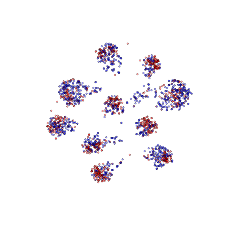
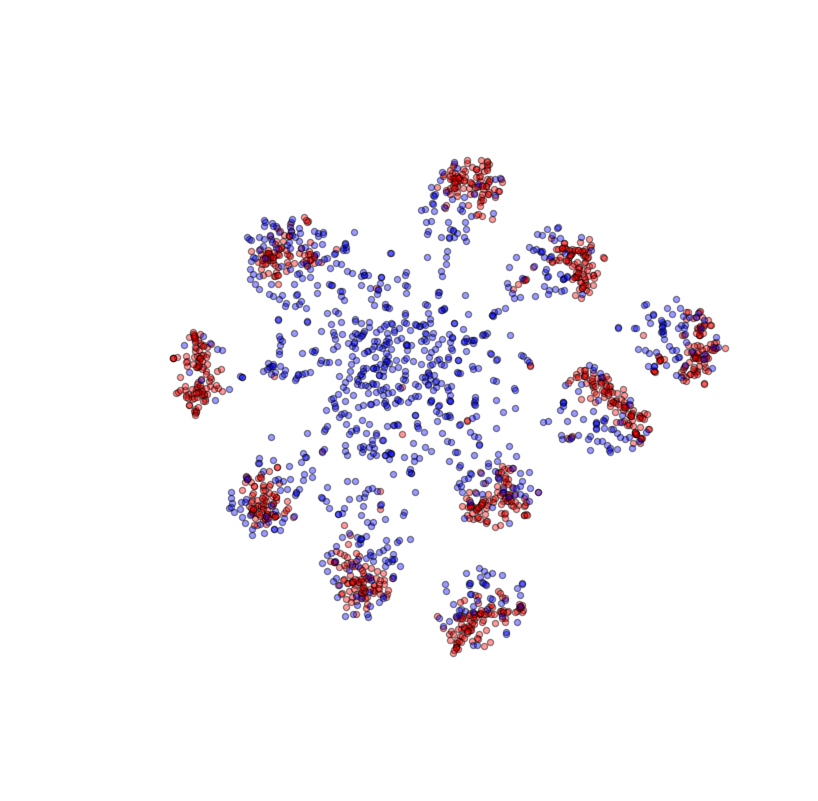
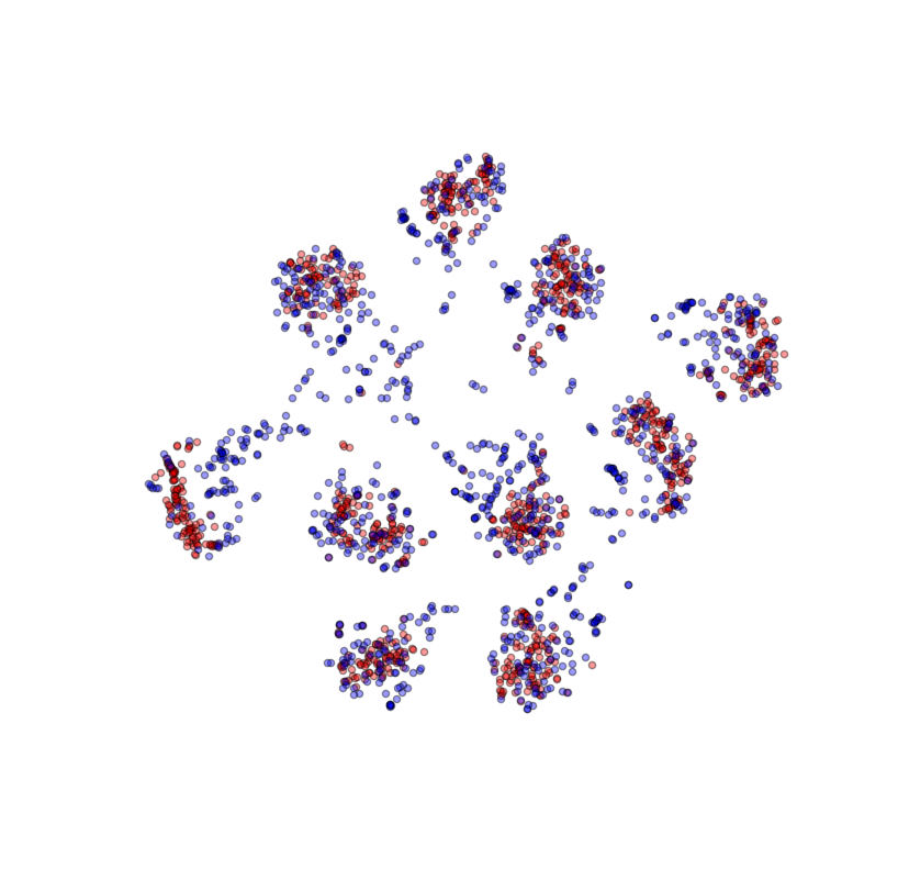
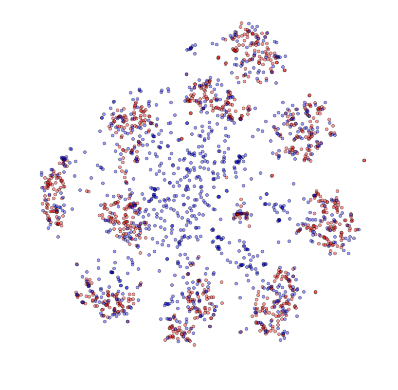
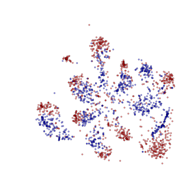
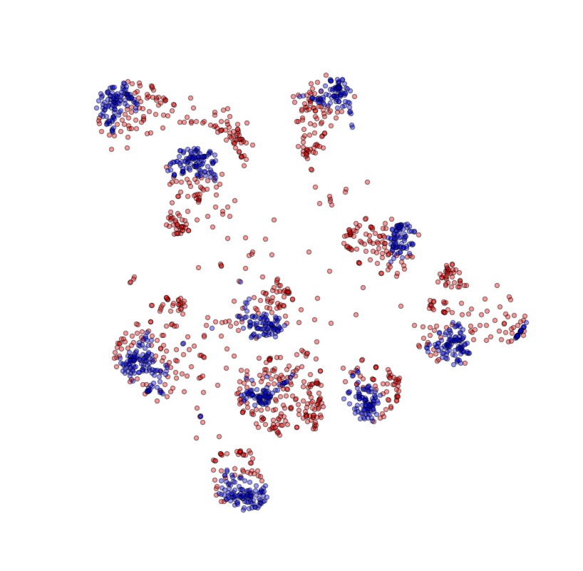
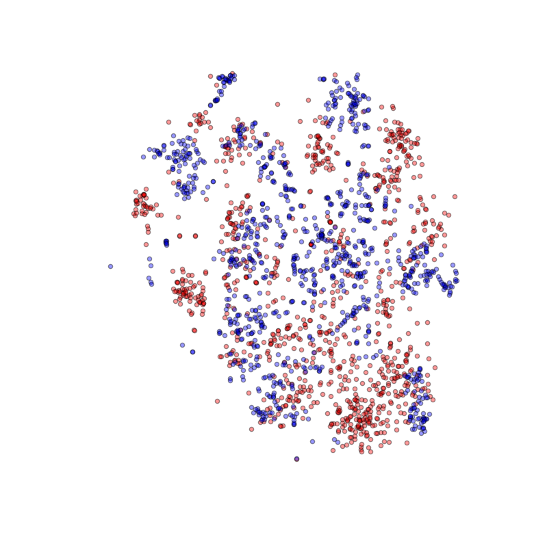
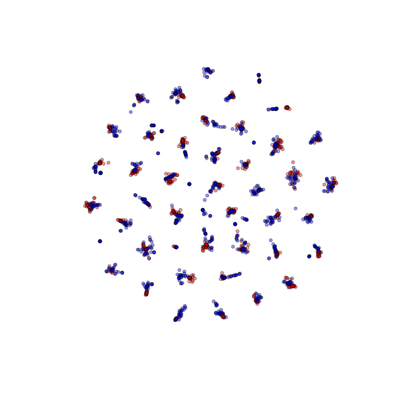
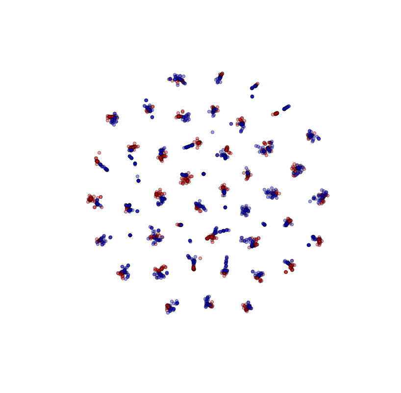
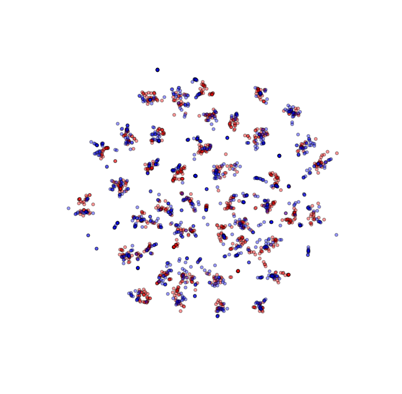
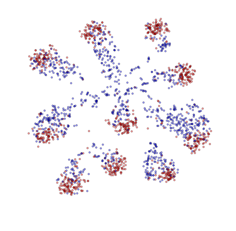
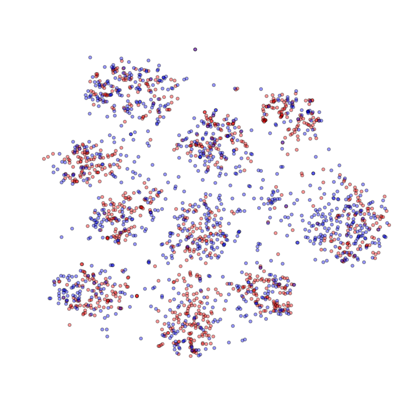
A popular method to visualize high-dimensional data in 2D is t-SNE [16]. We are interested in the distribution of embeddings for source and target domain when we employ our training scheme. Figure 2 shows such visualizations. We always plotted embeddings of the target domain test set. The embeddings are obtained with networks trained semi-supervisedly [12] on the source domain only (SO), with our proposed associative domain adaptation ($\mathrm{DA}_{\mathrm{assoc}}$) and with MMD instead of $\mathcal{L_{\mathrm{assoc}}}$ ($\mathrm{DA}_{\mathrm{MMD}}$, cf. Section 3.2).

In the SO setting, samples from the source domain fall into clusters as expected. Samples from the target domain are more scattered. For $\mathrm{DA}_{\mathrm{assoc}}$, samples from both domains cluster well and become separable. For $\mathrm{DA}_{\mathrm{MMD}}$, the resulting distributions are similar, but not visibly class discriminative.

For completeness, however, we explicitly mention that t-SNE embeddings are obtained via a non-linear, stochastic optimization procedure that depends on the choice of parameters like the perplexity ([16, 32]). We therefore interpret these plots only qualitatively and infer that associative domain adaptation learns consistent embeddings for source and target domain that cluster well with observable margins.

3.4.2 Quantitative evaluation: MMD values

While t-SNE plots provide qualitative insights into the latent feature representation of a learning algorithm, we want to complement this with a quantitative evaluation and compute the discrepancy in embedding space for target and source domains. We estimated the MMD with a Gaussian RBF kernel using the TensorFlow implementation provided by the authors of [26].

The results are shown in Table 3. In parentheses we copied the test accuracies on the respective target domains from Table 2.

We observe that $\mathrm{DA}_{\mathrm{MMD}}$ yields the lowest maximum mean discrepancy, as expected, since this training setup explicitly minimizes this quantity. At the same time, $\mathrm{DA}_{\mathrm{assoc}}$ also reduces this metric in most cases. Interestingly though, for the setup SVHN $\rightarrow$ MNIST, we actually obtain a particularly high MMD. Nevertheless, the test error of the network trained with $\mathrm{DA}_{\mathrm{assoc}}$ is one of the best results. We ascribe this to the fact that MMD enforces domain invariant feature representations regardless of the source labels, whereas $\mathcal{L_{\mathrm{assoc}}}$ takes into account the labels of associated source samples, resulting in better separation of the clusters and higher similarity within the same class. Consequently, $\mathrm{DA}_{\mathrm{assoc}}$ achieves lower test error on the target domain, which is the actual goal of domain adaptation.

4 Conclusion

We have introduced a novel, intuitive domain adaptation scheme for neural networks termed associative domain adaptation that generalizes a recent approach for semi-supervised learning[12] to the domain adaptation setting. The key idea is to optimize a joint loss function combining the classification loss on the source domain with an association loss that imposes consistency of source and target embeddings. The implementation is simple, works with arbitrary architectures in an end-to-end manner and introduces no significant additional computational and structural complexity. We have demonstrated the capabilities of associative domain adaptation on various benchmarks and achieved state-of-the-art results for all our experiments. Finally, we quantitatively and qualitatively examined how well our approach reduces the discrepancy between network embeddings from the source and target domain. We have observed that, compared to explicitly modelling the maximum mean discrepancy as a cost function, the proposed association loss results in embeddings that are more effective for classification in the target domain, the actual goal of domain adaptation.

We provide additional information that is necessary to reproduce our results, as well as plots complementing the evaluation section of the main paper. To this end, we begin by stating implementation details for our neural network learning algorithm. Furthermore, we show additional t-SNE embeddings of source target domain for the different domain adaptation tasks analyzed in the paper.

1 Hyperparameters

We report the hyperparameters that we used for our experiments for the sake of reproducibility as detailed in Table 1.

Hyperparameter	Domains (source $\rightarrow$ target)
	MNIST $\rightarrow$ MNIST-M	Syn. Digits $\rightarrow$ SVHN	SVHN $\rightarrow$ MNIST	Syn. Signs $\rightarrow$ GTSRB
New width/height	32	-	32	-
Source domain batch size	1000	1000	1000	1032
Target domain batch size	1000	1000	1000	1032
Learning rate decay steps	9000	9000	9000	9000
Visit loss weight	0.6	0.2	0.2	0.1
Delay (steps) for $\mathcal{L_{\mathrm{assoc}}}$	500	2000	500	0

Table 1: Hyperparameters for our domain adaptation experiments.

2 t-SNE embeddings

We complement our analysis in Section 3.4.1 of the main document, Qualitative evaluation: t-SNE embeddings. In Figure 1 we show the t-SNE embeddings for all domain adaptation tasks that we have analyzed (cf. Table 3 of the main paper). The qualitative interpretation that we provide for the task Synthetic Digits to SVHN in the main paper is consistent across all tasks: when trained on source only, the target domain distribution is diffuse, the respective target classes can be visibly separated after domain adaptation and the separation is less clear when training with an MMD loss instead of our associative loss. Note that for the task Synthetic Signs to GTSRB, the target domain test error for the network trained on source only is already rather low. Subsequent domain adaptation improves the numerical result, which is, however, difficult to observe qualitatively due to the relatively small coverage compared to the previous settings.

Figure 1: t-SNE embeddings of test samples for source (red) and target (blue). First row: MNIST to MNIST-M, perplexity $35$. Second row: SVHN to MNIST, perplexity $35$. Third row: Synthetic Signs to GTSRB, perplexity $25$. 1,000 samples per domain, except for Synthetic Signs to GTSRB, where we took 60 samples for each of the 43 classes due to class imbalance in GTSRB. Left: After training on source only. Middle: after training with associative domain adaptation ($\mathrm{DA}_{\mathrm{assoc}}$). Right: after training with MMD loss ($\mathrm{DA}_{\mathrm{MMD}}$).

References

- [1] P. Arbelaez, M. Maire, C. Fowlkes, and J. Malik. Contour detection and hierarchical image segmentation. IEEE Transactions on Pattern Analysis and Machine Intelligence, 33(5):898–916, 2011.
- [2] S. Ben-David, J. Blitzer, K. Crammer, A. Kulesza, F. Pereira, and J. W. Vaughan. A theory of learning from different domains. Machine Learning, 79(1-2):151–175, 2010.
- [3] K. Bousmalis, N. Silberman, D. Dohan, D. Erhan, and D. Krishnan. Unsupervised pixel-level domain adaptation with generative adversarial networks. arXiv:1612.05424, 2016.
- [4] K. Bousmalis, G. Trigeorgis, N. Silberman, D. Krishnan, and D. Erhan. Domain separation networks. In Advances in Neural Information Processing Systems 29, pages 343–351. 2016.
- [5] J. Donahue, Y. Jia, O. Vinyals, J. Hoffman, N. Zhang, E. Tzeng, and T. Darrell. Decaf: A deep convolutional activation feature for generic visual recognition. In International Conference in Machine Learning (ICML), 2014.
- [6] A. Dosovitskiy, P. Fischer, E. Ilg, P. Hausser, C. Hazirbas, V. Golkov, P. van der Smagt, D. Cremers, and T. Brox. Flownet: Learning optical flow with convolutional networks. In Proceedings of the IEEE International Conference on Computer Vision, pages 2758–2766, 2015.
- [7] D. Eigen, C. Puhrsch, and R. Fergus. Depth map prediction from a single image using a multi-scale deep network. In Advances in neural information processing systems, pages 2366–2374, 2014.
- [8] B. Fernando, A. Habrard, M. Sebban, and T. Tuytelaars. Unsupervised visual domain adaptation using subspace alignment. In Proceedings of the IEEE International Conference on Computer Vision, pages 2960–2967, 2013.
- [9] Y. Ganin, E. Ustinova, H. Ajakan, P. Germain, H. Larochelle, F. Laviolette, M. Marchand, and V. Lempitsky. Domain-adversarial training of neural networks. Journal of Machine Learning Research, 17(1):2096–2030, 2016.
- [10] I. Goodfellow, J. Pouget-Abadie, M. Mirza, B. Xu, D. Warde-Farley, S. Ozair, A. Courville, and Y. Bengio. Generative adversarial nets. Advances in Neural Information Processing Systems 27, pages 2672–2680, 2014.
- [11] A. Gretton. A kernel two-sample test. Journal of Machine Learning Research, 13:723–773, 2012.
- [12] P. Haeusser, A. Mordvintsev, and D. Cremers. Learning by association - a versatile semi-supervised training method for neural networks. In IEEE Conference on Computer Vision and Pattern Recognition (CVPR), 2017.
- [13] A. Krizhevsky, I. Sutskever, and G. E. Hinton. ImageNet classification with deep convolutional neural networks. In Proceedings of the 25th International Conference of Neural Information Processing Systems, 2012.
- [14] Y. LeCun, L. Bottou, Y. Bengio, and P. Haffner. Gradient-based learning applied to document recognition. Proceedings of the IEEE, 86(11):2278–2323, 1998.
- [15] M. Long, Y. Cao, J. Wang, and M. I. Jordan. Learning transferable features with deep adaptation networks. In Proceedings of the 32nd International Conference on International Conference on Machine Learning - Volume 37, pages 97–105, 2015.
- [16] L. v. d. Maaten and G. Hinton. Visualizing data using t-sne. Journal of Machine Learning Research, 9:2579–2605, 2008.
- [17] N. Mayer, E. Ilg, P. Hausser, P. Fischer, D. Cremers, A. Dosovitskiy, and T. Brox. A large dataset to train convolutional networks for disparity, optical flow, and scene flow estimation. In Proceedings of the IEEE Conference on Computer Vision and Pattern Recognition, pages 4040–4048, 2016.
- [18] B. Moiseev, A. Konev, A. Chigorin, and A. Konushin. Evaluation of traffic sign recognition methods trained on synthetically generated data. In International Conference on Advanced Concepts for Intelligent Vision Systems, pages 576–583. Springer, 2013.
- [19] Y. Netzer, T. Wang, A. Coates, A. Bissacco, B. Wu, and A. Y. Ng. Reading digits in natural images with unsupervised feature learning. In NIPS workshop on deep learning and unsupervised feature learning, volume 2011, page 5, 2011.
- [20] A. Rozantsev, M. Salzmann, and P. Fua. Beyond sharing weights for deep domain adaptation. arXiv:1603.06432, 2016.
- [21] O. Russakovsky, J. Deng, H. Su, J. Krause, S. Satheesh, S. Ma, Z. Huang, A. Karpathy, A. Khosla, M. Bernstein, A. C. Berg, and L. Fei-Fei. Imagenet large scale visual recognition challenge. International Journal of Computer Vision (IJCV), 115(3):211–252, 2015.
- [22] O. Sener, H. O. Song, A. Saxena, and S. Savarese. Learning transferrable representations for unsupervised domain adaptation. In Advances in Neural Information Processing Systems, pages 2110–2118, 2016.
- [23] J. Stallkamp, M. Schlipsing, J. Salmen, and C. Igel. The German Traffic Sign Recognition Benchmark: A multi-class classification competition. In IEEE International Joint Conference on Neural Networks, pages 1453–1460, 2011.
- [24] B. Sun, J. Feng, and K. Saenko. Return of frustratingly easy domain adaptation. In Proceedings of the 30th AAAI Conference on Artificial Intelligence, pages 2058–2065, 2016.
- [25] B. Sun and K. Saenko. Deep coral: Correlation alignment for deep domain adaptation. In Computer Vision–ECCV 2016 Workshops, pages 443–450, 2016.
- [26] D. J. Sutherland, H.-Y. Tung, H. Strathmann, S. De, A. Ramdas, A. Smola, and A. Gretton. Generative models and model criticism via optimized maximum mean discrepancy. arXiv:1611.04488, 2016.
- [27] C. Szegedy, W. Liu, Y. Jia, P. Sermanet, S. Reed, D. Anguelov, D. Erhan, V. Vanhoucke, and A. Rabinovich. Going deeper with convolutions. In Proceedings of the IEEE Conference on Computer Vision and Pattern Recognition, pages 1–9, 2015.
- [28] C. Szegedy, A. Toshev, and D. Erhan. Deep neural networks for object detection. In Advances in Neural Information Processing Systems, pages 2553–2561, 2013.
- [29] A. Toshev and C. Szegedy. Deeppose: Human pose estimation via deep neural networks. In Proceedings of the IEEE Conference on Computer Vision and Pattern Recognition, pages 1653–1660, 2014.
- [30] E. Tzeng, J. Hoffman, K. Saenko, and T. Darrell. Adversarial discriminative domain adaptation. Nips, 2016.
- [31] V. N. Vapnik. The Nature of Statistical Learning Theory. Springer-Verlag New York, Inc., 1995.
- [32] M. Wattenberg, F. Viégas, and I. Johnson. How to use t-sne effectively. Distill, 2016. http://distill.pub/2016/misread-tsne.
- [33] J. Yosinski, J. Clune, Y. Bengio, and H. Lipson. How transferable are features in deep neural networks? Advances in Neural Information Processing Systems 27, 27:1–9, 2014.
Supplementary Material for ‘Associative Domain Adaptation’