On the extremal Betti numbers of the binomial edge ideal of closed graphs

Abstract.

We study the equality of the extremal Betti numbers of the binomial edge ideal $J_{G}$ and those of its initial ideal ${\rm in}(J_{G})$ for a closed graph $G$. We prove that in some cases there is an unique extremal Betti number for ${\rm in}(J_{G})$ and as a consequence there is an unique extremal Betti number for $J_{G}$ and these extremal Betti numbers are equal.

Introduction

Let $S=\Bbbk[x_{1},\ldots,x_{n}]$ be a polynomial ring over an arbitrary field $\Bbbk$. If $I$ is a homogeneous ideal of $S$, then $I$ has an unique minimal graded free resolution up to isomorphism

$$0\to\oplus_{j}S(-j)^{\beta_{l,j}(S/I)}\to\oplus_{j}S(-j)^{\beta_{l-1,j}(S/I)}\to\cdots\to\oplus_{j}S(-j)^{\beta_{0,j}(S/I)}\to S/I\to 0$$

where $l\leq n$, and $S(-j)$ is the $S$-module shifted by $j$. The number $\beta_{i,j}(S/I)$, the $ij$-th graded Betti number of $S/I$, is an invariant of $S/I$. The projective dimension of $S/I$ is defined to be $\operatorname{pd}(S/I):=\max\{i\mid\beta_{i,j}(S/I)\neq 0\}$. The regularity of $S/I$ is defined by $\operatorname{reg}(S/I):=\max\{j-i\mid\beta_{i,j}(S/I)\neq 0\}$. A Betti number $\beta_{i,j}(S/I)\neq 0$ is called extremal if $\beta_{l,r}(S/I)=0$ for all $l\geq i,r\geq j+1$ and $r-l\geq j-i$. A nice property of the extremal Betti numbers is $S/I$ has an unique extremal Betti number if and only if $\beta_{p,p+r}(S/I)\neq 0$, where $p=\operatorname{pd}(S/I)$ and $r=\operatorname{reg}(S/I)$.

Let $G$ be a finite simple graph on the vertex set $V(G)=\{1,\ldots,n\}$ and edge set $E(G)$. Let $R:=\Bbbk[x_{1},\ldots,x_{n},y_{1},\ldots,y_{n}]$ be a polynomial ring of $2n$ variables over a given field $\Bbbk$. The binomial edge ideal of $G$ is

$$J_{G}=(x_{i}y_{j}-x_{j}y_{i}\mid\{i,j\}\in E(G)\text{ and }i<j)\subseteq R.$$

This ideal was independently introduced by Herzog et al. [15]; and Ohtani [19]. Many of the algebraic properties and invariants of such ideals have been studied in [2, 5, 10, 11, 20].

The Gröbner basis with respect to the lexicographic order induced by $x_{1}>\cdots>x_{n}>y_{1}>\cdots>y_{n}$ was computed in [15, Theorem 1.1]. It turned out that this Gröbner basis is quadratic if and only if the graph $G$ is a closed graph with respect to the given labelling. We always have, by semicontinuity of Betti numbers, $\beta_{i,j}(R/J_{G})\leq\beta_{i,j}(R/\operatorname{in}(J_{G}))$ (see [14, Corollary 3.3.3]); thus $\operatorname{pd}(R/J_{G})\leq\operatorname{pd}(R/\operatorname{in}(J_{G}))$, and $\operatorname{reg}(R/J_{G})\leq\operatorname{reg}(R/\operatorname{in}(J_{G}))$. When $G$ is a closed graph, Ene, Herzog and Hibi conjectured in [11] that $\beta_{i,j}(R/J_{G})=\beta_{i,j}(R/\operatorname{in}(J_{G}))$ and they proved the conjecture in the case of $J_{G}$ is Cohen-Macaulay. In fact, they had a strong believe for the truthfulness of the conjecture in the case of the extremal Betti numbers. Later, in [12], Ene and Zarojanu showed that $\operatorname{reg}(R/J_{G})=\operatorname{reg}(R/\operatorname{in}(J_{G}))$ for a closed graph $G$. Recently, Baskoroputro proved in [3] that $\beta_{i,j}(R/J_{G})=\beta_{i,j}(R/\operatorname{in}(J_{G}))$, when $G$ is a closed graph and $j=i+1$, moreover this equality is also true for any $i,j\in{\mathbb{N}}$ when $\operatorname{reg}(R/J_{G})\leq 2$. In this paper we are interested to study the conjecture of Herzog, Hibi and Ene for the extremal Betti numbers.

Assume that $G_{1},\ldots,G_{s}$ are connected components of $G$. Let $R=\Bbbk[x_{j},y_{j}\mid j\in V(G)]$ and $R_{k}:=\Bbbk[x_{j},y_{j}\mid j\in V(G_{k})]$ for all $1\leq k\leq s$. Then $R/J_{G}\cong\otimes_{k=1}^{s}R_{k}/J_{G_{k}}$ and $R/\operatorname{in}(J_{G})\cong\otimes_{k=1}^{s}R_{k}/\operatorname{in}(J_{G_{k}})$. If $\beta_{i,j}(R_{k}/J_{G_{k}})=\beta_{i,j}(R_{k}/\operatorname{in}(J_{G_{k}}))$ for all $k$, then $\beta_{i,j}(R/J_{G})=\beta_{i,j}(R/\operatorname{in}(J_{G}))$. Furthermore, assume that $G=G_{1}\cup G_{2}$ and $G_{1}\cap G_{2}=\{v\}$, where $v$ is a cut point of $G$ and $G_{1},G_{2}$ are two induced subgraphs of $G$ without cut point. Let $p_{i}:=\operatorname{pd}(R_{i}/\operatorname{in}(J_{G_{i}}))$ and $r_{i}=\operatorname{reg}(R_{i}/\operatorname{in}(J_{G_{i}}))$ for $i=1,2$. If $\beta_{p_{i},p_{i}+r_{i}}(R_{i}/\operatorname{in}(J_{G_{i}}))$ is the unique extremal Betti number of $R_{i}/\operatorname{in}(J_{G_{i}})$ then $\beta_{p,p+r}(R/J_{G})=\beta_{p,p+r}(R/\operatorname{in}(J_{G}))\neq 0$, where $p:=p_{1}+p_{2}$ and $r:=r_{1}+r_{2}$; and $\operatorname{pd}(R/J_{G})=\operatorname{pd}(R/\operatorname{in}(J_{G}))=p$ and $\operatorname{reg}(R/J_{G})=\operatorname{reg}(R/\operatorname{in}(J_{G}))=r$ (see Proposition 1.8). Therefore, we will deal with the case $G$ is a connected closed graph without cut point. We will see that in order to define $G$ is enough to define a vector $\mu(G)=(\mu_{1},\ldots,\mu_{n})$, where $\mu_{1},\ldots,\mu_{n}$ is a decreasing sequence of non-negative integers, $\mu_{n-2}=\mu_{n-1}=\mu_{n}=0$ and $\mu_{j}\leq n-2-j$ for all $1\leq j\leq n-3$ (see Lemmas 1.2 and 1.5). For a connected closed graph $G$ without cut point, we will study the connected graph $H$ such that the edge ideal $I(H)$ of $H$ is equal to ${\operatorname{in}}(J_{G})$. The graph $H$ will be called an initial-closed graph. We will focus on the projective dimension and the extremal Betti numbers of $H$ in order to obtain the main result of this paper:

Theorem 4.2. Let $G$ be a connected closed graph with $\ell$ cut points $v_{1},\ldots,v_{\ell}$. Assume that $G=G_{1}\cup\ldots\cup G_{\ell+1}$ such that $G_{i}\cap G_{i+1}=\{v_{i}\}$ and $G_{i}\cap G_{j}=\emptyset$ for $i=1,\ldots,\ell$ and $i\neq j\neq i+1$. Let $n_{i}=|V(G_{i})|$ and $\mu(G_{i})=(\mu_{i1},\ldots,\mu_{in_{i}})$, where $s_{i}:=\min\{k-1\mid\mu_{ik}=0\}$. If for each $i$, one of three following conditions is satisfied:

1. $s_{i}=0$, or

2. $0<\mu_{is_{i}}=\ldots=\mu_{i1}$, or

3. $0<\mu_{is_{i}}<\ldots<\mu_{i1}<n_{i}-s_{i}$;

then $R/\operatorname{in}(J_{G})$ and $R/J_{G}$ have an unique extremal Betti number, and they are equal. In particular, $\operatorname{pd}(R/J_{G})=\operatorname{pd}(R/\operatorname{in}(J_{G}))$.

The paper is organized as follows. In Section 1, we recall some basic notations and the terminologies from Graph theory. In Section 2, we investigate structure of initial-closed graphs, and give an upper bound for the projective dimension of the edge ideal of such graphs. We give also a characterization for the Cohen-Macaulay property of the initial-closed graphs. In Section 3, we give an algorithm that allows us to compute the Betti numbers of the edge ideal of the initial-closed graphs (see Theorem 3.6) and we also prove that for some families of initial-closed graphs the extremal Betti numbers of its edge ideal are unique. As a consequence we obtain that this lower bound for projective dimension of initial-closed graphs, and furthermore in some cases this bound is sharp. In the last section, we obtain that the conjecture of Hibi, Herzog and Ene for the extremal Betti numbers of the binomial edge ideal of a closed graph and its initial ideal are equal in some cases, which is the main result of this paper.

1. Connected closed graphs without cut point

We now recall some terminologies from graph theory (see [4]). Let $G$ be a simple graph on the vertex set $V(G)$ and edge set $E(G)$. An edge $e\in E(G)$ connecting two vertices $x$ and $y$ will be also written as $\{x,y\}$. In this case, it is said that $x$ and $y$ are adjacent. A matching in a graph is a set of edges, no two of which meet a common vertex. An induced matching $M$ in a graph $G$ is a matching where no two edges of $M$ are adjacented by an edge of $G$. The maximum size of an induced matching in $G$ is denoted $\operatorname{im}(G)$. The neighborhood of $x$ in $G$ is the set

$$N_{G}(x):=\{y\in V(G)\mid\{x,y\}\in E(G)\text{ for some }x\in V(G)\},$$

the close neighborhood of $x$ is $N_{G}[x]:=N_{G}(x)\cup\{x\}$. The number $\deg_{G}(x):=|N_{G}(x)|$ is called the degree of $x$ in $G$. For a subset $S$ of $V(G)$, we denote by $G[S]$ the induced subgraph of $G$ on the vertex set $S$, and denote $G\backslash S$ by $G[V(G)\backslash S]$. For each $x\in V(G)$, we write $G\backslash x$ (resp. $G_{x}$) stands for $G\backslash\{x\}$ (resp. $G\backslash N_{G}[x]$). The subset $S$ of $V(G)$ is called clique of $G$ if any two vertices in $S$ are adjacent. A point $v$ is a cut point of a connected graph $G$ if $G\backslash v$ is disconnected.

A simple graph G on the vertex set $V(G)=\{1,\ldots,n\}$ is called closed with respect to the given labeling if the following condition is satisfied: whenever $\{i,j\}$ and $\{i,k\}$ are edges of $G$ and either $i<j$, $i<k$ or $i>j,i>k$, then $\{j,k\}$ is also an edge of $G$. One calls a graph $G$ is closed if it is closed with respect to some labeling of its vertices. On this paper, for any closed graph we will fix the labelling on $V(G)$ such that the graph $G$ is a closed graph with respect to this labeling.

Now let $G$ be a connected closed graph. We define $N_{G}^{>}(i):=\{j\in V(G)\mid i<j,\text{ and }\{i,j\}\in E(G)\}$, and $N_{G}^{<}(i):=\{j\in V(G)\mid i>j,\text{ and }\{i,j\}\in E(G)\}$. We denote $\deg_{G}^{>}(i):=|N_{G}^{>}(i)|$ and $\deg_{G}^{<}(i):=|N_{G}^{<}(i)|$. Thus, $\deg_{G}(i)=\deg_{G}^{>}(i)+\deg_{G}^{<}(i)$.

Lemma 1.1.

Let $G$ be a connected closed graph. Then

1. [7, Proposition 2.2] $N_{G}^{>}(i)$ is a clique and equal to $[i+1,i+r]$, where $r=\deg_{G}^{>}(i)$,

2. If $N_{G}^{>}(j)=[j+1,k]$ and $\{i,t\}\in E(G)$ with $i<j<k$, then $t\leq k$.

Proof.

Assume on the contrary that $t>k$. Since $\{i,t\}\in E(G)$, so by (1) we have $[i+1,\ldots,t]\subseteq N_{G}^{>}(i)$. Thus $\{j,t\}\in E(G)$ because $\{i,j\},\{i,t\}\in E(G)$. This is a contradiction to the assumption. ∎

We associate to a closed graph $G$ a vector of integers $\mu(G)=(\mu_{1},\ldots,\mu_{n}),$ where $\mu_{j}:=n-j-\deg^{>}_{G}(j)$ for all $1\leq j\leq n$. The sequence of the numbers $\mu_{1},\ldots,\mu_{n}$ is a decreasing sequence of non-negative integers by the following lemma:

Lemma 1.2.

Let $G$ be a connected closed graph and $\mu(G)=(\mu_{1},\ldots,\mu_{n})$. Then $0\leq\mu_{i+1}\leq\mu_{i}$ for all $1\leq i\leq n-1$. In particular, $\mu_{n}=\mu_{n-1}=0$.

Proof.

For each $i$, by Lemma 1.1(1), $N_{G}^{>}(i)\subseteq[i+1,n]$. This yields $\deg_{G}^{>}(i)\leq n-i$, and so $\mu_{i}\geq 0$. By Lemma 1.1(1) again, we assume $N_{G}^{>}(i+1)=[i+2,k]$. By Lemma 1.1(2), $N_{G}^{>}(i)=[i+1,t]$, where $t\leq k$. Thus $\deg_{G}^{>}(i)=t-i\leq k-i=\deg_{G}^{>}(i+1)+1.$ This means that $\mu_{i+1}\leq\mu_{i}$.

Next in order to prove the last statement, it suffices to prove that $\mu_{n-1}=0$. Indeed, since $G$ has no isolated vertices, so $N_{G}^{<}(n)\neq\emptyset$. Thus, there exists an edge $\{t,n\}$ of $G$ with $t<n$. By Lemma 1.1(1), $N_{G}^{>}(t)=[t+1,n]$ and $N_{G}^{>}(t)$ is a clique. Hence $\{n-1,n\}\in E(G)$, and thus $\deg_{G}^{>}(n-1)=1$. It implies that $\mu_{n-1}=0$. ∎

Lemma 1.3.

Let $G$ be a connected closed graph, and $H^{\prime}$ be a graph with edge ideal $\operatorname{in}(J_{G})$. Then

1. $\deg_{G}^{>}(i)=\deg_{H^{\prime}}(x_{i})$ and $\deg_{G}^{<}(i)=\deg_{H^{\prime}}(y_{i})$ for all $i$. In particular, $x_{n}$ and $y_{1}$ are isolated vertices of $H^{\prime}$.

2. $H^{\prime}$ is a bipartite graph with bipartition $(X,Y)$, where $X=\{x_{1},\ldots,x_{n}\}$ and $Y=\{y_{1},\ldots,y_{n}\}$, and satisfies three following conditions:

   1. if $\{x_{i},y_{j}\}\in E(H^{\prime})$, then $i<j$,

   2. if $\{x_{i},y_{j}\},\{x_{i},y_{k}\}\in E(H^{\prime})$ with $i<j<k$, then $\{x_{j},y_{k}\}\in E(H^{\prime})$,

   3. if $\{x_{i},y_{k}\},\{x_{j},y_{k}\}\in E(H^{\prime})$ with $i<j<k$, then $\{x_{i},y_{j}\}\in E(H^{\prime})$.

3. Each non-trivial connected component of $H^{\prime}$ is a bipartite graph with bipartition $\{x_{i_{1}},\ldots,x_{i_{u-1}}\}\cup\{y_{i_{2}},\ldots,y_{i_{u}}\}$, where $i_{1}<\ldots<i_{u}$.

4. $H^{\prime}\backslash\{x_{n},y_{1}\}$ has no isolated vertices.

Proof.

The statements (1) and (2) follow from the definition of closed graph $G$.

(3) Since $H^{\prime}$ is a bipartite graph, each non-trivial connected component of $H^{\prime}$ is also a bipartite graph. We assume its bipartition is $\{x_{i_{1}},\ldots,x_{i_{u-1}}\}\cup\{y_{j_{1}},\ldots,y_{j_{v-1}}\}$, where $i_{1}<\ldots<i_{u-1}$ and $j_{1}<\ldots<j_{v-1}$. Since $H^{\prime}$ satisfies the three conditions of (2), $v=u,\text{ and }j_{k}=i_{k+1},\text{ for all }1\leq k\leq u-1$.

(4) Assume on the contrary that $x_{j}$ is an isolated vertex of $H^{\prime}$ ($j\neq n$). Since $G$ is connected, so there exists $\{t,k\}\in E(G)$ such that $t<j<k$. By Lemma 1.1(1), $[t+1,k]\subseteq N_{G}^{>}(t)$ and $N_{G}^{>}(t)$ is a clique. Then $\{j,k\}\in E(G)$, which is a contradiction.

Similar to the proof of above argument, we conclude $y_{2},\ldots,y_{n}$ are not also isolated vertices of $H^{\prime}\backslash\{x_{n},y_{1}\}$, as required. ∎

Let $G_{1}$ and $G_{2}$ be two graphs. We set $G:=G_{1}\cup G_{2}$ is a graph with $V(G)=V(G_{1})\cup V(G_{2})$ and $E(G)=E(G_{1})\cup E(G_{2})$.

Lemma 1.4.

Let $G$ be a connected closed graph, and $H^{\prime}$ be a graph with edge ideal $\operatorname{in}(J_{G})$. Then $G$ has no cut point if and only if $H^{\prime}\backslash\{x_{n},y_{1}\}$ is connected.

Proof.

For the sufficient part, assume that there exists a cut point of $G$, say $v$. We may assume $G=G_{1}\cup G_{2}$, $V(G_{1})\cap V(G_{2})=\{v\}$ and $E(G)=E(G_{1})\cup E(G_{2})$, where $G_{1}$ and $G_{2}$ are non-trivial subgraphs of $G$. Note that $v\neq 1,n$ because $\deg_{G}^{>}(v)>0$ and $\deg_{G}^{<}(v)>0$. Let $u_{1}\in N_{G_{1}}(v)$. Without loss of the generality, we assume $u_{1}<v$. We claim that $\deg_{G_{1}}^{>}(v)=\deg_{G_{2}}^{<}(v)=0$. In fact, let $u_{2}\in N_{G_{2}}(v)$. If $u_{2}<v$, then $\{u_{1},u_{2}\}\in E(G)$ because $\{u_{1},v\},\{u_{2},v\}\in E(G)$ and $G$ is closed graph. It is impossible because $E(G)=E(G_{1})\cup E(G_{2})$. Thus, $u_{2}>v$, and so $u_{2}\in N_{G_{2}}^{>}(v)$. On the other hand, $N_{G_{2}}(v)=N_{G_{2}}^{>}(v)$, and so $N_{G_{2}}^{<}(v)=\emptyset$. This yields $\deg_{G_{2}}^{<}(v)=0$. Simililar the above argument, $\deg_{G_{1}}^{>}(v)=0$, as claimed.

We set $H_{1}$ (resp. $H_{2}$) is a connected induced subgraph of $H^{\prime}$ containing $y_{v}$ (resp. $x_{v}$). By Lemma 1.3, $H_{1}$ (resp. $H_{2}$) is bipartite with bipartition $\{x_{i_{1}},\ldots,x_{i_{u-1}}\}\cup\{y_{i_{2}},\ldots,y_{i_{u}}\}$, where $i_{1}<\ldots<i_{u}$ (resp. $\{x_{j_{1}},\ldots,x_{j_{v-1}}\}\cup\{y_{j_{2}},\ldots,y_{j_{v}}\}$, where $j_{1}<\ldots<j_{v}$). Hence $\{i_{1},\ldots,i_{u}\}\subseteq V(G_{1})$ and $\{j_{1},\ldots,j_{v}\}\subseteq V(G_{2})$. By the above claim, we imply that $i_{u}=v=j_{1}$. Thus, $H_{1}$ and $H_{2}$ are connected components of $H^{\prime}\backslash\{x_{n},y_{1}\}$.

Now we prove the necessary part. Suppose that $H^{\prime}\backslash\{x_{n},y_{1}\}$ is disconnected. Then we may assume $H_{1}$ and $H_{2}$ are two connected components of $H^{\prime}\backslash\{x_{n},y_{1}\}$. By Lemma 1.3, $H_{1}$ (resp. $H_{2}$) is bipartite with bipartition $\{x_{i_{1}},\ldots,x_{i_{u-1}}\}\cup\{y_{i_{2}},\ldots,y_{i_{u}}\}$ where $i_{1}<\ldots<i_{u}$ (resp. $\{x_{j_{1}},\ldots,x_{j_{v-1}}\}\cup\{y_{j_{2}},\ldots,y_{j_{v}}\}$ where $j_{1}<\ldots<j_{v}$). We set $G_{1}$ (resp. $G_{2}$) is an induced subgraph of $G$ on $\{i_{1},\ldots,i_{u}\}$ (resp. $\{j_{1},\ldots,j_{v}\}$). As $G$ is connected, $V(G_{1})\cap V(G_{2})\neq\emptyset$. Then we may assume $i_{1}<\ldots<i_{u}=j_{1}<\ldots<j_{v}.$ This yields, $i_{u}$ is a cut point of $G$. ∎

Lemma 1.5.

If $G$ is a connected closed graph without cut point, then $\mu_{i}\leq n-i-2$ for all $1\leq i\leq n-2$. In particular, $\mu_{n-2}=0$.

Proof.

Let $H^{\prime}$ be a graph with edge ideal $\operatorname{in}(J_{G})$. By Lemma 1.4, $H^{\prime}\backslash\{x_{n},y_{1}\}$ is a connected graph. Thus, $\deg_{H^{\prime}}(x_{i})\geq 2$ for all $1\leq i\leq n-2$. By Lemma 1.3(1), $\deg_{G}^{>}(i)\geq 2$. This implies $\mu_{i}\leq n-i-2$. ∎

Let $G$ be a connected closed graph without cut point. Then the connected graph $H:=H^{\prime}\backslash\{x_{n},y_{1}\}$ in the assertion of Lemma 1.4 is so-called initial-closed graph. The such graph is a bipartite graph with bipartition $(X,Y)$, where $X=\{x_{1},\ldots,x_{n-1}\}$ and $Y=\{y_{2},\ldots,y_{n}\}$ and $n\geq 2$. We associated to the initial-closed graph $H$ the vector $\mu(H):=(\mu_{1},\ldots,\mu_{n-1}),$ where $\mu_{i}:=n-i-\deg_{H}(x_{i})$. By Lemmas 1.2, 1.3 and 1.5, $\mu_{1}\geq\ldots\geq\mu_{n-3}\geq\mu_{n-2}=\mu_{n-1}=0$, and $\mu_{i}\leq n-i-2$ for $1\leq i\leq n-3$.

Example 1.6.

The graph $G$ in Figure 1 is a connected closed graph without cut point with $\mu(G)=(3,1,0,0,0,0)$, and its initial-closed graph $H$ with $\mu(H)=(3,1,0,0,0)$.

Figure 1. Closed graph $G$ and its initial-closed graph $H$

Lemma 1.7.

Assume $G=G_{1}\cup G_{2}$ is a connected closed graph and $V(G_{1})\cap V(G_{2})=\{v\}$, where $v$ is a cut point of $G$, and $G_{1},G_{2}$ are subgraphs without cut point of $G$. Let $H^{\prime}$ be a graph with edge ideal $\operatorname{in}(J_{G})$, and let $H_{1}$ (resp. $H_{2}$) be an initial-closed graph of $G_{1}$ (resp. $G_{2}$). Then the connected components of $H^{\prime}\backslash\{x_{n},y_{1}\}$ are $H_{1}$ and $H_{2}$.

Proof.

By the assumption, $G_{1}$ and $G_{2}$ are also closed graphs. From Lemmas 1.3 and 1.4, $H_{1}$ (resp. $H_{2}$) is a connected bipartite graph with bipartition $\{x_{i_{1}},\ldots,x_{i_{k-1}}\}\cup\{y_{i_{2}},\ldots,y_{i_{k}}\}$, where $i_{1}<\ldots<i_{k}$ (resp. $\{x_{j_{1}},\ldots,x_{j_{l-1}}\}\cup\{y_{j_{2}},\ldots,y_{j_{l}}\}$, where $j_{1}<\ldots<j_{l}$).

Let $u_{1}\in N_{G_{1}}(v)$. Without loss of the generality, we may assume $u_{1}<v$. Thus, $\deg_{G_{1}}^{>}(v)=\deg_{G_{2}}^{<}(v)=0$, and so $i_{k}=v=j_{1}$. Moreover, since $V(G)=V(G_{1})\cup V(G_{2})$, so $i_{1}=1$ and $j_{l}=n$. Thus, all connected components of $H^{\prime}\backslash\{x_{n},y_{1}\}$ are $H_{1}$ and $H_{2}$. ∎

A simplicial complex $\Delta$ on the vertex set $V(\Delta):=\{1,\ldots,n\}$ is a collection of subsets of $V(\Delta)$ such that $F\in\Delta$ whenever $F\subseteq F^{\prime}$ for some $F^{\prime}\in\Delta$. Given any field $\Bbbk$, we define the Stanley-Reisner ideal $I_{\Delta}$ in $\Bbbk[V(\Delta)]:=\Bbbk[x_{1},\ldots,x_{n}]$ of $\Delta$ to be the squarefree monomial ideal

$$I_{\Delta}:=(x_{j_{1}}\ldots x_{j_{s}}\mid j_{1}<\ldots<j_{s}\text{ and }\{j_{1},\ldots,j_{s}\}\in\Delta).$$

For a subset $W$ of $V(\Delta)$ the restriction of $\Delta$ on $W$ is the subcomplex $\Delta[W]:=\{F\in\Delta\mid F\subseteq W\}$. We denote by $\widetilde{H}_{j}(\Delta;\Bbbk)$ is reduced homology group of a simplicial complex $\Delta$ over $\Bbbk$. A very useful result to compute the graded Betti numbers of the Stanley- Reisner ideal of simplicial complex is the so-called Hochster formula (c.f. [14, Theorem 8.1.1]).

$$\beta_{i,j}(\Bbbk[V(\Delta)]/I_{\Delta})=\sum_{W\subseteq V(\Delta),|W|=j}\dim_{\Bbbk}\widetilde{H}_{j-i-1}(\Delta[W];\Bbbk).$$

To each finite simple graph $G$ with vertex set $V(G)=\{x_{1},\ldots,x_{n}\}$ and edge set $E(G)$, one associates the edge ideal $I(G)$ of the polynomial ring $\Bbbk[V(G)]:=\Bbbk[x_{1},\ldots,x_{n}]$ which is generated by all monomials $x_{i}x_{j}$ such that $\{x_{i},x_{j}\}\in E(G)$. Let $\Delta(G)$ be the set of all independent sets of $G$. Then, $\Delta(G)$ is a simplicial complex, called the independence complex of $G$. We can see that $I_{\Delta(G)}=I(G)$. Note that $\Delta(G[W])=\Delta(G)[W]$ for some $W\subseteq V(G)$. Therefore, Hochster formula is also applied to compute Betti numbers of edge ideals. We write $\beta_{i,j}(G)$, $\operatorname{pd}(G)$, and $\operatorname{reg}(G)$ as shorthand for $\beta_{i,j}(\Bbbk[V(G)]/I(G))$, $\operatorname{pd}(\Bbbk[V(G)]/I(G))$, and $\operatorname{reg}(\Bbbk[V(G)]/I(G))$, respectively.

Let $\Delta_{1}$ and $\Delta_{2}$ be simplicial complexes on the disjoint vertex sets $V_{1}$ and $V_{2}$, respectively. Define the join on the vertex $V_{1}\cup V_{2}$ to be $\Delta_{1}*\Delta_{2}:=\{\sigma\cup\tau\mid\sigma\in\Delta_{1},\tau\in\Delta_{2}\}$. If $H_{1}$ and $H_{2}$ are two connected components of a graph $H$, then $\Delta(H)=\Delta(H_{1})*\Delta(H_{2})$.

Proposition 1.8.

Assume $G=G_{1}\cup G_{2}$ is a connected closed graph and $V(G_{1})\cap V(G_{2})=\{v\}$, where $v$ is a cut point of $G$, and $G_{1},G_{2}$ are subgraphs without cut point of $G$. Let $p_{i}:=\operatorname{pd}(R_{i}/\operatorname{in}(J_{G_{i}}))$ and $r_{i}:=\operatorname{reg}(R_{i}/\operatorname{in}(J_{G_{i}}))$ for $i=1,2$, where $R:=\Bbbk[x_{k},y_{k}\mid k\in V(G)]$ and $R_{i}:=\Bbbk[x_{k},y_{k}\mid k\in V(G_{i})]$. If $\beta_{p_{i},p_{i}+r_{i}}(R_{i}/\operatorname{in}(J_{G_{i}}))\neq 0$ for all $i=1,2$, then $\beta_{p,p+r}(R/J_{G})=\beta_{p,p+r}(R/\operatorname{in}(J_{G}))\neq 0$, where $p=p_{1}+p_{2}$ and $r=r_{1}+r_{2}$. In particular, $\operatorname{reg}(R/J_{G})=\operatorname{reg}(R/\operatorname{in}(J_{G}))=r$ and $\operatorname{pd}(R/J_{G})=\operatorname{pd}(R/\operatorname{in}(J_{G}))=p$.

Proof.

We assume $H^{\prime}$ is the graph with edge ideal $\operatorname{in}(J_{G})$, and let $H_{1}$ (resp. $H_{2}$) be an initial-closed graph of $G_{1}$ (resp. $G_{2}$). Let $H:=H^{\prime}\backslash\{x_{n},y_{1}\}$ and $n_{i}=|V(H_{i})|$.

For each $i=1,2$, by the assumption, $\beta_{p_{i},p_{i}+r_{i}}(R_{i}/\operatorname{in}(J_{G_{i}}))\neq 0$. We know that the Hilbert function of $R_{i}/J_{G_{i}}$,

$$H(R_{i}/J_{G_{i}};t)=\frac{\sum_{i,j}(-1)^{i}\beta_{i,j}(R_{i}/J_{G_{i}})t^{j}}{(1-t)^{n_{i}}},$$

is equal to the Hilbert function of $R_{i}/\operatorname{in}(J_{G_{i}})$,

$$H(R_{i}/(\operatorname{in}J_{G_{i}});t)=\frac{\sum_{i,j}(-1)^{i}\beta_{i,j}(R_{i}/\operatorname{in}(J_{G_{i}}))t^{j}}{(1-t)^{n_{i}}}.$$

It implies that $\beta_{p_{i},p_{i}+r_{i}}(R_{i}/J_{G_{i}})=\beta_{p_{i},p_{i}+r_{i}}(R_{i}/\operatorname{in}(J_{G_{i}}))=\beta_{p_{i},p_{i}+r_{i}}(H_{i})$. Thus, we have $\operatorname{pd}(R_{i}/J_{G_{i}})=\operatorname{pd}(R_{i}/\operatorname{in}(J_{G_{i}}))=p_{i}=\operatorname{pd}(H_{i})$, and $\operatorname{reg}(R_{i}/J_{G_{i}})=\operatorname{reg}(R_{i}/\operatorname{in}(J_{G_{i}}))=r_{i}=\operatorname{reg}(H_{i})$. By Lemma 1.7, we have $\operatorname{reg}(R/\operatorname{in}(J_{G}))=r_{1}+r_{2}=r$ and $\operatorname{pd}(R/\operatorname{in}(J_{G}))=p_{1}+p_{2}=p$.

As $\beta_{p_{i},p_{i}+r_{i}}(R_{i}/\operatorname{in}(J_{G_{i}}))\neq 0$ and by Hochster formula, there exists a subset $W_{i}$ of $V(H_{i})$, $|W_{i}|=p_{i}+r_{i}$ such that $\dim_{\Bbbk}\widetilde{H}_{r_{i}-1}(\Delta_{i};\Bbbk)>0$, where $\Delta_{i}:=\Delta(H_{i}[W_{i}])$ for $i=1,2$.

Now we let $W:=W_{1}\cup W_{2}\subseteq V(H)$, and so $|W|=p+r$. Since $H_{1}$ and $H_{2}$ are two connected components of $H$, $\Delta(H[W])=\Delta_{1}*\Delta_{2}$. By Künneth formula (c.f. [1, Proposition 3.2]), we have $\widetilde{H}_{r-1}(\Delta(H[W]);\Bbbk)\cong\bigoplus_{i+j=r-2}\widetilde{H}_{i}(\Delta_{1};\Bbbk)\otimes\widetilde{H}_{j}(\Delta_{2};\Bbbk).$ It implies that $\dim_{\Bbbk}\widetilde{H}_{r-1}(\Delta(H[W]);\Bbbk)\geq\dim_{\Bbbk}\widetilde{H}_{r_{1}-1}(\Delta_{1};\Bbbk)\dim_{\Bbbk}\widetilde{H}_{r_{2}-1}(\Delta_{2};\Bbbk).$ Therefore, by Hochster formula, $\beta_{p,p+r}(H)\neq 0$, and so $\beta_{p,p+r}(R/\operatorname{in}(J_{G}))\neq 0$. By equality of the Hilbert functions of $R/\operatorname{in}(J_{G})$ and $R/J_{G}$, $\beta_{p,p+r}(R/J_{G})\neq 0$. Thus $\operatorname{reg}(R/J_{G}))=r=\operatorname{reg}(R/\operatorname{in}(J_{G}))$ and $\operatorname{pd}(R/J_{G})=p=\operatorname{pd}(R/\operatorname{in}(J_{G}))$. ∎

2. Upper bound for projective dimension

In this section we will give an upper bound of the projective dimension of the edge ideal of some initial-closed graphs and for some specific cases we will obtain the exact value of the projective dimension of these ideals. In order to obtain these results, the following lemma will be very useful.

Lemma 2.1.

[8, Lemma 3.1] Let $x$ be a vertex of $G$ with neighbors $y_{1},y_{2},\ldots,y_{m}$. Then

$$(I(G):x)=(I(G_{x}),y_{1},y_{2},\ldots,y_{m}),\text{ and }(I(G),x)=(I(G\backslash x),x).$$

The following lemma shall be used a lot in this section.

Lemma 2.2.

Let $x$ is a vertex of $G$. Then

1. $\operatorname{pd}(G_{x})+\deg_{G}(x)\leq\max\{\operatorname{pd}(G),\operatorname{pd}(G\backslash x)\}$,

2. $\operatorname{pd}(G)\leq\max\{\operatorname{pd}(G_{x})+\deg_{G}(x),\operatorname{pd}(G\backslash x)+1\}$,

3. $1+\operatorname{pd}(G\backslash x)\leq\max\{\operatorname{pd}(G_{x})+\deg_{G}(x)+1,\operatorname{pd}(G)\},$

4. If $1+\operatorname{pd}(G\backslash x)\leq\operatorname{pd}(G_{x})+\deg_{G}(x)$, then $\operatorname{pd}(G)=\operatorname{pd}(G_{x})+\deg_{G}(x),$

5. If $\operatorname{pd}(G_{x})+\deg_{G}(x)<\operatorname{pd}(G\backslash x)$, then $\operatorname{pd}(G)=\operatorname{pd}(G\backslash x)+1.$

Proof.

Let $S:=\Bbbk[V(G)]$. By Lemma 2.1, we have $\operatorname{pd}(S/(I(G):x))=\operatorname{pd}(G_{x})+\deg_{G}(x)$, and $\operatorname{pd}(S/(I(G),x))=\operatorname{pd}(G\backslash x)+1.$ The statements (1), (2) and (3) are followed by applying Depth lemma and Auslander-Buchsbaum formula for the following exact sequence:

$$0\to S/(I(G):x)\overset{\cdot x}{\longrightarrow}S/I(G)\longrightarrow S/(I(G),x)\to 0.$$

Finally, (4) and (5) are consequences of (1), (2) and (3). ∎

Following [6], a Ferrers graph is a bipartite graph on two distinct vertex sets $X=\{x_{1},\ldots,x_{n}\}$ and $Y=\{y_{1},\ldots,y_{m}\}$ such that if $\{x_{i},y_{j}\}$ is an edge of $G$, then so is $\{x_{p},y_{q}\}$ for $1\leq p\leq i$ and $1\leq q\leq j$. For any Ferrers graph $G$ there is an associated sequence of non-negative integers $\lambda(G)=(\lambda_{1},\lambda_{2},\ldots,\lambda_{n})$, where $\lambda_{i}:=\deg_{G}(x_{i})$. Notice that the defining properties of a Ferrers graph imply that $\lambda_{1}=m\geq\lambda_{2}\geq\cdots\geq\lambda_{n}\geq 1$.

Lemma 2.3.

[6, Corollary 2.2] Let $G$ be a Ferrers graph with $\lambda(G)=(\lambda_{1},\ldots,\lambda_{n})$, and $I(G)$ be an edge ideal in $\Bbbk[V(G)]:=\Bbbk[x_{1},\ldots,x_{n},y_{1},\ldots,y_{m}]$. Then

$$\operatorname{pd}(G)=\max_{1\leq j\leq n}\{\lambda_{j}+j-1\}.$$

Recall $H$ is an initial-closed graph with its bipartition $\{x_{1},\ldots,x_{n-1}\}\cup\{y_{2},\ldots,y_{n}\}$, and $\mu(H)=(\mu_{1},\ldots,\mu_{n-1})$ is an associated vector of $H$, where $\mu_{i}:=n-i-\deg_{H}(x_{i})$ and $\mu_{1}\geq\mu_{2}\geq\cdots\geq\mu_{n-3}\geq\mu_{n-2}=\mu_{n-1}=0$, furthermore $\mu_{i}\leq n-2-i$ for all $1\leq i\leq n-3$. From now on, we replace $y_{j}$ by $y_{j-1}$ on the labelling of the vertex set of $H$. Then the labelling on the bipartition of $H$ would be $(X,Y)$, where $X=\{x_{1},\ldots,x_{n-1}\}$, $Y=\{y_{1},\ldots,y_{n-1}\}$ and $n\geq 2$. Therefore the edge ideal in $\Bbbk[V(H)]:=\Bbbk[x_{1},\ldots,x_{n-1},y_{1},\ldots,y_{n-1}]$ of the initial-closed graph $H$ is

$$I(H)=(x_{i}y_{j}\mid 1\leq i\leq n-1,i\leq j\leq n-\mu_{i}-1).$$

Lemma 2.4.

Let $H$ be an initial-closed graph. Then

1. The connected components of $H\backslash\{x_{i},y_{i}\}$ are also initial-closed graphs for all $1\leq i\leq n-1$.

2. If $S=\{x_{1},\ldots,x_{i}\}\cup\{y_{1},\ldots,y_{i}\}$, for some $1\leq i\leq n-1$, then $H[S]$ is also an initial-closed graph.

Proof.

The proof follows immediately by the definition of the initial-closed graphs. ∎

Example 2.5.

A graph $H$ in Figure 2 is an initial-closed graph with $\mu(H)=(3,1,0,0,0)$.

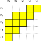
Figure 2. Initial-closed graph $H$ and its illustration by diagram

Proposition 2.6.

Let $H$ be an initial-closed graph. Then the following conditions are equivalent:

1. $H$ is Cohen-Macaulay (i.e. $\operatorname{pd}(H)=n-1$),

2. $H$ is unmixed,

3. $\mu(H)=(0,\ldots,0)$,

4. $\operatorname{reg}(H)=1$.

Proof.

(1) $\Rightarrow$ (2) is well-known.

(2) $\Rightarrow$ (3): We have $H$ is a connected bipartite graph with bipartition $(X,Y)$, where $X=\{x_{1},\ldots,x_{n-1}\}$ and $Y=\{y_{1},\ldots,y_{n-1}\}$. Since $H$ is an initial-closed graph, $H$ satisfies two following conditions:

(a) $$x_{i}y_{i}\in E(H)\text{ for all }1\leq i\leq n-1,$$

(b) $$\text{If }x_{i}y_{j}\in E(H),\text{ then }i\leq j.$$

By Lemma 1.1(1) and Lemma 1.3(1), we assume $N_{H}(x_{1})=\{y_{1},\ldots,y_{t}\}$. If $t<n-1$, then $\{x_{t},y_{t+1}\}\in E(H)$ because $H$ is connected. By [21, Theorem 1.1], $\{x_{1},y_{t+1}\}\in E(H)$, a contradiction. Hence $t=n-1$ which implies $\mu_{1}=0$. By Lemma 1.2, $\mu_{i}=0$ for all $1\leq i\leq n-1$.

(3) $\Rightarrow$ (4): In this case $H$ is a Ferrers graph with $\lambda(H)=(n-1,\ldots,1)$. By [6, Corollary 2.2], $\operatorname{reg}(H)=1$.

(4) $\Rightarrow$ (1): By [12, Theorem 2.2], $\operatorname{reg}(H)=\operatorname{im}(H)=1$. Hence, $H$ is a Ferrers graph with $\lambda(H)=(n-1,\ldots,2,1)$. Thus the assertion follows from [6, Corollary 2.8]. ∎

From now, we will consider the initial-closed graph $H$ with an associated vector $\mu(H)=(\mu_{1},\ldots,\mu_{s},0,\ldots,0)\in\mathbb{N}^{n-1}$, where $0<\mu_{s}\leq\ldots\leq\mu_{1}$, $1\leq s\leq n-3$, and $\mu_{j}\leq n-2-j$ for all $j=1,\ldots,s$.

Lemma 2.7.

Let $H$ be an initial-closed graph. Then

1. If $s=1$, then $\operatorname{pd}(H)=2(n-1)-(\mu_{1}+1),$

2. If $\mu_{1}=\cdots=\mu_{s}=1$, then $\operatorname{pd}(H)=2(n-1)-(s+1).$

Proof.

The assertion (2) is proved similarly as the assertion (1). We now prove assertion (1) by induction on $n$. If $n=4$, then $\mu(H)=(1,0,0)$. In this case, $H$ is a path of length $5$. By [16, Corollary 7.7.35], $\operatorname{pd}(H)=4$.

We now assume that $n\geq 5$. By Lemma 2.4, $H\backslash\{x_{n-1},y_{n-1}\}$ is an initial-closed graph with $\mu(H\backslash\{x_{n-1},y_{n-1}\})=(\mu_{1}-1,0,\ldots,0)\in\mathbb{N}^{n-2}$. By the induction hypothesis, $\operatorname{pd}(H\backslash\{x_{n-1},y_{n-1}\})=2(n-2)-\mu_{1}$. Since $N_{H}(x_{n-1})=\{y_{n-1}\}$, $x_{n-1}$ is an isolated vertex of $H\backslash y_{n-1}$. Thus, $\operatorname{pd}(H\backslash y_{n-1})=\operatorname{pd}(H\backslash\{x_{n-1},y_{n-1}\})=2(n-2)-\mu_{1}.$

By the assumption, $N_{H}(y_{n-1})=\{x_{2},\ldots,x_{n-1}\}$. Hence $\deg_{H}(y_{n-1})=n-2$, and $V(H_{y_{n-1}})=\{x_{1},y_{1},\ldots,y_{n-2}\}$. Thus, $H_{y_{n-1}}$ is the disjoint union of the star graph on vertex set $\{x_{1},y_{1},\ldots,y_{n-1-\mu_{1}}\}$, which apex is $x_{1}$, and the isolated vertices $y_{n-\mu_{1}},\ldots,y_{n-2}$. By [16, Theorem 5.4.11], $\operatorname{pd}(H_{y_{n-1}})=n-1-\mu_{1}$.

By Lemma 2.2(4), we conclude that $\operatorname{pd}(H)=2(n-1)-(\mu_{1}+1)$, as required. ∎

Proposition 2.8.

Let $H$ be an initial-closed graph. If $\mu_{1}=\ldots=\mu_{s}=c\geq 1$, then $\operatorname{pd}(H)=2(n-1)-(c+s).$

Proof.

We prove the lemma by induction on $c$. If $c=1$, then proposition follows from Lemma 2.7(2).

We now assume that $c\geq 2$. By the assumption, $N_{H}(y_{n-1})=\{x_{s+1},\ldots,x_{n-1}\}$. Hence $\deg_{H}(y_{n-1})=n-s-1$ and $V(H_{y_{n-1}})=\{x_{1},\ldots,x_{s}\}\cup\{y_{1},\ldots,y_{n-2}\}$. Thus, $H_{y_{n-1}}$ is the disjoint union of the isolated vertices $y_{n-c},\ldots,y_{n-2}$, and the induced graph $H^{\prime}$ of $H$ on vertex set $\{x_{1},\ldots,x_{s}\}\cup\{y_{1},\ldots,y_{n-c-1}\}$. Note that $H^{\prime}$ is a Ferrers graph with $\lambda(H^{\prime})=(n-c-1,n-c-2,\ldots,n-c-s)\in\mathbb{N}^{s}$. By Lemma 2.3, $\operatorname{pd}(H^{\prime})=n-c-1$, and so $\operatorname{pd}(H_{y_{n-1}})=n-c-1$.

On the other hand, by Lemma 2.4, $H\backslash\{x_{n-1},y_{n-1}\}$ is also an initial-closed graph with $\mu(H\backslash\{x_{n-1},y_{n-1}\})=(c-1,\ldots,c-1,0,\ldots,0)\in\mathbb{N}^{n-2}$. By the induction hypothesis, we have $\operatorname{pd}(H\backslash\{x_{n-1},y_{n-1}\})=2(n-2)-(c-1+s)$. Since $x_{n-1}$ is an isolated vertex of $H\backslash y_{n-1}$, we obtain $\operatorname{pd}(H\backslash y_{n-1})=\operatorname{pd}(H\backslash\{x_{n-1},y_{n-1}\})=2n-3-(c+s).$

By Lemma 2.2(4), we conclude that $\operatorname{pd}(H)=2(n-1)-(c+s).$ ∎

Lemma 2.9.

Let $H$ be an initial-closed graph. If $s\geq 2$, then

$$\operatorname{pd}(H_{x_{s}})=n-1-s+\operatorname{pd}(H^{\prime}),$$

where $H^{\prime}$ is the induced graph of $H$ on the vertex set $\{x_{1},\ldots,x_{s-1}\}\cup\{y_{1},\ldots,y_{s-1}\}$. Moreover $H^{\prime}$ is an initial-closed graph and $\mu(H^{\prime})=(\mu^{\prime}_{1},\ldots,\mu^{\prime}_{s-3},0,0)$ with $\mu^{\prime}_{j}=\max\{0,\mu_{j}-(n-s)\}$ for $1\leq j\leq s-3$. In particular, $\operatorname{pd}(H_{x_{s}})\geq n-2$, and the equality holds if and only if $\mu_{1}\leq n-s$.

Proof.

By the assumption, $N_{H}(x_{s})=\{y_{s},\ldots,y_{n-\mu_{s}-1}\}$, and so $H_{x_{s}}$ is the disjoint union of two subgraphs $H^{\prime}$ and $H^{\prime\prime}$, where $H^{\prime}$ (resp. $H^{\prime\prime}$) is an induced subgraph of $H$ on vertex set $\{x_{1},\ldots,x_{s-1},y_{1},\ldots,y_{s-1}\}$ (resp. $\{x_{s+1},\ldots,x_{n-1},y_{n-\mu_{s}},\ldots,y_{n-1}\}$). Then we get

$$\operatorname{pd}(H_{x_{s}})=\operatorname{pd}(H^{\prime})+\operatorname{pd}(H^{\prime\prime}).$$

We know that $H^{\prime\prime}$ is a Ferrers graph with $\lambda(H^{\prime\prime})=(\lambda^{\prime\prime}_{1},\ldots,\lambda^{\prime\prime}_{n-s-1})$, where $\lambda_{j}^{\prime\prime}:=\deg_{H^{\prime\prime}}(x_{s+j})$ and $\lambda^{\prime\prime}_{j}=\min\{\mu_{s},n-s-j\}$ for $1\leq j\leq n-s-1$. By Lemma 2.3, we get $\operatorname{pd}(H^{\prime\prime})=\max_{1\leq j\leq n-s-1}\{\lambda_{j}^{\prime\prime}+j-1\}=n-s-1.$ In fact, we always have $\operatorname{pd}(H^{\prime\prime})=\max\{n-s-1,\max_{1\leq j\leq n-s-2}\{\lambda^{\prime\prime}_{j}+j-1\}\}.$ Since $\lambda_{j}^{\prime\prime}+j-1=\min\{\mu_{s},n-s-j\}+j-1\leq n-s-1$ for all $1\leq j\leq n-s-1$. Thus, $\operatorname{pd}(H^{\prime\prime})=n-s-1$.

Moreover, by Lemma 2.4, $H^{\prime}$ is also an initial-closed graph with $\mu(H^{\prime})=(\mu_{1}^{\prime},\ldots,\mu_{s-1}^{\prime})$, where $\mu^{\prime}_{j}=\max\{0,\mu_{j}-(n-s)\}$ for all $1\leq j\leq s-1$. Furthermore, we obtain $\mu_{1}^{\prime}\geq\cdots\geq\mu_{s-3}^{\prime}\geq\mu_{s-2}^{\prime}=\mu_{s-1}^{\prime}=0$.

We now prove the last assertion. We always have $\operatorname{pd}(H^{\prime})\geq s-1$, and thus $\operatorname{pd}(H_{x_{s}})\geq n-2$. The equality holds if and only if $\operatorname{pd}(H^{\prime})=s-1$. From Proposition 2.6, $H^{\prime}$ is a Cohen-Macaulay graph. By Proposition 2.6, $\mu(H^{\prime})=(0,\ldots,0)$. It means that $\mu_{1}\leq n-s$. ∎

Lemma 2.10.

Let $H$ be an initial-closed graph. If $s\geq 2$ and $\mu_{1}<n-s$, then

$$\operatorname{pd}(H\backslash x_{s})=\begin{cases}n-1,&\text{ if }\mu_{1}=\ldots=\mu_{s-1}=n-s-1\\ 1+\operatorname{pd}(H\backslash\{x_{s},y_{s}\}),&\text{ otherwise. }\end{cases}$$

Proof.

Let $K:=H\backslash x_{s}$. In order to prove this lemma, we divide the proof in two following cases:

Case 1: $\mu_{s-1}=n-s-1$. We have $\mu_{s-1}\leq\ldots\leq\mu_{1}<n-s$, and so $\mu_{1}=\ldots=\mu_{s-1}=n-s-1$. Hence $K$ is the disjoint union of two Ferrers graphs $H^{\prime}$ and $H^{\prime\prime}$, where $H^{\prime}$ (resp. $H^{\prime\prime}$) is the induced subgraph of $H$ on $\{x_{1},\ldots,x_{s-1},y_{1},\ldots,y_{s}\}$ (resp. $\{x_{s+1},\ldots,x_{n-1},y_{s+1},\ldots,y_{n-1}\}$) with $\lambda(H^{\prime})=(s,\ldots,2)\in\mathbb{N}^{s-1}$ (resp. $\lambda(H^{\prime\prime})=(n-s-1,\ldots,1)\in\mathbb{N}^{n-s-1}$). By Lemma 2.3, we obtain

$$\operatorname{pd}(K)=\operatorname{pd}(H^{\prime})+\operatorname{pd}(H^{\prime\prime})=s+(n-s-1)=n-1.$$

Case 2: $\mu_{s-1}<n-s-1$. Thus, $H\backslash\{x_{s},y_{s}\}$ is connected, and by Lemma 2.4, $H\backslash\{x_{s},y_{s}\}$ is also an initial-closed graph. Note that $K\backslash y_{s}=H\backslash\{x_{s},y_{s}\}$. Since $s\geq 2$ and $\mu_{1}<n-s$, so $\mu(K\backslash y_{s})=(\mu_{1},\ldots,\mu_{s-1},0,\ldots,0)\in\mathbb{N}^{n-2}$. By Proposition 2.6, $K\backslash y_{s}$ is not Cohen-Macaulay. Hence $\operatorname{pd}(K\backslash y_{s})>n-2$.

Moreover, since $\mu_{1}<n-s$, $N_{K}(y_{s})=\{x_{1},\ldots,x_{s-1}\}$ and so $\deg_{K}(y_{s})=s-1$. Then $K_{y_{s}}$ is the union of the isolated vertices $y_{1},\ldots,y_{s-1}$ and a graph $K^{\prime}$, where $K^{\prime}$ is the induced subgraph of $H$ on vertex set $\{x_{s+1},\ldots,x_{n-1},y_{s+1},\ldots,y_{n-1}\}$. Since $H$ is an initial-closed graph, $K^{\prime}$ is also an initial-closed graph with $\mu(K^{\prime})=(0,\ldots,0)\in\mathbb{N}^{n-s-1}$. By Proposition 2.6, $K^{\prime}$ is Cohen-Macaulay and thus $\operatorname{pd}(K^{\prime})=n-s-1$. Therefore, $\operatorname{pd}(K_{y_{s}})=\operatorname{pd}(K^{\prime})=n-s-1$.

By Lemma 2.2(5), $\operatorname{pd}(K)=1+\operatorname{pd}(K\backslash y_{s})$. On the other hand, $\operatorname{pd}(H\backslash x_{s})=1+\operatorname{pd}(H\backslash\{x_{s},y_{s}\})$, which completes the proof of this lemma. ∎

Theorem 2.11.

Let $H$ be an initial-closed graph. If $\mu_{1}<n-s$, then

$$\operatorname{pd}(H)\leq\max_{1\leq j\leq s}\{2(n-1)-(\mu_{j}+j)\}.$$

In particular, if $\mu_{s}<\ldots<\mu_{1}<n-s$, then $\operatorname{pd}(H)=2(n-1)-(\mu_{s}+s)$.

Proof.

We prove by induction on $s$. If $s=1$, by Proposition 2.8, $\operatorname{pd}(H)=2(n-1)-(\mu_{1}+1)$. Now we assume that $s\geq 2$. From Lemma 2.9 and the assumption, $\operatorname{pd}(H_{x_{s}})=n-2$. Note that $N_{H}(x_{s})=\{y_{s},\ldots,y_{n-1-\mu_{s}}\}$, and so $\deg_{H}(x_{s})=n-\mu_{s}-s$.

Next we consider two following cases:

Case 1: $\mu_{s-1}=n-s-1$. By the assumption, $\mu_{1}=\ldots=\mu_{s-1}=n-s-1$. From Lemma 2.10, we have $\operatorname{pd}(H\backslash x_{s})=n-1$. Hence, by Lemma 2.2(2), we have $\operatorname{pd}(H)\leq\max\{2(n-1)-(\mu_{s}+s),n\}=2(n-1)-(\mu_{s}+s)\leq\max_{1\leq j\leq s}\{2(n-1)-(\mu_{j}+j)\}.$

Case 2: $\mu_{s-1}<n-s-1$. By Lemma 2.10, $\operatorname{pd}(H\backslash x_{s})=1+\operatorname{pd}(H\backslash\{x_{s},y_{s}\})$, and $H\backslash\{x_{s},y_{s}\}$ is also an initial-closed graph with $\mu(H\backslash\{x_{s},y_{s}\})=(\mu_{1},\ldots,\mu_{s-1},0,\ldots,0)\in\mathbb{N}^{n-2}$. By the induction hypothesis, $\operatorname{pd}(H\backslash\{x_{s},y_{s}\})\leq\max_{1\leq j\leq s-1}\{2(n-2)-(\mu_{j}+j)\}.$ From Lemma 2.2(2), we have $\operatorname{pd}(H)\leq\max\{2(n-1)-(\mu_{s}+s),\max_{1\leq j\leq s-1}\{2(n-2)-(\mu_{j}+j)\}+2\}=\max_{1\leq j\leq s}\{2(n-1)-(\mu_{j}+j)\}.$

We shall now prove the last statement of this theorem. Assume $\mu_{s}<\ldots<\mu_{1}<n-s$. Then $\mu_{s}+s\leq\ldots\leq\mu_{1}+1$, and so $\max_{1\leq j\leq s}\{2(n-1)-(\mu_{j}+j)\}=2(n-2)-(\mu_{s}+s)$. From Lemma 2.10 and the above assertion, we have

$$\operatorname{pd}(H\backslash x_{s}) = 1+\operatorname{pd}(H\backslash\{x_{s},y_{s}\})$$

$$\leq 1+\max_{1\leq j\leq s-1}\{2(n-2)-(\mu_{j}+j)\}=1+2(n-2)-(\mu_{s-1}+(s-1))$$

$$\leq -1+2(n-1)-(\mu_{s}+s)=-1+\operatorname{pd}(H_{x_{s}})+\deg_{H}(x_{s}).$$

By Lemma 2.2(4), $\operatorname{pd}(H)=2(n-1)-(\mu_{s}+s)$, and the proof of theorem is complete. ∎

3. Lower bound for projective dimension

The purpose of this section is to calculate Betti numbers of initial-closed graphs $H$, so that we give an algorithm (see Algorithm 3.2) using the biadjacency matrix of $H$. This algorithm is distinct to the algorithm given in [18, section 2.4]. With this algorithm, we can obtain in some cases an explicit formula for the projective dimension of $R/I(H)$ in despite of the algorithm in [18], where the formula obtained for the projective dimension is not explicit as in [18, Proposition 2.26].

Let $G$ be a bipartite graph with bipartition $\{x_{1},\ldots,x_{n}\}\cup\{y_{1},\ldots,y_{m}\}$. The biadjacency matrix of $G$, $M(G)=(a_{i,j})\in\mathcal{M}_{n,m}(\{0,1\})$, is defined by $a_{i,j}=1$ if $\{x_{i},y_{j}\}\in E(G)$, 0 otherwise.

Lemma 3.1.

([13, Lemma 1.6]) Let $G$ be a bipartite graph, biadjacency matrix $M=M(G)=(a_{i,j})\in\mathcal{M}_{n,m}(\{0,1\})$.

1. If $M$ has a row or a column whose entries are all $0$, then $\widetilde{H}_{i}(\Delta(G);\Bbbk)={\bf 0}$ for all $i\geq 0$.

2. If there exists $r$ and $c$ such that $a_{r,c}=1$ and the rest of entries on the row $r$ and the column $c$ are zeros, $\widetilde{H}_{i}(\Delta(G);\Bbbk)\cong\widetilde{H}_{i-1}(\Delta(G\backslash\{x_{r},y_{c}\});\Bbbk)$, for all $i>0$.

3. If $M$ has two rows $r$ and $r^{\prime}$ (resp. two columns $c$ and $c^{\prime}$) such that $\{j:a_{r,j}=0\}\subset\{j:a_{r^{\prime},j}=0\}$ (resp. $\{i:a_{i,c}=0\}\subset\{j:a_{i,c^{\prime}}=0\}$), then $\widetilde{H}_{i}(\Delta(G);\Bbbk)=\widetilde{H}_{i}(\Delta(G\backslash x_{r});\Bbbk)\text{ (resp. $\widetilde{H}_{i}(\Delta(G);\Bbbk)=\widetilde{H}_{i}(\Delta(G\backslash y_{c});\Bbbk)$)},$ for all $i\geq 0$.

Let $H$ be a bipartite graph with bipartition $\{x_{1},\ldots,x_{n}\}\cup\{y_{1},\ldots,y_{m}\}$. Let $\lambda=(\lambda_{1},\ldots,\lambda_{n})$ be a partition and let $\mu=(\mu_{1},\ldots,\mu_{n})$ be a vector such that $\mu_{1}\geq\ldots\geq\mu_{n}\geq 0$, $\mu_{i}\leq\lambda_{i}$ for all $1\leq i\leq n$, and $\lambda_{1}=m$. Then we call $H$ skew Ferrers graph if its edge ideal is

$$I(H)=(x_{i}y_{m-\mu_{i}},\ldots,x_{i}y_{m-\lambda_{i}+1}\mid 1\leq i\leq n).$$

The skew Ferrers graphs have a long tradition in combinatorics according to skew Ferrers diagrams, see for example [9, 17]. Note that if $m=n$, $\mu_{i}\leq n-1-i$ for $1\leq i\leq n-2$, $\mu_{n-1}=\mu_{n}=0$ and $\lambda_{i}=n+1-i$ for all $i$, then $H$ is an initial-closed graph. If $\mu_{i}=0$ for all $i$, then $H$ is a Ferrers graph.

Algorithm 3.2.

Input: Let $H$ be a skew Ferrers graph.
Output: An induced matching $U$ of $H$, and a subset $S$ of $V(H)$ such that $\widetilde{H}_{i}(\Delta(H);\Bbbk)={\bf 0}\text{ if }S\neq\emptyset$, and

$$\widetilde{H}_{i}(\Delta(H\backslash S);\Bbbk)\cong\begin{cases}\Bbbk&\text{ if }i=|U|-1\\ {\bf 0}&\text{otherwise.}\end{cases}$$

Let $U:=\emptyset$ and $S:=\emptyset$.

while $H\neq\emptyset$ do

       We assume bipartition of $H$ is $\{x_{i_{1}},\ldots,x_{i_{u}}\}\cup\{y_{j_{1}},\ldots,y_{j_{v}}\}$, where $i_{1}<\ldots<i_{u},$ and $j_{1}<\ldots<j_{v}$;

       $U:=U\cup\{\{x_{i_{u}},y_{j_{v}}\}\}$;

       $S:=S\cup\{y_{j}\in V(H\backslash N_{H}(\{x_{i_{u}},y_{j_{v}}\}))\mid$ the columm with labelling $y_{j}$ in $M(H\backslash N_{H}(\{x_{i_{u}},y_{j_{v}}\}))$ is zero};

       $H:=H\backslash(S\cup N_{H}(\{x_{i_{u}},y_{j_{v}}\}))$;

      

end while

return($U,S$)

Proof.

For each loop of the algorithm, we claim that

(1) $$\widetilde{H}_{i}(\Delta(H);\Bbbk) \cong \widetilde{H}_{i-1}(\Delta(H\backslash N_{H}(\{x_{i_{u}},y_{j_{v}}\}));\Bbbk),$$

(2) $$\widetilde{H}_{i}(\Delta(H\backslash S);\Bbbk) \cong \widetilde{H}_{i-1}(\Delta(H\backslash(S\cup N_{H}(\{x_{i_{u}},y_{j_{v}}\})));\Bbbk).$$

Indeed, let $\alpha\in N_{H}(\{x_{i_{u}},y_{j_{v}}\})\backslash\{x_{i_{u}},y_{j_{v}}\}$, and so $\alpha=x_{r}$ or $\alpha=y_{c}$ for some $r\neq i_{u}$ and $c\neq j_{v}$. Without loss of generality, we may assume $\alpha=x_{r}$, where $r\neq i_{u}$. Since $H$ is a skew Ferrers graph, $\{j\mid a_{r,j}=0\}\subseteq\{j\mid a_{i_{u},j}=0\}$. By Lemma 3.1(3), we have $\widetilde{H}_{i}(\Delta(H);\Bbbk)\cong\widetilde{H}_{i}(\Delta(H\backslash x_{r});\Bbbk).$ Repeating this process for all $\alpha\in N_{H}(\{x_{i_{u}},y_{j_{v}}\})\backslash\{x_{i_{u}},y_{j_{v}}\}$, we obtain

$$\widetilde{H}_{i}(\Delta(H);\Bbbk)\cong\widetilde{H}_{i}(\Delta(H\backslash(N_{H}(\{x_{i_{u}},y_{j_{v}}\})\backslash\{x_{i_{u}},y_{j_{v}}\}));\Bbbk).$$

By Lemma 3.1(2), $\widetilde{H}_{i}(\Delta(H);\Bbbk)\cong\widetilde{H}_{i-1}(\Delta(H\backslash N_{H}(\{x_{i_{u}},y_{j_{v}}\}));\Bbbk)$, as the first assertion.

Let $U:=\{x_{i_{u}},y_{j_{v}}\}$, and $S$ be a set containing $y_{j}\in V(H\backslash N_{H}(\{x_{i_{u}},y_{j_{v}}\}))$ such that the columm with labelling $y_{j}$ in $M(H\backslash N_{H}(\{x_{i_{u}},y_{j_{v}}\}))$ is zero. Note that if $S\neq\emptyset$, then by Lemma 3.1(1) and equality (1), $\widetilde{H}_{i}(\Delta(H);\Bbbk)=0$. Furthermore, $\widetilde{H}_{i}(\Delta(H\backslash S);\Bbbk)\cong\widetilde{H}_{i-1}(\Delta(H\backslash(S\cup N_{H}(\{x_{i_{u}},y_{j_{v}}\})));\Bbbk)$, which completes the proof of the second claim.

Repeating the above loop $|U|$ times, by equality (1), $\widetilde{H}_{i}(\Delta(H);\Bbbk)=0$ if $S\neq\emptyset$; and furthermore by equality (2) we have

$$\widetilde{H}_{i}(\Delta(H\backslash S);\Bbbk)\cong\cdots\cong\widetilde{H}_{i-|U|}(\{\emptyset\};\Bbbk)=\begin{cases}\Bbbk&\text{ if }i=|U|-1\\ {\bf 0}&\text{otherwise.}\end{cases}$$

∎

Remark 3.3.

When we apply this algorithm to a skew Ferrers graph $H$ and using Hochster formula we get $\beta_{i,j}(H)$ is independent on the base field for all $i,j$. This result was obtained also by Nagel and Reiner in [18, Corollary 2.16].

Let $H$ be a skew Ferrers graph. By Algorithm 3.2, the edge set of $H$ can be partitioned into subsets as follows: $E(H)=\bigcup_{e\in U}E_{e},$ where $E_{\{x_{i},y_{j}\}}=\{\{x_{k},y_{l}\}\in E(H)\mid k\leq i,l\leq j,\text{ and }\{x_{k},y_{l}\}\cap N_{H}(\{x_{i},y_{j}\})\neq\emptyset\}$. This partition is called rectangular decomposition, which is similar to the rectangular decomposition given in [18, Section 2.4].

Example 3.4.

A skew Ferrers diagram in Figure 3 with $\mu=(4,2,1,1,0,0)$ and $\lambda=(6,5,4,4,2,1)$. Applying Algorithm 3.2, $U=\{\{x_{6},y_{6}\},\{x_{4},y_{5}\},\{x_{2},y_{2}\}\}$ and $S=\{y_{1}\}$. Then $E_{\{x_{2},y_{2}\}}=\{\{x_{1},y_{1}\},\{x_{1},y_{2}\},\{x_{2},y_{2}\}\}$, $E_{\{x_{6},y_{6}\}}=\{\{x_{5},y_{5}\},\{x_{5},y_{6}\},\{x_{6},y_{6}\}\}$, and $E_{\{x_{4},y_{5}\}}=\{\{x_{2},y_{3}\},\{x_{2},y_{4}\},\{x_{3},y_{3}\},\{x_{3},y_{4}\},\{x_{3},y_{5}\},\{x_{4},y_{3}\},\{x_{4},y_{4}\},\{x_{4},y_{5}\}\}$.

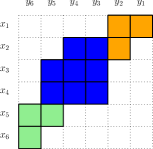
Figure 3. Rectangular decomposition of a skew Ferrers diagram

Lemma 3.5.

If $e\in U$, then $\operatorname{im}(H[E_{e}])=1$.

Proof.

Let $e=\{x_{i},y_{j}\}$. Assume on the contrary that there are two edges $e_{1}:=\{x_{u_{1}},y_{v_{1}}\}$ and $e_{2}:=\{x_{u_{2}},y_{v_{2}}\}$ in $E_{e}$ such that $\{e_{1},e_{2}\}$ is an induced matching of $H$. Then $u_{1}\neq u_{2}$ and $v_{1}\neq v_{2}$. Without loss of generality, we assume $u_{1}<u_{2}$. Since $e_{1},e_{2}\in E_{e}$, so $u_{1}<u_{2}\leq i$, $v_{1},v_{2}\leq j$, $\{x_{u_{1}},y_{v_{1}}\}\cap N_{H}(\{x_{i},y_{j}\})\neq\emptyset$ and $\{x_{u_{2}},y_{v_{2}}\}\cap N_{H}(\{x_{i},y_{j}\})\neq\emptyset$. In order to prove this lemma we divided the proof in two following cases:

Case 1. $x_{u_{1}},x_{u_{2}}\in N_{H}(y_{j})$; or $y_{v_{1}},y_{v_{2}}\in N_{H}(x_{i})$. We will prove for the case $y_{v_{1}},y_{v_{2}}\in N_{H}(x_{i})$, the remain case will be proved similarly. Since $\{x_{i},y_{v_{1}}\}$ and $\{x_{u_{1}},y_{v_{1}}\}$ are two edges of $H$, by Lemmas 1.1(1) and 1.3(1), $\{x_{u_{1}},x_{u_{1}+1},\ldots,x_{i}\}\subseteq N_{H}(y_{v_{1}})$. Thus $\{x_{u_{2}},y_{v_{1}}\}\in E(H)$, a contradiction.

Case 2. $x_{u_{1}}\in N_{H}(y_{j}),y_{v_{2}}\in N_{H}(x_{i})$; or $x_{u_{2}}\in N_{H}(y_{j}),y_{v_{1}}\in N_{H}(x_{i})$. We will prove for the first case, and the remain case will be proved similarly. If $v_{2}<v_{1}$, then $\{x_{u_{2}},y_{v_{1}}\}\in E(H)$ because $\mu_{u_{2}}\leq\mu_{u_{1}}$. It implies that $\{e_{1},e_{2}\}$ is not an induced matching of $H$, a contradiction. Therefore, $v_{2}>v_{1}$, and thus in this case $v_{1}<v_{2}\leq j$. Recall $\{x_{u_{1}},y_{v_{1}}\},\{x_{u_{1}},y_{j}\}\in E(H)$. By Lemmas 1.1(1) and 1.3(1), $\{y_{v_{1}},y_{v_{1}+1},\ldots,y_{j}\}\subseteq N_{H}(x_{u_{1}})$, and so $\{x_{u_{1}},y_{v_{2}}\}\in E(H)$, a contradiction. ∎

Applying the Algorithm 3.2 for an initial-closed graph $H$, we get

Theorem 3.6.

Let $H$ be an initial-closed graph. Then

$$\beta_{2(n-1)-|U|-|S|,2(n-1)-|S|}(H)\neq 0.$$

In particular, $\operatorname{reg}(H)=\operatorname{im}(H)=|U|$, and $\operatorname{pd}(H)\geq 2(n-1)-(|U|+|S|)$.

Proof.

Since $|V(H)\backslash S|=2(n-1)-|S|$, by Hochster formula, we have

$$\beta_{2(n-1)-|U|-|S|,2(n-1)-|S|}(H)\geq\dim_{\Bbbk}\widetilde{H}_{|U|-1}(\Delta(H\backslash S),\Bbbk)=1.$$

Thus, $\operatorname{pd}(H)\geq 2(n-1)-|U|-|S|$.

We claim that $\operatorname{im}(H)=|U|$. Indeed, if $U$ is not a maximum induced matching of $H$, then there is an induced matching $U^{\prime}$ such that $|U^{\prime}|>|U|$. Then by Pigenhole principle, there are at least two edges $e,e^{\prime}$ in $U^{\prime}$ belonging to $E_{e_{i}}$ for some $i$, but this fact contradicts Lemma 3.5, as claimed. So $\operatorname{im}(H)\leq\operatorname{reg}(H)$.

Therefore, by the definition of regularity, we have $\operatorname{im}(H)\leq\operatorname{reg}(H)$. Conversely, in order to prove $\operatorname{im}(H)\geq\operatorname{reg}(H)$, we let $r:=\operatorname{reg}(H)$. Then there exists $i$ such that $\beta_{i,i+r}(H)\neq 0$. By Hochster formula, there is a subset $W\subseteq V(H)$ such that $|W|=i+r$ and $\dim_{\Bbbk}\widetilde{H}_{r-1}(\Delta(H[W]);\Bbbk)\neq 0$. Note that $H[W]$ is a skew Ferrers graph. Applying the Algorithm 3.2 for $H[W]$, there is an induced matching $U_{W}$ of $H[W]$ such that $\dim_{\Bbbk}\widetilde{H}_{r-1}(\Delta(H[W]);\Bbbk)=1$, and $r-1=|U_{W}|-1$. Therefore, $\operatorname{reg}(H)=|U_{W}|\leq\operatorname{im}(H)$. We conclude that $\operatorname{reg}(H)=\operatorname{im}(H)=|U|$. ∎

Remark 3.7.

The equality $\operatorname{reg}(H)=\operatorname{im}(H)$ could be obtained also using [12, Corollary 2.4].

Corollary 3.8.

Let $H$ is an initial-closed graph. If $0<\mu_{s}=\ldots=\mu_{1}$, then $\beta_{2(n-1)-(\mu_{1}+s),2(n-1)-(\mu_{1}+s)+2}(H)$ is the unique extremal Betti number.

Proof.

By Algorithm 3.2, we have $S=\{y_{1},\ldots,y_{s-1},y_{n-\mu_{1}},\ldots,y_{n-2}\}$, and

$$U=\{\{x_{s},y_{n-1-\mu_{1}}\},\{x_{n-1},y_{n-1}\}\}.$$

Thus, by Theorem 3.6, $\operatorname{reg}(H)=2$ and $\beta_{p,p+2}(H)\neq 0$, where $p:=2(n-1)-(\mu_{1}+s)$. Furthermore, by Proposition 2.8, $\operatorname{pd}(H)=p$. Therefore, $\beta_{p,p+2}(H)$ is the unique extremal Betti number. ∎

Corollary 3.9.

Let $H$ is an initial-closed graph. If $0<\mu_{s}<\ldots<\mu_{1}<n-s$, then $\beta_{2(n-1)-(\mu_{s}+s),2(n-1)-(\mu_{s}+s)+3}(H)$ is the unique extremal Betti number.

Proof.

By Algorithm 3.2, we have $S=\{y_{1},\ldots,y_{s-2},y_{n-\mu_{s}},\ldots,y_{n-2}\}$ and

$$U=\{\{x_{s-1},y_{s-1}\},\{x_{s},y_{n-1-\mu_{s}}\},\{x_{n-1},y_{n-1}\}\}.$$

By Theorem 3.6, $\operatorname{reg}(H)=3$ and $\beta_{p,p+3}(H)\neq 0$, where $p:=2(n-1)-(\mu_{s}+s)$. Therefore, the corollary follows from by Theorem 2.11. ∎

Question 1. If $H$ is an initial-closed graph, then does $R/I(H)$ have the unique extremal Betti number?

4. Extremal Betti numbers of closed graphs

We obtain here a partial answer of Ene, Herzog and Hibi conjecture [11] in Theorem 4.2.

Lemma 4.1.

Let $G$ be a connected closed graph without cut point, $\mu(G)=(\mu_{1},\ldots,\mu_{n})$ and $s:=\min\{k-1\mid\mu_{k}=0\}$. Let $R:=\Bbbk[x_{i},y_{i}\mid i\in V(G)]$. If one of three following conditions is satisfied:

1. $s=0$, or

2. $0<\mu_{s}=\ldots=\mu_{1}$, or

3. $0<\mu_{s}<\ldots<\mu_{1}<n-s$,

then $R/\operatorname{in}(J_{G})$ and $R/J_{G}$ have an unique extremal Betti number, and they are equal. In particular, $\operatorname{pd}(R/J_{G})=\operatorname{pd}(R/\operatorname{in}(J_{G}))$ and in the case $s=0$, $\operatorname{pd}(R/\operatorname{in}(J_{G}))=n-1$; and in the remain two cases, $\operatorname{pd}(R/\operatorname{in}(J_{G}))=2n-\mu_{s}-s-2$.

Proof.

Let $H$ be the initial-closed graph associated to $G$, i.e. $I(H)=\operatorname{in}(J_{G})$.

(1) By Proposition 2.6, $\operatorname{reg}(H)=1$ and $\operatorname{pd}(H)=n-1$. We have $R/I(H)$ and $R/\operatorname{in}(J_{G})$ have the same Betti numbers; so $\operatorname{reg}(R/\operatorname{in}(J_{G}))=1$, $\operatorname{pd}(R/\operatorname{in}(J_{G}))=n-1$ and $R/\operatorname{in}(J_{G})$ has an unique extremal Betti number. As $R/\operatorname{in}(J_{G})$ and $R/J_{G}$ have the same Hilbert function, they have the same Betti numbers.

(2) Let $p:=2(n-1)-(\mu_{1}+s)$. By Corollary 3.8, $\beta_{p,p+2}(R/\operatorname{in}(J_{G}))$ is the unique extremal Betti number of $R/\operatorname{in}(J_{G})$. So, $\operatorname{pd}(R/\operatorname{in}(J_{G}))=p$ and $\operatorname{reg}(R/\operatorname{in}(J_{G}))=2$. Since $R/J_{G}$ and $R/\operatorname{in}(J_{G})$ have the same Hilbert function, $\beta_{p,p+2}(R/J_{G})=\beta_{p,p+2}(R/\operatorname{in}(J_{G}))$. Thus $\operatorname{pd}(R/J_{G})=p$ and $\operatorname{reg}(R/J_{G})=2$ and we conclude that $\beta_{p,p+2}(R/J_{G})$ is the unique extremal Betti number of $R/J_{G}$.

(3) Let $p:=2n-\mu_{s}-s-2$. By Corollary 3.9, $\beta_{p,p+3}(R/\operatorname{in}(J_{G}))$ is the unique extremal Betti number of $R/\operatorname{in}(J_{G})$; and we obtain the claim as in (2).

∎

Using Proposition 1.8 and Lemma 4.1 we obtain the following theorem:

Theorem 4.2.

Let $G$ be a connected closed graph with $\ell$ cut points $v_{1},\ldots,v_{\ell}$. Assume that $G=G_{1}\cup\ldots\cup G_{\ell+1}$ such that $G_{i}\cap G_{i+1}=\{v_{i}\}$ and $G_{i}\cap G_{j}=\emptyset$ for $i=1,\ldots,\ell$ and $i\neq j\neq i+1$. Let $n_{i}=|V(G_{i})|$ and $\mu(G_{i})=(\mu_{i1},\ldots,\mu_{in_{i}})$, where $s_{i}:=\min\{k-1\mid\mu_{ik}=0\}$. If for each $i$, one of three following conditions is satisfied:

1. $s_{i}=0$, or

2. $0<\mu_{is_{i}}=\ldots=\mu_{i1}$, or

3. $0<\mu_{is_{i}}<\ldots<\mu_{i1}<n_{i}-s_{i}$;

then $R/\operatorname{in}(J_{G})$ and $R/J_{G}$ have an unique extremal Betti number, and they are equal. In particular, $\operatorname{pd}(R/J_{G})=\operatorname{pd}(R/\operatorname{in}(J_{G}))$.

Remark 4.3.

If Question 1 has an affirmative answer, theorem 4.2 will be true for all closed graph $G$; and thus $\operatorname{reg}(R/J_{G})=\operatorname{reg}(R/\operatorname{in}(J_{G}))$ and $\operatorname{pd}(R/J_{G})=\operatorname{pd}(R/\operatorname{in}(J_{G}))$.

Acknowledgment

This work was finished during the second author’s postdoctoral fellowship at Universidad Nacional Autónoma de Mexico (UNAM) and Universidad Autónoma de Zacatecas (UAZ). He would like to thank UNAM and UAZ for the financial support and hospitality. He is also partially supported by the NAFOSTED (Vietnam) under grant number 101.04-2015.02. The first author would like to thank Luis Manuel Rivera for stimulating discussions.

References

- [1] K. Baclawski and A. M. Grasia, Combinatorial decompositions of a class of rings, Adv. Math. 39 (1981) 155-184.
- [2] A. Banerjee and L. Núñez-Betancourt, Graph connectivity and binomial edge ideals, Proc. Amer. Math. Soc. 145 (2017), 487-499.
- [3] H. Baskoroputro, On the binomial edge ideals of proper interval graphs, arXiv:1611.10117v1 (2016).
- [4] J. A. Bondy and U. S. R. Murty, Graph Theory, no. 244 in Graduate Texts in Mathematics, Springer, 2008.
- [5] F. Chaudhry, A. Dokuyucu and R. Irfan, On the binomial edge ideals of block graphs, An. Stiint. Univ. ”Ovidius” Constanta Ser. Mat. 24 (2016), 149-158.
- [6] A. Corso and U. Nagel, Monomial and toric ideals associated to Ferrers graphs, Trans. Am. Math. Soc. 361(3), (2005) 591-613.
- [7] D. A. Cox and A. Erskine, Closed graph I, Ars Combin. 120 (2015), 259-274.
- [8] H. Dao, C. Huneke, and J. Schweig, Bounds on the regularity and projective dimension of ideals associated to graphs, J. Algebraic Combin. 38 (2013), 37-55.
- [9] M.P. Delest and J.M. Fedou, Enumeration of skew Ferrers diagrams, Discrete Mathematics 112 (1993), 65-79.
- [10] A. Dokuyucu, Extremal Betti numbers of some classes of binomial edge ideals, Math. Rep. 17(4) (2015), 359-367.
- [11] V. Ene, J. Herzog and T. Hibi, Cohen-Macaulay binomial edge ideals, Nagoya Math. J. 204 (2011), 57-68.
- [12] V. Ene and A. Zarojanu, On the regularity of binomial edge ideals, Math. Nachr. 288 (2015), 19-24.
- [13] O. Fernandez and P. Gimenez, Regularity 3 in edge ideals associated to bipartite graphs, J. Algebr Comb. 39 (2014), 919-937.
- [14] J. Herzog and T. Hibi, Monomial ideals. Graduate Texts in Mathematics, 260. Springer-Verlag London, Ltd., London, 2011.
- [15] J. Herzog, T. Hibi, F. Hreinsdottir, T. Kahle, and J. Rauh, Binomial edge ideals and conditional independence statements, Adv. Appl. Math. 45 (2010), 317-333.
- [16] S. Jacques, Betti numbers of graph ideals, University of Sheffield: PhD thesis. math.AC/0410107 (2004).
- [17] I. G. Macdonald, Symmetric functions and Hall polynomials, 2nd edition, Oxford Mathematical Monographs. Oxford Science Publications. The Clarendon Press, Oxford University Press, New York, 1995.
- [18] U. Nagel and V. Reiner, Betti numbers of monomial ideals and shifted skew shapes, Electron. J. Comb. 16 (2) (2009), Special volume in honor of Anders Björner, Research paper 3, pp. 59.
- [19] M. Ohtani, Graphs and Ideals generated by some 2-minors, Comm. Algebra 39 (3) (2011), 905-917.
- [20] P. Schenzel and S. Zafar, Algebraic properties of the binomial edge ideal of a complete bipartite graph, An. Stiint. Univ. ”Ovidius” Constanta Ser. Mat. 22 (2014), 217-237.
- [21] R. H. Villarreal, Monomial Algebras, Monographs and Textbooks in Pure and Applied Mathematics, vol. 238. Marcel Dekker, New York 2001.