On the Renormalization Group perspective of $\alpha$-attractors

Abstract

In this short paper we outline a recipe for the reconstruction of $F(R)$ gravity starting from single field inflationary potentials in the Einstein frame. For simple potentials one can compute the explicit form of $F(R)$, whilst for more involved examples one gets a parametric form of $F(R)$. The $F(R)$ reconstruction algorithm is used to study various examples: power-law $\phi^{n}$, exponential and $\alpha$-attractors. In each case it is seen that for large $R$ (corresponding to large value of inflaton field), $F(R)\sim R^{2}$. For the case of $\alpha$-attractors $F(R)\sim R^{2}$ for all values of inflaton field (for all values of $R$) as $\alpha\to 0$. For generic inflaton potential $V(\phi)$, it is seen that if $V^{\prime}/V\to 0$ (for some $\phi$) then the corresponding $F(R)\sim R^{2}$. We then study $\alpha$-attractors in more detail using non-perturbative renormalisation group methods to analyse the reconstructed $F(R)$. It is seen that $\alpha\to 0$ is an ultraviolet stable fixed point of the renormalisation group trajectories.

I Introduction

Receding galaxies showed for the first time that the universe we live in is expanding. This was one of the first few observation testing the Einstein general-relativity and giving it a fundamental status. This expansion can be beautifully expressed in terms of Freidmann-Lemaitre-Robertson-Walker (FLRW) metric which follows from the Einstein’s equation under the assumption of homogeneity and isotropy. The conformally-flat metric evolution in time is dictated entirely by the flow of its scale-factor. This flow of scale-factor when extended backward in time leads to causally disconnected regions of space-time, clashing with the homogeneity and isotropic thermal nature observed in the CMB, leading to the famous horizon problem. The flatness and monopole problem further intensifies the severity of the incompleteness of the theory in the early universe.

It is seen that these problems gets resolved if an era of exponential expansion existed in the early universe Guth1980 ; Starobinsky1980 ; Linde1981 . An existence of such an exponential era can further explain large-scale structure. The only issue is how can such an era may have started leading to exponential expansion? Investigation of Einstein field equations shows that theoretically either gravity needs to be modified at high-energy or there exist additional matter whose equation of state is such that it leads to exponential expansion Linde1983 . In the former case one needs to modify the gravity action by adding an $R^{2}$-term (or higher-order terms) to Einstein-Hilbert action (where $R$ is the Ricci-scalar of the metric) Starobinsky1982 . Such higher-derivative terms leads to accelerated expansion. In the later case, it is possible to achieve an accelerated phase with a slowly rolling scalar field (also known as inflaton) across a nearly flat potential.

There are many models which are trying to systematically achieve accelerated expansion in the early epoch of the universe and are compatible with the PLANCK survey data Martin2013 . These include single field model, multi-field models, modified gravity, models inspired form strings, etc. However to compares these models with data one needs to reduce them to single field model where the action distinctively has Einstein-Hilbert gravity term and a scalar-field part with kinetic and potential term. It is realised that to achieve successful inflation with roughly $60$ e-folds it is important that the inflationary potential is very flat.

Particularly interesting are $F(R)$ models of gravity Sotiriou2008 ; DeFelice2010 , where Starobinsky inflation falls in a subclass Starobinsky1980 ; Starobinsky1982 . These models in Jordan-frame leads to modified equation of motion for the evolution of scale-factor of universe. Under appropriate choice of parameters it is possible to achieve acceptable accelerated expansion. By conformal transformation this models can be cast in to Einstein-Hilbert gravity coupled minimally with scalar field, where the potential of scalar-field depends on the form of $F(R)$ Maeda1987 ; Barrow1988 . This frame is referred to as Einstein-frame. The potential in this frame can be compared with the PLANCK survey data and appropriately constrained. One can reverse this process and ask about the functional form of $F(R)$ for the various single field inflationary potential. This process is called $F(R)$ reconstruction Rinaldi2014 ; Bamba2014_1 ; Bamba2014_2 ; Pizza2014 ; Broy2014 ; Myrzakulov2015 . In this sense the two approaches to inflation: modified gravity and new matter are related to each other as one can be transformed into another.

An interesting models of inflation are cosmological attractors where the issue with initial conditions gets resolved nicely. A famous cosmological attractor is the $\alpha$-attractors Kallosh2015 ; Linde2015 ; Carrasco2015_1 ; Carrasco2015_2 ; Kallosh2016 ; Linde2016 ; Pinhero2017 (another interesting attractor models are in scalar-tensor theories of gravity Kallosh2013 ; Kallosh2013maa ; Elizalde2015 ; Choudhury2017 ). The model is written with a non-canonical kinetic term along with a potential (which can be arbitrary). Under field redefinition the kinetic piece acquires canonical form and the potential is modified. The model depends on the parameter $\alpha$ (along with set of parameters appearing in potential). The flatness of Einstein-frame potential for large field values (for any $\alpha$) resolve the issues with initial conditions. These kind of $\alpha$-attractor can be naturally embedded in the setting of supergravity to get a well defined consistent model of inflation following from a fundamental theory. Therefore they become favourable models in the context of inflation. Moreover, the inflationary predictions of these models are robust under quantum corrections to the potential Fumagalli2016 . Recently it has been suggested that $\alpha$-attractors may describe dark matter and perhaps even dark energy giving them an even more wider appeal Mishra2017 . The interesting thing in these models is the existence of attractor point $\alpha\to 0$.

The $F(R)$ reconstruction of $\alpha$-attractors has been recently done to see how the corresponding $F(R)$ function behaves for various values of $\alpha$ Odintsov2016 ; Bhattacharya2017 ; Miranda2017 . $F(R)$ reconstruction appears as a simple algorithm to determine the form of $F(R)$ for the given Einstein frame inflationary potential $V(\phi)$. It turns out, as is shown in this paper, that only for simple form of potential one can actually work out the explicit form of $F(R)$, while in all other case one gets the expression in parametric from. In the case of $\alpha$-attractor one arrives at a parametric form of reconstructed $F(R)$, which is used for further study.

The aim of this paper is to study the quantum field theory of $\alpha$-attractors and compute the renormalisation group flows of the parameters present in the theory, to see whether $\alpha=0$ can appear as a stable gaussian fixed point of the RG trajectories. To achieve this we study the RG flows of the reconstructed $F(R)$ via non-perturbative flow equation Wetterich1992 . An interesting insight is gained if one exploits the non-perturbative renormalisation group flows of generic $F(R)$ functions Machado2007 ; Codello2007 ; Codello2008 ; Ohta20151 ; Ohta20152 ; Falls20161 ; Falls20162 , which have been computed using functional renormalisation group equation in the context of asymptotic safety scenario Niedermaier2006 ; Percacci2007 . In this paper we make use of the already computed RG flow of generic $F(R)$ Ohta20151 ; Ohta20152 ; Falls20161 ; Falls20162 to analyse the behaviour of reconstructed $F(R)$ for the case of $\alpha$-attractor. As the fixed point structure and their stability is independent of the field transformation therefore such fixed point analysis will be frame independent. We study $\alpha$-attractor in this setting and compute the beta-function of its parameters from the RG flow of reconstructed $F(R)$. We do the fixed point analysis of the flow equation and see that the model has a UV attractive fixed point at $\alpha=0$ satisfying the norms of asymptotic safety scenario. This adds a welcoming feature to the $\alpha$-attractor model.

The outline of paper is follows: section II describes the algorithm for the reconstruction formalism and show how for a given potential of scalar field in Einstein-frame gives the corresponding $F(R)$. Section III discuss about the RG flows in general and how qualitative properties (like existence of fixed point and eigenvalues) remains unchanged under field transformation. Here we then study the RG flow of reconstructed $F(R)$ for the case of $\alpha$-attractor using the non-perturbative flow equation and perform the fixed point analysis. Finally conclusions are presented in section IV.

II $F(R)$ reconstruction

In this section we will outline the procedure for the reconstruction of $F(R)$ for the given potential $V(\phi)$ in the Einstein frame. We start by considering the transformation of Jordan-frame $F(R)$-gravity action to Einstein-frame via conformal scaling. The $F(R)$-gravity action in Jordan-frame is given by

$$S_{J}=\int{\rm d}^{d}x\sqrt{-g}F(R)\,,$$ (1)

where $g_{\mu\nu}$ is the metric in Jordan-frame while $R$ is the corresponding Ricci scalar . For generality the dimension of space-time is kept arbitrary. Following the standard procedure Maeda1987 ; Barrow1988 , one can write the $F(R)$ action as a scalar-field coupled to gravity. The two theories are related by Legendre transform,

$$S=\int{\rm d}^{d}x\sqrt{-g}\left[F(\psi)+F^{\prime}(\psi)(R-\psi)\right]\,,$$ (2)

where $\psi$ is an auxiliary field whose equation of motion is $\psi=R$. This when plugged back in eq. (2) gives $F(R)$ gravity action. At this point one can do conformal transformation $g_{\mu\nu}=\Omega^{2}\bar{g}_{\mu\nu}$ to relate the Jordan frame metric $g_{\mu\nu}$ with the Einstein frame metric $\bar{g}_{\mu\nu}$. On choosing the scale factor $\Omega(x)$ such that $\Omega^{d-2}F^{\prime}(\psi)=(16\pi G)^{-1}$ is satisfied, then one gets the dual theory in the Einstein-frame. The action of which is given by,

$$S_{E} = \int{\rm d}^{d}x\sqrt{-\bar{g}}\biggl{[}\frac{\bar{R}}{16\pi G}-\frac{1}{2}\partial_{\mu}\phi\partial^{\mu}\phi-V(\phi)\biggr{]}\,,$$ (3)

where $\bar{R}$ is the Ricci scalar of the Einstein frame metric $\bar{g}_{\mu\nu}$ and

$$\frac{\phi}{M^{(d-2)/2}_{p}}=\frac{1}{a}\ln\frac{F^{\prime}(\psi)}{M_{P}^{d-2}}\,,\hskip 8.53581ptV(\phi)=\frac{M_{P}^{d}(\psi F^{\prime}-F)}{(F^{\prime})^{d/(d-2)}}\,,$$ (4)

where $M^{d-2}_{p}=(16\pi G)^{-1}$ is the reduced Planck mass in the $d$-dimensions and $a=\sqrt{(d-2)/(2(d-1))}$. These equations gives the functional form of the potential $V(\phi)$ in the Einstein frame for the given $F(R)$ gravity. But it is interesting to ask whether this process can be reversed, in the sense that for a given potential $V(\phi)$ in the Einstein frame what is the corresponding function $F(R)$? This reverse process is commonly called $F(R)$-reconstruction Rinaldi2014 ; Bamba2014_1 ; Bamba2014_2 ; Pizza2014 ; Broy2014 ; Myrzakulov2015 . It turns out that although this reconstruction recipe sounds like a simple algorithm to implement, in practice it is not always possible to compute the explicit functional form of $F(R)$. In those cases one has to rely on numerical methods or express it in parametric form where both $F$ and $R$ are functions of $\phi$. This complexity arises due to the non-linear coupled differential equations involved in the process. Below we outline the algorithm for the reconstruction process.

We first express $F^{\prime}(\psi)$ in terms of $\phi$ using the first equation in (4). This gives

$$F^{\prime}=M_{P}^{d-2}\exp\left(\frac{a\phi}{M_{P}^{(d-2)/2}}\right)\,.$$ (5)

Taking a derivative of this equation with respect to $\psi$ gives,

$$F^{\prime\prime}=aM_{P}^{(d-2)/2}\exp\left(\frac{a\phi}{M_{P}^{(d-2)/2}}\right)\frac{{\rm d}\phi}{{\rm d}\psi}\,.$$ (6)

Plugging the expression of $F^{\prime}$ from eq. (5) in the equation for $V$ given in eq. (4) and taking the derivative of this residual equation with respect to $\psi$ leads to an expression from which one can extract the relation between $\psi$ and $\phi$. For this one will have to use eq. (6). It should be noted that during the Legendre transform which is given in eq. (2), the equations of motion for $\psi$ give $\psi=R$ (where $R$ is the Ricci scalar of the metric in Jordan frame). This implies that the expression for Jordan frame $R$ in terms of $\phi$ is following,

$$aR=M_{P}^{-(d-2)/2}\exp\left(\frac{2a\phi/(d-2)}{M_{P}^{(d-2)/2}}\right)\left[V^{\prime}(\phi)+\frac{adV(\phi)}{(d-2)M_{P}^{(d-2)/2}}\right]\,.$$ (7)

One can now make use of the second equation in (4), where one can plug the expression for $F^{\prime}$ and $\psi$ from eq. (5) and (7) respectively. This will directly give the expression for $F$ in terms of $\phi$.

$$F(\phi)=\frac{M_{P}^{(d-2)/2}}{a}\exp\left(\frac{da\phi/(d-2)}{M_{P}^{(d-2)/2}}\right)\left[V^{\prime}+\frac{2a}{(d-2)M_{P}^{(d-2)/2}}V\right]\,.$$ (8)

From eq. (7 & 8) it is seen that it is a parametric representation of the reconstructed $F(R)$. In the case when $V$ is simple then it is possible to invert eq. (7) to express $\phi$ in terms of $R$, which is then plugged in eq. (8) to get an explicit form for $F(R)$. However in most case of interests (for inflationary potentials) such an inversion is not possible and an explicit expression for $F(R)$ cannot be given. In those cases one can still write a parametric form and use it for further analysis.

In the following we will work out the functional form of $F(R)$ for some simple inflationary potentials in $d=4$.

II.1 $\phi^{n}$ potential

In this case $V(\phi)=\lambda\phi^{n}$. This is a very simple form of potential with just one term. For this potential the eq. (8) and (7) becomes following,

$$R = \frac{\lambda\phi^{n-1}\exp(\phi/(\sqrt{3}M_{P}))}{M_{P}}\left(n\sqrt{3}+\frac{2\phi}{M_{P}}\right)\,,$$

$$F = \lambda\phi^{n-1}M_{P}\exp(2\phi/(\sqrt{3}M_{P}))\left(n\sqrt{3}+\frac{\phi}{M_{P}}\right)\,.$$ (9)

It is seen that even for this simple potential it is difficult to invert for arbitrary $n$ and express $\phi$ in terms of $R$ without involving complicated functions. However the parametric form is good and contains same information. Specialising for the case of $n=1$ it is realised that in this particular case one can actually write an explicit form for the function $F(R)$ by rescaling $\phi\to\bar{\phi}=(\sqrt{3}+2\phi/M_{P})/2$ and $R\to\bar{R}=(M_{p}\sqrt{e}/(2\lambda\sqrt{3}))R$. Under such a rescaling it is possible to do inversion in the first equation in (II.1) giving,

$$\bar{R}=\bar{\phi}e^{\bar{\phi}}\,.$$ (10)

This is the equation of the Lambert W-function. In terms of Lambert W-function one can then express the functional form for $F(R)$ as

$$F(R)=\frac{M_{P}^{3}R^{2}}{4\lambda\sqrt{3}}\left[\frac{1}{2}\bar{\phi}^{-2}+\bar{\phi}^{-1}\right]\,,$$ (11)

where $\bar{\phi}=W[(M_{P}\sqrt{e}/(2\lambda\sqrt{3}))R]$. For $R\ll(\lambda/M_{p})$ one can do a series expansion of the $F(R)$ function to get,

$$F(R)=\frac{M_{P}}{\sqrt{e}}\biggl{[}2\Lambda+M_{P}R+\frac{M_{P}^{2}R^{2}}{16\Lambda}+\cdots\biggr{]}\,,$$ (12)

where $\Lambda=\lambda/4\sqrt{3e}$. This has a more familiar appearance where the various terms are successive powers of $R$ suppressed by powers of $\Lambda/M_{p}$. The large $\phi$ correspond to large $R$-regime. It is noticed that for large $\phi$ in $n=1$ case, the exponential factor leads over the linear $\phi$ term giving $F(R)\sim R^{2}$.

In the more generic case of arbitrary $n$ it is no longer possible to invert the first equation of (II.1) to express $\phi$ in terms of $R$. One is then left with a parametric form of $F(R)$. In this case again we note that for small ($\phi\ll M_{P}$), we have small $R$. In this regime $F(R)\sim R$. In case of large $R$ ($\phi\gg M_{P}$), one gets $R\sim\lambda\phi^{n}\exp(\phi/(\sqrt{3}M_{P}))$ and $F\sim\lambda\phi^{n}\exp(2\phi/(\sqrt{3}M_{P}))$. Here one can see with some manipulation that $F(R)\sim R^{2}$ for large $R$. Also one can compute the following quantity $d\ln(F)/d\ln(R)$ which gives the rate of variation of $F$ w.r.t. $R$. In the parametric case it is given by,

$$\frac{{\rm d}\ln(F)}{{\rm d}\ln(R)}=\frac{{\rm d}\ln(F)}{{\rm d}\phi}\frac{{\rm d}\phi}{{\rm d}\ln(R)}=\frac{nM_{P}\sqrt{3}+2\phi}{nM_{P}\sqrt{3}+\phi}\,.$$ (13)

From here it is clearly seen that for large $\phi$, the r.h.s. approaches $2$ implying $F\sim R^{2}$. This also signifies the the fact that at high energy (for large $\phi$) one always approaches a $R^{2}$ action of gravity. This is like an attractor behaviour. These findings can be more clearly seen by plotting the parametric reconstructed $F(R)$ as a function of $R$ for various $n$. This is shown in figure 1.

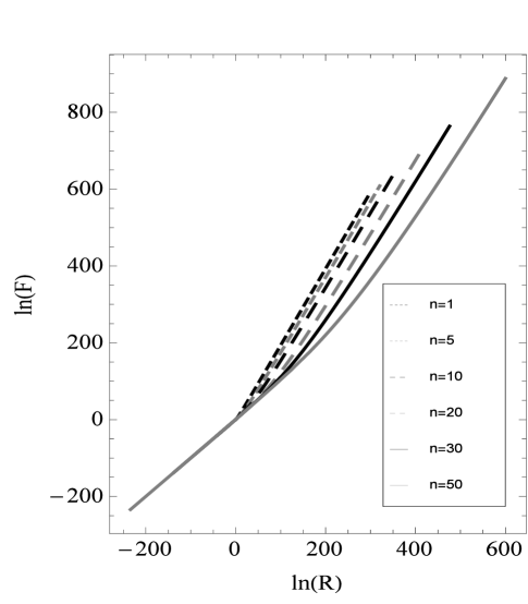
Figure 1: $F(R)$ for $\phi^{n}$. Here on x-axis we plot $\ln(R)$ and on y-axis $\ln(F)$. It is seen that for small $R$ the $F(R)\sim R$, while $F(R)\sim R^{2}$ for large $R$. Here we have kept $M_{P}=1$.

II.2 Exponential potential

The other simple scenario is the case when $V(\phi)$ has an exponential form. Lets say $V(\phi)=\Lambda\exp(b\phi/M_{P})$. Here $\Lambda$ has mass dimension $4$, while $b$ is dimensionless. Then using eq. (7) one can express $\phi$ easily in terms of $\psi$. This is given by,

$$\frac{\phi}{M_{P}}=\frac{\sqrt{3}}{1+b\sqrt{3}}\ln\left(\frac{M_{P}^{2}R}{(2+b\sqrt{3})\Lambda}\right)\,.$$ (14)

Plugging this back in second equation (8) and following the previous foot-steps leads to

$$F(R)=(1+b\sqrt{3})\Lambda\left(\frac{M_{P}^{2}R}{(2+b\sqrt{3})\Lambda}\right)^{(2+b\sqrt{3})/(1+b\sqrt{3})}\,,$$ (15)

In the special case when $b=0$ one gets $R^{2}$ action. If $b=-(n-2)a/(n-1)$, then $F(R)\sim R^{n}$. In the case when $V(\phi)=\Lambda(1-b_{1}\exp(b\phi/M_{P}))^{n}$, it is noticed that

$$R = \frac{\Lambda}{M_{P}^{2}}\exp\left(\frac{\phi}{M_{P}\sqrt{3}}\right)(1-b_{1}\exp(b\phi/M_{P}))^{n-1}[2-b_{1}(nb\sqrt{3}+2)\exp(b\phi/M_{P})]\,,$$ (16)

$$F = \Lambda\exp\left(\frac{2\phi}{M_{P}\sqrt{3}}\right)(1-b_{1}\exp(b\phi/M_{P}))^{n-1}[1-b_{1}(nb\sqrt{3}+1)\exp(b\phi/M_{P})]\,.$$ (17)

Here it is seen that for arbitrary $n$, $b$ and $b_{1}$ it is not possible to do the inversion and express $\phi$ in terms of $R$. But for the special case $b=-2/(n\sqrt{3})$ cancellation in the expression of $R$ occurs which simplifies the expression of $R$. This allows one to do the inversion and express $\phi$ in terms of $R$. Furthermore if $n=2$ the situation simplifies very much and one gets a simple expression for $F(R)$ to be

$$F(R)=M_{P}^{2}\left(b_{1}R+\frac{M_{P}^{2}}{4\Lambda}R^{2}\right)\,.$$ (18)

This is the usual Starobinsky $R^{2}$ model which follows from the reconstruction process.

II.3 $\alpha$-attractor

An interesting case which is quite famous in context of inflation is $\alpha$-attractors. These were first suggested in Kallosh2015 ; Linde2015 ; Carrasco2015_1 ; Carrasco2015_2 which can be easily embedded in supergravity giving it a more fundamental status. Here the action has a non-canonical kinetic term of the scalar field with a $\phi^{2}$ type potential. The action for $T$-models is given by,

$$S_{T}=\int{\rm d}^{4}x\sqrt{-g}\biggl{[}\frac{R}{16\pi G}-\frac{\partial_{\mu}\varphi\partial^{\mu}\varphi}{1-\varphi^{2}/6\alpha}-\frac{m^{2}\varphi^{2}}{2}\biggr{]}\,,$$ (19)

where $m^{2}$ and $\alpha$ are parameters of the theory. Under the field transformation $\varphi=\sqrt{6\alpha}\tanh(\phi/\sqrt{6\alpha})$ the action acquires a canonical kinetic form where the Einstein frame potential is given by,

$$V_{T}(\phi)=3\alpha m^{2}\tanh^{2}\left(\frac{\phi}{\sqrt{6\alpha}}\right)\,.$$ (20)

Another model of $\alpha$-attractors is the $E$-models. Its potential in Einstein frame is,

$$V_{E}(\phi)=3\alpha m^{2}\left(1-e^{-\sqrt{2/(3\alpha)}\phi}\right)^{2}\,.$$ (21)

However in the rest of paper we will study only $T$-models as the results obtained can be easily extended to $E$-models. For $\alpha$-attractors the potential is complicated function of $\phi$, so invertibility during the reconstruction mechanism is not possible. However one can still write the parametric form of $F(R)$ using the eq. (7) and (8). The $\alpha$-attractor has a special point at $\alpha=0$. Each non-zero value of $\alpha$ correspond to an inflationary model and acquires a point on the $n_{s}$-$r$ (where $n_{s}$ is the spectral index and $r$ is the tensor-scalar ratio). When $\alpha\to 0$ smoothly then on the $n_{s}$-$r$ plane the corresponding point is seen to approach smoothly a fixed point, at which $r=0$ and $n_{s}=1-2/N$ (where $N$ is the number of $e$-folds). For small $\alpha$ the model behaves very much like pure $R^{2}$ inflationary model. In fact if one does the reconstruction and plots $F(R)$ for various values of $\alpha$ (see Odintsov2016 ; Bhattacharya2017 ; Miranda2017 for earlier work on $F(R)$ reconstruction of $\alpha$-attractor), then it is seen that for small $\alpha$, $F(R)\sim R^{2}$. If we compute the derivative $d\ln(F)/d\ln(R)$ then it is given by,

$$\frac{{\rm d}\ln(F)}{{\rm d}\ln(R)}=\frac{2\sqrt{2}M_{P}+2\sqrt{\alpha}\sinh(\sqrt{2/3\alpha}\phi)}{2\sqrt{2}M_{P}+\sqrt{\alpha}\sinh(\sqrt{2/3\alpha}\phi)}\,.$$ (22)

Keeping $\alpha$ fixed it is seen that there are two distinct phases: small $\phi$ where $F(R)\sim R$ and large $\phi$ where $F(R)\sim R^{2}$. By varying $\alpha$ it is seen that as $\alpha\to 0$ then this derivative approaches $2$ for all $\phi$, indicating that $\alpha\to 0$ is a $R^{2}$ gravity. These findings can also be inferred by plotting the reconstructed $F(R)$ for the case of $T$-models (for $E$-models it is similar) for various values of $\alpha$ for a range of values of $\phi$. These are presented in figure 2.

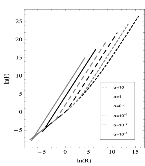
Figure 2: Reconstructed $F(R)$ for $\alpha$-attractor for the $T$-models. Here on x-axis we plot $\ln(R)$ and on y-axis $\ln(F)$. It is seen that for small $R$ the $F(R)\sim R$, while for large $R$ $F(R)\sim R^{2}$. Also as $\alpha$ approaches smaller values, $F\to R^{2}$.

This is good indication of $R^{2}$ being an attractor point at high energies. This classical analysis motivates us to indulge in to investigating whether $\alpha=0$ can be a stable fixed point in the corresponding quantum theory, where $\alpha=0$ arises as the ultraviolet stable fixed point of the renormalisation group trajectory. If such a thing is possible then it gives different perspective to the $\alpha=0$ point. In the next section therefore we will study the quantum theory of the $\alpha$-attractors and compute the RG flow of the coupling parameters.

II.4 Generic $V(\phi)$

In the case when the potential is generic $V(\phi)$ then using eq. (7 & 8) one can write reconstructed $F(R)$. In generic case one can take derivative $d\ln(F)/d\ln(R)$ to see the form of the resulting expression. This is given by,

$$\frac{{\rm d}\ln(F)}{{\rm d}\ln(R)}=\frac{2\sqrt{3}V(\phi)+3M_{P}V^{\prime}(\phi)}{\sqrt{3}V(\phi)+3M_{P}V^{\prime}(\phi)}\,.$$ (23)

This simple expression shows that if $V^{\prime}/V$ vanishes then one gets the derivative to be $2$, indicating $R^{2}$ gravity. For the forms of $V$ considered above it is seen that $V^{\prime}/V$ vanishes for large $\phi$: for polynomial forms of potential, $\alpha$-attractor, power-law. In the case of exponential potential this ratio vanishes only for special value of $b$ (the coefficient appearing the exponential). In case of $\alpha$-attractor this ratio vanishes for all values of $\phi$ as $\alpha\to 0$, giving $R^{2}$ gravity.

III RG flows

As the point $\alpha\to 0$ hold a special status in the studies of cosmological attractor, one wonders if such a point can have additional interesting qualities. In particular one wonders if one can constructs a quantum theory of such attractor models and study the renormalisation group flows of the various parameters. In this context it is interesting to look for fixed points of the RG trajectory, in particular to see whether $\alpha=0$ is a stable fixed point of the RG trajectories. This is the question we seek to answer in this short paper i.e. looking at the $\alpha\to 0$ limit from a RG perspective.

For a generic quantum field theory the action can be written as

$$\Gamma=\sum_{i}g_{i}{\cal O}_{i}\,,$$ (24)

where $g_{i}$ are energy dependent couplings while ${\cal O}_{i}$ are the operators. The corresponding beta-functional (set of beta-functions of various couplings) is given by

$$\partial_{t}\Gamma=\sum_{i}\beta_{i}{\cal O}_{i}=(\partial_{t}g_{i}){\cal O}_{i}\,,$$ (25)

where $t=\ln(\mu/\mu_{0})$ is the RG time and $\mu$ is the running energy scale, while $\mu_{0}$ is the reference point. A beta-functional is a vector field on the space of couplings. The fixed points on this coupling space correspond to points which are solutions of $\beta_{i}=0$ (for all $i$). The behaviour of flows around the fixed points tell us about the stability of fixed points. If the fixed point is given by $g^{*}_{i}$, then near the fixed point the flow will acquire a linearised form given by,

$$\partial_{t}g_{i}=\sum_{j}M_{ij}(g_{j}-g^{*}_{j})\,,$$ (26)

where

$$M_{ij}=\left.\frac{\partial\beta_{i}}{\partial g_{j}}\right|_{g=g*}\,,$$ (27)

is a linearised matrix computed at the fixed point (also known as stability matrix). The nature of eigenvalues dictates the stability of the fixed point. Corresponding to each eigenvalue is an eigenvector, which form the basis of the eigenspace around the fixed point. If the eigenvalue is negative then corresponding eigen-direction is UV attractive (infrared repulsive) in nature, while positive eigenvalue correspond to UV repulsive (and IR attractive) eigen-direction. For zero eigenvalues one has to do second order analysis in order to determine the true nature of the corresponding eigenvector. The interesting thing to note here is that while beta-functional behaves as a vector-field in the coupling space, the quantity $M_{ij}$ behaves like a tensor at the fixed point. This becomes more clear when a field transformation is done. In such a case the new couplings become functions of older ones, while the beta-function of new couplings $\bar{g}_{i}$ are related to beta-function of old couplings $g_{i}$ via vector-transformation in coupling space as

$$\partial_{t}\bar{g}_{i}=\frac{\partial\bar{g}_{i}}{\partial g_{j}}\partial_{t}g_{j}\,,$$ (28)

where $\partial\bar{g}_{i}/\partial g_{j}$ is the Jacobian of transformation. This will imply that if a certain point in RG trajectory is a fixed point, then the corresponding point in the transformed space is also a fixed point. Under such a transformation the stability matrix $M_{ij}$ transform as,

$$\bar{M}_{ij}=\frac{\partial g_{k}}{\partial\bar{g}_{j}}\frac{\partial^{2}\bar{g}_{i}}{\partial g_{k}\partial g_{l}}(\partial_{t}g_{i})+\frac{\partial g_{k}}{\partial\bar{g}_{j}}\frac{\partial\bar{g}_{i}}{\partial g_{l}}M_{lk}\,.$$ (29)

At the fixed point the first term on the RHS vanishes as the beta-functions are zero, thereby leaving only a tensor transformation for $M_{ij}$. Such tensor transformation leave the eigenvalues of the stability matrix invariant, but eigenvector gets rotated.

In the case of $\alpha$-attractor the reconstructed $F(R)$ gravity action is the theory in Jordan frame and is related to the $\alpha$-attractor model via a non-linear field transformation. It has been still a debatable issue whether the quantum theories in the two frames in general are same or more so whether one should only construct quantum theories in Jordan frame. There has been some examples of scalar-tensor theories of gravity where quantum equivalence has been studied Kamenshchik2014 ; Banerjee2016 ; Pandey2016 , and it has been seen that the quantum theories in the two frames are same. In the case of $F(R)$ theories although such a study is currently lacking, but under field transformations while moving from Jordan to Einstein frame, it is realised that a non-minimally coupled scalar-tensor theory emerges at an intermediate level. This is like the ones considered in Kamenshchik2014 ; Banerjee2016 ; Pandey2016 , whose equivalence to Einstein frame theory has been shown. Therefore one can argue with good reasons that a quantum equivalence for $F(R)$ theory will also exist. In this paper we exploit this knowledge to get a different perspective on the $\alpha$-attractor using the non-perturbative RG flows of the reconstructed $F(R)$.

Non-perturbative RG flows of generic $F(R)$ have been computed in the past Ohta20151 ; Ohta20152 ; Falls20161 ; Falls20162 , here we make use of those generic RG equation in our case to extract information about the running of parameters of $\alpha$-attractors. The equation was written on the background of maximally symmetric spaces for generic gauge-fixing. This generality works in our favour and can be specialised in our case. However their equation was written for an explicit function of $F(R)$. As we know that in most cases of reconstruction it is not possible to give an explicit form of $F(R)$ due to difficulty in invertibility, but it is possible to have a parametric form of $F(R)$ where both $F$ and $R$ are functions of $\phi$ given by eq. (7) and (8) respectively. Then one need to adapt the RG equation presented in Ohta20151 ; Ohta20152 ; Falls20161 ; Falls20162 for the explicit $F(R)$ to the parametric case. This adaptation is achieved by making use of chain-rule of derivatives.

On maximally symmetric spaces the Riemann curvature tensor and Ricci tensor satisfy

$$R_{{\mu\nu}\rho\sigma}=\frac{R}{d(d-1)}(g_{\mu\rho}g_{\nu\sigma}-g_{\mu\sigma}g_{\nu\rho})\,,\hskip 14.22636ptR_{\mu\nu}=\frac{R}{d}g_{\mu\nu}\,,$$ (30)

where $R$ doesn’t depend on space-time. In the case of $F(R)$ reconstruction, $R$ is function of $\phi$, which on maximally symmetric spaces remains space-time independent. The crucial thing to note now is that any derivative of $F(R)$ with respect to $R$ translates into a parametric derivative

$$F^{\prime}(R)=\frac{{\rm d}F}{{\rm d}\phi}\frac{{\rm d}\phi}{{\rm d}R}\,.$$ (31)

The non-perturbative flow equation for $F(R)$ that is written in Falls20161 ; Falls20162 contains $F^{\prime}$, $F^{\prime\prime}$ and $F^{\prime\prime\prime}$ in the flow equations. These get accordingly translated to parametric case via chain rule. The flow equation in the parametric cases therefore remains dependent on parameter $\phi$, where the dependence on $R$ comes implicitly. This functional equation is written in dimensionless form, where the dimensionless variables are obtained using the RG running scale $\mu$. In the parametric case we have,

$$\bar{\phi}=\mu^{-(d-2)/2}\phi\,,\hskip 5.69054ptr(\bar{\phi})=\mu^{-2}R(\phi)\,,\hskip 5.69054pt\bar{F}(\bar{\phi})=\mu^{-d}F(\phi).$$ (32)

The coupling parameters appearing inside the potential $V(\phi)$ should be accordingly translated to dimensionless form. In the present case of $\alpha$-attractor, the parameter $\alpha$ has mass dimension two, while the parameter $m$ has mass-dimension one. These parameters have an RG running which is extracted from the non-perturbative flow equation of the reconstructed $F(R)$. The dimensionless parameters are defined as,

$$\bar{\alpha}(t)=\mu^{-(d-2)}\alpha(t)\,,\hskip 5.69054pt\bar{m}^{2}(t)=\mu^{-2}m^{2}(t)\,.$$ (33)

The dimensionless functional RG over the background of deSitter space is given by Ohta20151 ; Ohta20152 (for RG flow equation on hyperbolic spaces see Falls20162 ),

$$\dot{\bar{F}}-2r\bar{F}^{\prime}+4\bar{F}=\frac{c_{1}(\dot{\bar{F}}^{\prime}-2r\bar{F}^{\prime\prime})+c_{2}\bar{F}^{\prime}}{\bar{F}^{\prime}(6+(6\gamma_{1}+1)r)}+\frac{c_{3}(\dot{\bar{F}}^{\prime\prime}-2r\bar{F}^{\prime\prime\prime})+c_{4}\bar{F}^{\prime\prime}}{\bar{F}^{\prime}+(3+(3\gamma_{2}-1)r)\bar{F}^{\prime\prime}}-\frac{c_{5}}{4+(4\gamma_{3}-1)r}\,,$$ (34)

where $(\dot{})$ denotes derivative w.r.t. $t$, $({}^{\prime})$ denotes implicit derivative w.r.t. $r(\bar{\phi})$. Here $\gamma_{1}$, $\gamma_{2}$ and $\gamma_{3}$ are endomorphism parameters which contain information of gauge-fixing. $c_{1}$, $c_{2}$, $c_{3}$, $c_{4}$ and $c_{5}$ are functions of $r(\bar{\phi})$ which have been given in the appendix (A).

In the case of an explicit $F(R)$ function one can obtain the RG running of various parameters by projecting the flow equation on various operators. This is the usual strategy in the case when $F(R)$ has a series expansion in powers of $R$. In the case of implicit form (the parametric case), one can still employ similar strategy. It is evident that the resulting dimensionless flow equation given in eq. (34) is a function of the dimensionless parameter $\bar{\phi}$. Taking successive derivatives with respect to $r$ and putting $r=0$ is equivalent to taking successive derivatives w.r.t. $\bar{\phi}$ on both sides of flow equation (34) and putting $\bar{\phi}=0$. This is possible due to chain rule ${\rm d}/{\rm d}r=({\rm d}\bar{\phi}/{\rm d}r){\rm d}/{\rm d}\bar{\phi}$, where ${\rm d}r/{\rm d}\bar{\phi}\neq 0$ at the $\bar{\phi}=0$. This allow us to extract the running of parameter of the theory. In the case of $\alpha$-attractors it is seen that to extract the running of $\bar{m}^{2}(t)$ and $\bar{\alpha}(t)$ one has to do series expansion in $\bar{\phi}$ of both sides of flow equation. Here we did the expansion up to $\bar{\phi}^{3}$. This is sufficient to extract the running of parameters. However in the functional RG framework this is a truncation, and the flow equation of these parameters will be truncation dependent. For example the running of parameters $\bar{m}^{2}(t)$ and $\bar{\alpha}(t)$ can also be extracted from the coefficient of $\bar{\phi}^{3}$ and $\bar{\phi}^{4}$ or $\bar{\phi}^{4}$ and $\bar{\phi}^{5}$, etc. These are higher-order truncations. In these cases the flow equations obtained will be more complicated with lengthy expression. However certain features of the flow equations will be independent of truncations for example the existence of non-spurious fixed points.

The flow equations for the dimensionless parameters $\bar{\alpha}(t)$ and $\bar{m}^{2}(t)$ have the following form,

$$\partial_{t}\bar{\alpha}=\bar{\alpha}G_{1}(\bar{\alpha},\bar{m}^{2})\,,$$ (35)

$$\partial_{t}\bar{m}^{2}=\bar{\alpha}H_{1}(\bar{\alpha},\bar{m}^{2})+\bar{m}^{2}H_{2}(\bar{\alpha},\bar{m}^{2})\,,$$ (36)

where for simplicity we do not write the full expression for $G_{1}$, $H_{1}$ and $H_{2}$. These are complicated and lengthy functions of dimensionless coupling parameters ($\bar{\alpha}$ and $\bar{m}^{2}$), and depends on endomorphism parameters ($\gamma_{1}$, $\gamma_{2}$ and $\gamma_{3}$). This simple form of the dimensionless beta-functions explicitly shows the occurrence of Gaussian fixed point ($\bar{\alpha}=0$ and $\bar{m}^{2}=0$). Moreover, one can use these to write the beta-function of dimensionful couplings $\alpha$ and $m^{2}$, which gets appropriately modified by extra terms. These are given by,

$$\partial\alpha=\alpha(2+G_{1}(\bar{\alpha},\bar{m}^{2}))\,,\hskip 14.22636pt\partial_{t}m^{2}=2m^{2}+\alpha H_{1}(\bar{\alpha},\bar{m}^{2})+m^{2}H_{2}(\bar{\alpha},\bar{m}^{2})\,.$$ (37)

These dimensionful beta function shows that $\alpha=0$ and $m^{2}=0$ is a fixed point of the theory. The occurrence of this gaussian fixed point is a robust feature. It is independent of truncation, endomorphism parameters and scheme. However the form of $G_{1}$, $H_{1}$ and $H_{2}$ is truncation dependent. By this we mean that had we extracted the beta-functions not from coefficient of $\bar{\phi}^{2}$ and $\bar{\phi}^{3}$, but from higher powers then we still get the Gaussian fixed point.

To compute the stability matrix we use the expression given in eq. (27). For the beta-function given in eq. (35 & 36), the entries of the stability matrix are given by (if we take $g_{1}=\bar{\alpha}$ and $g_{2}=\bar{m}^{2}$)

$$M_{11}=G_{1}+\bar{\alpha}\frac{\partial G_{1}}{\partial\bar{\alpha}}\,,\hskip 82.51299ptM_{12}=\bar{\alpha}\frac{\partial G_{1}}{\partial\bar{m}^{2}}\,,$$

$$M_{21}=H_{1}+\bar{\alpha}\frac{\partial H_{1}}{\partial\bar{\alpha}}+\bar{m}^{2}\frac{\partial H_{2}}{\partial\bar{\alpha}}\,,\hskip 28.45274ptM_{22}=\bar{\alpha}\frac{\partial H_{1}}{\partial\bar{m}^{2}}+H_{2}+\bar{m}^{2}\frac{\partial H_{2}}{\partial\bar{m}^{2}}\,.$$ (38)

Near the gaussian fixed point ($\bar{\alpha}=0$ and $\bar{m}^{2}=0$), $G_{1}$, $H_{1}$ and $H_{2}$ have the following expansion for the case of $T$-models,

$$G_{1} = -2+\left(\frac{12}{5}+\frac{339\sqrt{3}}{160}\bar{M}_{P}\right)\bar{m}^{2}-\frac{10816\sqrt{3}+137061\bar{M}_{P}}{1080\bar{M}_{P}^{3}}\bar{\alpha}+\cdots\,,$$ (39)

$$H_{1} = -\frac{1352}{9\sqrt{3}\bar{M}_{P}^{3}}-\frac{481312+1223619\sqrt{3}\bar{M}_{P}}{1215\bar{M}_{P}^{6}}\bar{\alpha}+\cdots\,,$$ (40)

$$H_{2} = -6+\frac{12544\sqrt{3}-372249\bar{M}_{P}}{1080\bar{M}_{P}^{3}}\bar{\alpha}+\left(\frac{24}{5}+\frac{933\sqrt{3}\bar{M}_{P}}{160}\right)\bar{m}^{2}+\cdots\,,$$ (41)

where $\bar{M}_{P}=\mu^{-2}M_{P}$ is the dimensionless Planck mass. One can use this expansion to compute the entries of the stability matrix at the Gaussian fixed point. This is given by,

$$M=\left(\begin{array}[]{c c}-2&0\\ 1352/(9\sqrt{3}\bar{M}_{P}^{3})&-6\end{array}\right)\,.$$ (42)

The eigenvalues of this matrix are $e_{1}=-6$ and $e_{2}=-2$ with eigenvectors $v_{1}=\{0,1\}^{T}$ and $v_{2}=\{9\sqrt{3}\bar{M}_{P}^{3}/338,1\}^{T}$ respectively. This implies that the gaussian fixed point is a stable point along both the eigen-directions. Solving the flow of dimensionless parameters around this gaussian fixed point it is seen that

$$\bar{\alpha}(t)=d_{1}e^{-2t}\,,\hskip 28.45274pt\bar{m}^{2}(t)=\frac{d_{1}338e^{-6t}(e^{4t}-1)}{9\sqrt{3}\bar{M}_{P}^{3}}+d_{2}e^{-6t}\,,$$ (43)

where $d_{1}$ and $d_{2}$ are constants of integration. This means that in UV (as $t\to\infty$) $\bar{\alpha}$ and $\bar{m}^{2}$ vanishes. For the corresponding dimensionful parameters one can look at dimensionful beta-functions given in eq. (37). These clearly show that $\alpha=0$ is a fixed point. It should be noted that as $\alpha\to 0$, then the reconstructed $F(R)$ approaches the $R^{2}$ gravity, indicating the stable attractor behaviour of the $R^{2}$ inflation.

IV Conclusions

In this short paper we have outlined a recipe for the $F(R)$ reconstruction process for any given generic potential in the Einstein frame in arbitrary space-time dimensions. It is seen that while for simple potentials it may be possible to explicitly work out the expression of $F(R)$, in most cases of $V(\phi)$ one can only express $F(R)$ only in parametric form where both $F$ and $R$ are function of $\phi$. Analysis of this reconstructed $F(R)$ shows that for large $\phi$ (which correspond to large $R$), $F(R)\sim R^{2}$ in four space-time dimensions. This we explicitly saw in case of potentials of the form $\phi^{n}$, exponential form and $\alpha$-attractors. For generic potentials we realised that if $V^{\prime}/V\to 0$ for large $\phi$, then the reconstructed $F(R)$ in four space-time dimensions approaches $R^{2}$ gravity. Interestingly in the case of $\alpha$-attractor this behaviour happens for all $\phi$ when $\alpha\to 0$. It therefore becomes evident that $R^{2}$ gravity has a special status in four space-time dimensions as an attractor. This classical observation has also been made in previous works on $F(R)$ reconstruction Rinaldi2014 ; Bamba2014_1 ; Bamba2014_2 ; Pizza2014 ; Broy2014 ; Myrzakulov2015 .

In the second part of this paper we set to investigate the quantum theories of attractor models with the aim to see if $\alpha=0$ can be seen as a special point in the renormalisation group trajectories. Here we make use of non-perturbative renormalisation group flows of $F(R)$ models of gravity which have already been computed in past in arbitrary dimensions Ohta20151 ; Ohta20152 ; Falls20161 ; Falls20162 . This original equation was written for the case where $F$ is an explicit function of $R$ and does not has a parametric form. However, it is easy to translate it to the case of parametric form by making use of chain rule to express derivatives. This allows us to compute the RG flow of reconstructed $F(R)$ in the parametric form. The non-perturbative flow equations for the dimensionless parameters $\bar{\alpha}$ and $\bar{m}^{2}$ are extracted from the non-perturbative RG equation by projecting over the required operators. The flow equations clearly show the existence of UV stable gaussian fixed point at $\bar{\alpha}=0$ and $\bar{m}^{2}=0$. This is a scheme independent result, indicating the the robustness of this fixed point. The RG flow of the corresponding dimensionful couplings have the same features, where $\alpha=0$ while $m^{2}$ approaches a nonzero value. These are the main results of the paper.

It is worth exploring further the meaning of running of the $\alpha$-parameter during the cosmic evolution. In this RG study $\alpha$ is a function of RG time $t=\ln(\mu/\mu_{0})$. In usual flat space-time quantum field theory $\mu$ is usually the external momenta of the interacting particles. In the case of cosmology (and inflation) one can relate $\mu$ to the Hubble parameter (or a function of Hubble scale) Bonanno2010 ; Contillo2010 ; Bonanno2017 . Under such a identification of $\mu$, it is worth investigating the effect of the running of $\alpha$-parameter on the cosmic evolution. This will be presented in the followup paper.

The vanishing of $\alpha$ in UV is a desirable and welcoming feature as inflationary models require $\alpha$ to be small in order to have a good inflation. Such a feature is a natural outcome in the context of quantum theory where the RG running of parameter $\alpha$ and its UV fixed point keep it small in the inflationary regime. This also supports the $R^{2}$ gravity type models, as via the $F(R)$ reconstruction procedure it is seen that the small $\alpha$ theory tend to higher-derivative gravity models (similar conclusions were also reached in Copeland2013 where the existence of new nontrivial UV fixed point resolves issue of initial conditions). Such higher-derivative gravity models have been known to be good candidates for quantum field theory of gravity as they are UV renormalizable Stelle1976 and have been shown to be unitary Narain2011 ; Narain2012 where ghosts are avoided for a large domain of coupling parameter space. These models of gravity also offers a favoured realisation of inflation. If such models of gravity can be consistently extended to explain late time acceleration of universe then the full theory becomes a very good model to explain both UV and IR physics. Such an attempt has been recently made in Elizalde2017mrn , where an exponential form of $F(R)$ has been added to include dark-energy. This model gives us guidelines along which a consistent theory unifying high and low energy physics should be constructed.

Acknowledgements

I am thankful to Prof. N. Ohta for enlightening discussions at early stages of the work. I am grateful to Prof. Tianjun Li for encouragement and support during the course of this work. I am grateful to Nick Houston for discussions and carefully reading the manuscript. I would also like to thank Nirmalya Kajuri for discussions and support during the course of work.

Appendix A $c_{i}$’s

Here we write the functional form of the $c_{i}$’s that appear in the non-perturbative flow equation (34) of the dimensionless $\bar{F}(r)$ Ohta20151 ; Ohta20152 .

$$c_{1} = \frac{5}{3456\pi^{2}}(6+(6\gamma_{1}-1)r)(6+(6\gamma_{1}+1)r)(3+(3\gamma_{1}-2)r),$$ (44)

$$c_{2} = \frac{5}{3456\pi^{2}}(6+(6\gamma_{1}-1)r)[144+9(20\gamma_{1}-3)r+2(6\gamma_{1}+1)(3\gamma_{1}-2)r^{2}],$$ (45)

$$c_{3} = \frac{1}{2304\pi^{2}}(2+(2\gamma_{2}+3)r)(3+(3\gamma_{2}-1)r)(6+(6\gamma_{2}-5)r),$$ (46)

$$c_{4} = \frac{1}{256\pi^{2}}(2+(2\gamma_{2}-1)r)(12+(12\gamma_{2}+11)r),$$ (47)

$$c_{5} = \frac{1}{32\pi^{2}}\left[12+3(8\gamma_{3}+1)r+(12\gamma_{3}^{2}+3\gamma_{3}-\frac{19}{6})r^{2}\right].$$ (48)

References

- (1) A. H. Guth, “The Inflationary Universe: A Possible Solution to the Horizon and Flatness Problems,” Phys. Rev. D 23, 347 (1981).
- (2) A. A. Starobinsky, “A New Type of Isotropic Cosmological Models Without Singularity,” Phys. Lett. 91B, 99 (1980). doi:10.1016/0370-2693(80)90670-X
- (3) A. D. Linde, “A New Inflationary Universe Scenario: A Possible Solution of the Horizon, Flatness, Homogeneity, Isotropy and Primordial Monopole Problems,” Phys. Lett. B 108, 389 (1982).
- (4) A. D. Linde, “Chaotic Inflation,” Phys. Lett. 129B, 177 (1983). doi:10.1016/0370-2693(83)90837-7
- (5) A. A. Starobinsky, “Dynamics of Phase Transition in the New Inflationary Universe Scenario and Generation of Perturbations,” Phys. Lett. B 117, 175 (1982).
- (6) J. Martin, C. Ringeval and V. Vennin, “Encyclop dia Inflationaris,” Phys. Dark Univ. 5-6, 75 (2014) doi:10.1016/j.dark.2014.01.003 [arXiv:1303.3787 [astro-ph.CO]].
- (7) T. P. Sotiriou and V. Faraoni, “f(R) Theories Of Gravity,” Rev. Mod. Phys. 82 (2010) 451 doi:10.1103/RevModPhys.82.451 [arXiv:0805.1726 [gr-qc]].
- (8) A. De Felice and S. Tsujikawa, “f(R) theories,” Living Rev. Rel. 13, 3 (2010) doi:10.12942/lrr-2010-3 [arXiv:1002.4928 [gr-qc]].
- (9) K. i. Maeda, “Inflation as a Transient Attractor in R**2 Cosmology,” Phys. Rev. D 37 (1988) 858. doi:10.1103/PhysRevD.37.858
- (10) J. D. Barrow and S. Cotsakis, “Inflation and the Conformal Structure of Higher Order Gravity Theories,” Phys. Lett. B 214, 515 (1988). doi:10.1016/0370-2693(88)90110-4
- (11) M. Rinaldi, G. Cognola, L. Vanzo and S. Zerbini, “Reconstructing the inflationary from observations,” JCAP 1408 (2014) 015 doi:10.1088/1475-7516/2014/08/015 [arXiv:1406.1096 [gr-qc]].
- (12) K. Bamba, S. Nojiri and S. D. Odintsov, “Reconstruction of scalar field theories realizing inflation consistent with the Planck and BICEP2 results,” Phys. Lett. B 737, 374 (2014) doi:10.1016/j.physletb.2014.09.014 [arXiv:1406.2417 [hep-th]].
- (13) K. Bamba, S. Nojiri, S. D. Odintsov and D. S ez-G mez, “Inflationary universe from perfect fluid and gravity and its comparison with observational data,” Phys. Rev. D 90, 124061 (2014) doi:10.1103/PhysRevD.90.124061 [arXiv:1410.3993 [hep-th]].
- (14) L. Pizza, “Numerical approach to model independently reconstruct functions through cosmographic data,” Phys. Rev. D 91, no. 12, 124048 (2015) doi:10.1103/PhysRevD.91.124048 [arXiv:1411.5348 [astro-ph.CO]].
- (15) B. J. Broy, F. G. Pedro and A. Westphal, “Disentangling the - Duality,” JCAP 1503 (2015) no.03, 029 doi:10.1088/1475-7516/2015/03/029 [arXiv:1411.6010 [hep-th]].
- (16) R. Myrzakulov, L. Sebastiani and S. Zerbini, “Reconstruction of Inflation Models,” Eur. Phys. J. C 75, no. 5, 215 (2015) doi:10.1140/epjc/s10052-015-3443-4 [arXiv:1502.04432 [gr-qc]].
- (17) R. Kallosh and A. Linde, “Planck, LHC, and -attractors,” Phys. Rev. D 91, 083528 (2015) doi:10.1103/PhysRevD.91.083528 [arXiv:1502.07733 [astro-ph.CO]].
- (18) A. Linde, “Single-field -attractors,” JCAP 1505, 003 (2015) doi:10.1088/1475-7516/2015/05/003 [arXiv:1504.00663 [hep-th]].
- (19) J. J. M. Carrasco, R. Kallosh and A. Linde, “Cosmological Attractors and Initial Conditions for Inflation,” Phys. Rev. D 92, no. 6, 063519 (2015) doi:10.1103/PhysRevD.92.063519 [arXiv:1506.00936 [hep-th]].
- (20) J. J. M. Carrasco, R. Kallosh and A. Linde, “-Attractors: Planck, LHC and Dark Energy,” JHEP 1510, 147 (2015) doi:10.1007/JHEP10(2015)147 [arXiv:1506.01708 [hep-th]].
- (21) R. Kallosh and A. Linde, “Cosmological Attractors and Asymptotic Freedom of the Inflaton Field,” JCAP 1606, no. 06, 047 (2016) doi:10.1088/1475-7516/2016/06/047 [arXiv:1604.00444 [hep-th]].
- (22) A. Linde, “Random Potentials and Cosmological Attractors,” JCAP 1702, no. 02, 028 (2017) doi:10.1088/1475-7516/2017/02/028 [arXiv:1612.04505 [hep-th]].
- (23) T. Pinhero and S. Pal, “Non-canonical Conformal Attractors for Single Field Inflation,” arXiv:1703.07165 [hep-th].
- (24) R. Kallosh and A. Linde, “Superconformal generalization of the chaotic inflation model ,” JCAP 1306, 027 (2013) doi:10.1088/1475-7516/2013/06/027 [arXiv:1306.3211 [hep-th]].
- (25) R. Kallosh and A. Linde, “Non-minimal Inflationary Attractors,” JCAP 1310, 033 (2013) doi:10.1088/1475-7516/2013/10/033 [arXiv:1307.7938 [hep-th]].
- (26) E. Elizalde, S. D. Odintsov, E. O. Pozdeeva and S. Y. Vernov, “Cosmological attractor inflation from the RG-improved Higgs sector of finite gauge theory,” JCAP 1602, no. 02, 025 (2016) doi:10.1088/1475-7516/2016/02/025 [arXiv:1509.08817 [gr-qc]].
- (27) S. Choudhury, “COSMOS-- soft Higgsotic attractors,” Eur. Phys. J. C 77, no. 7, 469 (2017) doi:10.1140/epjc/s10052-017-5001-8 [arXiv:1703.01750 [hep-th]].
- (28) S. S. Mishra, V. Sahni and Y. Shtanov, “Sourcing Dark Matter and Dark Energy from -attractors,” JCAP 1706, no. 06, 045 (2017) doi:10.1088/1475-7516/2017/06/045 [arXiv:1703.03295 [gr-qc]].
- (29) S. D. Odintsov and V. K. Oikonomou, “Inflationary -attractors from gravity,” Phys. Rev. D 94, no. 12, 124026 (2016) doi:10.1103/PhysRevD.94.124026 [arXiv:1612.01126 [gr-qc]].
- (30) S. Bhattacharya, K. Das and K. Dutta, “Attractor Models in Scalar-Tensor Theories of Inflation,” arXiv:1706.07934 [gr-qc].
- (31) J. Fumagalli, “Renormalization Group independence of Cosmological Attractors,” Phys. Lett. B 769, 451 (2017) doi:10.1016/j.physletb.2017.04.017 [arXiv:1611.04997 [hep-th]].
- (32) T. Miranda, J. C. Fabris and O. F. Piattella, “Reconstructing a theory from the -Attractors,” arXiv:1707.06457 [gr-qc].
- (33) C. Wetterich, “Exact evolution equation for the effective potential,” Phys. Lett. B 301 (1993) 90. doi:10.1016/0370-2693(93)90726-X
- (34) P. F. Machado and F. Saueressig, “On the renormalization group flow of f(R)-gravity,” Phys. Rev. D 77, 124045 (2008) doi:10.1103/PhysRevD.77.124045 [arXiv:0712.0445 [hep-th]].
- (35) A. Codello, R. Percacci and C. Rahmede, “Ultraviolet properties of f(R)-gravity,” Int. J. Mod. Phys. A 23, 143 (2008) doi:10.1142/S0217751X08038135 [arXiv:0705.1769 [hep-th]].
- (36) A. Codello, R. Percacci and C. Rahmede, “Investigating the Ultraviolet Properties of Gravity with a Wilsonian Renormalization Group Equation,” Annals Phys. 324, 414 (2009) doi:10.1016/j.aop.2008.08.008 [arXiv:0805.2909 [hep-th]].
- (37) N. Ohta, R. Percacci and G. P. Vacca, “Flow equation for gravity and some of its exact solutions,” Phys. Rev. D 92, no. 6, 061501 (2015) doi:10.1103/PhysRevD.92.061501 [arXiv:1507.00968 [hep-th]].
- (38) N. Ohta, R. Percacci and G. P. Vacca, “Renormalization Group Equation and scaling solutions for f(R) gravity in exponential parametrization,” Eur. Phys. J. C 76, no. 2, 46 (2016) doi:10.1140/epjc/s10052-016-3895-1 [arXiv:1511.09393 [hep-th]].
- (39) K. Falls, D. F. Litim, K. Nikolakopoulos and C. Rahmede, “On de Sitter solutions in asymptotically safe theories,” arXiv:1607.04962 [gr-qc].
- (40) K. Falls and N. Ohta, “Renormalization Group Equation for gravity on hyperbolic spaces,” Phys. Rev. D 94, no. 8, 084005 (2016) doi:10.1103/PhysRevD.94.084005 [arXiv:1607.08460 [hep-th]].
- (41) M. Niedermaier and M. Reuter, “The Asymptotic Safety Scenario in Quantum Gravity,” Living Rev. Rel. 9, 5 (2006). doi:10.12942/lrr-2006-5
- (42) R. Percacci, “Asymptotic Safety,” In *Oriti, D. (ed.): Approaches to quantum gravity* 111-128 [arXiv:0709.3851 [hep-th]].
- (43) A. Y. Kamenshchik and C. F. Steinwachs, “Question of quantum equivalence between Jordan frame and Einstein frame,” Phys. Rev. D 91, no. 8, 084033 (2015) doi:10.1103/PhysRevD.91.084033 [arXiv:1408.5769 [gr-qc]].
- (44) N. Banerjee and B. Majumder, “A question mark on the equivalence of Einstein and Jordan frames,” Phys. Lett. B 754 (2016) 129 doi:10.1016/j.physletb.2016.01.022 [arXiv:1601.06152 [gr-qc]].
- (45) S. Pandey and N. Banerjee, “Equivalence of Jordan and Einstein frames at the quantum level,” Eur. Phys. J. Plus 132, no. 3, 107 (2017) doi:10.1140/epjp/i2017-11385-0 [arXiv:1610.00584 [gr-qc]].
- (46) A. Bonanno, A. Contillo and R. Percacci, “Inflationary solutions in asymptotically safe f(R) theories,” Class. Quant. Grav. 28, 145026 (2011) doi:10.1088/0264-9381/28/14/145026 [arXiv:1006.0192 [gr-qc]].
- (47) A. Contillo, “Evolution of cosmological perturbations in an RG-driven inflationary scenario,” Phys. Rev. D 83, 085016 (2011) doi:10.1103/PhysRevD.83.085016 [arXiv:1011.4618 [gr-qc]].
- (48) A. Bonanno and F. Saueressig, “Asymptotically safe cosmology A status report,” Comptes Rendus Physique 18, 254 doi:10.1016/j.crhy.2017.02.002 [arXiv:1702.04137 [hep-th]].
- (49) E. J. Copeland, C. Rahmede and I. D. Saltas, “Asymptotically Safe Starobinsky Inflation,” Phys. Rev. D 91, no. 10, 103530 (2015) doi:10.1103/PhysRevD.91.103530 [arXiv:1311.0881 [gr-qc]].
- (50) K. S. Stelle, “Renormalization of Higher Derivative Quantum Gravity,” Phys. Rev. D 16, 953 (1977). doi:10.1103/PhysRevD.16.953
- (51) G. Narain and R. Anishetty, “Short Distance Freedom of Quantum Gravity,” Phys. Lett. B 711, 128 (2012) doi:10.1016/j.physletb.2012.03.070 [arXiv:1109.3981 [hep-th]].
- (52) G. Narain and R. Anishetty, “Unitary and Renormalizable Theory of Higher Derivative Gravity,” J. Phys. Conf. Ser. 405, 012024 (2012) doi:10.1088/1742-6596/405/1/012024 [arXiv:1210.0513 [hep-th]].
- (53) E. Elizalde, S. D. Odintsov, L. Sebastiani and R. Myrzakulov, “Beyond-one-loop quantum gravity action yielding both inflation and late-time acceleration,” Nucl. Phys. B 921, 411 (2017) doi:10.1016/j.nuclphysb.2017.06.003 [arXiv:1706.01879 [gr-qc]].