Intrinsic properties of high-spin band structures in triaxial nuclei

Abstract

The band structures of ^68,70Ge, ^{128,130,132,134}Ce and ^{132,134,136,138}Nd are investigated using the triaxial projected shell model (TPSM) approach. These nuclei depict forking of the ground-state band into several s-bands and in some cases, both the lowest two observed s-bands depict neutron or proton character. It was discussed in our earlier work that this anamoluos behaviour can be explained by considering $\gamma$-bands based on two-quasiparticle configurations. As the parent band and the $\gamma$-band built on it have the same intrinsic structure, g-factors of the two bands are expected to be similar. In the present work, we have undertaken a detailed investigation of g-factors for the excited band structures of the studied nuclei and the available data for a few high-spin states are shown to be in fair agreement with the predicted values.

1 Introduction

The wealth of high quality data obtained from high-spin nuclear spectroscopic studies have provided invaluable information on the nature of the nuclear many-body system [1, 2, 3]. The rotation of triaxial nuclei is of topical interest because of the richness of the band structures plausible in these nuclei. The interplay of the rotational and the vibrational motions of the triaxial core with the gyromagnetic motion of the valance particles generates a wide variety of nuclear excitation modes [4, 5, 6, 7, 8, 9]. A number of phenomena like signature splitting, gamma bands, forking of the ground band at intermediate spin, chiral rotation and wobbling mode are related to the triaxial nuclear mode [10, 11, 12, 13].

A major challenge in nuclear theory is to provide a microscopic and a unified description of the collective and single-particle modes of excitations in triaxial nuclei. Recently, it has been demonstrated that microscopic approach of triaxial projected shell model (TPSM) provides an excellent description of various phenomena observed in the triaxial nuclei [14]. For instance, the forking of the ground state band observed in some isotopes of Ge, Ce and Nd have been explained by comparing the measured level schemes with calculated spectrum, obtained using the TPSM approach [11, 15]. It was demonstrated that the anamolous behaviour of forking could be explained by constructing quasiparticle band structures from a triaxial mean-field potential. It has been shown that $\gamma$-bands are built on each quasiparticle state as for the ground-state configuration and the second observed two-quasiparticle aligned band is the $\gamma$-band based on the two-quasiparticle aligned state in some nuclei [16, 17, 18, 19, 20]. Since the parent band and the $\gamma$-band built on it have the same intrinsic structure, the observed two s-bands should have similar properties.

In order to probe the intrinsic properties of the aforementioned excited structures, g-factors need to be evaluated that can be compared with the measured values. The purpose of the present work is to systematically evaluate the g-factors of the excited band structures. The present work is organised in the following manner. In the next section, the TPSM approach is briefly described for completeness and the emphasis shall be on the evaluation of the electromagnetic properties. The results of the TPSM calculations are presented and discussed in section III and finally the present work is summarised in section IV.

2 Triaxial projected shell model approach

TPSM approach has been demonstrated to correlate the high-spin properties of transitional nuclei quite well. The advantage of this model is that computational requirements are quite minimal and a systematic study of a large number of nuclei can be performed in a reasonable time frame. The model employs the deformed intrinsic states of the triaxial Nilsson potential as the basis configurations. These constitutes an optimal basis set for a deformed system and a small subset of these states is needed to have a satisfactory description of the near-yrast spectroscopic properties. Since the deformed basis are defined in the intrinsic frame of reference and don’t have well defined angular-momentum, these basis are projected onto states with well defined angular-momentum using the angular-momentum projection technique [21, 22, 23]. The three dimensional angular-momentum projection operator is given by

$$\hat{P}^{I}_{MK}=\frac{2I+1}{8\pi^{2}}\int d\Omega\,D^{I}_{MK}(\Omega)\,\hat{R}(\Omega),$$ (1)

with the rotation operator

$$\hat{R}(\Omega)=e^{-i\alpha\hat{J}_{z}}e^{-i\beta\hat{J}_{y}}e^{-i\gamma\hat{J}_{z}}.$$ (2)

Here, ${}^{\prime\prime}\Omega^{\prime\prime}$ represents a set of Euler angles ($\alpha,\gamma=[0,2\pi],\,\beta=[0,\pi]$) and the $\hat{J}^{{}^{\prime}s}$ are angular-momentum operators. The projected basis states for the even-even system are composed of vacuum, two-proton, two-neutron and two-proton plus two-neutron configurations, i.e.,

$$\{\hat{P}^{I}_{MK}\left|\Phi\right>,~{}\hat{P}^{I}_{MK}~{}a^{\dagger}_{p_{1}}a^{\dagger}_{p_{2}}\left|\Phi\right>,~{}\hat{P}^{I}_{MK}~{}a^{\dagger}_{n_{1}}a^{\dagger}_{n_{2}}\left|\Phi\right>,$$

$$~{}\hat{P}^{I}_{MK}~{}a^{\dagger}_{p_{1}}a^{\dagger}_{p_{2}}a^{\dagger}_{n_{1}}a^{\dagger}_{n_{2}}\left|\Phi\right>\},$$ (3)

where $\left|\Phi\right>$ in (3) represents the triaxial qp vacuum state. In majority of the nuclei, near-yrast spectroscopy, up to I=20 is well described using the above basis space as one expects two-protons to align after two-neutrons rather than four-neutrons considering the blocking argument. However, we would like to add that this may not be the case for all the nuclei and there are indications that four-neutron states may become important in the description of high-spin states in some rare-earth region nuclei [24, 25].

TPSM calculations are performed in three stages. In the first stage, triaxial basis are generated by solving the triaxially deformed Nilsson potential with the deformation parameters of $\epsilon$ and $\epsilon^{\prime}$. In the second stage, the intrinsic basis are projected onto good angular-momentum states using the three-dimensional angular-momentum projection operator. In the third and final stage, the projected basis are used to diagonalise the shell model Hamiltonian. The model Hamiltonian consists of pairing and quadrupole-quadrupole interaction terms [26], i.e.,

$$\hat{H}=\hat{H}_{0}-{1\over 2}\chi\sum_{\mu}\hat{Q}^{\dagger}_{\mu}\hat{Q}_{\mu}-G_{M}\hat{P}^{\dagger}\hat{P}-G_{Q}\sum_{\mu}\hat{P}^{\dagger}_{\mu}\hat{P}_{\mu}.$$ (4)

The corresponding triaxial Nilsson Hamiltonian, which is used to generate the triaxially-deformed mean-field basis can be obtained by using the Hartree-Fock-Bogoliubov (HFB) approximation, is given by

$$\hat{H}_{N}=\hat{H}_{0}-{2\over 3}\hbar\omega\left\{\epsilon\hat{Q}_{0}+\epsilon^{\prime}{{\hat{Q}_{+2}+\hat{Q}_{-2}}\over\sqrt{2}}\right\}.$$ (5)

In the above equation, $\hat{H}_{0}$ is the spherical single-particle Nilsson Hamiltonian [27]. The monopole pairing strength $G_{M}$ is of the standard form

$$G_{M}={{(G_{1}\mp G_{2}{{N-Z}\over A})}\frac{1}{A}}(MeV),$$ (6)

where the minus (plus) sign applies to neutrons (protons). In the present calculation, we choose $G_{1}$ and $G_{2}$ such that the calculated gap parameters reproduce the experimental mass differences. The values $G_{1}$ and $G_{2}$, choosen in the present work, are $G_{1}=20.82$ and $G_{2}=13.58$ and are consistent with our earlier investigations [11, 15, 28, 29, 30, 31, 32, 33, 34].

The Hamiltonian in Eq. (4) is diagonalized using the projected basis of Eq. (3). The wave-functions obtained from the diagonalization are then used to evaluate the electromagnetic transition probabilities. The g-factor $g(\sigma,I)$ is, generally, defined as

$$g(\sigma,I)=\frac{\mu(\sigma,I)}{\mu_{N}I}=g_{\pi}(\sigma,I)+g_{\nu}(\sigma,I),$$ (7)

with $\mu(\sigma,I)$ being the magnetic moment of a state $(\sigma,I)$. $g_{\tau}(\sigma,I),\tau=\pi$ or $\nu$, is given by

$$g_{\tau}(\sigma,I) = {1\over{\mu_{N}I}}\langle\Psi^{\sigma}_{II}|\hat{\mu}^{\tau}_{z}|\Psi^{\sigma}_{II}\rangle$$ (8)

$$= {1\over{\mu_{N}\sqrt{I(I+1)}}}\langle\Psi^{\sigma}_{I}||\hat{\mu}^{\tau}||\Psi^{\sigma}_{I}\rangle$$

$$= \frac{1}{\mu_{N}\sqrt{I(I+1)}}\left(g^{\tau}_{l}\langle\Psi^{\sigma}_{I}||\hat{j}^{\tau}||\Psi^{\sigma}_{I}\rangle+(g^{\tau}_{s}-g^{\tau}_{l})\langle\Psi^{\sigma}_{I}||\hat{s}^{\tau}||\Psi^{\sigma}_{I}\rangle\right).$$

In our calculations, the following standard values for $g_{l}$ and $g_{s}$ [1] have been taken: $g_{l}^{\pi}=1,g_{l}^{\nu}=0,g_{s}^{\pi}=5.586$, and $g_{s}^{\nu}=-3.826$ with an attenuation factor of $0.75$ for the spin components. In the angular-momentum projection theory, the reduced matrix element for $\hat{m}$ (with $\hat{m}$ being either $\hat{j}$ or $\hat{s}$) can be explicitly expressed as [35]

$$\langle \Psi^{\sigma}_{I}||\hat{m}^{\tau}||\Psi^{\sigma}_{I}\rangle$$ (14)

$$= \sum_{K_{i},K_{f}}f_{IK_{i}}^{\sigma}f_{IK_{f}}^{\sigma}\sum_{M_{i},M_{f},M}(-)^{I-M_{f}}\left(\begin{array}[]{ccc}I&1&I\\ -M_{f}&M&M_{i}\end{array}\right)\langle\Phi|{\hat{P}^{I}}_{K_{f}M_{f}}\hat{m}_{1M}\hat{P}^{I}_{K_{i}M_{i}}|\Phi\rangle$$

$$= (2I+1)\sum_{K_{i},K_{f}}(-)^{I-K_{f}}f_{IK_{i}}^{\sigma}f_{IK_{f}}^{\sigma}$$

$$\times\sum_{M^{\prime},M^{\prime\prime}}\left(\begin{array}[]{ccc}I&1&I\\ -K_{f}&M^{\prime}&M^{\prime\prime}\end{array}\right)\int d\Omega{\it D}_{M^{\prime\prime}K_{i}}(\Omega)\langle\Phi|\hat{m}_{1M^{\prime}}\hat{R}(\Omega)|\Phi\rangle.$$

We finally obtain

$$g_{\tau}(\sigma,I) = {1\over{\mu_{N}(I+1)}}\sum_{K_{i},K_{f}}f_{IK_{i}}^{\sigma}f_{IK_{f}}^{\sigma}\sum_{M^{\prime},M^{\prime\prime}}\langle IM^{\prime\prime}1M^{\prime}|IK_{f}\rangle$$ (15)

$$\times\int d\Omega{\it D}_{M^{\prime\prime}K_{i}}(\Omega)\langle\Phi|\hat{m}_{1M^{\prime}}\hat{R}(\Omega)|\Phi\rangle.$$

Table 1: Axial and non-axial quadrupole deformation values, $\epsilon$ and $\epsilon^{\prime}$ employed in the TPSM calculation for Ge, Ce and Nd nuclei. Axial deformations $\epsilon$ have been considered from [36] for ^68,70Ge nuclei, and from [37] for ^{128,130,132,134}Ce and ^{132,134,136,138}Nd nuclei. The nonaxial values ($\epsilon^{\prime}$) are chosen in such a way that band heads of the $\gamma$-bands are reproduced. The $\gamma$ deformation is related to the above two parameters through $\gamma=\tan^{-1}(\epsilon^{\prime}/\epsilon)$.

A	$\epsilon$	$\epsilon^{\prime}$	$\gamma$	A	$\epsilon$	$\epsilon^{\prime}$	$\gamma$
68Ge	0.220	0.160	36	70Ge	0.235	0.145	31
128Ce	0.250	0.120	26	132Nd	0.267	0.120	24
130Ce	0.225	0.120	28	134Nd	0.200	0.120	31
132Ce	0.183	0.100	29	136Nd	0.158	0.110	35
134Ce	0.150	0.100	34	138Nd	0.170	0.110	33

3 Results and Discussion

In the present work, a detailed TPSM study has been performed for ⁶⁸Ge, ⁷⁰Ge, ¹²⁸Ce, ¹³⁰Ce, ¹³²Ce, ¹³⁴Ce, ¹³²Nd, ¹³⁴Nd, ¹³⁶Nd and ¹³⁸Nd. TPSM basis configurations are constructed by solving triaxial Nilsson potential with the deformation values depicted in Table 1. As discussed in the previous section, since Nilsson potential is the mean-field for quadrupole-quadrupole interaction, these deformation values also fix the interaction strength of the two-body interaction through self-consistency conditions [26]. The deformation values in Table 1 are same as used in our earlier investigations [11, 15].

The obtained band structures of ⁶⁸Ge and ⁷⁰Ge, after diagonalization of the shell model Hamitonian, Eq. 4 are depicted in Figs. 1 and 2 along with the known experimental data. It is noted in Fig. 1 that the experimental ground-state band ⁶⁸Ge forks into three s-bands, labelled as B1, B2 and B3. In the earlier theoretical analysis using particle-rotor model [38, 39], it was predicted that the lowest s-band is the continuation of the ground-state band and the other two s-bands are neutron and proton aligned two-quasiparticle structures. However, experimental study of relative g-factors using transient field technique indicated that the bandheads (I=$8^{+}$) of the lowest two s-bands have both neutron structure [38, 39]. It was shown using two-quasiparticle-plus-interacting boson model that this feature could be explained by considering multipole interaction terms higher than the quadrupole one [40]. In the TPSM results, shown on the right panel of Fig. 1, lowest band structures obtained after shell model diagonalisation above spin, I=6 are plotted. It has been discussed in our earlier publication [15] that band B1 is predominantly composed of two-neutron aligned configuration with K=1 and band B2 is dominated by two-neutron aligned state, but with K=3. This configuration with K=3 is the $\gamma$-band built on the parent two-neutron aligned state, having K=1. This interpretion shall be discussed in detail later when presenting the results on g-factors.

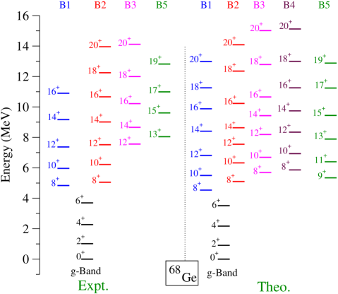
Figure 1: (Color online) Comparison of the calculated energies with available experimental data for ⁶⁸Ge. Data is taken from ref. [39].

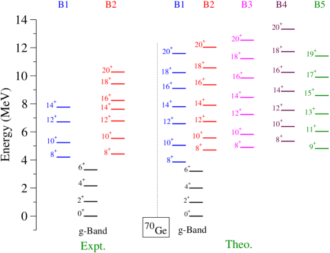
Figure 2: (Color online) Comparison of the calculated energies with available experimental data for ⁷⁰Ge. Data is taken from ref. [15, 45].

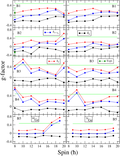
Figure 3: (Color online) ^68,70Ge g-factor with attenuated magnetic charges. The green line shows $Z/A$.

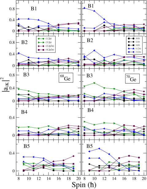
Figure 4: (Color online) Probability of various projected K-configurations in the wavefunctions of the excited bands in ^68,70Ge. For clarity, only the lowest projected K-configurations in the wavefunctions of bands are shown and in the numerical calculations, projection has been performed from more than forty intrinsic states.

The second s-band in ⁷⁰Ge, labelled as band B2 in Fig. 2, was recently populated [15] and it has been shown using cranked shell model (CSM) approach that this band could not be attributed to the alignment of two-protons as crossing of this structure with the ground-state band is expected around $\hbar\omega=0.9$MeV. In the experimental data, both band B1 and B2 cross the ground-state band at $\hbar\omega=0.5$ MeV. In CSM analysis, neutron crossing occurs around this frequency and, therefore, both the bands are expected to have neutron character. TPSM results indicate [15] that band B2 is the $\gamma$-band based on two-neutron aligned structure and crosses the ground-state band at the same rotational frequency as that of the parent band B1.

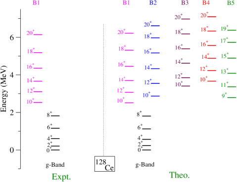
Figure 5: (Color online) Comparison of the calculated energies with available experimental data for ¹²⁸Ce. Data is taken from ref. [46].

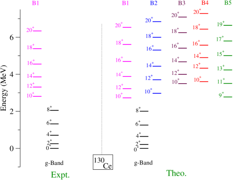
Figure 6: (Color online) Comparison of the calculated energies with available experimental data for ¹³⁰Ce. Data is taken from ref. [47].

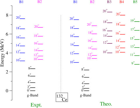
Figure 7: (Color online) Comparison of the calculated energies with available experimental data for ¹³²Ce. Data is taken from ref. [48].

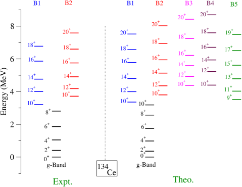
Figure 8: (Color online) Comparison of the calculated energies with available experimental data for ¹³⁴Ce. Data is taken from ref. [49].

In order to quantify the intrinsic neutron and proton content, g-factors have been evaluated for the excited band structures. As the single particle neutron and proton gyromagnetic ratios have opposite signs with $g_{n}=-1.91$ and $g_{p}=2.79$, the measurement of g-factors provides information on the proton/neutron structure of a given state. The calculated g-factors, using the TPSM wavefunction and the expression, Eq. 7, for ⁶⁸Ge and ⁷⁰Ge are displayed in Fig. 3 for all the excited band structures of Figs. 1 and 2. Apart from the total g-factor, individual neutron and proton g-factor, labelled as $g_{n}$ and $g_{p}$, and the rigid value of Z/A are also depicted in these figures. First of all, it is evident from the figure that aside from some minor variation, the overall behaviour of the g-factors with spin for the two nuclei is very similar. For band B1 in both nuclei, the total g-factor for spin values up to I=12 is negative, indicating that this band is dominated by neutron configuration. This is evident from the wavefunction decomposition of the band structures of two nuclei plotted in Fig. 4. Band B1 is noted to be dominated by $(1,2n)$, which is a two-neutron aligned configuration with K=1 up to I=12. For I=14 and above, it is observed that $(2,2p2n)$ and $(4,2p2n)$ configurations, which are four-quasiparticle states with K=2 and 4, respectively, dominate. Since one-particle proton g-factor is much larger than the corresponding neutron g-factor, the total g-factor is positive for the two-proton plus two-neutron state above I=14 in Fig. 4.

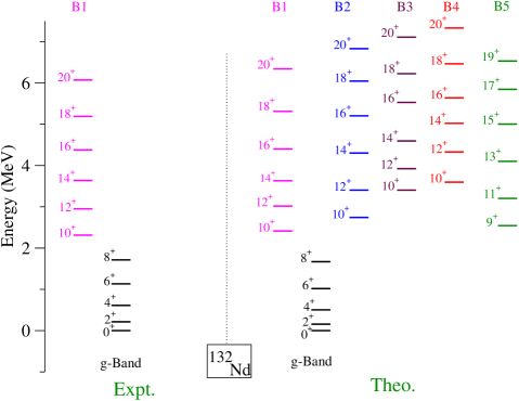
Figure 9: (Color online) Comparison of the calculated energies with available experimental data for ¹³²Nd. Data is taken from ref. [50].

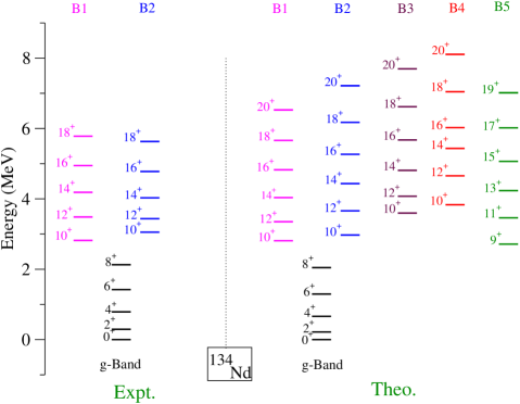
Figure 10: (Color online) Comparison of the calculated energies with available experimental data for ¹³⁴Nd. Data is taken from ref. [51].

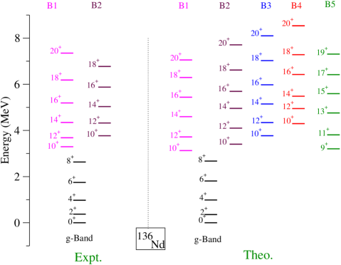
Figure 11: (Color online) Comparison of the calculated energies with available experimental data for ¹³⁶Nd. Data is taken from ref. [52].

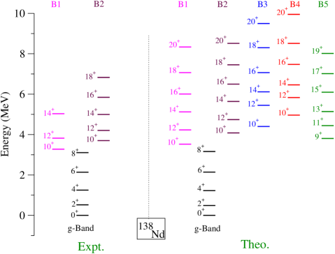
Figure 12: (Color online) Comparison of the calculated energies with available experimental data for ¹³⁸Nd. Data is taken from ref. [53].

It is interesting to note in Fig. 3 that band B2 has a similar g-factor values as that of the band B1. The reason for this similarity can be easily inferred from the wavefunction decomposition of band B2 plotted in Fig. 4. This band is dominated by $(3,2n)$ configuration, which is the $\gamma$-band based on the two-neutron aligned configuration, $(1,2n)$. Since the two configurations have similar intrinsic structure, the g-factors of the two bands are expected to be similar. This naturally explains why the observed gyromagnetic ratios of the I=8 states of bands B1 and B2 in ⁶⁸Ge have similar g-factors. In the earlier work, higher multipole interaction in the particle-rotor model picture was invoked [40] to explain this apparent anomally. It is not clear, at this stage, how this can be related to the results obtained in the present work. The experimental g-factors for I=8 states of the bands B1 and B2 are also plotted in Fig. 3 for ⁶⁸Ge. For band B1, the measured value is about g=0.1 [40], which indicates that the state has neutron character and the TPSM calculations predict neutron character for the state with g = -0.26. For band B2, both measured and the calculated g-factors are negative and have similar values.

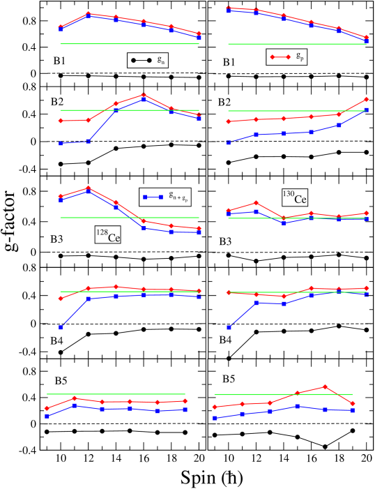
Figure 13: (Color online) ^128,130Ce g-factor with attenuated magnetic charges. The green line shows $Z/A$.

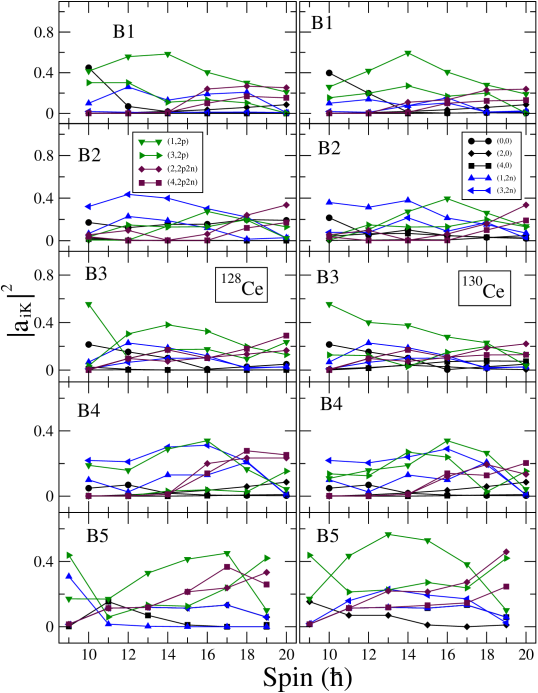
Figure 14: (Color online) Probability of various projected K-configurations in the wavefunctions of the observed bands for ^128,130Ce. For clarity, only the lowest projected K-configurations in the wavefunctions of bands are shown and in the numerical calculations, projection has been performed from more than forty intrinsic states.

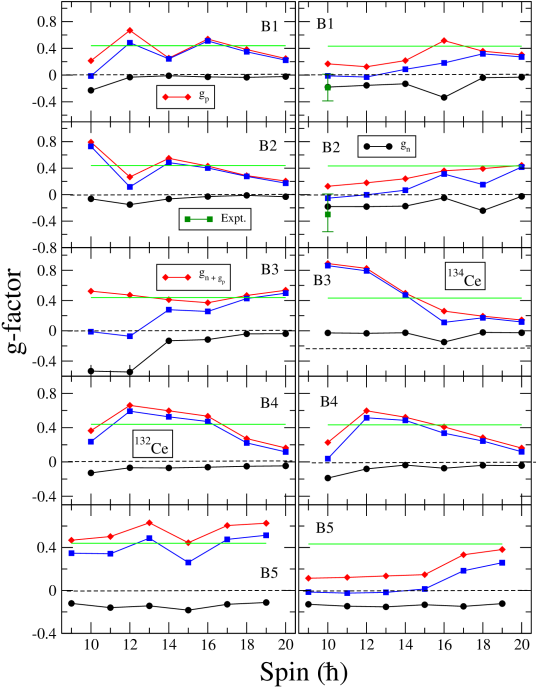
Figure 15: (Color online) ^132,134Ce g-factor with attenuated magnetic charges. The green line shows $Z/A$.

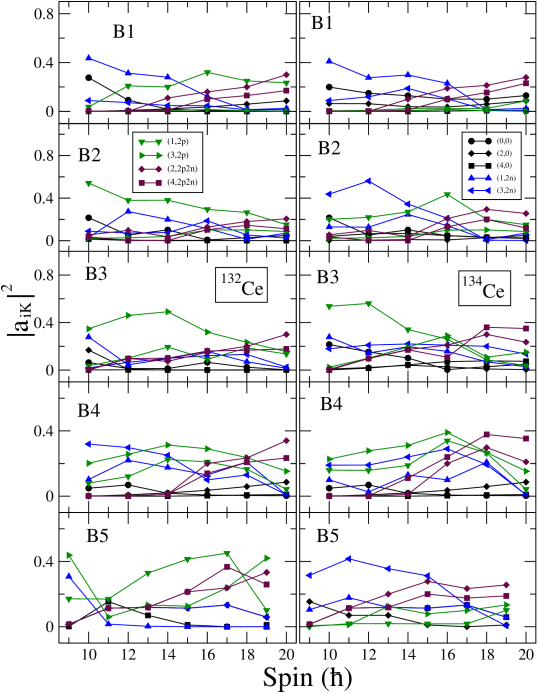
Figure 16: (Color online) Probability of various projected K-configurations in the wavefunctions of the observed bands for ^132,134Ce. For clarity, only the lowest projected K-configurations in the wavefunctions of bands are shown and in the numerical calculations, projection has been performed from more than forty intrinsic states.

The total g-factors of Bands B3 and B4 in Fig. 3 for both nuclei are positive, indicating that proton component is dominant for these band structures. This is evident from the wavefunction plot of Fig. 4 with band B3 dominated by $(1,2p)$ component, which is a proton aligned configuration with K=1. The g-factors of band B4 are similar as that of band B3 and from the wavefunction analysis, it is noted that band B4 is dominated by $(3,2p)$, which is a $\gamma$-band built on $(1,2p)$ aligned state. Band B5 for both the nuclei has a larger component of $(3,2n)$ configuration, but there are also significant other contributions. This mixing of various components leads to almost vanishing of the total g-factor for this particular band structure, except for high spin states from I=17 to 19 in ⁶⁸Ge.

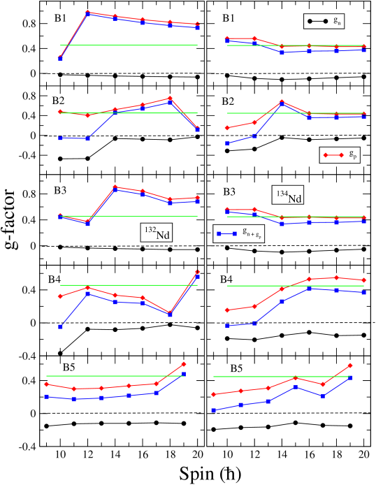
Figure 17: (Color online) ^132,134Nd g-factor with attenuated magnetic charges. The green line shows $Z/A$.

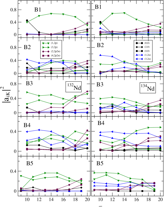
Figure 18: (Color online) Probability of various projected K-configurations in the wavefunctions of the observed bands for ^132,134Nd. For clarity, only the lowest projected K-configurations in the wavefunctions of bands are shown and in the numerical calculations, projection has been performed from more than forty intrinsic states.

For Ce and Nd isotopes around A$\sim$130, forking of the ground-state into s-bands has been observed [41, 42] and in the present work we have evaluated g-factors for these band structures. It has been demonstrated in our earlier work [11] that in some of these nuclei, $\gamma$-bands built on two-quasiparticle structure becomes favoured in energy as for Ge-isotopes studied above. This lowering of the $\gamma$-band was proposed to be the reason for observation of the g-factors of the band heads of the two s-bands with the same sign [11]. However, g-factors were not evaluated in our previous work and in the following g-factors shall be presented for lowest s-band structures as has been done for Ge isotopes.

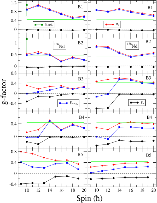
Figure 19: (Color online) ^136,138Nd g-factor with attenuated magnetic charges. The green line shows $Z/A$.

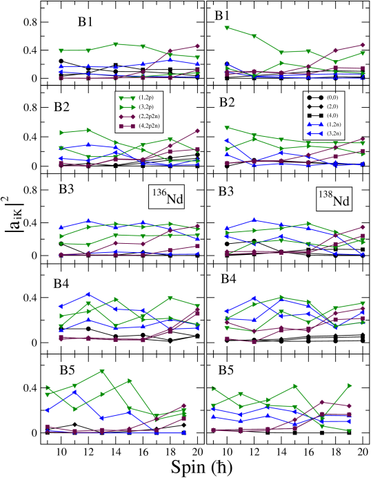
Figure 20: (Color online) Probability of various projected K-configurations in the wavefunctions of the observed bands for ^136,138Nd. For clarity, only the lowest projected K-configurations in the wavefunctions of bands are shown and in the numerical calculations, projection has been performed from more than forty intrinsic states.

For completeness, we shall first discuss the comparison between the observed and the TPSM calculated band structures of these nuclei before presenting the g-factors. The band structures for ¹²⁸Ce, ¹³⁰Ce, ¹³²Ce and ¹³⁴Ce are displayed in Figs. 5, 6, 7 and 8. For all studied isotopes of Ce, multiple s-band structures are predicted and only for ¹³²Ce and ¹³⁴Ce, two s-band structures are observed and it is noted from these figures that observed energies are reproduced reasonably well by TPSM calculations. Also, TPSM calculated band structures for ¹³²Nd, ¹³⁴Nd, ¹³⁶Nd and ¹³⁸Nd are presented in Figs. 9, 10, 11 and 12. The band structures show similiar behaviour as that of Ce-isotopes and are reproduced quite well by the calculations.

The calculated TPSM energies for all the isotopes studied in the present work are also displayed as numbers in Table 2 so that other quantities of interest, for instance, the alignments and moments of inertia, can be calculated and compared with other model predictions.

TPSM calculated g-factors for the ¹²⁸Ce and ¹³²Ce are plotted in Fig. 13 along with the rigid value of Z/A. The behaviour of the g-factors for ¹²⁸Ce and ¹³⁰Ce is quite similar and can be easily understood from the corresponding wavefunction plot of Fig.  14. It is noted from this figure that band B1 is dominated by two-proton aligned configuration, $(1,2p)$ and the corresponding total g-factor in Fig. 13 is positive. On the other hand, band B2 has dominant component of $(1,2n)$, which is a two-neutron aligned configuration, and the corresponding g-factor is negative in Fig. 13. As already explained earlier, the one-particle g-factor for proton is quite large as compared to the corresponding neutron g-factor, a small proton component in the wavefuction makes the total g-factor skewed towards positive values. Therefore, the total g-factor for band B2 in Fig. 13, close to zero for spin values of I=10 and 12, indicates that this band, for these spin values, is dominated by neutron configuration. For high-spin states, band B2 is dominated by four-quasiparticle configurations and the total g-factor tends to approach large positive values. Band B3 in Fig. 14 is dominated by two-proton aligned states of $(1,2p)$ and $(3,2p)$ for ¹²⁸Ce and ¹³⁰Ce, respectively and consequently g-factors in Fig. 13 have large positive values. For bands B4 and B5, the wavefunctions in Fig. 14 are highly mixed and the g-factors tend to be slightly positive. However, for high-spin states, the wavefunction is dominated by four-quasiparticle configurations and the g-factors acquire large positive values.

TPSM calculated g-factors for ¹³²Ce and ¹³⁴Ce are displayed in Fig. 15 along with the rigid value of Z/A and the corresponding wavefunctions are displayed in Fig. 16. For band B1, the total g-factors in Fig. 15 are negative for the low-spin states as the wavefunction for this band is dominated by the neutron aligned configuration, $(1,2n)$. There is a major difference in the wavefunctions of the band B2 for two nuclei. In ¹³²Ce, band B2 is dominated by the aligned two-proton state, $(1,2p)$, whereas in ¹³⁴Ce this band is dominated by $(3,2n)$, which is the $\gamma$-band based on two-neutron aligned configuration. This results into positive and negative g-factors of band B2 in two nuclei for low-spin states in Fig. 15. Therefore, for ¹³²Ce the two observed s-bands are expected to have opposite g-factors and for ¹³⁴Ce, both the s-bands should have negative g-factors as the two bands have same intrinsic neutron configuration. As a matter of the fact, this is confirmed by the experimental work performed in [44] and the observed values are plotted in Fig. 15. Both the measured g-factors of the I=10 states of the two s-bands being negative was an unresolved issue. It was explained in our earlier publication and now backed up with numbers, that band B2 in ¹³⁴Ce has the same intrinsic configuration as that of band B1. The only difference is that band B2 is the $\gamma$-band based on band B1.

In Fig. 16, band B3 in ¹³²Ce and ¹³⁴Ce are dominated by $(3,2p)$ and $(1,2p)$ configurations, respectively. Since both these are proton configurations, the g-factors for this band are positive in Fig. 15. The wavefunctions for bands B4 and B5 in Fig. 16 are highly mixed for two nuclei and the corresponding g-factors also reflect this mixing.

The g-factors for ¹³²Nd and ¹³⁴Nd are shown in Fig. 17 along with the rigid value of Z/A and the corresponding wavefunctions are depicted in Fig. 18. The g-factors for band B1 in both the nuclei are positive as the wavefunction has the dominant proton aligned configuration, $(1,2p)$. Band B2, on the other hand, is dominated by the neutron aligned configuration, $(1,2n)$ for low-spin values and, therefore, corresponding g-factors are negative for these spin values. For high-spin states, four-quasiparticle configurations become important and consequently g-factors tend to acquire positive values with increasing spin. Band B3 for both the nuclei is mostly composed of $(3,2p)$ and, therefore, the g-factors are positive for this band structure. As is evident from Fig. 17 that bands B4 and B5 are highly mixed with the consequence that g-factors are between neutron and proton maximal values.

The results for ¹³⁶Nd and ¹³⁸Nd are plotted in Figs. 19 and 20 along with the rigid value of Z/A. It is interesting to note from Fig.19 that g-factors for the lowest two bands, B1 and B2, for both the nuclei are positive. The reason for this is evident from the wavefunction decomposition in Fig. 20 with the two bands dominated by $(1,2p)$ and $(3,2p)$, respectively. This result is opposite to that obtained for ¹³⁴Ce, where lowest two bands have neutron configurations dominant. The experimental values available for the I=10 state in bands B1 and B2 for ¹³⁶Nd are also positive and in good agreement with the calculated values. Bands B3 and B4 in Fig. 19 have negative g-factors for low-spin states as these bands have dominant two-neutron aligned configurations. Band B5 is highly mixed with the g-factors in Fig. 19 depicting intermediate behaviour for some spin values. For completeness, the attenuated g-factors for the ground-state bands of all the nuclei studied in the present work are provided in Table 3.

Table 2: TPSM calculated energies for g-band and excited band structures of ^68,70Ge, ^{128,130,132,134}Ce, and ^{132,134,136,138}Nd isotopes.

68Ge
I($\hbar$)	g-band	I($\hbar$)	B1	B2	B3	B4	I($\hbar$)	B5
0	0.0	8	4.535	5.098	5.691	5.865	9	5.343
2	0.905	10	5.497	6.323	6.689	6.932	11	6.397
4	2.170	12	6.811	7.549	8.189	8.342	13	7.887
6	3.511	14	8.404	8.634	9.428	9.743	15	9.442
		16	9.881	10.231	10.655	11.254	17	11.239
		18	11.254	12.354	12.788	12.993	19	12.880
		20	12.986	14.086	15.016	15.121
70Ge
0	0.0	8	3.854	4.708	4.898	5.332	9	4.817
2	0.980	10	5.046	5.571	5.823	6.383	11	6.034
4	1.996	12	6.583	6.738	7.238	7.538	13	7.284
6	3.199	14	7.796	7.905	8.455	8.895	15	8.592
		16	9.097	9.360	9.841	10.241	17	9.897
		18	10.221	10.558	11.221	11.721	19	11.408
		20	11.587	12.034	12.532	13.322
128Ce
0	0.0	10	2.515	2.871	3.407	3.667	9	2.791
2	0.234	12	3.072	3.547	3.851	4.229	11	3.367
4	0.566	14	3.697	4.330	4.621	4.883	13	4.086
6	1.122	16	4.457	5.169	5.389	5.566	15	4.893
8	1.806	18	5.316	5.975	6.182	6.334	17	5.735
		20	6.218	6.615	6.977	7.097	19	6.378
130Ce
0	0.0	10	2.728	2.975	3.500	3.606	9	2.775
2	0.213	12	3.224	3.707	3.999	4.329	11	3.507
4	0.646	14	3.882	4.436	4.675	4.901	13	4.236
6	1.258	16	4.693	5.308	5.410	5.573	15	5.008
8	2.008	18	5.611	5.997	6.249	6.438	17	5.797
		20	6.533	6.842	7.089	7.284	19	6.642
132Ce
0	0.0	10	2.988	3.408	4.002	4.067	9	2.788
2	0.250	12	3.915	3.733	5.006	4.531	11	3.715
4	0.740	14	4.774	4.417	5.754	5.178	13	4.574
6	1.416	16	5.718	5.191	6.331	5.966	15	5.418
8	2.195	18	6.582	6.019	7.193	6.934	17	6.383
		20	7.521	6.877	8.323	7.997	19	7.321
134Ce
0	0.0	10	3.361	3.801	4.378	4.398	9	3.517
2	0.360	12	3.998	4.357	4.929	5.227	11	4.029
4	0.983	14	4.801	5.130	5.588	5.937	13	4.788
6	1.749	16	5.780	5.943	6.215	6.710	15	5.615
8	2.567	18	6.566	6.945	7.250	7.595	17	6.505
		20	7.521	8.023	8.428	8.696	19	7.502
132Nd
0	0.0	10	2.414	2.743	3.404	3.597	9	2.543
2	0.156	12	3.017	3.404	3.923	4.329	11	3.204
4	0.504	14	3.630	4.302	4.594	5.022	13	4.102
6	1.018	16	4.400	5.204	5.529	5.641	15	5.004
8	1.670	18	5.312	6.046	6.226	6.465	17	5.846
		20	6.341	6.831	7.111	7.331	19	6.531
134Nd
0	0.0	10	2.809	2.971	3.595	3.833	9	2.714
2	0.216	12	3.349	3.660	4.073	4.655	11	3.461
4	0.662	14	4.035	4.433	4.809	5.433	13	4.233
6	1.294	16	4.827	5.265	5.673	6.024	15	5.065
8	2.047	18	5.661	6.172	6.618	7.044	17	6.017
		20	6.526	7.214	7.694	8.108	19	7.014
136Nd
0	0.0	10	3.128	3.403	3.770	4.295	9	3.203
2	0.356	12	3.719	4.097	4.341	4.946	11	3.809
4	0.987	14	4.596	4.956	5.146	5.482	13	4.756
6	1.810	16	5.439	5.693	5.977	6.423	15	5.593
8	2.673	18	6.293	6.617	7.025	7.282	17	6.417
		20	7.053	7.707	8.100	8.533	19	7.307
138Nd
0	0.0	10	3.522	4.081	4.401	4.962	9	3.808
2	0.489	12	4.230	4.742	5.447	5.831	11	4.442
4	1.225	14	5.123	5.639	6.113	6.459	13	5.139
6	2.140	16	6.006	6.495	7.066	7.472	15	6.095
8	3.162	18	7.065	7.453	8.298	8.512	17	7.015
		20	8.337	8.514	9.497	9.951	19	8.014

Table 3: Calculated and measured g-factors for ground-state bands of ^68,70Ge, ^{128,130,132,134}Ce, and ^{132,134,136,138}Nd isotopes.

I($\hbar$)	68Ge	70Ge	128Ce	130Ce	132Ce	134Ce	132Nd	134Nd	136Nd	138Nd
2	0.02	0.04	0.03	0.02	0.06	0.04	0.02	0.05	0.04	0.07
Expt.								0.6${}^{+4}_{-4}$
4	-0.06	-0.07	0.05	0.08	0.03	0.05	0.03	0.05	0.06	0.01
6	-0.18	-0.20	0.02	0.08	-0.10	-0.08	0.06	0.09	0.03	0.03
8			0.15	0.23	-0.17	-0.08	0.12	0.17	0.06	0.27

4 Summary and Conclusions

The purpose of the present work has been to perform a systematic analysis of the g-factors of the excited band structures observed in selected isotopes of Ge, Ce and Nd. These selected isotopes are predicted to depict forking of the ground-state into several s-bands. In most of the nuclei, ground-state band is crossed by quasiparticle aligned band, which in most of the cases has a two-neutron character. However, for nuclei studied in the present work, gound-state band is crossed by several band structures simultaneously. For these nuclei, the Fermi surfaces of neutrons and protons are similar and, therefore, both neutron and proton aligned bands are expected to cross the ground-state band simultaneously. In some of these nuclei, the excited bands depict this expected structure. However, ⁶⁸Ge and ¹³⁴Ce display two s-bands with the same neutron structure and for ¹³⁶Nd the bands have the same proton character. The g-factors calculated using the TPSM wavefunctions reproduce the neutron character for ⁶⁸Ge and ¹³⁴Ce, and proton structure for ¹³⁶Nd.

It is evident from the TPSM analysis that each triaxial intrinsic state has a $\gamma$- band built on it. The triaxial ground- or vacuum-state is a superposition of K=0, 2, 4,… configurations and the angular-momentum projection of the K=0 state corresponds to the ground-state band. The projection of K=2 and 4 lead to the $\gamma$- and $\gamma\gamma$-bands. In a similar manner, the two-quasiparticle aligned state is a superposition of K=1,3,5….. The angular-momentum projection of K=1 state leads to the normal s-band and the projection with K=3 corresponds to the $\gamma$-band built on the two-quasiparticle aligned state. In some nuclei, this $\gamma$-band becomes favoured as compared to other configurations and crosses the ground-state band. In ⁶⁸Ge and ¹³⁴Ce, the lowest two aligned bands that cross the ground-state band are the two-neutron aligned band and the $\gamma$-band built on this state. For ¹³⁶Nd the lowest two bands have proton character. Since these bands have the same intrinsic configuration, g-factors of the two band structures are also expected to be similar. Therefore, TPSM analysis provides a natural explanation for the observation of neutron g-factors for the bandheads of two lowest aligned band structures in ⁶⁸Ge and ¹³⁴Ce and proton for ¹³⁶Nd.

Further, it has been predicted that observed two s-bands in ⁷⁰Ge should also have negative g-factors. For the case of ¹³⁸Nd, the lowest two s-bands are predicted to have positive g-factors. It would be quite interesting to perform the g-factor measurements of these nuclei to verify the predictions of the present model analysis. It would be also interesting to explore other nuclei having $\gamma$-bands based on excited quasiparticle configurations.

References

- [1] A. Bohr and B. R. Mottelson, Nuclear Structure, Vol. II (Benjamin Inc., New York, 1975).
- [2] M. G. Mayer and J. H. D. Jensen, Elementry Theory of Nuclear Shell Structure (John Wiley Sons, New York, 1955).
- [3] S. Frauendorf, Rev. Mod. Phys. 73 (2001) 463.
- [4] O. Kenn, K.-H. Speidel, R. Ernst, J. Gerber, P. Maier-Komor and F. Nowacki, Phys. Rev. C63 (2001) 064306, and the references cited therein.
- [5] F. Brandolini, M. De Poli, P. Pavan, R.V. Ribas, D. Bazzacco and C.R. Rossi-Alvarez, Eur. Phys. J. A6 (1999) 149.
- [6] I. Alfter, E. Bodenstedt, W. Knichel and J. Schüth, Z. Phys. A355 (1996) 277.
- [7] D. R. Jensen, G. B. Hagemann, I. Hamamoto, S. W. Ødegård, B. Herskind, G. Sletten, J. N. Wilson, K. Spohr, H. Hübel, P. Bringel Phys. Rev. Lett. 89 (2002) 142503.
- [8] R. M. Clark, S. J. Asztalos, G. Baldsiefen, J. A. Becker, L. Bernstein, M. A. Deleplanque, R. M. Diamond, P. Fallon, I. M. Hibbert, H. Hübel Phys. Rev. Lett. 78 (1997) 1868.
- [9] H. Iwasaki, A. Lemasson, C. Morse, A. Dewald, T. Braunroth, V. M. Bader, T. Baugher, D. Bazin, J. S. Berryman, C. M. Campbell Phys. Rev. Lett. 112 (2014) 142502.
- [10] J.A. Sheikh, G.H. Bhat, Y. Sun, G.B. Vakil, R. Palit, Phys. Rev. C 77 (2008) 034313.
- [11] J.A. Sheikh, G.H. Bhat, R. Palit, Z. Naik, Y. Sun, Nucl. Phys. A 824 (2009) 58.
- [12] S. Frauendorf, J. Meng, Nucl. Phys. A 617 (1997) 131.
- [13] V. I. Dimitrov, S. Frauendorf, F. Dönau, Phys. Rev. Lett. 84 (2000) 5732.
- [14] J.A. Sheikh and K. Hara, Phys. Rev. Lett. 82 (1999) 3968.
- [15] M. Kumar Raju, P. V. Madhusudhana Rao, S. Muralithar, R. P. Singh, G. H. Bhat, J. A. Sheikh, S. K. Tandel, P. Sugathan, T. Seshi Reddy, B. V. Thirumala Rao, and R. K. Bhowmik, Phys. Rev C 93 (2016) 034317.
- [16] M. Sugawara, Y. Toh, M. Oshima, M. Koizumi, A. Kimura, A. Osa, Y. Hatsukawa, H. Kusakari, J. Goto, M. Honma, M. Hasegawa, and K. Kaneko, Phys. Rev. C 81 (2010) 024309.
- [17] B. Mukherjee, S. Muralithar, G. Mukherjee, R. P. Singh, R. Kumar, J. J. Das, P. Sugathan, N. Madhavan, P. V. M. Rao, A. K. Sinha, A. K. Pande, L. Chaturvedi, S. C. Pancholi, and R. K. Bhowmik, Acta Phys. Hung. N.S.11 (2000) 189.
- [18] C. Morand, M. Agard, J. F. Bruandet, A. Giorni, J. P. Longequeue, and Tsan Ung Chan, Phys. Rev. C 13 (1976) 2182.
- [19] R. L. Robinson, H. J. Kim, R. O. Sayer, Jr. J. C. Wells, R. M. Ronningen and J. H. Hamilton, Phys. Rev. C 16 (1977) 6.
- [20] R. Bengtsson, and S. Frauendorf Nucl. Phys. A 327, 139 (1979).
- [21] P. Ring and P. Schuck, The Nuclear Many Body Problem (Springer-Verlag, New York), (1980).
- [22] K. Hara and S. Iwasaki, Nucl. Phys. A 332 (1979) 61.
- [23] K. Hara and S. Iwasaki, Nucl. Phys. A 348 (1980) 200.
- [24] S. N. T. Majola, D. J. Hartley, L. L. Riedinger, J. F. Sharpey-Schafer, J. M. Allmond, C. Beausang, M. P. Carpenter, C. J. Chiara, N. Cooper, D. Curien, B. J. P. Gall, P. E. Garrett, R. V. F. Janssens, F. G. Kondev, W. D. Kulp, T. Lauritsen, E. A. McCutchan, D. Miller, J. Piot, N. Redon, M. A. Riley, J. Simpson, I. Stefanescu, V. Werner, X. Wang, J. L. Wood, C.-H. Yu, and S. Zhu, Phys. Rev. C 91 (2015) 034330.
- [25] S. Jehangir, G.H. Bhat, J.A. Sheikh, S. Frauendorf, S.N.T. Majola, P.A. Ganai and J.F. Sharpey-Schafer (to be published).
- [26] K. Hara and Y. Sun, Int. J. Mod. Phys. E 4 (1995) 637.
- [27] S. G. Nilsson, C. F. Tsang, A. Sobiczewski, Z. Szymanski, S. Wycech, C. Gustafson, I. Lamm, P. Moller, and B. Nilsson, Nucl. Phys. A 131 (1969) 1.
- [28] J.A. Sheikh, G.H. Bhat, Y.-X. Liu, F.-Q. Chen, and Y. Sun, Phys. Rev. C 84 (2011) 054314.
- [29] C. Zhang, G. H. Bhat, W. Nazarewicz, J. A. Sheikh, and Y. Shi, Phys. Rev. C 92 (2015) 034307.
- [30] P. Boutachkov, A. Aprahamian, Y. Sun, J.A. Sheikh, S. Frauendorf, Eur. Phys. J. A 15 (2002) 455.
- [31] G. H. Bhat, J. A. Sheikh, Y. Sun, and U. Garg, Phys. Rev. C 86 (2012) 047307.
- [32] J.A. Sheikh, Y. Sun, R. Palit, Phys. Lett. B 507 (2001) 115.
- [33] F.-Q. Chen, Y. Sun, P. M. Walker, G. D. Dracoulis, Y. R. Shimizu, and J. A. Sheikh, J. Phys. G 40 (2013) 015101.
- [34] Y. Sun, G.-L. Long, F. Al-Khudair, and J. A. Sheikh, Phys. Rev. C 77, 044307 (2008).
- [35] Y. Sun, J.A. Sheikh, and G.-L. Long, Phys. Lett. B 533 (2002) 253.
- [36] S. Raman, C. H. Malarkey, W. T. Milner, C. W. Nestor, Jr., and P. H. Stelson, Atom. Data Nucl. Data Tables 36 (1987) 1.
- [37] P. Möller and J.R. Nix, At. Data Nucl. Data Tables 59 (1995) 185.
- [38] E. A. Stefanova, I. Stefanescu, G. de Angelis, D. Curien, J. Eberth, E. Farnea, A. Gadea, G. Gersch, A. Jungclaus, K. P. Lieb, T. Martinez, R. Schwengner, T. Steinhardt, O. Thelen, D. Weisshaar, and R. Wyss, Phys. Rev. C 67, 054319 (2003).
- [39] D. Ward, C. E. Svensson, I. Ragnarsson, C. Baktash, M. A. Bentley, J. A. Cameron, M. P. Carpenter, R. M. Clark, M. Cromaz, M. A. Deleplanque, M. Devlin, R. M. Diamond, P. Fallon, S. Flibotte, A. Galindo-Uribarri, D. S. Haslip, R. V. F. Janssens, T. Lampman, G. J. Lane, I. Y. Lee, F. Lerma, A. O. Macchiavelli, S. D. Paul, D. Radford, D. Rudolph, D. G. Sarantites, B. Schaly, D. Seweryniak, F. S. Stephens, O. Thelen, K. Vetter, J. C. Waddington, J. N. Wilson, and C.-H. Yu, Phys. Rev. C 63 (2000) 014301.
- [40] M. E. Barclay, L. Cleemann, A. V. Ramayya, J. H. Hamilton, C. F. Maguiret, W. C. Mat, R. Soundranayagamt, K. Zhaotb, A. Balandat, J. D. ColeSd, R. B. Pierceyg, A. Faessler, and S. Kuyucak, J. Phys. G 12 (1986) 295.
- [41] R. Wyss, A. Granderath, R. Bengtsson, P. Von Brentano, A. Dewald, A. Gelberg, A. Gizon, J. Gizon, S. Harrisopulos, A. Jhonson, W. Lieberz, W. Nazarwicz, J. Nyberg, and K. Schiffer, Nucl. Phys. A 505 (1989) 337.
- [42] R. Wyss, J. Nyberg, A. Johnson, R. Bengtsson and W. Nazarewicz, Phys. Lett. B 215 (1988) 211.
- [43] W. Satula and R. Wyss, Physica Scripta T 56 (1995) 159.
- [44] A. Zemel, C. Broude, E. Dafni, A. Gelberg, M. B. Goldberg, J. Gerber, G. J. Kumbartzki, and K. -H. Speidel, Nucl. Phys. A 383 (1982) 165.
- [45] J. K. Tuli, Nucl. Data Sheets 103 (2004) 389.
- [46] E. S. Paul, P. Bednarczyk, A. J. Boston, C. J. Chiara, C. Foin, D. B. Fossan, A. Gizon, J. Gizon, D. G. Jenkins, N. Kelsall, N. Kintz, P. J. Nolan, B. M. Nyako, C. M. Parry, J. A. Sampson, A. T. Semple, K. Starosta, J. Timar, A. N. Wilson, and L. Zolnai, Nucl. Phys. A 676 (2000) 32.
- [47] B. Singh, Nucl. Data Sheets 93 (2001) 33.
- [48] E. S. Paul, P. T. W. Choy, C. Andreoiu, A. J. Boston, A. O. Evans, C. Fox, S. Gros, P. J. Nolan, G. Rainovski, J. A. Sampson, H. C. Scraggs, A. Walker, D. E. Appelbe, D. T. Joss, J. Simpson, J. Gizon, A. Astier, N. Buforn, A. Prvost, N. Redon, O. Stzowski, B. M. Nyak, D. Sohler, J. Timr, L. Zolnai, D. Bazzacco, S. Lunardi, C. M. Petrache, P. Bednarczyk, D. Curien, N. Kintz, and I. Ragnarsson, Phys Rev. C 71 (2005) 054309.
- [49] A. A. Sonzogni, Nucl. Data Sheets 103 (2004) 1.
- [50] Yu. Khazov et al., Nucl. Data Sheets 104 (2005) 497.
- [51] C. M. Petrache, D. Bazzacco, S. Lunardi, C. R. Alvarez, R. Venturelli, R. Burch, P. Pavan, G. Maron, D. R. Napoli, L. H. Zhu, and R. Wyss, Phys. lett. B 387 (1996) 31.
- [52] O. Zeidan, D. J. Hartley, L. L. Reidinger, W. Reviol, W. D. Weintraub, Y. Sun, and Jing-ye Zhang, Phys. Rev. C 66 (2002) 044311.
- [53] E. Mergel, C. M. Petrache, G. Lo Bianco, H. Hubel, J. Domscheit, N. Nenoff, A. Neuver, A. Gorgen, F. Becker, E. Bouchez, M. Houry, W. Korten, A. Bracco, N. Blasi, F. Camera, S. Leoni, F. Hannachi, M. Rejmund, P. Reiter, P. G. Thirolf, A. Astier, N. Redon, and O. Stezowski, Eur. Phys. J. A 15 (2002) 417.