Studying the ICM in clusters of galaxies via surface brightness fluctuations of the cosmic X-ray background

Abstract

We study the surface brightness fluctuations of the cosmic X-ray background (CXB) using Chandra data of XBOOTES. After masking out resolved sources we compute the power spectrum of fluctuations of the unresolved CXB for angular scales from $\approx 2\arcsec$ to $\approx 3^{\circ}$. The non-trivial large-scale structure (LSS) signal dominates over the shot noise of unresolved point sources at all scales above $\sim 1\arcmin$ and is produced mainly by the intracluster medium (ICM) of unresolved clusters and groups of galaxies, as shown in our previous publication.

The shot-noise-subtracted power spectrum of CXB fluctuations has a power-law shape with the slope of $\Gamma=0.96\pm 0.06$. Its energy spectrum is well described by the redshifted emission spectrum of optically-thin plasma with the best-fit temperature of $T\approx 1.3$ keV and the best-fit redshift of $z\approx 0.40$. They are in good agreement with theoretical expectations based on the X-ray luminosity function and scaling relations of clusters. From these values we estimate the typical mass and luminosity of the objects responsible for CXB fluctuations, $M_{500}\sim 10^{13.6}\,\mathrm{M_{\sun}}\,h^{-1}$ and $L_{0.5-2.0\,{\rm keV}}\sim 10^{42.5}\,\mathrm{erg\,s^{-1}}$. On the other hand, the flux-weighted mean temperature and redshift of resolved clusters are $T\approx 2.4$ keV and $z\approx 0.23$, confirming that fluctuations of unresolved CXB are caused by cooler (i.e. less massive) and more distant clusters, as expected. We show that the power spectrum shape is sensitive to the ICM structure all the way to the outskirts, out to $\sim{\rm few}\times R_{500}$. We also look for possible contribution of the warm-hot intergalactic medium (WHIM) to the observed CXB fluctuations.

Our results underline the significant diagnostics potential of the CXB fluctuation analysis in studying the ICM structure in clusters.

1 Introduction

Since the discovery of the cosmic X-ray background (CXB) more than half a century ago (Giacconi et al., 1962), analyzing its surface brightness fluctuations via angular correlation studies has been a powerful tool in understanding the origin of the CXB (e.g. Scheuer, 1974; Hamilton & Helfand, 1987; Shafer & Fabian, 1983; Barcons & Fabian, 1988; Soltan & Hasinger, 1994; Vikhlinin & Forman, 1995; Miyaji & Griffiths, 2002). Such CXB fluctuation analyses have suggested very early on that the CXB is dominated by extragalactic discrete sources, with Active Galactic Nuclei (AGN) leading the way, and that their redshift distribution is similar to optical QSOs but with somewhat higher clustering strength. These results were confirmed during the last $\sim$two decades with the resolved X-ray sources through their source counts with very deep pencil beam surveys (e.g. Brandt & Hasinger, 2005; Alexander et al., 2013; Brandt & Alexander, 2015; Lehmer et al., 2012; Luo et al., 2017) and large-scale structure (LSS) studies with much wider but shallower surveys (see reviews of Cappelluti, Allevato & Finoguenov, 2012; Krumpe, Miyaji & Coil, 2014).

The CXB is an ideal laboratory for studying growth and co-evolution of supermassive black holes (SMBH) with their dark matter halo (DMH) up to high redshift ($z\sim 5$, e.g. Hasinger, Miyaji & Schmidt, 2005; Gilli, Comastri & Hasinger, 2007; Aird et al., 2010; Ueda et al., 2014; Miyaji et al., 2015), which is a keystone in understanding galaxy evolution over cosmic time (e.g. Hopkins et al., 2006; Hickox et al., 2009; Alexander & Hickox, 2012; Heckman & Best, 2014). Thanks to the high AGN number density and efficiency of their detection in X-ray surveys, it will soon become possible to use large samples of X-ray-selected AGN as a cosmological probe via baryon acoustic oscillation (BAO) measurements (Kolodzig et al., 2013a; Hütsi et al., 2014). In particular, this should become achievable with the $\sim 3$ million X-ray selected AGN to be detected in the upcoming SRG/eROSITA all-sky survey (eRASS, Predehl et al., 2010; Merloni et al., 2012; Kolodzig et al., 2013b).

The field of CXB fluctuation analysis is currently undergoing a renaissance, thanks to the availability of X-ray surveys of various area and depth with superb angular resolution conducted by Chandra and XMM-Newton X-ray observatories (see reviews of Brandt & Hasinger, 2005; Brandt & Alexander, 2015). The first studies of this kind focused on the fluctuations of unresolved CXB in Chandra’s deep surveys. Since such surveys have a very small sky coverage ($\lesssim 0.1\,\mathrm{deg^{2}}$), the analyses were limited to small angular scales below Chandra ACIS-I’s FOV ($\lesssim 17\arcmin$). The study of Cappelluti et al. (2012) used the $\sim 4$ Ms Chandra Deep Field-South Survey (CDF-S, $\sim 0.02$ deg², Xue et al., 2011), and associated the detected fluctuation signal with a combined contribution of unresolved AGN, galaxies and the intergalactic medium. The subsequent study by Cappelluti et al. (2013); Helgason et al. (2014) used the $\sim 0.6$ Ms Chandra AEGIS-XD survey ($\sim 0.1$ deg², Goulding et al., 2012) and concluded that the fluctuation signal is dominated by the shot noise of unresolved AGN. They also detected a significant excess at the angular scales of $\sim 2\arcmin-3\arcmin$. Its origin, however, was not further investigated as it was not relevant to the main focus of their work, which was a possible clustering signal of very high redshift ($z>5$) AGN via a cross-correlation analysis with the cosmic near-infrared (NIR) background (also see e.g. Yue et al., 2013; Yue, Ferrara & Helgason, 2016; Helgason et al., 2016; Mitchell-Wynne et al., 2016).

The most recent study of Kolodzig et al. (2017, hereafter Paper I) used XBOOTES (Murray et al., 2005; Kenter et al., 2005, hereafter K05), the currently largest available continuous Chandra ACIS-I survey. It covers a surface area of $\sim 9\,\mathrm{deg^{2}}$ of the Böotes field of the NOAO Deep Wide-Field Survey (NDWFS, Jannuzi et al., 2004) and has a depth of $\sim 5$ ks. Based on this data, Paper I conducted the most accurate measurement to date of the power spectrum of fluctuations of the unresolved CXB. In their work they focused on angular scales below $\lesssim 17\arcmin$ and could show that for angular scales below $\sim 1\arcmin$ the power spectrum is consistent with the shot noise of unresolved AGN without any detectable contribution from their one-halo term. However, at larger angular scales they detected a significant power above the AGN shot noise, which they associated with the intracluster medium (ICM) of unresolved clusters and groups of galaxies based on several observational and theoretical evidences.

The ICM has a typical temperature in the keV-regime and emits X-rays through emission mechanisms of optically thin plasma. Its X-ray surface brightness is determined by the gas temperature and density distributions, which are tightly correlated with the density profile of its underlying DMH (e.g. Komatsu & Seljak, 2001). These dependencies are exploited by creating scaling relations between ICM observables and the DMH mass in order to measure the spatial density of DMHs as a function of their mass and redshift, alias the halo mass function (e.g. Vikhlinin et al., 2006; Sun et al., 2009; Ettori et al., 2013; Giodini et al., 2013). The halo mass function is an important probe for the key cosmological parameters of the Universe, which makes its measurement one of the main science drivers, along with the studies of the AGN and quasar populations, for very large X-ray surveys, such as XXL ($\sim 25\times 2$ deg², Pierre et al., 2016) and eRASS. However, accurate calibration of the scaling relations is a challenging task, because, among others, the most common assumptions of a hydrostatic equilibrium and spherical symmetry of the ICM are significant simplifications (e.g. Giodini et al., 2013). The ICM has a rich structure, which is the result of a complex interplay between gravity-induced dynamics and non-gravitational processes (e.g. AGN feedback, radiative cooling, star formation, and galactic winds). This makes studies of the ICM structure of primary importance not only for understanding the formation and evolution of galaxies, but also for the cosmological measurements (see reviews of Rosati, Borgani & Norman, 2002; Kravtsov & Borgani, 2012).

Studying the ICM structure of a very large sample of resolved clusters of galaxies via X-ray surface-brightness profile measurement is observationally very expensive (e.g. Eckert et al., 2012, 2017; Pierre et al., 2016). Based on the results of Paper I, we investigate in this work the potential of using CXB fluctuation analysis for ICM, which may lead to important improvements in our understanding of its structure, especially at the outskirts of clusters of galaxies.

We will primarily focus on the CXB fluctuations at large angular scales up to the XBOOTES limit of $\sim 3^{\circ}$, which have not been studied in Paper I. To this end, we construct a mosaic image of XBOOTES to compute the mosaic power spectrum, as opposite to the stacked power spectrum of individual XBOOTES observations computed in Paper I. In our analysis, we will obtain the power spectra of resolved clusters of galaxies along with the unresolved part of the CXB. We will also obtain the energy spectra of fluctuations and compare them with theoretical expectations for both unresolved and resolved clusters of galaxies. We compare the measured power spectra with theoretical predictions of the clustering signal of clusters of galaxies in Paper III (in prep.).

The warm-hot intergalactic medium (WHIM) is expected to account for almost a half of the baryonic matter in the Universe. Its hottest fraction located in the unvirialized outskirts of clusters of galaxies and connecting filaments is shock-heated to the sub-keV temperatures (e.g. Davé et al., 2001; Bregman, 2007), and can make a non-negligible contribution to the surface brightness of unresolved CXB and its fluctuations, as cosmological hydrodynamical simulations and very deep ($>100$ ks) X-ray observations seem to suggest (e.g. Hickox & Markevitch, 2007; Werner et al., 2008; Galeazzi, Gupta & Ursino, 2009; Roncarelli et al., 2006, 2012; Ursino et al., 2011; Ursino, Galeazzi & Huffenberger, 2014; Nevalainen et al., 2015; Eckert et al., 2015). Given its very faint and diffuse nature, it is very difficult to be observed directly. Therefore, various other methods such as CXB fluctuation analysis have been proposed in order to study its properties (e.g. Kaastra et al., 2013). We investigate in this work whether it is possible to detect the CXB fluctuations due to WHIM with an XBOOTES-like survey.

This paper is organized as following: In Section 2 we explain our data processing procedure, in Section 3 we present the power spectrum of the CXB surface brightness fluctuations and we study its properties in Section 4. Our results are summarized in Section 5. In Appendixes we present results of tests for various systematic effects and investigate the impact of the instrumental background on our measurements. For consistency we assume the same flat $\Lambda$CDM cosmology as in Paper I: $H_{0}=70\,\mathrm{km\,s^{-1}\,Mpc^{-1}}$ ($h=0.70$), $\Omega_{\mathrm{m}}=0.30$ ($\Omega_{\Lambda}=0.70$), $\Omega_{\mathrm{b}}=0.05$, $\sigma_{8}=0.8$.

2 Data preparation and processing

As in Paper I, we are using in this work the $\sim 5$ ks deep, $\sim 9$ deg² large Chandra ACIS-I survey XBOOTES (Murray et al., 2005, K05). We adopt the data preparation and processing procedures from Paper I (section 2) with a few important changes and additional steps, which we describe below. These changes are necessary because we are computing the power spectrum of the $\sim 3^{\circ}\times 3^{\circ}$ mosaic image using all observations of the of XBOOTES field as opposite to the stacked power spectrum of individual Chandra observations ($\sim 17\arcmin\times 17\arcmin$ in size), considered in the Paper I. Also, we are now using the entire energy band of ACIS-I ($0.5-10.0\,\mathrm{keV}$). For consistency, we will also recompute the stacked power spectrum of individual observations, which will be used to characterize the high frequency part of the final power spectrum. In constructing the mosaic image we will use all Chandra observations of the XBOOTES field, whereas in Paper I we excluded several observations. These changes do not have any significant impact on the results presented in Paper I, as it is demonstrated in Appendix C.7 where we compare the stacked power spectra obtained in this work and those from Paper I.

Unless stated otherwise we use the spectral model of the unresolved CXB from Paper I (section 3) to convert between physical and instrumental units, and assume for the Galactic absorption a hydrogen column density of $N_{\mathrm{H}}=10^{20}\,\mathrm{cm^{-2}}$ (Kalberla et al., 2005, K05) and the metallicity of $0.3$ of the solar value (Anders & Grevesse, 1989).

2.1 Changes to Paper I

2.1.1 Field selection

In this work we are using all 126 individual, contiguous Chandra ACIS-I observations of XBOOTES, while in Paper I eight of them (3601, 3607, 3617, 3625, 3641, 3657, 4224 & 4228) were excluded for various reasons (see section 2 of Paper I).

2.1.2 Exposure map and FOV mask

The exposure map E (seconds) and the mask M are now computed for each energy band individually. This becomes necessary because we are now also studying fluctuations at higher energy bands, where the effective area and vignetting of ACIS-I can be quite different in comparison to the $0.5-2.0\,\mathrm{keV}$ band. As before, for the $9.5-12.0\,\mathrm{keV}$ band we are adopting the mask and the average exposure map (Eq. 2 of Paper I) from the $0.5-2.0\,\mathrm{keV}$ band.

The calculation of the mask M has been also changed. To ensure that low exposed pixels in the CCD gaps and at the edges of the ACIS-I are removed in a consistent manner for all energy bands, we reduce the dimensions of the chip region of each of the four ACIS-I chips by $8\,\%$. In this way the FOV mask takes only the inner $\approx 85\,\%$ area of each chip into account, which reduces the total FOV area by $\approx 12\,\%$. In addition, we exclude all pixels with the exposure time less than $2.5$ ks. The resulting mask is close to the FOV mask from Paper I, which was created by using a fractional threshold of $63\,\%$ of the peak value of the exposure map in the $0.5-2.0\,\mathrm{keV}$ band.

2.1.3 Count maps

We are now using the instrumental-background-subtracted count map C (counts) of each observation:

$$\textit{{C}}=\textit{{M}}\cdot\left(\textit{{C}}^{\mathrm{Total}}-\textit{{C}}^{\mathrm{BKG}}\right)\text{ .}$$ (1)

Here, $\textit{{C}}^{\mathrm{Total}}$ is the total-count map and $\textit{{C}}^{\mathrm{BKG}}$ the instrumental-background map, which is computed from Chandra’s ACIS-I stowed background map ($\textit{{C}}^{\mathrm{Stow}}$) as follows:

$$\textit{{C}}^{\mathrm{BKG}}=\textit{{C}}^{\mathrm{Stow}}\cdot S\text{ ,}$$ (2)

where the rescaling factor $S$ of $\textit{{C}}^{\mathrm{Stow}}$ is defined as:

$$S=\dfrac{\Sigma_{i,j}\;M\cdot C_{9.5-12.0\,\mathrm{keV}}^{\mathrm{Total}}}{\Sigma_{i,j}\;M\cdot C_{9.5-12.0\,\mathrm{keV}}^{\mathrm{Stow}}}\text{ .}$$ (3)

For a justification of this method see Hickox & Markevitch (2006) and Paper I (section 2.4). In Paper I we used the total-count map instead because for the stacked fluctuation signal the instrumental-background subtraction was not necessary (see Fig. D3 of Paper I). For computing the power spectrum of the mosaic instrumental-background-subtraction becomes critical because of the variations of the instrumental background from observation to observation (Appendix C.2).

2.1.4 Removing resolved sources

We simplify the procedure used to remove resolved point sources in comparison to the Paper I (section 2.2.1). Now, all point sources are removed with the same circular exclusion region of the radius of $20\arcsec$. The value of the exclusion radius was chosen based on the results of Paper I and is about half the size of the average radius used before ($\approx 44\arcsec$). This method increases the area remaining after the resolved point sources removal by $\sim 18\,\%$ in comparison to the method of Paper I, which leads to a slight increase of the S/N of our fluctuation measurement. Most importantly, it minimizes the selection bias, which arises from the fact that a circular exclusion area of a point source could potentially mask out photons from other CXB components and therefore alter their correlation signal. We compare and discuss the methods of this work and of Paper I in Appendix C.7.

Extended sources are removed with the same procedure as in Paper I. Also see Appendix C.5 for a quantitative justification.

As in Paper I we define two masks:

1. Default mask, in which all resolved sources (point sources and extended sources) are masked out on the image (Figure 1);

2. Special mask, in which only point sources are masked out, while extended sources are retained on the image (Figure 2)

2.1.5 Luminosity function of clusters of galaxies

We are now using the most recent XLF of Pacaud et al. (2016). It is based on $100$ bright clusters of galaxies detected in the XXL survey with fluxes above $\sim 4\times 10^{-14}\,\mathrm{erg\,cm^{-2}\,s^{-1}}$. The sample covers redshifts up to $z\sim 1$ and luminosities down to $\sim 1\times 10^{42}\,\mathrm{erg\;s^{-1}}$ and the resulting XLF does not shown any redshift evolution. We approximate the XLF with a Schechter function: $\Phi(L)=A\,(L/L_{0})^{-\alpha}\,\exp(-L/L^{\ast})$ with $A=8.94\times 10^{37}\,h^{5}\,\mathrm{Mpc^{-3}\,erg^{-1}\,s}$, $\alpha=2.01$, $L_{0}=10^{43}\,h^{-2}\,\mathrm{erg\,s^{-1}}$, and $L^{\ast}=1.72\times 10^{44}\,h^{-2}\,\mathrm{erg\,s^{-1}}$. We rescale the XLF by a factor of $0.51$ to match the predicted $\log N-\log S$ of the XLF with the observed $\log N-\log S$ of extended sources in XBOOTES (K05, Table 1) at $S_{0.5-2.0\,\mathrm{keV}}=3\times 10^{-14}\,\mathrm{erg\,cm^{-2}\,s^{-1}}$, an approximate XBOOTES flux limit for extended sources. To exclude very low-mass DMHs, we impose a lower ICM temperature limit of $T=0.4\,\mathrm{keV}$ ($\approx 5\times 10^{6}\,\mathrm{K}$). At the median redshift of the unresolved population this corresponds to a lower limit in luminosity of $L_{0.5-2.0\,\mathrm{keV}}\approx 2\times 10^{41}\,\mathrm{erg\,s^{-1}}$ and in DMH mass of $M_{500}\approx 6\times 10^{12}\,\mathrm{M_{\sun}\,}h^{-1}$ (Table 1), using the luminosity-temperature scaling relation of Giles et al. (2016) and the the mass-temperature scaling relation of Lieu et al. (2016). It also leads to a flattening of the cumulative $\log N-\log S$ at fluxes below $\sim 10^{-17}\,\mathrm{erg\,cm^{-2}\,s^{-1}}$. Apart from this, we do not change the procedure used in Paper I to compute the surface brightness, and redshift and luminosity distributions (Eqs. 9-11, Paper I) of the unresolved population of clusters of galaxies in XBOOTES.

With the rescaled XLF of Pacaud et al. (2016) we estimate a surface brightness of $\approx 3.1\times 10^{-13}\,\mathrm{erg\,cm^{-2}\,s^{-1}\,deg^{-2}}$ for the unresolved clusters of galaxies, which corresponds to $\approx 7\,\%$ of the total unresolved emission of XBOOTES (using Table 3 of Paper I).

2.2 Mosaic

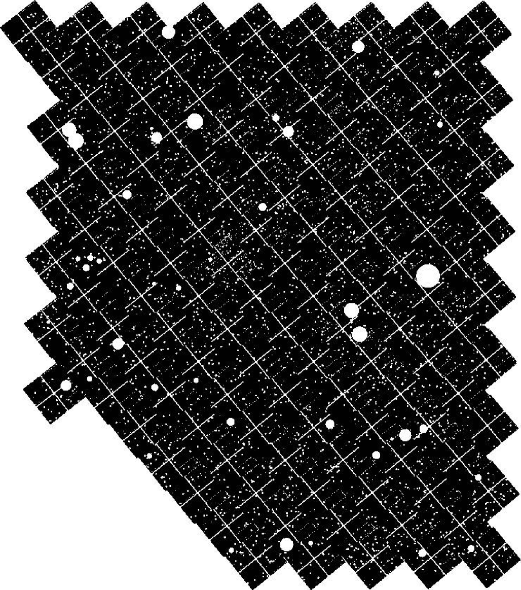
Figure 1: Default mosaic mask, which is used to remove all resolved point and extended sources from the flux mosaic (Eq. 4).

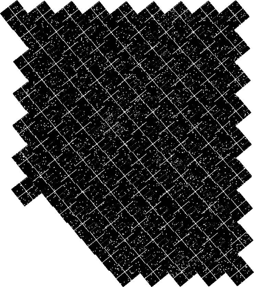
Figure 2: Special mosaic mask, which is used to remove only resolved point sources from but retain resolved extended sources in the flux mosaic (Eq. 4).

2.2.1 Construction

In order to measure CXB fluctuations at angular scales larger than ACIS-I’s FOV ($>17\arcmin$), we have to analysis the mosaic image of 126 ACIS-I observations. At first we construct the mosaics $\mathbb{E}$, $\mathbb{M}$, and $\mathbb{C}$ out of the individual exposure maps (E), masks (M), and background-subtracted count maps (C), respectively, for each energy band. Note that before the mosaics are constructed the exposure and count map of each observation are multiplied with its FOV mask (Section 2.1.2). With these mosaics we compute the flux mosaic for a given energy band as:

$$\mathbb{F}=\mathbb{M}\cdot\dfrac{\mathbb{C}}{\mathbb{E}}\text{ .}$$ (4)

Hence, the fluctuation mosaic is computed as:

$$\delta\mathbb{F}=\mathbb{F}-\left\langle\mathbb{F}\right\rangle\text{ ,}$$ (5)

where the mean flux mosaic is:

$$\langle\mathbb{F}\rangle=\mathbb{M}\cdot\dfrac{\Sigma_{i,j}\,F}{\Sigma_{i,j}\,M}\text{ .}$$ (6)

Here and in the following, blackboard bold characters ($\mathbb{M}$) represent mosaics, while bold italic characters (M) represent individual maps, and italic characters ($M$) represent individual image pixels of either a mosaic or a map (depending on the context). Our construction method ensures that overlapping regions of adjacent observations ($\sim 5\,\%$) are properly taken into account (also see Appendix C.4).

Note that the fluctuation mosaic is created with an image-pixel-binning factor of $b=32$, while individual fluctuation maps ($\delta\textit{{F}}$, Eq. 8 of Paper I), which are used to compute the stacked power spectrum, are created at the highest possible angular resolution of ACIS-I (image-pixel-binning of $b=1$). Hence, the former has a image-pixel-size of $15.744\arcsec$, while the latter have an image-pixel-size equal to the chip-pixel-size of ACIS-I, which is $\Delta p=0.492\arcsec$. Using a reduced angular resolution for the mosaic image makes our data analysis significantly faster and more manageable. To optimize the discrete Fourier transform computations of our analysis, the fluctuation mosaic is embedded in a squared image of $837\times 837$ image pixels ($\approx 3.66\times 3.66\,\mathrm{deg^{2}}$). Fluctuation maps are embedded in a squared image of $2\,900\times 2\,900$ image pixels ($\approx 23.8\times 23.8\,\mathrm{arcmin^{2}}$), which is large enough to contain an entire ACIS-I FOV.

2.2.2 Solid angle and flux

The solid angle of the mosaic mask ($\mathbb{M}$) is computed as

$$\Omega=(b\cdot\Delta p)^{2}\cdot\left(\Sigma_{i,j}\,M\right)\text{ ,}$$ (7)

The total solid angle covered by the mosaic image is $\approx 8.7\,\mathrm{deg^{2}}$, of which about $5\,\%$ are covered by two or more observations. When we apply our default mask shown in Figure 1, which removes all resolved sources, the remaining area reduces by about $5\,\%$ down to $\approx 8.3\,\mathrm{deg^{2}}$. For the special mask shown in Figure 2, which is produced from the default mask by retaining all resolved extended sources, the remaining area is $\approx 8.4\,\mathrm{deg^{2}}$. The average exposure time is $\approx 4.5$ ks (overlap corrected), which is $\sim 5\,\%$ higher than in Paper I due to the changes in the data processing (Section 2.1.2).

The average surface brightness of the flux mosaic ($\mathbb{F}$) is $0.77\pm 0.01\,\mathrm{counts\;s^{-1}\,deg^{-2}}$ in the $0.5-2.0\,\mathrm{keV}$ band after removing all resolved sources (default mask). This corresponds to $7.5\pm 0.1\,\times 10^{-12}\,\mathrm{erg\,cm^{-2}\,s^{-1}\,deg^{-2}}$ in physical units, which is $\sim 5\,\%$ smaller than in Paper I due to the changes in the data processing (Section 2.1.2). This discrepancy characterizes the amplitude of the systematic uncertainty of the absolute flux measurements in this work and in Paper I. If all resolved extended sources are retained on the image (special mask), the average surface brightness increases by $\sim 4\,\%$ to $0.80\pm 0.01\,\mathrm{counts\;s^{-1}\,deg^{-2}}$, which corresponds to $7.8\pm 0.1\,\times 10^{-12}\,\mathrm{erg\,cm^{-2}\,s^{-1}\,deg^{-2}}$. The difference between the flux computed with the special and default mask gives us the combined surface brightness of all resolved extended sources, which is $2.8\pm 0.8\,\times 10^{-2}\,\mathrm{counts\;s^{-1}\,deg^{-2}}$. This corresponds to $2.0\pm 0.6\,\times 10^{-13}\,\mathrm{erg\,cm^{-2}\,s^{-1}\,deg^{-2}}$ using the best-fit spectral model from Section 4.2.

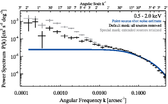
Figure 3: The measured power spectrum of the surface brightness fluctuations of the CXB in the $0.5-2.0\,\mathrm{keV}$ band for the default mask (black, Figure 1), where all resolved sources are removed, and for the special mask (gray, Figure 2), where in comparison to the default mask all resolved extended sources are retained. The blue curve represents our observational estimate of the point-source shot noise (Section 3.1) multiplied by the PSF-smearing model (Appendix B). The power spectra are adaptively binned.

3 Power spectrum of CXB fluctuations

We use the same formalism as in Paper I (section 4.1) to compute the power spectra of the mosaic image ($\delta\mathbb{F}$, Eq. 5) and of the average power spectrum of individual observations ($\delta\textit{{F}}$, Eq. 8 of Paper I). We will refer to the former as mosaic power spectrum ($P_{\mathrm{M}}(k)$) and to the latter as stacked power spectrum ($P_{S}(k)$).

The mosaic power spectrum covers angular scales from $\sim 32\arcsec$ up to about $3^{\circ}$ (angular frequencies $\sim 10^{-4}-0.0313\,\mathrm{arcsec^{-1}}$), where the maximal angular scale is determined by the geometry of the XBOOTES survey. The stacked power spectrum covers angular scales from $\sim 1\arcsec$ up to about $17\arcmin$ (angular frequencies $\sim 10^{-3}-0.300\,\mathrm{arcsec^{-1}}$), with the maximal angular scale determined by ACIS-I’s FOV. The minimal angular scale in both cases is defined by the Nyquist frequency ($k_{\mathrm{Ny}}=(2\,b\,\Delta p)^{-1}$), which depends on the image-pixel-binning used for the mosaic image ($b=32$) and for individual observations ($b=1$, Section 2.2.1). We combine the mosaic and stacked power spectra in order to cover the entire range of angular scales from $\sim 1\arcsec$ to $\sim 3^{\circ}$. This is done after subtraction of the photon shot noise (Appendix A). The two spectra are combined at the half of the Nyquist frequency of the mosaic power spectrum $k_{\mathrm{C}}=k_{\mathrm{Ny}}^{\mathrm{Mosaic}}/2\approx(63\arcsec)^{-1}\approx 0.016\,\mathrm{arcsec^{-1}}$. This choice of $k_{\mathrm{C}}$ is justified in Appendix C.6. The characteristics of all three power spectra are summarized in Table 2. For simplicity, in the following we will refer to the photon shot noise subtracted combined power spectrum as CXB power spectrum.

The CXB power spectrum in the $0.5-2.0\,\mathrm{keV}$ band is shown in Figure 3 for the default and special masks. For visualization purposes, we use adaptive binning in this and following plots. All fits of the power spectra were done to the unbinned data. As discussed in detail on Paper I, the CXB power spectrum has a significant contribution of the shot noise due to unresolved sources. It is shown in Figure 3 by the thick blue solid curve. Clustering and internal structure of unresolved sources leads to the deviations of the CXB power spectrum above the shot noise of unresolved sources. In the following, we will refer to any excess power above the shot noise of unresolved point sources $P_{\mathrm{PSSN}}$ as the LSS power spectrum $P_{\mathrm{LSS}}(k)$.

$$P(k)=\left(P_{\mathrm{LSS}}(k)+P_{\mathrm{PSSN}}\right)\,W_{\mathrm{PSF}}(k)$$ (8)

Note, that both $P_{\mathrm{LSS}}(k)$ and $P_{\mathrm{PSSN}}$ are affected by the smearing effect of Chandra’s point spread function ($W_{\mathrm{PSF}}(k)$, Appendix B), which leads to the decline of the power at high spatial frequencies.

3.1 Point-source shot noise

In order to study the LSS power spectrum the point-source shot noise needs to be subtracted from the CXB power spectrum (Eq. 8). It is an additive, scale-independent component, which arises from the fluctuation of the number of unresolved point-like sources (AGN and normal galaxies) per beam, similar to the photon shot noise (see section 4.3 of Paper I for a more detailed discussion). Unlike the photon shot noise it is however affected by the PSF-smearing.

In theory, the amplitude of the shot noise of unresolved point sources can be straightforwardly computed form the $\log N-\log S$ distribution of the unresolved sources (e.g. Eq. 18 of Paper I). However in practice, the theoretical prediction is subject to a number of uncertainties (section 5.1 of Paper I), of which one of the most significant is conversion from physical to instrumental units. For this reason we estimate the amplitude of the point-source shot noise directly from the CXB power spectrum itself. To this end, we compute the average power within the $5\arcsec-10\arcsec$ angular scale range and correct it for the PSF-smearing ($W_{\mathrm{PSF}}$, Appendix B):

$$\langle P_{(k_{1},k_{2})}\rangle=\frac{\Sigma_{k_{1}}^{k_{2}}P(k)}{\Sigma_{k_{1}}^{k_{2}}W_{\mathrm{PSF}}(k)}\text{ .}$$ (9)

where, $k_{1}$ and $k_{2}$ are the lower and upper limit of the considered angular scale range. From this calculation we obtain the point-source shot noise level of $2.5\pm 0.1\times 10^{-5}\,\mathrm{(cts\,s^{-1})^{2}\,deg^{-2}}$ in the $0.5-2.0\,\mathrm{keV}$ band. This value is consistent with the one obtained in Paper I. The so computed point-source shot noise contribution is shown in Figure 3 by the blue curve.

In Figure 4 we compare this value (gray horizontal bar) with theoretical predictions based on different $\log N-\log S$ of extragalactic point sources in the $0.5-2.0\,\mathrm{keV}$ band from the literature. In this figure, the theoretical shot noise level is plotted as function of the photon index of the power law, assumed in converting the energy flux to instrumental units. We can see that theoretical predictions agree with our measurement if we assume the effective average photon index of unresolved extragalactic point sources of $\Gamma\sim 1.6-1.7$. These values are somewhat lower than the best fit value of $\Gamma=1.73\pm 0.03$ obtained in Paper I (section 3.1.3) from the power law fit to the energy spectrum of the unresolved extragalactic emission in XBOOTES in the $0.5-10.0\,\mathrm{keV}$ band. We consider this agreement satisfactory, given the number of uncertainties involved in the measurement of the point-source shot noise level and in the theoretical calculation. Finally we note that Galactic absorption ($N_{\mathrm{H}}=10^{20}\,\mathrm{cm^{-2}}$) is always taken into account for the power law model.

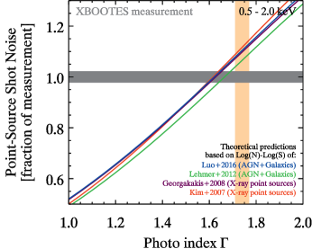
Figure 4: Comparison of the measured point-source shot noise level in the CXB power spectrum in the $0.5-2.0\,\mathrm{keV}$ band (gray horizontal bar, which thickness corresponds to one standard deviation) with theoretical predictions based on different $\log N-\log S$ of extragalactic point sources from the literature (solid curves, computed according to Eq. 18 of Paper I, Kim et al., 2007; Georgakakis et al., 2008; Lehmer et al., 2012; Luo et al., 2017) as a function of the photon index of the power law, assumed in converting the energy flux to instrumental units. The vertical shaded region shows the $1\sigma$ confidence interval for the slope of the power law – best fit in the $0.5-10.0\,\mathrm{keV}$ band to the unresolved extragalactic emission in XBOOTES. See Section 3.1 for discussion.

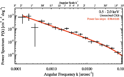
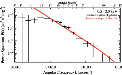
Figure 5: The power spectrum of the unresolved CXB (left panel) and of resolved extended sources (right panel) in the $0.5-2.0\,\mathrm{keV}$ band. The red lines show the best-fit power law model in the angular scale range $10\arcsec-20\arcmin$ multiplied by the PSF-smearing model (Appendix B). The power spectra are adaptively binned.

4 The LSS power spectrum

We defined the LSS power spectrum ($P_{\mathrm{LSS}}(k)$) as the excess power above the shot noise of unresolved point sources ($P_{\mathrm{PSSN}}$). $P_{\mathrm{LSS}}(k)$ is computed by subtracting $P_{\mathrm{PSSN}}$ from the CXB power spectrum and describes structure and correlation properties of unresolved sources. We can also compute the power spectrum of resolved clusters of galaxies $P_{\mathrm{rCG}}(k)$ by subtracting the CXB power spectrum computed with the default mask (all resolved sources masked out) from that of the special mask (only resolved point sources masked out). It describes the internal structure and cross correlation of resolved clusters of galaxies.

In Figure 5 we present our measurement of the LSS power spectrum of the unresolved CXB and of resolved clusters of galaxies. In both cases the power spectra have a power law shape in a rather broad range of angular frequencies exceeding two orders of magnitude. However, the slopes of the power spectra are significantly different, with the unresolved CXB power spectrum being significantly flatter. The power law fits $P(k)\propto k^{-\alpha}$ to these spectra gives best-fit values of slope $\alpha=0.96\pm 0.06$ and $\alpha=1.76\pm 0.04$ for the unresolved CXB and resolved clusters of galaxies, respectively. Note, that the best-fit values depend on the survey area and depth. There were determined via an $\chi^{2}$ minimization (using MPFIT from Markwardt, 2009) in the $10\arcsec-20\arcmin$ angular scale range. Also, the power spectrum of resolved clusters of galaxies has a clear flattening at low frequencies corresponding to angular scales larger than $\sim 20\arcmin-30\arcmin$.

4.1 Resolved clusters of galaxies

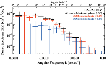
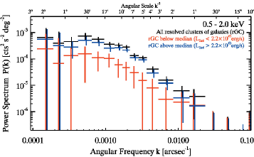
Figure 6: The power spectrum of resolved clusters of galaxies for different redshift (left) and luminosity groups (right).

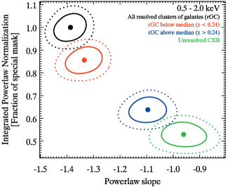
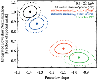
Figure 7: Best-fit parameters for the power law fit to the power spectrum of different redshift (left) and luminosity groups (right) of resolved clusters of galaxies. The corresponding power spectra are shown in Figure 6. Solid ellipses represent one standard deviation and dashed ellipses show the $90\,\%$ confidence level of a two parameter fit. The power law normalization is obtained by integrating the model over the angular scale range $10\arcsec-20\arcmin$ and is shown in the units of $\mathrm{counts^{2}\,s^{-2}\,deg^{-3}}$.

4.1.1 Redshift and luminosity dependence

Thanks to the work of Vajgel et al. (2014), we know the redshifts and luminosities of $\approx 72\,\%$ (31) of resolved extended sources detected in the XBOOTES field. Their median values are $z\approx 0.24$ and $L_{0.1-100\,\mathrm{keV}{}}\approx 2.2\times 10^{43}\,\mathrm{erg\;s^{-1}}$, respectively. With these values, we estimate a DMH mass of $M_{500}\approx 1.0\times 10^{14}\,\mathrm{M_{\sun}}\,h^{-1}$ and an ICM temperature of $T\approx 2.2$ keV, using the luminosity-mass relation of Anderson et al. (2015) and the luminosity-temperature relation of Giles et al. (2016, see Section 4.2.1 for the spectral model), respectively. Based on this we compute the $0.5-2.0\,\mathrm{keV}$ band luminosity of $L_{0.5-2.0\,\mathrm{keV}{}}\approx 1.2\times 10^{43}\,\mathrm{erg\;s^{-1}}$.

We use the median values to divide the sample of resolved clusters of galaxies into two groups in redshift and luminosity, separated by their median values, and plot their power spectra in Figure 6. In Figure 7 we plot best-fit parameters of the LSS power spectra ($P_{\mathrm{LSS}}(k)$) approximation with the power law model. In this calculation we excluded resolved extended sources without redshift and luminosity information. These figures demonstrate that the power spectrum of resolved clusters of galaxies is dominated by the nearby or the most luminous objects.

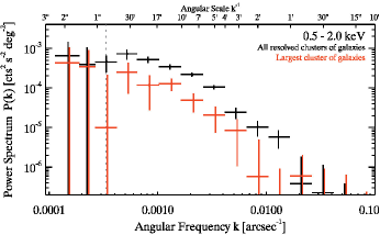
Figure 8: The power spectrum in the $0.5-2.0\,\mathrm{keV}$ band for all resolved clusters of galaxies (black, same as right panel of Figure 5) and for only the largest cluster (red). The gray dotted vertical line indicates the diameter of the circular exclusion area of the largest cluster.

4.1.2 Low frequency break

There is a definitive low frequency break in the power spectrum of resolved clusters of galaxies (right panel of Figure 5) at angular scales of $\sim 20\arcmin-30\arcmin$. At lower frequencies the power spectrum becomes flat implying that there is no correlation between surface brightness variations at the locations separated by angles larger than $\sim 20\arcmin-30\arcmin$. In Appendix C.3 we demonstrate with randomized observations that the low frequency break is real and is not of instrumental origin.

The break location and the shape of the power spectrum near the break characterizes the structure of ICM in the largest (in terms of the angular size) cluster of galaxies. In the XBOOTES field, this is XBS06 (Table 1 of Vajgel et al. 2014; J142657.9+341201 in Table 1 of K05) located in the the observation 4224. In Figure 8 we show the power spectrum of this cluster of galaxies (red). It was computed as a difference of the power spectra of the entire XBOOTES field with this cluster retained or masked out. In this calculation we set the radius of the circular exclusion area for XBS06 to be $25\arcmin$.

The power spectrum of XBS06 has the low frequency break at angular scales of $\sim 30\arcmin$, similar to the power spectrum of all resolved clusters of galaxies. The redshift of XBS06 is $z\approx 0.128$ (Vajgel et al., 2014). For this redshift, the angular scale of $\sim 30\arcmin$ corresponds to the linear scale of $\sim 3\,\mathrm{Mpc}\,h^{-1}$. Given the size of the galaxy cluster ($R_{500}=(0.59-0.65)\,\mathrm{Mpc}\,h^{-1}$, Vajgel et al., 2014, Table 3), this suggest that our fluctuation measurement is sensitive to the ICM structure up to the radius of $\sim 3\times R_{500}$.

This further justifies the claim of the Paper I that CXB fluctuation analysis can be efficiently used to study the average ICM structure in the outskirts of clusters of galaxies, out to their virial radii. Such studies are difficult and expensive to perform with conventional deep pointed observations of individual clusters, especially for a large number of objects, and are typically biased towards relatively nearby sources ($z\lesssim 0.1$, e.g. Eckert et al., 2012, 2017).

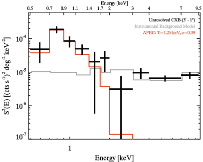
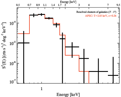
Figure 9: The energy spectrum $S^{2}(E)$ of fluctuations of the unresolved CXB (left panel) and of resolved clusters of galaxies (right panel). The best fit APEC models are shown by red histograms. The gray histogram on the left panel show the residual instrumental background spectrum with the best fit normalization. See Section 4.2 for details.

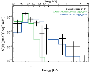
Figure 10: The energy spectrum $S^{2}(E)$ of fluctuations of the unresolved CXB (after subtracting the instrumental background model) in comparison to typical spectral models of AGN and normal galaxies (blue histogram), and of Galactic diffuse emission (green histogram).

4.2 Energy spectrum of fluctuations

The energy spectrum of angular fluctuations gives further insights to their origin. We characterize it with the energy dependence of the average power in the angular scale range of interest. In analogy with conventional energy spectra, this quantity is further normalized to the square of width of the energy range:

$$S^{2}(E)=\frac{\langle P(k_{1},k_{2})\rangle}{(\Delta E)^{2}}\text{ ,}$$ (10)

where $\langle P_{(k_{1},k_{2})}\rangle$ is defined in Eq. (9). The so defined $S^{2}(E)$ has the meaning of the squared spectral flux with units of $\mathrm{(counts\,s^{-1})^{2}\,deg^{-2}\,keV^{-2}}$. For the angular scale range in Eq. (10) we chose $3\arcmin-1^{\circ}$, which is a compromise between using as wide as possible range to achieve a high S/N and avoiding at the same time angular scales with potential systematic uncertainties.

The so obtained fluctuation spectra are plotted in Figure 9 for the unresolved CXB and resolved clusters of galaxies. Based on theoretical expectations and results of Paper I we approximate these spectra with the model of the emission of the optically thin plasma in collisional ionisation equilibrium (APEC model). To preserve the Gaussian statistics of errors we perform fitting in the squared spectral flux space, i.e. fit the quantity $S^{2}(E)$. To this end, we construct a grid of models in XSPEC and then compute $\chi^{2}$ and find the minimum and confidence intervals outside XSPEC. In the spectral fits we assume Galactic absorption with $N_{\mathrm{H}}=10^{20}\,\mathrm{cm^{-2}}$ and a metallicity of $0.3$ of the solar value.

There is an obvious hard tail in the energy spectrum of fluctuations of the unresolved CXB (left panel of Figure 9). This is a small residual left because of the imperfect subtraction of the instrumental background (Section 2.1.3 and Appendix C.2). To account for this residual background contribution we added to the model a component corresponding to the spectrum of the instrumental background which we adopt from Paper I and for which we keep the normalization free during the $\chi^{2}$ minimization. Note that the instrumental background component is absent in the energy spectrum of fluctuations of resolved clusters of galaxies, by the method of its construction, as it was computed as a difference of two power spectra having almost exactly same instrumental background contributions.

The best fit models are shown in Figure 9 and their confidence areas are plotted in Figure 11. The spectra of unresolved CXB fluctuations and of resolved clusters of galaxies are clearly different, with the former having lower temperature and originating at larger redshift, as it should be intuitively expected. This will be discussed in more detail in the next subsection.

In Figure 10 we compare the energy spectrum of fluctuations of unresolved CXB with other plausible models. The blue histogram shows an extragalactic power law with the photon index of $\Gamma=1.6$, which should be expected from unresolved AGN (Section 3.1). Such a spectrum is clearly much harder that the data, which is in good agreement with the Paper I. Same is true for any power law model with the photon index feasible for AGN and normal galaxies ($0<\Gamma<3$, e.g. Reynolds et al., 2014; Ueda et al., 2014; Yang et al., 2015).

The Galactic diffuse emission can be described on average with an unabsorbed ($N_{\mathrm{H}}=0\,\mathrm{cm^{-2}}$) APEC model with temperatures below $T\sim 0.30$ keV (e.g. Lumb et al., 2002; Hickox & Markevitch, 2006; Henley & Shelton, 2013). An APEC model with $T=0.30$ keV is shown as green histogram in Figure 10. Obviously, it is much softer than the observed spectrum. It is possible, however, that the lowest energy band ($0.5-0.7\,\mathrm{keV}$) may contain some contribution from the diffuse emission of the Galaxy.

We also tested a more complex, two-component model, where we use an unabsorbed APEC model ($N_{\mathrm{H}}=0\,\mathrm{cm^{-2}}$) to describe the Galactic diffuse emission and a power law ($N_{\mathrm{H}}=10^{20}\,\mathrm{cm^{-2}}$) to describe unresolved AGN and normal galaxies. It is the same model as used to describe the unresolved CXB emission of XBOOTES (section 3.1 of Paper I). The best-fit APEC temperature and photon index of such a model are inconsistent with previous measurements for the Galactic and extragalactic components, although errors are large due to poor resolution and low S/N of the energy spectrum. Further, our best-fit model of the unresolved CXB emission of XBOOTES (Table 2 of Paper I) is excluded by more than $3\sigma$. Due to these reasons, we limit our discussion to single-component models.

Table 1: Comparison of the best-fit values of the energy spectrum of CXB fluctuations (Figure 11) with theoretical expectations for unresolved and resolved clusters of galaxies.

	Unresolved(a)	Resolved(b)
Redshift z:
Best-fit of observation (Figure 9)	$0.39^{+0.10}_{-0.21}$	$0.26^{+0.28}_{-0.05}$
Best-fit of simulation(c)	0.41	-
Flux-weighted mean	0.35	0.23
Median	0.49	0.24
Temperature T (keV):
Best-fit of observation (Figure 9)	$1.25^{+0.35}_{-0.20}$	$2.05^{+0.50}_{-0.25}$
Best-fit of simulation(c)	1.1	-
Flux-weighted mean	1.4	2.4(d)
Median	1.1	2.2(d)
Luminosity $L_{0.5-2.0\,\mathrm{keV}{}}$ ($10^{43}\,\mathrm{erg\;s^{-1}}$):
Derived(d) from best-fit of observation	$0.3^{+0.3}_{-0.1}$	$1.0^{+1.1}_{-0.4}$
Derived(d) from best-fit of simulation	0.2	-
Flux-weighted mean	0.3	1.4
Median	0.2	1.2
DMH mass $M_{500}$ ($10^{14}\,\mathrm{M_{\sun}}\,h^{-1}$):
Derived(e) from best-fit of observation	$0.4^{+0.3}_{-0.1}$	$1.1^{+0.5}_{-0.3}$
Derived(e) from best-fit of simulation	0.4	-
Flux-weighted mean	0.5(e)	1.0(f)
Median	0.3(e)	0.9(f)

(a) Flux-weighted mean and median values are computed using the XLF of Pacaud et al. (2016) assuming an upper flux limit of $S_{0.5-2.0\,\mathrm{keV}}=3\times 10^{-14}\,\mathrm{erg\,cm^{-2}\,s^{-1}}$ and a lower temperature limit of $T=0.4$ keV (see Section 2.1.5 for details). (b) Flux-weighted mean and median values are derived from the catalog of Vajgel et al. (2014, see our Section 4.1.1 for details). (c) Simulated energy spectrum of unresolved clusters of galaxies (see Section 4.2.1 for details). (d) Using the luminosity-temperature scaling relation of Giles et al. (2016). (e) Using the mass-temperature scaling relation of Lieu et al. (2016). (f) Using the luminosity-mass scaling relation of Anderson et al. (2015).

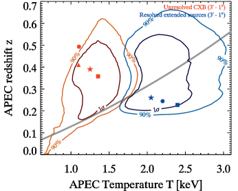
Figure 11: Confidence regions for the APEC model parameters for energy spectra of fluctuations of unresolved CXB (red contours) and for resolved clusters of galaxies (blue contours). The stars show corresponding best-fit values, the squares and circles show the expected flux-weighted mean and median values for each spectrum, computed as described in Section 4.2.1 and summarized in Table 1. The red triangle shows the best-fit value for the simulated energy spectrum of unresolved clusters of galaxies. The gray curve shows the maximal redshift at which clusters of galaxies of a given temperature can be detected in XBOOTES, assuming that their luminosities obey the luminosity-temperature scaling relation of Giles et al. (2016).

4.2.1 Comparison with theoretical expectations

As a consistency check, we compare the best-fit spectral parameters for resolved clusters of galaxies with the actually measured values in the XBOOTES field. We will use the redshift and luminosity measurements from Vajgel et al. (2014) and compute the flux-weighted mean and median values for resolved clusters of galaxies. Based on these values we compute the expected ICM temperature using the luminosity-temperature scaling relation of Giles et al. (2016, Table 2). The result of this calculation is summarized in Table 1 and shown in Figure 11 as a blue rectangle and circle. As one can see, they are quite close to the best-fit value (blue star), although the size of the error region is rather big, due to the limited S/N of the data.

For unresolved CXB the expected flux-weighted mean and median values are derived from the redshift, luminosity and ICM temperature distributions of the unresolved clusters of galaxies, which are computed using the XLF $\Phi$ of Pacaud et al. (2016) assuming an upper flux limit of $S_{0.5-2.0\,\mathrm{keV}}=3\times 10^{-14}\,\mathrm{erg\,cm^{-2}\,s^{-1}}$ and a lower temperature limit of $T=0.4$ keV (see Section 2.1.5 for details). For the redshift and luminosity distribution we are using Eqs. (10) and (11) of Paper I, while for the ICM temperature distribution we are using:

$$\frac{\mathrm{d}S(T)}{\mathrm{d}T}= \int\!\mathrm{d}z\;\Phi\!\left(L_{r}(T,z),z\right)\;L_{r}^{\prime}(T,z)\;\frac{\mathrm{d}^{2}V(z)}{\mathrm{d}z\mathrm{d}\Omega}$$

$$\times\;S[L_{r}(T,z),z]\;\left[1-f(S[L_{r}(T,z),z])\right]\text{,}$$ (11)

which is the flux production rate per solid angle as a function of temperature. $L(T,z)$ and $L^{\prime}(T,z)$ are the luminosity-temperature scaling relation of Giles et al. (2016) and its first derivative, respectively. All other quantities are described in section 3.3 of Paper I. The result is summarized in Table 1 and shown in Figure 11 as the red rectangle and circle.

One can see that the flux-weighted mean (red square in Figure 11) is located within $1\sigma$ contour while the median value (red circle) is outside the $90\,\%$ confidence area (but still within $2\sigma$ contour). This discrepancy is not critical given that the observed spectrum is a linear combination of multiple APEC models with different temperatures and redshifts. We therefore simulated the expected energy spectrum of unresolved clusters of galaxies based on their XLF. To this end we constructed a grid of $15\times 15$ cells covering the relevant parameter ranges on the redshift-temperature plane. For each cell on the grid we computed the APEC model, which normalisation was determined according to the XLF of clusters of galaxies, using the luminosity-temperature scaling relation of Giles et al. (2016). The K-corrected emission spectra of all cells were summed to obtain the theoretical spectrum of unresolved clusters of galaxies, which was then fit with a single temperature APEC model, similar to the observed one (Figure 9). The best-fit parameters of this simulation are shown in Figure 11 with the red triangle. As one can see, it is consistent with the best-fit values of the temperature and redshift of the observed spectrum of CXB fluctuations within $1\sigma$ contour.

Based on the best-fit parameters of the observed energy spectrum (Figure 9), we can derive for the unresolved clusters of galaxies in XBOOTES a characteristic luminosity of $L_{0.5-2.0\,\mathrm{keV}{}}=3^{+3}_{-1}\times 10^{42}\,\mathrm{erg\;s^{-1}}$ and DMH mass of $M_{500}=4^{+3}_{-1}\times 10^{13}\,\mathrm{M_{\sun}}\,h^{-1}$. For the latter we use the mass-temperature scaling relation of Lieu et al. (2016).

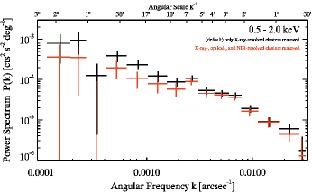
Figure 12: Comparison of the power spectrum of the unresolved CXB, when additionally optically identified or NIR candidates of clusters of galaxies are removed. These sources were taken from catalogs listed in Section 4.3. The corresponding mask is shown on the left of Figure 13.

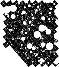
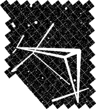
Figure 13: Mosaic masks used to constrain the combined contributions of optical and NIR clusters of galaxies (left, see Section 4.3) and filaments between X-ray-resolved clusters of galaxies (right, see Section 4.4). They are based on the default mask (Figure 1).

4.3 Contribution of optically- and NIR-identified clusters of galaxies

In this section we will investigate the contribution of clusters of galaxies identified in the XBOOTES field at other wavelengths. To this end we will be excluding from the analysis the image areas around known clusters of galaxies and computing the power spectrum of unresolved CXB, comparing the result with our default mask. We will use the following catalogs:

1. The SDSS-DR12 catalog by Tempel et al. (2017). It contains clusters of galaxies below redshift $z=0.2$ and brighter than $r=17.77$. About 150 of their objects are within the area of XBOOTES survey. These sources are removed with a circular exclusion area with a radius equal to half of their $R_{200}$.

2. The SDSS-DR6 catalog by Szabo et al. (2011). This catalog contains clusters of galaxies in the redshift range of $0.1<z<0.7$ with the lower magnitude limit of $r=22.0$ ($>90\,\%$ completeness). About 120 of their objects are within the area of XBOOTES. Sources are removed with a circular exclusion area with the radius equal to half of their $R_{200}$.

3. A catalog of cluster candidates of Eisenhardt et al. (2004) from the Spitzer/IRAC shallow survey (ISCS) of NDWFS. The survey has the aperture-corrected 5$\sigma$ depth of $\approx 19.1$ and $18.3$ mag (Vega) at 3.6 and 4.5 $\mu$m, respectively. It contains objects up to redshift $z=2.2$ and about 330 of them are within the area of XBOOTES. We used a circular exclusion region of a constant radius of $400\,\mathrm{kpc}\,h^{-1}$, since their physical sizes are unknown. This value is approximately equal to the median $R_{200}/2$ of the selected SDSS-DR6 sources, $\sim 2.5$ times larger than the median $R_{200}/2$ of the selected SDSS-DR12 sources, and $\sim 30\,\%$ larger than the median $R_{500}$ of 14 X-ray-resolved clusters of galaxies in XBOOTES obtained by Vajgel et al. (2014, Table 3).

These catalogs were used to amend our default mask, and the resulting mask is shown on the left of Figure 13. The power spectrum is shown in Figure 12 along with our nominal power spectrum of the unresolved CXB obtained with the default mask. One can see that, although the exclusion of the selected clusters does have some effect on the power spectrum, they can not explain the amplitude of observed fluctuations of unresolved CXB. This suggests that the used catalogs may be not deep and/or complete enough to account for the observed fluctuations.

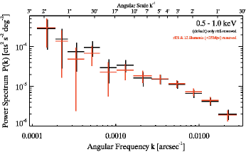
Figure 14: The power spectrum of the unresolved CXB in the $0.5-1.0\,\mathrm{keV}$ band, where filaments between resolved clusters of galaxies are retain (black, default) and removed (red). The corresponding mask for the latter is shown in Figure 13 on the right.

4.4 WHIM

Due to its low temperature ($\sim 10^{5}-10^{7}\,\mathrm{K}\lesssim 1\,\mathrm{keV}$, see e.g. review of Bregman, 2007), WHIM is not expected to make any significant contribution to the fluctuations of unresolved CXB in the most of the energy range considered in this work. In agreement with this, the energy spectrum of CXB fluctuations (Section 4.2) is adequately described by the emission spectrum of optically thin plasma with the temperature of $1.3^{+0.4}_{-0.2}$ keV, and does not require any softer spectral component. This temperature is obviously too high to be associated with WHIM. On the other hand, our current measurement can not exclude some contribution of WHIM in the softest energy band ($0.5-0.7\,\mathrm{keV}$).

Some hot gas may be found in the filaments between clusters of galaxies, as cosmological hydrodynamical simulations predict and very deep XMM-Newton observations have shown for single cases (e.g. Cen & Ostriker, 2006; Werner et al., 2008; Roncarelli et al., 2012; Nevalainen et al., 2015). To constrain contribution of such filaments associated with resolved clusters of galaxies we identify among the latter all pairs of clusters separated by the comoving distance smaller than $25\,\mathrm{Mpc}\,h^{-1}$. This is a rather conservative upper limit on the filament length (e.g. Tempel et al., 2014). We mask out all the regions on the mosaic image connecting such pairs of clusters, in addition to all resolved sources excluded by the default mask. The filament regions have a trapezoidal form, which width at each end equals to the angular size of the cluster of galaxies it is connected to. For the angular size of a cluster of galaxies we used the diameter of its circular exclusion area of the default mask (i.e. $2\times(6\times\text{rES-size})$). The resulting power spectrum in the $0.5-1.0\,\mathrm{keV}$ band is shown in Figure 14 along with our standard LSS power spectrum obtained with the default mask. As one can see from this plot, the possible filaments of gas connecting resolved clusters of galaxies do not make a significant contribution to the power spectrum of unresolved CXB. The same can be concluded from the comparison of the average power (Eq. (9), for $3\arcmin-1^{\circ}$) for the lowest energy band ($0.5-0.7\,\mathrm{keV}$) for both masks.

5 Summary

Surface brightness fluctuations of CXB carry unique information about faint source populations, which are unreachable via conventional approach based on studies of resolved sources. Accessing these information via angular correlation studies has become a new frontier of LSS research with X-ray surveys, successfully complementing conventional studies (e.g. Cappelluti et al., 2012, 2013; Helgason et al., 2014; Mitchell-Wynne et al., 2016; Kolodzig et al., 2017).

We studied fluctuations of the X-ray surface brightness in the XBOOTES field. With its area of $\approx 9$ deg² it is the largest contiguous Chandra survey which has been observed to the $\approx 5$ ksec depth. We constructed mosaic images of the entire XBOOTES field in various energy bands and, after masking out resolved sources (point-like and extended), computed power spectra covering the range of angular scales from $\approx 2\arcsec$ to $\approx 3^{\circ}$. This extends by more than an order of magnitude the largest angular scales investigated in Paper I where stacked power spectra computed over individual Chandra observations were analyzed. After subtracting the contribution of unresolved point sources (the so called point-source shot noise) we obtained the power spectrum of fluctuations of unresolved CXB. We also computed power spectrum of the mosaic image in which only resolved point sources were masked out while all extended sources were left on the image. The difference between the latter and the power spectrum of unresolved CXB represents the power spectrum of resolved clusters of galaxies (see footnote 8 regarding identification of resolved extended sources with clusters of galaxies). These results present the most accurate CXB fluctuation measurement to date at angular scales below $\sim 3^{\circ}$.

In the power spectrum of unresolved CXB, the non-trivial LSS signal dominates the shot noise of unresolved point sources at all angular scales above $\sim 1\arcmin$. As it was demonstrated in Paper I, this signal is mainly due to CXB brightness fluctuations caused by unresolved clusters and groups of galaxies.

The main results of this work can be summarized as follows:

1. There is a clear difference in shape between power spectra of unresolved CXB and resolved clusters of galaxies. While the former has an approximate power law shape with the slope of $\Gamma=0.96\pm 0.06$ in the entire range of angular scales, the latter is significantly steeper, with $\Gamma=1.76\pm 0.04$, and has a clear low frequency break at the angular scale of $\sim 30\arcmin$. The location of the low frequency break suggests that this analysis is sensitive to the ICM structure out to $\sim 3\times R_{500}$ ($\sim 3\,\mathrm{Mpc}\,h^{-1}$, Section 4.1). Thus, CXB fluctuations carry information about the average ICM structure at large radii, out to the virial radius.

2. From the power spectra computed in a number of narrow energy bands we constructed the energy spectrum of fluctuations using the approach similar to the Fourier-frequency resolved spectroscopy proposed by Revnivtsev, Gilfanov & Churazov (1999) to study spectral variability of X-ray binaries. The energy spectra ($0.5-10.0\,\mathrm{keV}$) of fluctuations of the unresolved CXB and of resolved clusters of galaxies are well described by the redshifted emission spectrum of optically thin plasma, as it should be for ICM emission. For fluctuations of unresolved CXB we obtained the best-fit temperature of $T=1.3^{+0.4}_{-0.2}\,\mathrm{keV}$ and the redshift of $z=0.4^{+0.1}_{-0.2}$. These numbers are consistent with theoretical expectations based on the XLF of clusters of galaxies and scaling relations for the parameters characterizing their X-ray emission. The DMH mass corresponding to the best-fit parameters is $M_{500}=4^{+3}_{-1}\times 10^{13}\,\mathrm{M_{\sun}}\,h^{-1}$ and the luminosity is $L_{0.5-2.0\,\mathrm{keV}{}}=3^{+3}_{-1}\times 10^{42}\,\mathrm{erg\;s^{-1}}$. For resolved clusters we obtained $T=2.1^{+0.5}_{-0.3}\,\mathrm{keV}$ and $z=0.3^{+0.3}_{-0.1}$, which is in agreement with the redshift and ICM temperature of resolved clusters of galaxies in XBOOTES. As expected, fluctuations of unresolved CXB are caused by cooler (i.e. less massive) and more distant clusters and groups of galaxies.

3. Comparison with the available catalogs of clusters of galaxies covering the XBOOTES field suggests that they may be not deep and/or complete enough to account for the observed fluctuations. We also did not find clear evidence for contribution of WHIM to the observed fluctuations of the CXB surface brightness.

Our results demonstrate the significant diagnostic potential of angular correlation analysis of CXB fluctuations in order to study the ICM structure in clusters of galaxies.

Appendix A Photon shot noise

The photon shot noise ($P_{\mathrm{Phot.SN}}$) is an additive, scale-independent component of the power spectrum, which arises from the fluctuation of the number of photons per beam. Since we are using instrumental-background-subtracted count maps C (Eq. 1), we have to take into account the photon shot noise of the total-count maps ($\textit{{C}}^{\mathrm{Total}}$) and of the instrumental-background maps ($\textit{{C}}^{\mathrm{BKG}}$, Eq. 2). Since both are uncorrelated, we can estimated their photon shot noise separately and add them up:

$$P_{\mathrm{Phot.SN}}=P_{\mathrm{Phot.SN}}^{\mathrm{Total}}+P_{\mathrm{Phot.SN}}^{\mathrm{BKG}}\text{ .}$$ (12)

For the stacked power spectrum we are using the analytical estimator to estimate the photon shot noise for both types of maps:

$$P_{\mathrm{Phot.SN}}^{\mathrm{Total}}=\dfrac{1}{\Omega}\sum_{j}^{N}\dfrac{C^{\mathrm{Total}}_{j}}{E_{j}^{2}}\text{ ,}$$ (13)

$$P_{\mathrm{Phot.SN}}^{\mathrm{(BKG)}}=\dfrac{1}{\Omega}\sum_{j}^{N}\dfrac{C_{j}^{\mathrm{Stow}}\cdot S_{j}^{2}}{E_{j}^{2}}\text{ .}$$ (14)

For simplicity we use here a single index ($j$) for the summations over all image pixels $N$ of a 2D quantity. $C_{j}^{\mathrm{Total}}$, $C_{j}^{\mathrm{Stow}}$, $E_{j}$, and $S_{j}$ are pixels of the maps $\textit{{C}}^{\mathrm{Total}}$, $\textit{{C}}^{\mathrm{Stow}}$, E, and S, respectively. The stowed background map${}^{\ref{StowedBKG}}$ ($\textit{{C}}^{\mathrm{Stow}}$) is the same for all observation, while the map S of each observation has the rescaling factor $S$ (Eq. 3) as a constant value. The analytical estimator is explained and discussed in Paper I (appendix C), where we also show its derivation.

For the mosaic power spectrum we are using the analytical estimator for the photon shot noise of the total-count mosaic ($\mathbb{C}^{\mathrm{Total}}$). In this respect, $C_{j}^{\mathrm{Total}}$ and $E_{j}$ in Eq. (13) are pixels of the mosaics $\mathbb{C}^{\mathrm{Total}}$ and $\mathbb{E}$, respectively, which are constructed out of the maps $\textit{{C}}^{\mathrm{Total}}$ and E. The instrumental-background mosaic $\mathbb{C}^{\mathrm{BKG}}$ is constructed out of the maps: $(\textit{{C}}^{\mathrm{Stow}}\cdot\textit{{S}}^{2})$. Since $\textit{{C}}^{\mathrm{Stow}}$ is the same for all observation, the analytically estimator (Eq. 14) overestimates significantly the photon shot noise (e.g. $\gtrsim 10\,\%$ in the $0.5-2.0\,\mathrm{keV}$ band). Hence, for the instrumental-background mosaic we are using the high-frequency estimator, where we estimate the photon shot noise from the average power of the frequency range $[k^{\mathrm{(HF)}}_{\mathrm{min}},k_{\mathrm{Ny}}^{\mathrm{Mosaic}}]$ with $k^{\mathrm{(HF)}}_{\mathrm{min}}=k_{\mathrm{Ny}}^{\mathrm{Mosaic}}\times 0.80\approx 0.025\,\mathrm{arcsec^{-1}}\approx(39\arcsec)^{-1}$. This is possible because for the chosen frequency range the photon-shot-noise-subtracted power spectrum of the stowed background map ($\textit{{C}}^{\mathrm{Stow}}$) is about two orders of magnitude smaller than the photon shot noise itself. The high-frequency estimator is explained and discussed in detail in Paper I (appendix C).

For the mosaic power spectrum the photon shot noise of the instrumental-background $P_{\mathrm{Phot.SN}}^{\mathrm{BKG}}$ contributes less than $1\,\%$ to the total photon shot noise (Eq. 12). Hence, given the shape and amplitude of our CXB power spectrum (Figure 3) only small angular scales below $\sim 1\arcmin$ of the mosaic power spectrum are affected by potential inaccuracies of the estimate of $P_{\mathrm{Phot.SN}}^{\mathrm{(BKG)}}$. In this respect, one should take in mind that our combined power spectrum (Section 3) only takes the mosaic power spectrum above $\sim 1\arcmin$ (below $k_{\mathrm{C}}=k_{\mathrm{Ny}}^{\mathrm{Mosaic}}/2\approx 0.016\,\mathrm{arcsec^{-1}}$) into account, which is a precaution in order to avoid the smallest angular scales of the mosaic power spectrum (Appendix C.6).

Note, that all shown power spectra in this work are already subtracted by the photon shot noise.

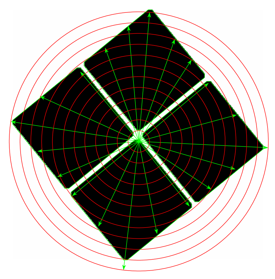
Figure 15: Sampling of ACIS-I’s FOV for the PSF-smearing model. Green arrows show the 20 azimuthal angles and red circles show the 13 offset angles ($\theta=0\arcmin-12\arcmin$, in $1\arcmin$-steps). PSF simulations were performed at positions, where green and red lines intersect within the black areas. See Appendix B for details.

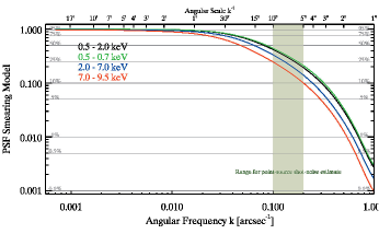
Figure 16: Our PSF-smearing model for selected energy bands. See Appendix B for details.

Appendix B PSF-smearing model

Given our change in the data preparation and processing in comparison to Paper I (Section 2.1), we also update our PSF-smearing model $W_{\mathrm{PSF}}(k)$ (for previous model see appendix B of Paper I), which is now computed for each energy band individually. For the PSF simulation we are using the CIAO tool simulate_psf in combination with the MARX software package (v5.3.1). We adjust the count rate in each band to achieve an on-axis pile-up probability below $\sim 1\,\%$. To still obtain a high S/N, we use an exposure time of $\sim 1.3$ Ms, which results in more than $\sim 2500$ counts per PSF simulation. We sample ACIS-I’s FOV with 20 azimuthal angles and 13 offset angles ($\theta=0\arcmin-12\arcmin$, in $1\arcmin$-steps). This results in 173 unique PSF positions within the FOV mask, as shown in Figure 15. We compute the power spectra of all PSF simulations and first average them over all azimuthal angles per offset angle before we compute the weighted average over all offset angles. For the weights we use the surface area times the average exposure time of the annulus ($1\arcmin$ wide) of each offset angle. This weighting is designed to also take the vignetting into account, although it appears to be almost neglectable effect. The resulting FOV-averaged PSF power spectrum $W_{\mathrm{PSF}}(k)$, alias our PSF-smearing model, is shown in Figure 16 for selected energy bands.

We can see from Figure 16 that the PSF-smearing is only important for angular scales below $\sim 1\arcmin$ and its impact increase with energy as expected given the energy dependence of Chandra’s PSF.

Appendix C Systematic effects

Below we discuss several systematic effects of our measurement of the CXB surface brightness fluctuations. Here, we focus primarily on the mosaic power spectrum since we already studied extensively the systematic effects of the stacked power spectrum in Paper I (appendix D).

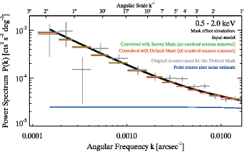
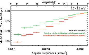
Figure 17: The impact of the mask effect on the mosaic power spectrum. Top: The convolved mosaic power spectra after the default mask (red) or the survey mask (green) was applied to a simulated image, which is based on the input model (black curve). Also show is the mosaic power spectrum of the original XBOOTES observations for the default mask (gray). Bottom: The ratio of the convolved mosaic power spectra to the input model. See Appendix C.1 for details.

C.1 Mask effect

The impact of the mask effect on the stacked power spectrum is shown in Paper I (appendix D1). We use the same procedure describe there to test the impact on the mosaic power spectrum by the default mask (Figure 1) and the survey mask, which is the mosaic of all FOV masks (Section 2.1.2). The input model follows Eq. (8) and consists of the best-fit powerlaw model of the LSS power spectrum for the default mask (left panel of Figure 5) plus the measured point-source shot noise (Section 3.1), which are both multiplied by our PSF-smearing model (Appendix B). We use 5000 iterations for our mask effect simulation and the resulting convolved mosaic power spectra are shown in Figure 17.

One can see that due the mask effect the mosaic power spectrum is suppressed by less than $\sim 20\,\%$ at the lowest considered frequency bin and at angular scales below $\sim 30\arcmin$ it is suppressed by less than $\sim 10\,\%$. Figure 17 also shows that the survey geometry of XBOOTES, represented by the survey mask (green), causes the largest suppression, while the additional removal of resolved sources, included in the default mask (red), increases the suppression only by less than $\sim 5\,\%$ in respect to the survey geometry. In any case, we can see in the top panel of Figure 17 that the suppression is much smaller than the statistical uncertainty of our measurement (gray), which makes the mask effect an almost negligible systematic effect (also see Appendix C.6). This is consistent with the conclusion for the stacked power spectrum shown in Paper I (appendix D1).

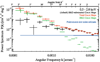
Figure 18: Comparison of the mosaic power spectra in the $0.5-2.0\,\mathrm{keV}$ band for the default mask based on three different count maps. In black we show our default power spectrum, where we use the instrumental-background-subtracted count maps C (Eq. 1). In red we show the power spectrum for the total-count maps $\textit{{C}}^{\mathrm{Total}}$, where the instrumental background was not subtracted. In green we show the power spectrum for the instrumental background maps $\textit{{C}}^{\mathrm{BKG}}$ (Eq. 2), which are all based on the same stowed background map $\textit{{C}}^{\mathrm{Stow}}$ normalized for each observation with a scaling factor $S$ (Eq. 3). See Section 2.1.3 and Appendix C.2 for details.

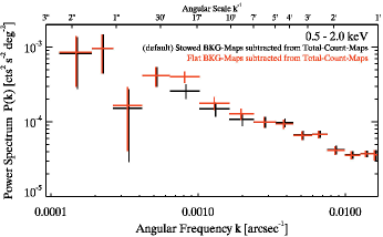
Figure 19: Comparison of the mosaic power spectra in the $0.5-2.0\,\mathrm{keV}$ band for the default mask based on two different methods of subtracting the instrumental background from the total-count maps ($\textit{{C}}^{\mathrm{Total}}$). In black we show our default method, where the scaled stowed background maps $\textit{{C}}^{\mathrm{BKG}}$ (Eq. 2) are used, and in red we show an alternative method, where flat background maps with the average surface brightness of $\textit{{C}}^{\mathrm{BKG}}$ of each observation as a constant value are used. See Appendix C.2 for details.

C.2 Instrumental background

In Figure 18 we compare the power spectra of two mosaics, which are constructed either with instrumental-background-subtracted count maps C (black, default, Eq. 1) or with total-count maps $\textit{{C}}^{\mathrm{Total}}$ (red, Section 2.1.3), for the $0.5-2.0\,\mathrm{keV}$ band for the default mask. Additionally, we show the power spectrum of the mosaic, which is constructed out of the instrumental background maps $\textit{{C}}^{\mathrm{BKG}}$ (Eq. 2). We can see in Figure 18 that when one uses total-count maps the power spectrum (red) above angular scales of $\sim 10\arcmin$ is dominated by fluctuations from the instrumental background (green). Such additional fluctuations are caused by the strong variation of the quiescent instrumental background between adjacent observations. Fortunately, such instrumental fluctuations can be removed by using instrumental-background-subtracted count maps.

In Figure 19 we present the power spectra of two mosaics, where we used two different methods of subtracting the instrumental background from the total-count maps ($\textit{{C}}^{\mathrm{Total}}$). Our default method is shown in black, where we use the scaled stowed background maps $\textit{{C}}^{\mathrm{BKG}}$ (Eq. 2) for the subtraction. An alternative method is shown in red, where we use flat background maps with the average surface brightness of $\textit{{C}}^{\mathrm{BKG}}$ of each observation as a constant value. The latter method has the advantage that it is much simpler to compute and that it does not increases the overall photon shot noise ($P_{\mathrm{Phot.SN}}^{\mathrm{(BKG)}}=0$) in comparison to our default method (Appendix A). We can see in Figure 19 that the alternative method works almost as good as our default method but for angular scales around $\sim 7\arcmin-\sim 20\arcmin$ is produces slightly higher power. This deviation arises from inhomogeneities of the instrumental background within the FOV, which are discussed in Paper I (appendix D2). They can only be corrected properly with the use of the scaled stowed background maps. However, the alternative method still appears sufficient, when one only likes to study fluctuations for angular scales at least twice as large as the FOV.

Note, that if one does not include those observations with a particular high instrumental background when constructing the mosaic, than the instrumental-background-subtraction would not be necessary at the given S/N of the power spectrum in the $0.5-2.0\,\mathrm{keV}$ band.

For energy bands above $\sim 3$ keV the instrumental fluctuations still dominate the power spectrum on large angular scales (see left panel of Figure 9), although instrumental-background-subtracted count maps are used. This arises from the fact that the effective area${}^{\ref{acisi_area}}$ of ACIS-I is significantly smaller at these energies in comparison to the $0.5-2.0\,\mathrm{keV}$ band, which results in a much smaller fraction of source counts in respect to instrumental background counts. In the $0.5-2.0\,\mathrm{keV}$ band the fraction is $52\pm 1\,\%$, while in the $2.0-7.0\,\mathrm{keV}$ the fraction is only $8.6\pm 0.3\,\%$. In the extreme regime, where less than one out of ten detected counts is an actual source count, our instrumental-background-subtraction method is apparently not accurate enough to remove instrumental fluctuations sufficiently well on large angular scales ($\lesssim 17\arcmin$). Fortunately, we can account for this in our energy spectrum analysis of the LSS power spectrum by including an instrumental background model in our a spectral model (Section 4.2).

We have already shown in Paper I (appendix D2) that for the stacked power spectrum we can neglected instrumental fluctuations for angular scales within ACIS-I’s FOV ($\lesssim 17\arcmin$) in the $0.5-2.0\,\mathrm{keV}$ band. We tested that this is also true with the data processing of this work (Section 2).

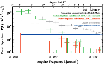
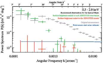
Figure 20: Comparison of the mosaic power spectrum for the original XBOOTES observations (gray), and randomized observations, where the surface brightness equals the surface brightness of the original observation (green) or of the original mosaic (red). Top: Default mask. Bottom: Special mask.See Appendix C.3 for details.

C.3 Test with randomized observations

To further test for instrumental fluctuations in the mosaic power spectrum we also compute the power spectra of mosaics constructed with randomized observations. These observations are at the same sky position as the original XBOOTES observations but they only contain counts with random sky coordinates, while the total number of counts is adjusted to a certain surface brightness. Hence, each randomized observation only contains Poisson noise. We create them for each mask and energy band separately. The randomization smooths out any fluctuations on angular scales below ACIS-I’s FOV ($\lesssim 17$), which is acceptable since in this experiment we are interested on fluctuations on larger angular scales. We compute the mosaic power spectrum for two cases: (a) the surface brightness of a single randomized observation equals the surface brightness of the XBOOTES observation at the same sky position, (b) the surface brightness of all randomized observations equals the surface brightness of the XBOOTES mosaic (Section 2.2.2). We would expect for (a) that the resulting mosaic power spectrum is in agreement with the original one on the largest angular scales ($\gtrsim 1^{\circ}$), and for (b) that the resulting mosaic power spectrum does not contain a signal at all (i.e. it is in agreement with the photon shot noise), for the case that the original mosaic power spectrum does not contain any additional instrumental signal due to its construction (Section 2.2.1). In Figure 20 we compare all three mosaic power spectra for the default mask (top panel) and special mask (bottom panel) and we can see that they indeed agree with our expectations.

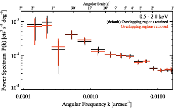
Figure 21: Comparison of the mosaic power spectra in the $0.5-2.0\,\mathrm{keV}$ band for the default mask, where overlapping regions are retained (black, default) and removed (red). See Appendix C.4 for details.

C.4 Overlap

Overlapping regions between different observations account only for $\sim 5\,\%$ of the total surface area of our constructed mosaic (Section 2.2.1). To nevertheless make sure that those regions do not create any additional instrumental fluctuations, we compare in Figure 21 the mosaic power spectra for two cases, where overlapping regions are retained (black, default) and removed (red). Since both power spectra agree with each other, it shows that including overlapping regions does not significantly change the power spectrum and it further suggests that those regions are properly taken into account when constructing the mosaic.

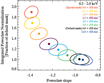
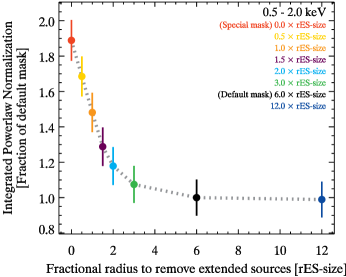
Figure 22: Best-fit parameters of the powerlaw fit of the LSS power spectrum (Section 4) for different fractional radii of the circular exclusion area of resolved extended sources. Solid ellipses and lines represent one standard deviation of a two parameter fit. The gray dotted curve on the bottom panel is just for visualization purposes. The powerlaw normalization is obtained by integrating the model over the angular scale range $10\arcsec-20\arcmin$ (Units: $\mathrm{counts^{2}\,s^{-2}\,deg^{-3}}$). See Appendix C.5 for details.

C.5 Circular exclusion area of resolved extended sources

Here, we test how the LSS power spectrum (Section 4) changes, when we gradually increase the radius of the circular exclusion area of resolved extended sources. We test eight different cases, where the radius is between $0.0$ and $12.0$ times the size of resolved extended sources (short: rES-size), which was determined by K05 (Table 1). The case of $0.0\times\text{rES-size}$ represents our special mask (Figure 2), where all resolved extended sources are retained, while $6.0\times\text{rES-size}$ represents our default mask (Figure 1). The best-fit parameters of the powerlaw fit for the LSS power spectrum are shown in Figure 22. They suggests that for our default mask, we are able to remove sufficiently well the correlation signal of resolved clusters of galaxies in comparison to the correlation signal of unresolved ones. They also suggests that the LSS power spectrum is sensitive to the structure of the clusters of galaxies, alias the surface-brightness profile of the ICM. However, proper modeling is necessary in order to substantiate this quantitatively (e.g. Paper III).

Table 2: Main characteristics of the combined, mosaic, and stacked power spectra.

Name	Angular scales	Angular frequencies	Based on
	$\theta$	$\log_{10}(k[\mathrm{arcsec^{-1}}])$
Combined power spectrum $P(k)$	$[\sim 1\arcsec,\sim 3^{\circ}]$	$[-4.0,-0.0]$	$P(k)=P_{S}[\sim 1\arcsec,k_{\mathrm{C}}]+P_{\mathrm{M}}[k_{\mathrm{C}},\sim 3^{\circ}]$
Mosaic power spectrum $P_{\mathrm{M}}(k)$	$[\sim 32\arcsec,\sim 3^{\circ}]$	$[-4.0,-1.5]$	fluctuation mosaic ($\delta\mathbb{F}$), image-pixel-binning $b=32$
Stacked power spectrum $P_{S}(k)$	$[\sim 1\arcsec,\sim 17\arcmin]$	$[-3.0,-0.0]$	fluctuation maps ($\delta\textit{{F}}$), image-pixel-binning $b=1$

The lower limit in angular scales is defined by the Nyquist-Frequency $k_{\mathrm{Ny}}=(2\,b\,\Delta p)^{-1}$, where $\Delta p$ is ACIS-I’s chip-pixel-size ($0.492\arcsec$) and $b$ is the image-pixel-binning of the fluctuation mosaic ($b=32$) or fluctuation maps ($b=1$). The upper limit in angular scales for the stacked power spectrum is defined by ACIS-I’s FOV, while the upper limit for the mosaic power spectrum is defined by the geometry of the XBOOTES survey. The combine frequency is $k_{\mathrm{C}}=k_{\mathrm{Ny}}^{\mathrm{Mosaic}}/2\approx(63\arcsec)^{-1}\approx 0.016\,\mathrm{arcsec^{-1}}$. Also see Section 3 and Appendix C.6.

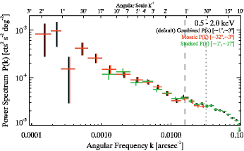
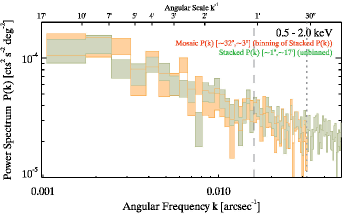
Figure 23: Comparison of the combined (black, default), mosaic (red) and stacked (green) power spectra in the $0.5-2.0\,\mathrm{keV}$ band for the default mask. Also shown are the combine frequency ($k_{\mathrm{C}}$) as gray dashed vertical line and the Nyquist frequency for the mosaic power spectrum ($k_{\mathrm{Ny}}^{\mathrm{Mosaic}}$) as gray dotted vertical line. Top: All power spectra are adaptively binned (default). Bottom: The stacked power spectrum is unbinned, while the binning of the mosaic power spectrum matches the unbinned stacked power spectrum. See Section 3 and Appendix C.6 for details.

C.6 Comparison of mosaic and stacked power spectra

In Figure 23 we directly compare the mosaic (red) and stacked (green) power spectra defined in Section 3 and summarized in Table 2. We can see that the stacked and mosaic power spectra agree rather well, although it is not a perfect match. We notice some small modulations, which can be seen as our systematic uncertainties between the stacked and mosaic power spectra. They arise mainly from the (uncorrected) mask effect, which correlates adjacent Fourier frequencies and suppresses the power spectrum on large angular scales (for the latter see Appendix C.1 for the mosaic power spectrum and appendix D.1 of Paper I for the stacked power spectrum). Since the dimensions of the masks used for the mosaic and stacked power spectra are an order of magnitude different ($\approx 3.66^{\circ}$ and $\approx 0.40^{\circ}$ side length, respectively, Section 2.2.1), the impact of the mask effect onto the power spectrum is also different for a given angular scale. To demonstrate that stacked and mosaic power spectra are essentially fluctuating around a true (i.e. mask effect corrected) power spectrum, we also show in the bottom panel of Figure 23 the unbinned stacked power spectrum in comparison to the mosaic power spectrum, which binning matches the unbinned stacked power spectrum.

We set the combine frequency ($k_{\mathrm{C}}$) to be two times smaller than the Nyquist-Frequency of the mosaic power spectrum ($k_{\mathrm{C}}=k_{\mathrm{Ny}}^{\mathrm{Mosaic}}/2\approx 0.016\,\mathrm{arcsec^{-1}}\approx(63\arcsec)^{-1}$) as a precaution in order to avoid possible systematic uncertainties in estimating the photon shot noise of the mosaic power spectrum (Appendix A), and possible numerical inaccuracies of our discrete Fourier transform (section 4.1 of Paper I), which become important very close to the Nyquist-Frequency (e.g. Jing, 2005).

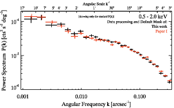
Figure 24: Comparison of the stacked power spectra in the $0.5-2.0\,\mathrm{keV}$ band for the data processing of this work (black) and of Paper I (red) for the default mask. See Section 2.1 and Appendix C.7 for details.

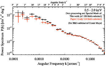
Figure 25: Comparison of the combined power spectra in the $0.5-2.0\,\mathrm{keV}$ band for the data processing of this work (black) and of Paper I (red) for the special mask. Note, that in this work all 126 observations of XBOOTES are considered, while for Paper I only 118 observations are considered (section 2 of Paper I). Also see Section 2.1.1 and Appendix C.7 for details.

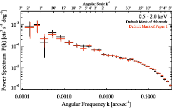
Figure 26: Comparison of the combined power spectra in the $0.5-2.0\,\mathrm{keV}$ band for the default mask of this work (black) and of Paper I (red). The removal of resolved point sources is different (see Section 2.1.4 for details), while the removal of resolved extended sources is the same. Also see Section 2.1.4 and Appendix C.7 for details.

C.7 Comparison of previous and current data processing

Figure 24 shows that the stacked power spectra for the data processing of this work (black) and of Paper I (red) have overall a good agreement with each other for the default mask, although the field selection, exposure map and the FOV mask, the used count maps, and the removal of resolved point sources have changed from Paper I to this work (Section 2.1). Note, that we rescaled the power spectrum of Paper I by the factor $(\langle E_{\mathrm{Paper~{}I}}\rangle/\langle E_{\mathrm{This~{}work}}\rangle)^{2}\approx 0.86$, to account for the different average exposure times $\langle E\rangle$ of both data processing (Section 2.2.2), which allows us a better comparison of the shape of both power spectra. Given this good agreement for the default mask, we can concluded that also with the processed data of this work we would have come to the same result of Paper I.

For the special mask the agreement is as good as for the default mask, if one keeps the field selection fixed to either the one from this work or from Paper I (Section 2.1.1). If one uses the default field selections, 118 observations for Paper I and all 126 observations for this work, there is however a significant disagreement of the corresponding power spectra on angular scales above $\gtrsim 7\arcmin$. This can be seen in Figure 25, where we show the combined power spectra to demonstrate that the field selection is also important on large angular scales above ACIS-I’s FOV ($\gtrsim 17\arcmin$) for the special mask. Note, that in Figure 25 we had to use background-subtracted count maps (C) also for the power spectra of Paper I due the issues explained in Appendix C.2. This discrepancy arises from the fact that the field selection of this work leads to a higher number of retained resolved extended sources than the field selection of Paper I, which was the main motivation to change the field selection. This also means that the conclusions drawn from the power spectrum of the special mask in Paper I (section 5) would still remain the same with the current processed data.

In this work we simplified the method of removing resolved point sources in comparison to Paper I (see Section 2.1.4 for details). Figure 26 shows that the combined power spectra of the default mask of this work (black) and of Paper I (red) agree very well with each other. This agreement illustrates that both methods give consistent results on all considered angular scales. This is reassuring because with the simplified method of this work we reduce the size of the circular exclusion area, which leads to an increase in the number of residual counts per removed point source. If such an increase in residual counts would alter the power spectrum significantly then we would expect to see the largest differences on small angular scales. Fortunately, this is not the case for the given S/N.

References

- Aird et al. (2010) Aird J. et al., 2010, MNRAS, 401, 2531
- Alexander & Hickox (2012) Alexander D. M., Hickox R. C., 2012, New A Rev., 56, 93
- Alexander et al. (2013) Alexander D. M. et al., 2013, ApJ, 773, 125
- Anders & Grevesse (1989) Anders E., Grevesse N., 1989, Geochim. Cosmochim. Acta, 53, 197
- Anderson et al. (2015) Anderson M. E., Gaspari M., White S. D. M., Wang W., Dai X., 2015, MNRAS, 449, 3806
- Arnaud (1996) Arnaud K. A., 1996, in Astronomical Society of the Pacific Conference Series, Vol. 101, Astronomical Data Analysis Software and Systems V, Jacoby G. H., Barnes J., eds., p. 17
- Barcons & Fabian (1988) Barcons X., Fabian A. C., 1988, MNRAS, 230, 189
- Brandt & Alexander (2015) Brandt W. N., Alexander D. M., 2015, A&A Rev., 23, 1
- Brandt & Hasinger (2005) Brandt W. N., Hasinger G., 2005, ARA&A, 43, 827
- Bregman (2007) Bregman J. N., 2007, ARA&A, 45, 221
- Cappelluti, Allevato & Finoguenov (2012) Cappelluti N., Allevato V., Finoguenov A., 2012, Advances in Astronomy, 2012, 1
- Cappelluti et al. (2013) Cappelluti N. et al., 2013, ApJ, 769, 68
- Cappelluti et al. (2012) Cappelluti N. et al., 2012, MNRAS, 427, 651
- Cen & Ostriker (2006) Cen R., Ostriker J. P., 2006, ApJ, 650, 560
- Davé et al. (2001) Davé R. et al., 2001, ApJ, 552, 473
- Eckert et al. (2017) Eckert D., Ettori S., Pointecouteau E., Molendi S., Paltani S., Tchernin C., 2017, Astronomische Nachrichten, 338, 293
- Eckert et al. (2015) Eckert D. et al., 2015, Nature, 528, 105
- Eckert et al. (2012) Eckert D. et al., 2012, A&A, 541, A57
- Eisenhardt et al. (2004) Eisenhardt P. R. et al., 2004, ApJS, 154, 48
- Ettori et al. (2013) Ettori S., Donnarumma A., Pointecouteau E., Reiprich T. H., Giodini S., Lovisari L., Schmidt R. W., 2013, Space Sci. Rev., 177, 119
- Galeazzi, Gupta & Ursino (2009) Galeazzi M., Gupta A., Ursino E., 2009, ApJ, 695, 1127
- Georgakakis et al. (2008) Georgakakis A., Nandra K., Laird E. S., Aird J., Trichas M., 2008, MNRAS, 388, 1205
- Giacconi et al. (1962) Giacconi R., Gursky H., Paolini F. R., Rossi B. B., 1962, Physical Review Letters, 9, 439
- Giles et al. (2016) Giles P. A. et al., 2016, A&A, 592, A3
- Gilli, Comastri & Hasinger (2007) Gilli R., Comastri A., Hasinger G., 2007, A&A, 463, 79
- Giodini et al. (2013) Giodini S., Lovisari L., Pointecouteau E., Ettori S., Reiprich T. H., Hoekstra H., 2013, Space Sci. Rev., 177, 247
- Goulding et al. (2012) Goulding A. D. et al., 2012, ApJS, 202, 6
- Hamilton & Helfand (1987) Hamilton T. T., Helfand D. J., 1987, ApJ, 318, 93
- Hasinger, Miyaji & Schmidt (2005) Hasinger G., Miyaji T., Schmidt M., 2005, A&A, 441, 417
- Heckman & Best (2014) Heckman T. M., Best P. N., 2014, ARA&A, 52, 589
- Helgason et al. (2014) Helgason K., Cappelluti N., Hasinger G., Kashlinsky A., Ricotti M., 2014, ApJ, 785, 38
- Helgason et al. (2016) Helgason K., Ricotti M., Kashlinsky A., Bromm V., 2016, MNRAS, 455, 282
- Henley & Shelton (2013) Henley D. B., Shelton R. L., 2013, ApJ, 773, 92
- Hickox et al. (2009) Hickox R. C. et al., 2009, ApJ, 696, 891
- Hickox & Markevitch (2006) Hickox R. C., Markevitch M., 2006, ApJ, 645, 95
- Hickox & Markevitch (2007) Hickox R. C., Markevitch M., 2007, ApJ, 661, L117
- Hopkins et al. (2006) Hopkins P. F., Hernquist L., Cox T. J., Di Matteo T., Robertson B., Springel V., 2006, ApJS, 163, 1
- Hütsi et al. (2014) Hütsi G., Gilfanov M., Kolodzig A., Sunyaev R., 2014, A&A, 572, A28
- Jannuzi et al. (2004) Jannuzi B. T., Dey A., Brown M. J. I., Tiede G. P., NDWFS Team, 2004, in Bulletin of the American Astronomical Society, Vol. 36, American Astronomical Society Meeting Abstracts #204, p. 745
- Jing (2005) Jing Y. P., 2005, ApJ, 620, 559
- Kaastra et al. (2013) Kaastra J. et al., 2013, ArXiv e-prints
- Kalberla et al. (2005) Kalberla P. M. W., Burton W. B., Hartmann D., Arnal E. M., Bajaja E., Morras R., Pöppel W. G. L., 2005, A&A, 440, 775
- Kenter et al. (2005) Kenter A. et al., 2005, ApJS, 161, 9
- Kim et al. (2007) Kim M., Wilkes B. J., Kim D.-W., Green P. J., Barkhouse W. A., Lee M. G., Silverman J. D., Tananbaum H. D., 2007, ApJ, 659, 29
- Kolodzig et al. (2013a) Kolodzig A., Gilfanov M., Hütsi G., Sunyaev R., 2013a, A&A, 558, A90
- Kolodzig et al. (2017) Kolodzig A., Gilfanov M., Hütsi G., Sunyaev R., 2017, MNRAS, 466, 3035
- Kolodzig et al. (2013b) Kolodzig A., Gilfanov M., Sunyaev R., Sazonov S., Brusa M., 2013b, A&A, 558, A89
- Komatsu & Seljak (2001) Komatsu E., Seljak U., 2001, MNRAS, 327, 1353
- Kravtsov & Borgani (2012) Kravtsov A. V., Borgani S., 2012, ARA&A, 50, 353
- Krumpe, Miyaji & Coil (2014) Krumpe M., Miyaji T., Coil A. L., 2014, in Multifrequency Behaviour of High Energy Cosmic Sources, pp. 71–78
- Lehmer et al. (2012) Lehmer B. D. et al., 2012, ApJ, 752, 46
- Lieu et al. (2016) Lieu M. et al., 2016, A&A, 592, A4
- Lumb et al. (2002) Lumb D. H., Warwick R. S., Page M., De Luca A., 2002, A&A, 389, 93
- Luo et al. (2017) Luo B. et al., 2017, ApJS, 228, 2
- Markwardt (2009) Markwardt C. B., 2009, in Astronomical Society of the Pacific Conference Series, Vol. 411, Astronomical Data Analysis Software and Systems XVIII, Bohlender D. A., Durand D., Dowler P., eds., p. 251
- Merloni et al. (2012) Merloni A. et al., 2012, ArXiv e-prints, 1209.3114
- Mitchell-Wynne et al. (2016) Mitchell-Wynne K., Cooray A., Xue Y., Luo B., Brandt W., Koekemoer A., 2016, ApJ, 832, 104
- Miyaji & Griffiths (2002) Miyaji T., Griffiths R. E., 2002, ApJ, 564, L5
- Miyaji et al. (2015) Miyaji T. et al., 2015, ApJ, 804, 104
- Murray et al. (2005) Murray S. S. et al., 2005, ApJS, 161, 1
- Nevalainen et al. (2015) Nevalainen J. et al., 2015, A&A, 583, A142
- Pacaud et al. (2016) Pacaud F. et al., 2016, A&A, 592, A2
- Pierre et al. (2016) Pierre M. et al., 2016, A&A, 592, A1
- Predehl et al. (2010) Predehl P. et al., 2010, in Society of Photo-Optical Instrumentation Engineers (SPIE) Conference Series, Vol. 7732, Society of Photo-Optical Instrumentation Engineers (SPIE) Conference Series
- Revnivtsev, Gilfanov & Churazov (1999) Revnivtsev M., Gilfanov M., Churazov E., 1999, A&A, 347, L23
- Reynolds et al. (2014) Reynolds M. T., Reis R. C., Miller J. M., Cackett E. M., Degenaar N., 2014, MNRAS, 441, 3656
- Roncarelli et al. (2012) Roncarelli M., Cappelluti N., Borgani S., Branchini E., Moscardini L., 2012, MNRAS, 424, 1012
- Roncarelli et al. (2006) Roncarelli M., Moscardini L., Tozzi P., Borgani S., Cheng L. M., Diaferio A., Dolag K., Murante G., 2006, MNRAS, 368, 74
- Rosati, Borgani & Norman (2002) Rosati P., Borgani S., Norman C., 2002, ARA&A, 40, 539
- Scheuer (1974) Scheuer P. A. G., 1974, MNRAS, 166, 329
- Shafer & Fabian (1983) Shafer R. A., Fabian A. C., 1983, in IAU Symposium, Vol. 104, Early Evolution of the Universe and its Present Structure, Abell G. O., Chincarini G., eds., pp. 333–342
- Soltan & Hasinger (1994) Soltan A., Hasinger G., 1994, A&A, 288, 77
- Sun et al. (2009) Sun M., Voit G. M., Donahue M., Jones C., Forman W., Vikhlinin A., 2009, ApJ, 693, 1142
- Szabo et al. (2011) Szabo T., Pierpaoli E., Dong F., Pipino A., Gunn J., 2011, ApJ, 736, 21
- Tempel et al. (2014) Tempel E., Stoica R. S., Martínez V. J., Liivamägi L. J., Castellan G., Saar E., 2014, MNRAS, 438, 3465
- Tempel et al. (2017) Tempel E., Tuvikene T., Kipper R., Libeskind N. I., 2017, A&A, 602, A100
- Ueda et al. (2014) Ueda Y., Akiyama M., Hasinger G., Miyaji T., Watson M. G., 2014, ApJ, 786, 104
- Ursino et al. (2011) Ursino E., Branchini E., Galeazzi M., Marulli F., Moscardini L., Piro L., Roncarelli M., Takei Y., 2011, MNRAS, 414, 2970
- Ursino, Galeazzi & Huffenberger (2014) Ursino E., Galeazzi M., Huffenberger K., 2014, ApJ, 789, 55
- Vajgel et al. (2014) Vajgel B., Jones C., Lopes P. A. A., Forman W. R., Murray S. S., Goulding A., Andrade-Santos F., 2014, ApJ, 794, 88
- Vikhlinin & Forman (1995) Vikhlinin A., Forman W., 1995, ApJ, 455, L109
- Vikhlinin et al. (2006) Vikhlinin A., Kravtsov A., Forman W., Jones C., Markevitch M., Murray S. S., Van Speybroeck L., 2006, ApJ, 640, 691
- Werner et al. (2008) Werner N., Finoguenov A., Kaastra J. S., Simionescu A., Dietrich J. P., Vink J., Böhringer H., 2008, A&A, 482, L29
- Xue et al. (2011) Xue Y. Q. et al., 2011, ApJS, 195, 10
- Yang et al. (2015) Yang Q.-X., Xie F.-G., Yuan F., Zdziarski A. A., Gierliński M., Ho L. C., Yu Z., 2015, MNRAS, 447, 1692
- Yue, Ferrara & Helgason (2016) Yue B., Ferrara A., Helgason K., 2016, MNRAS, 458, 4008
- Yue et al. (2013) Yue B., Ferrara A., Salvaterra R., Xu Y., Chen X., 2013, MNRAS, 433, 1556