Dynamical properties of heterogeneous nucleation of parallel hard squares

Abstract

We use the Dynamic Density-Functional Formalism and the Fundamental Measure Theory as applied to a fluid of parallel hard squares to study the dynamics of heterogeneous growth of non-uniform phases with columnar and crystalline symmetries. The hard squares are (i) confined between soft repulsive walls with square symmetry, or (ii) exposed to external potentials that mimic the presence of obstacles with circular, square, rectangular or triangular symmetries. For the first case the final equilibrium profile of a well commensurated cavity consists of a crystal phase with highly localized particles in concentric square layers at the nodes of a slightly deformed square lattice. We characterize the growth dynamics of the crystal phase by quantifying the interlayer and intralayer fluxes and the non-monotonicity of the former, the saturation time, and other dynamical quantities. The interlayer fluxes are much more monotonic in time, and dominant for poorly commensurated cavities, while the opposite is true for well commensurated cells: although smaller, the time evolution of interlayer fluxes are much more complex, presenting strongly damped oscillations which dramatically increase the saturation time. We also study how the geometry of the obstacle affects the symmetry of the final equilibrium non-uniform phase (columnar vs. crystal). For obstacles with fourfold symmetry, (circular and square) the crystal is more stable, while the columnar phase is stabilized for obstacles without this symmetry (rectangular or triangular). We find that, in general, density waves of columnar symmetry grow from the obstacle. However, additional particle localization along the wavefronts gives rise to a crystalline structure which is conserved for circular and square obstacles, but destroyed for the other two obstacles where columnar symmetry is restored.

I Introduction

The Dynamic Density Functional Theory (DDFT) has proved, since its first derivation in Ref. umberto1 , to be a very useful tool to extend the study of soft matter systems from equilibrium to non-equilibrium situations. The response of colloidal systems to time dependent, in general inhomogeneous, external fields has been extensively studied within this formalism Tarazona1 ; Tarazona3 ; lowen7 ; lowen8 . The diffusion of vacancies through a crystalline structure Teeffelen , the heterogeneous crystal nucleation lowen4 ; lowen6 , the dynamics of sedimentation processes Schmidt8 ; umberto3 , the diffusion of colloidal spheres Roth1 or rods in nematics and smectics Dijkstra ; Grelet , and the study of confined self-propelled rods lowen5 , are important examples of the variety of systems that were extensively studied within this theoretical tool. The orientational degrees of freedom of rods generate an additional complication in the numerical implementation of DDFT, which can be avoided by resorting to the restricted-orientation (Zwanzig) approximation Oettel . We should bear in mind that this formalism was derived from the stochastic Langevin dynamics of Brownian particles in the overdamped limit umberto1 , and some caution should be taken to use it in far-from-equilibrium situations. In general, the relaxation to the equilibrium dynamics is reasonably well described by DDFT.

By construction, better performance of DDFT is obtained when the system at equilibrium is well described by an approximate grand-canonical free-energy density functional (DF), the main ingredient of DDFT. Recent work has extended the DDFT by using a canonical DF (extracted from the grand-canonical one), which is more appropriate for systems with fixed number of particles Heras . As is well known, the DFs with the highest performance are those for hard particle interactions, such as hard rods in 1D Percus (whose DF is known exactly), parallel hard squares (PHS) Cuesta1 ; Cuesta2 or hard disks (HD) disks in 2D, and hard spheres (HS) Roth2 in 3D, all of them based on the original FMT proposed by Rosenfeld Rosenfeld1 . Some coarse-grained DFs, such as those based on phase-field-crystal models, are obtained from microscopic DFs by an appropriate order-parameter gradient expansion. These models were successfully used to study the dynamical properties of heterogeneous crystallization in monolayers of paramagnetic colloidal spheres lowen2 . The phase-field-crystal approximation was also used to explore, through its numerically tractable implementation, all possible stable two- and three-dimensional liquid-crystal textures as a function of some parameters lowen2 describing particle interactions. There exist recent works on DDFT studies of fluids of HD and HS using accurate DFs Roth1 ; confined . However these studies are scarce due to their complicated numerical implementation; in contrast, phase-field approximations are simpler due to the local dependence of the free-energy on the order parameters.

The purpose of the present study is twofold. (i) We use an accurate DF, based on Fundamental-Measure Theory (FMT), in combination with DDFT, to study the relaxation dynamics in fluids of PHS. The DF model used Cuesta1 ; Cuesta2 has been tested at bulk and in highly confined situations miguel2 . Our study extends the type of particle geometries (HD and HS) considered thus far. (ii) As shown below in this section, the FMT for PHS predicts the stability of columnar (C) and crystal (K) phases for particular density intervals. The present model may be used to understand how the dynamical properties of heterogeneous nucleation induced by external potentials depend on the degree of commensuration between the C or K lattice parameters and the characteristic lengths of the confining external potentials. We are interested in the full dynamics, from the initial to the final equilibrium states. For some external potentials and thermodynamic conditions, the system can be dynamically arrested in metastable states for very long times. We characterize the dynamics of confined PHS inside square cavities in terms of relaxation times and of properties of the interlayer and intralayer fluxes such as non-monotonicity, maximum values, etc. The heterogeneous nucleation of C and K phases from obstacles with different geometries are also studied. The symmetry of the growing phase crucially depends on the geometry and size of obstacles, and in fact for carefully selected obstacles an unstable phase at bulk can nucleate.

The FMT theory applied to a fluid of PHS predicts the equation of state (EOS) shown in Fig. 1. The fluid (F) phase is stable up to a mean packing fraction $\eta_{0}=\rho_{0}\sigma^{2}$ ($\sigma$ is the side length of the squares) equal to 0.534, at which a second-order transition to a columnar (C) phase takes place. The latter is stable up to $\eta_{0}\simeq 0.73$ (from free DF minimization roij ) or $\eta_{0}\simeq 0.75$ (from a Gaussian density-profile parameterization miguel2 ). For higher densities a crystalline phase (K) with simple square symmetry is stable up to close packing. See Fig. 2 for a sketch of the different stable phases.

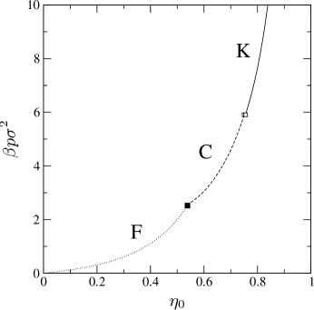
Figure 1: Equation of state (pressure in reduced units vs. mean packing fraction) of PHS from FMT.

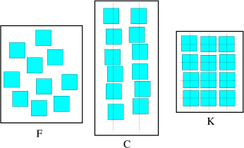
Figure 2: (Color online). Sketch of F, C and K phases (from left to right) that the FMT of PHS predicts.

The article is organized as follows. In Sec. II we present the model and the FMT-based DF which is used to implement DDFT. We specify in Sec. II.1 the external potential and the initial conditions used to study crystallization induced by confinement, while in Sec. II.2 we define the quantities that characterize the dynamics. In Sec. III results for the crystallization of PHS induced by confinement are presented. This section is in turn divided into three parts devoted to different initial conditions used: uniform (Sec. III.1), C (Sec. III.2) and K (Sec. III.3) density profiles as initial conditions. Sec. IV is concerned with the study of heterogeneous nucleation of C and K phases induced by the presence of obstacles of different sizes and symmetries. Finally some conclusions are drawn in Sec. V.

II Model

The relaxation dynamics to equilibrium is studied using the DDFT formalism of Ref. umberto1 ,

$$\frac{\partial\rho}{\partial t}({\bm{r}},t)=-\bm{\nabla}\cdot{\bm{J}}({\bm{r}},t),$$ (1)

where $\rho({\bm{r}},t)$ is the local density. The local flux, ${\bm{J}}({\bm{r}},t)$, is defined by

$${\bm{J}}({\bm{r}},t)=-{\cal D}\rho({\bm{r}},t)\bm{\nabla}\frac{\delta\beta{\cal F}[\rho]}{\delta\rho({\bm{r}},t)},$$ (2)

where ${\cal D}$ is the diffusion constant, and

$$\beta{\cal F}[\rho]=\int d{\bm{r}}\left[\Phi({\bm{r}},t)+\rho({\bm{r}},t)\beta V_{\rm ext}({\bm{r}},t)\right],$$ (3)

is the free-energy DF. $\beta=1/k_{B}T$ is the inverse temperature, $V_{\rm ext}({\bm{r}},t)$ is the confining external potential, and $\Phi({\bm{r}},t)=\Phi_{\rm id}({\bm{r}},t)+\Phi_{\rm ex}({\bm{r}},t)$ is the free-energy density, which is split in ideal

$$\Phi_{\rm id}({\bm{r}},t)=\rho({\bm{r}},t)\left\{\log{\left[\rho({\bm{r}},t)\Lambda^{2}\right]}-1\right\},$$ (4)

and excess

$$\Phi_{\rm ex}({\bm{r}},t)=-n_{0}({\bm{r}},t)\log\left[1-n_{2}({\bm{r}},t)\right]+\frac{n_{1x}({\bm{r}},t)n_{1y}({\bm{r}},t)}{1-n_{2}({\bm{r}},t)},$$

parts. $\Lambda$ is the thermal length. The excess part corresponds to PHS Cuesta1 ; Cuesta2 , and the weighted densities $n_{\alpha}({\bm{r}},t)=\int d{\bm{r}}^{\prime}\rho({\bm{r}}^{\prime},t)\omega^{(\alpha)}({\bm{r}}-{\bm{r}}^{\prime})$, are convolutions of the density profile and the following one-particle weighting functions:

$$\omega^{(0)}({\bm{r}})=\frac{1}{4}\delta\left(\frac{\sigma}{2}-|x|\right)\delta\left(\frac{\sigma}{2}-|y|\right),$$ (6)

$$\omega^{(1x)}({\bm{r}})=\frac{1}{2}\Theta\left(\frac{\sigma}{2}-|x|\right)\delta\left(\frac{\sigma}{2}-|y|\right),$$ (7)

$$\omega^{(1y)}({\bm{r}})=\frac{1}{2}\delta\left(\frac{\sigma}{2}-|x|\right)\Theta\left(\frac{\sigma}{2}-|y|\right),$$ (8)

$$\omega^{(2)}({\bm{r}})=\Theta\left(\frac{\sigma}{2}-|x|\right)\Theta\left(\frac{\sigma}{2}-|y|\right).$$ (9)

$\delta(x)$ and $\Theta(x)$ are the Dirac-delta and Heaviside functions, respectively.

II.1 External potential and initial conditions

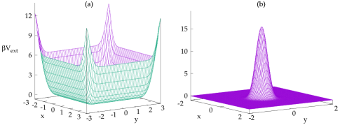
Figure 3: (Color online). Form of the external potentials defined by Eqs. (10) (a) and (12) (b).

Our first study concerns the dynamic evolution to equilibrium of a fluid of confined PHS when the confining external potential is switched on at $t=0$. The potential is defined in a region $x\in[-\frac{h}{2},\frac{h}{2}]$, $y\in[-\frac{h}{2},\frac{h}{2}]$, where $h$ is the side of the square cavity. The following form is used:

$$\beta V_{\rm ext}({\bm{r}},t)=-\epsilon\log\left\{\left[1-\Psi(x)\right]\times\left[1-\Psi(y)\right]\right\}\Theta(t),$$ (10)

where

$$\Psi(z-h/2)=\frac{1}{2}\sum_{k=-N}^{N}\left\{\text{erf}\left[\sqrt{\alpha}\left(z+\frac{\sigma}{2}+kh\right)\right]\right.$$

$$\left.-\text{erf}\left[\sqrt{\alpha}\left(z-\frac{\sigma}{2}+kh\right)\right]\right\},\quad z=\{x,y\},$$ (11)

with erf$(x)$ the standard error function. The external potential acts on the particles as a quickly decaying soft wall with characteristic inverse square length $\alpha$ and an amplitude $\epsilon$ that defines the height of the barrier. For the sake of computational convenience, the box is periodically replicated, as defined by the sum over $k$ in Eqn. (11), forming a square lattice of boxes. The number of boxes, dictated by the value of $N$, is chosen large enough to guarantee the convergence of the sum (11) for $(x,y)\in[-\frac{h}{2},\frac{h}{2}]\times[-\frac{h}{2},\frac{h}{2}]$. In Fig. 3(a) the function $\beta V_{\rm ext}({\bm{r}},0)$ is plotted for some particular values of the parameters $\epsilon$, $\alpha$ and $h$.

In a second study we analyse the heterogeneous nucleation around obstacles with different geometries. For a circular obstacle, we define a repulsive external potential centred at ${\bm{r}}={\bm{0}}$:

$$\beta V_{\rm ext}({\bf r},t)=\epsilon\log\left[1+\Psi\left(\sqrt{x^{2}+y^{2}}\right)\right]\Theta(t),$$ (12)

where

$$\Psi(z)=\frac{1}{2}\left\{\text{erf}\left[\sqrt{\alpha}\left(z+D\right)\right]-\text{erf}\left[\sqrt{\alpha}\left(z-D\right)\right]\right\}.$$

Here $\epsilon$ and $\alpha$ have the same meaning as before, while $D$ is the characteristic dimension of the obstacle, in this case its diameter. In Fig. 3 (b) we plot the external potential for $D=1$ and certain values of the parameters $\{\epsilon,\alpha\}$. For a rectangular obstacle we use

$$\beta V_{\rm ext}({\bf r},t)=\epsilon\log\left[1+\Psi_{x}\left(x)\Psi_{y}(y)\right)\right]\Theta(t),$$ (14)

where

$$\Psi_{k}(z)=\frac{1}{2}\left\{\text{erf}\left[\sqrt{\alpha}\left(z+D_{k}\right)\right]-\text{erf}\left[\sqrt{\alpha}\left(z-D_{k}\right)\right]\right\}.$$

$D_{x}$ and $D_{y}$ are the side-lengths of the rectangular obstacle along $x$ and $y$, respectively. The long, $L=D_{y}$, and short, $D=D_{x}$, lengths of the rectangle will always be chosen to be parallel to the $y$ and $x$ axes, respectively. For $D_{x}=D_{y}=D$ we are describing a square obstacle.

It can be shown easily that the dynamic evolution that follows from Eqns. (1) and (2) conserve the total number of particles, $N=\int_{A_{\rm cell}}d{\bm{r}}\rho({\bm{r}},t)$, where $A_{\rm cell}=[-\frac{h}{2},\frac{h}{2}]\times[-\frac{h}{2},\frac{h}{2}]$ is the area of the unit cell defined by the external potential. Three different initial conditions were used for the density profiles: (i) $\rho({\bm{r}},0)=\rho_{0}$, i.e. a uniform density profile, (ii) $\rho({\bm{r}},0)=\rho_{0}^{(\rm C)}(y)$, corresponding to the bulk equilibrium density profile of columnar (C) symmetry, and (iii) $\rho({\bm{r}},0)=\rho_{0}^{(\rm K)}({\bm{r}})$, corresponding to the scaled bulk equilibrium density profile of crystalline (K) symmetry. Both density profiles were previously calculated by fixing the mean number density $\rho_{0}$ (obtained from integration of the density profile over the unit cell) to those values for which these phases are stable or metastable at bulk. By scaled density profile we mean an equilibrium density profile scaled along the $x$ and $y$ directions so as to commensurate with the unit cell of the external potential, multiplied by a corresponding factor to obtain the same mean number density $\rho_{0}=A_{\rm cell}^{-1}\int_{A_{\rm cell}}d{\bm{r}}\rho({\bm{r}},0)$.

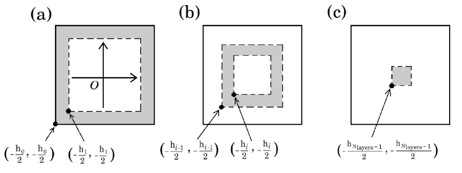
Figure 4: Schematic of the square rings defined. (a) First layer. (b) Intermediate layer. (c) Central layer.

II.2 Quantities to characterize the dynamics

In this section we define the different quantities that characterize the relaxation dynamics. As shown in Sec. III the final equilibrium state of the confined system consists of well-localized density peaks positioned in concentric square-like chains. We define a layer $A_{i}$ ($i=1,\dots,{\cal N}_{\rm layers}$) as a square ring containing each of the above chains and with boundaries defined by joining the local minima of $\rho_{\rm eq}({\bm{r}})$ between neighbor chains. The minima are located on the lines defined by

$$\left(\pm\frac{h_{j}}{2},y\right),\hskip 11.38092pt-\frac{h_{j}}{2}\leq y\leq\frac{h_{j}}{2},$$

$$\left(x,\pm\frac{h_{j}}{2}\right),\hskip 11.38092pt-\frac{h_{j}}{2}\leq x\leq\frac{h_{j}}{2},$$ (16)

where $j=0,\cdots,{\cal N}$ (with ${\cal N}=N_{\rm layers}$ for $N_{\rm layers}$ even, and ${\cal N}=N_{\rm layers}-1$ for $N_{\rm layers}$ odd), while $h_{0}=h$ and $h_{{\cal N}_{\rm layers}}=0$. The first layer is located next to the soft walls, while the last layer is at the centre. The $i$th layer is then defined by the region (see Fig. 4)

$$\frac{h_{i}}{2}\leq\left|x\right|\leq\frac{h_{i-1}}{2},\hskip 17.07182pt\frac{h_{i}}{2}\leq\left|y\right|\leq\frac{h_{i-1}}{2}.$$ (17)

The innermost chain consists of either a single particle or four particles, depending on whether the total number of layers is an odd or an even number, respectively.

The total particle flux across the boundaries of $A_{i}$ (the interlayer flux) is in turn equal to minus the exchange rate in number of particles, $-N_{i}^{\prime}(t)$, inside $A_{i}$, as can be shown by integrating Eq. (1) over $A_{i}$:

$${\cal J}_{i}^{(\rm inter)}(t)\equiv-N_{i}^{\prime}(t)=-\frac{d}{dt}\int_{A_{i}}d{\bm{r}}\rho({\bf r},t)$$

$$=\int_{A_{i}}d{\bm{r}}\bm{\nabla}\cdot{\bm{J}}({\bm{r}},t)=\int_{{\cal L}_{i}}dl{\bm{J}}({\bm{r}},t)\cdot{\bm{n}}_{i}.$$ (18)

The last term in (18), obtained from Gauss theorem, is a line integral over the boundary ${\cal L}_{i}$ of the $i$th layer with outer normal ${\bm{n}}_{i}$. Note that the total number of particles is a conserved quantity, so that $\displaystyle\sum_{i}{\cal J}_{i}^{(\rm inter)}=0$. Using the square symmetry, it is easy to show that the line integral can be computed as

$$N_{i}^{\prime}(t)=8\left[\int_{0}^{h_{i}/2}dyJ_{x}\left(\frac{h_{i}}{2},y\right)\right.$$

$$\left.-\int_{0}^{h_{i-1}/2}dyJ_{x}\left(\frac{h_{i-1}}{2},y\right)\right],$$

where we have defined

$$J_{x}(a,y)=-\left.\rho(x,y)\frac{\partial}{\partial x}\left(\frac{\delta\beta{\cal F}[\rho]}{\delta\rho(x,y)}\right)\right|_{x=a}.$$ (20)

We define the saturation time as a time $T_{\rm sat}$ such that

$$T_{\rm sat}=t:\ \sum_{i}\left|{\cal J}^{(\rm inter)}_{i}(t)\right|<\delta,$$ (21)

where $\delta$ is a tolerance (to be defined below). The total interlayer flux over the whole cell $A_{\rm cell}=\cup_{i}A_{i}$ and integrated over time is defined as

$${\cal J}^{(\rm inter)}=\sqrt{\frac{1}{\tau_{B}}\sum_{i}\int_{0}^{T_{\rm sat}}dt\left[N_{i}^{\prime}(t)\right]^{2}},$$ (22)

where $\tau_{B}=\sigma^{2}/{\cal D}$ is the Brownian time, while the maximum value of the interlayer fluxes over the whole cell and time is quantified through

$${\cal M}^{(\rm inter)}=\text{max}_{i,t}\left(|N_{i}^{\prime}(t)|\right).$$ (23)

The non-monotonicity of the interlayer fluxes is taken into account by counting the total number of extrema of $\{N_{i}^{\prime}(t)\}$ as a function of time:

$${\cal E}^{(\rm inter)}=\sum_{i}\#\text{extrema}\left[N_{i}^{\prime}(t)\right],$$ (24)

Another useful quantity, measuring the total flux in the cell during the complete time evolution, is

$${\cal J}^{(\rm total)}=\frac{1}{\tau_{B}\sigma}\int_{0}^{T_{\rm sat}}dt\int_{A_{\rm cell}}d{\bm{r}}\left[\left|J_{x}({\bm{r}},t)\right|+\left|J_{y}({\bm{r}},t)\right|\right],$$

with $J_{x,y}({\bm{r}},t)$ the $x$ and $y$ components of ${\bm{J}}({\bm{r}},t)$.

To characterize the equilibrium density profiles we use apart from the total number of layers, ${\cal N}_{\rm layers}$, the value of the highest density peak over the whole cell:

$$\rho_{\rm max}=\text{max}_{{\bm{r}}\in A_{\rm cell}}\left[\rho_{\rm eq}({\bm{r}})\right].$$ (26)

Finally we define the mean packing fraction of the layer $i$ as

$$\eta_{i}(t)=A_{i}^{-1}\int_{A_{i}}d{\bm{r}}\rho({\bm{r}},t)\sigma^{2},$$ (27)

Note that, as the areas $A_{i}$ ($i=1,\dots,{\cal N}_{\rm layers}$) are in general different, we have that

$$\frac{1}{\cal N}_{\rm layers}\sum_{i=1}^{{\cal N}_{\rm layers}}\eta_{i}(t)$$

$$\neq\eta_{0}\equiv A_{\rm cell}^{-1}\int_{A_{\rm cell}}d{\bm{r}}\rho({\bm{r}},t)\sigma^{2}=\rho_{0}\sigma^{2},$$ (28)

i.e. the average of the mean packing fractions per layer is not a conserved quantity and it is different from the total mean packing fraction $\eta_{0}$, which is conserved.

III Crystallization induced by confinement

This section is devoted to the study of the dynamical relaxation of the confined fluid to equilibrium from different initial conditions. In Sec. III.1 we present the results obtained from constant-density initial conditions, while in Secs. III.2 and III.3 initial conditions with C and K symmetries are respectively chosen.

First we discuss an important issue on the terminology used in the article to describe the dynamic evolution of the density profile. We use sentences like "particles are expelled from the walls" or "particles are highly localized/delocalized". With this we mean that the structure of the density profile is strongly changing with time: density peaks get smeared out or sharpened in space. One should always bear in mind that there is no direct relation between a single density peak and a real particle, since density profiles measure the probability density of finding a particle at some particular position. The spatial integral of the density profile over a region with the same particle dimensions gives the probability to find the particle at this position and obviously this can be less than one even for the K phase due to the existence of vacancies. We decided to keep this terminology for simplicity, avoiding the use of an excessively elaborate language.

III.1 Dynamic evolution from a constant density profile

We use a simple iteration scheme to solve Eqn. (1): the density profile at the $n$th timestep $t_{n}=n\Delta t$ is calculated from the previous one as

$$\rho^{*}(x_{i},y_{j},n+1)=\rho^{*}(x_{i},y_{j},n)$$

$$+ \Delta\tau\bm{\nabla}\cdot\left(\rho^{*}(x_{i},y_{j},n)\bm{\nabla}\left.\frac{\delta\beta{\cal F}[\rho]}{\delta\rho}\right|_{x_{i},y_{j},n}\right),$$ (29)

$$\{i,j\}=[0,M],\ n\geq 0$$

where $\Delta\tau=\Delta t/\tau_{B}$ and $\Delta t$ is the timestep. Also $\rho^{*}=\rho\sigma^{2}$, and the variables $\{x_{i},y_{j}\}$ are the $x$ and $y$ coordinates of a node on the square grid used to discretize the cell, $[-\frac{h}{2},\frac{h}{2}]\times[-\frac{h}{2},\frac{h}{2}]$ ($M\Delta x=h$, with $\Delta x=\Delta y=\sigma/40$ the size of the spatial grid). The spatial derivatives in (29) were calculated using a central finite-difference method. As a first study, we have chosen the initial local packing fraction $\rho(x_{i},y_{j},0)\sigma^{2}=\eta_{0}=0.6$ $\forall\ \{i,j\}$, i.e. the initial density profile inside the cell is constant (and different from the bulk value, as can be seen from Fig. 1 which shows a stable C phase at $\eta_{0}=0.6$). Fig. 5 presents the equilibrium density profiles after convergence of Eqn. (29) at $T_{\rm sat}=n_{\rm sat}\Delta t$ for cells of dimensions (a) $h/\sigma=5.1$ and (b) $h/\sigma=5.8$, respectively. The value of $\delta$ used to define convergence was $\delta\cdot\tau_{B}=10^{-5}$.

Despite the fact that the C phase is stable at bulk, the confining external potential localizes particles at the nodes of a simple square lattice. The lattice parameter $a$ and the cell dimension $h$ are approximately related by $h\simeq 2{\cal N}_{\rm layers}a$ or $h\simeq\left(2{\cal N}_{\rm layers}-1\right)a$ when the number of layers, $N_{\rm layers}$, is an even or an odd integer, respectively. For the latter case case a central peak is always found at the centre of the cell. For $h/\sigma=5.8$ the density peaks are sharper and more localized than those corresponding to $h/\sigma=5.1$, which are smeared out over space. This is a consequence of the difference between the lattice parameters of the confined system, $a$, and that of the metastable K phase at bulk, $a_{\rm K}$. The C phase is stable for packing fractions in the interval $\eta_{0}\in[0.534,0.73]$. However, a metastable free-energy branch of K phase also bifurcates from the F branch at $\eta_{0}=0.534$, its free energy being above the C branch until they cross at $\eta_{0}\simeq 0.73$. When $a/a_{\rm K}\sim 1$ highly localized peaks are present in the cavity, as shown in Fig. 5 (b); otherwise the density profile is similar to that of panel (a). When commensuration between $a$ and $a_{\rm K}$ is nearly perfect [as in (b)], the density profile develops bridges between neighbor particles belonging to the same layer (with boundaries indicated by green lines). This means that particle fluctuations along these directions are so favoured that the K phase can support a large fraction of vacancies.

Fig. 6 shows the dynamic evolution of the mean packing fraction of layer $i$, $\eta_{i}(t)$, as a function of scaled time $t^{*}=t/\tau_{B}=n\Delta\tau$ for the two cells shown in Fig. 5, which contain two ($h/\sigma=5.1$) and three ($h/\sigma=5.8$) layers, respectively. For the former, the first stages of the dynamic evolution of $\eta_{1}(t)$ present a small decrease, then a minimum and an increase to its stationary value $\eta_{1}(\infty)<0.6$, which is reached at $T_{\rm sat}^{*}\equiv T_{\rm sat}/\tau_{B}\simeq 500$. In this case the repulsive potential expels the excess of particles in contact with the soft wall, creating a first layer with lower mean packing fraction. By contrast the inner layer, formed at the end by four particles, increases its packing fraction, reaches a maximum, and tends to its stationary value $\eta_{2}(\infty)>0.6$. We can see that the dynamic evolution of the case $h/\sigma=5.8$ has the opposite behavior: the packing fraction of the first layer increases rapidly, reaches a maximum, and finally decreases to a value $\eta_{1}(\infty)<0.6$, while the second layer exhibits the opposite evolution. Finally the third layer, enclosing at the end a single particle, exhibits the deepest minimum and a final relaxation to $\eta_{3}(\infty)<0.6$. As we will promptly see, cells that commensurate with the bulk lattice parameter, which exhibit highly localized equilibrium density peaks [(b)], have intralayer fluxes which dominate over the interlayer ones, while the opposite occurs when peaks are spatially smeared out, as in (a). Therefore the dominant effect of the external potential on the layers in (b) involves the motion of particles inside each layer to their equilibrium highly localized positions and, in addition, the flow of particles to or from the neighbour layers to make a regular square lattice. As a consequence of this complex dynamics, the saturation time is usually longer [$T_{\rm sat}^{*}\simeq 3000$ in (b), as compared with $500$ in (a)]. In contrast, for poorly commensurate cells [as in (a)], which give delocalized peaks, interlayer fluxes are more important and the dominant effect of the external potential on the first layer is to expel the excess of particles to the interior of the cell. The other layers get restructured by particle interchange with neighbour layers. The usual behavior in $\eta_{2}(t)$ is always opposite to that of $\eta_{1}(t)$ [see (a) and (b)]. Finally the third layer in (b), which contains a single particle, reaches an equilibrium packing fraction less than $\eta_{0}$. Although these trends are generally true, there are exceptions to these behaviours, which can be explained by the inhomogeneities of the lattice parameter $a$ from the wall to the interior of the cell.

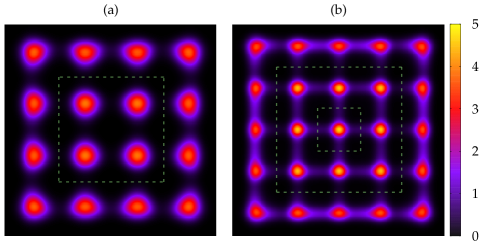
Figure 5: (Color online). Equilibrium density profiles $\rho_{\rm eq}^{*}({\bf r})$ inside the square cells of dimensions $h/\sigma=5.1$ (a) and 5.8 (b) starting from constant density profiles corresponding to packing fraction $\eta_{0}=0.6$. They are shown through false color contour plot images with colour scales correspondingly shown. Green dashed lines represent the boundaries between different layers [with a total amount of two (a) and three (b) layers].

Figure 6: Mean packing fraction of layer $i$, $\eta_{i}(t)$, as a function of time, for square cells of dimensions $h/\sigma=5.1$ (a) and 5.8 (b). With solid, dashed and dotted lines are shown $\eta_{1}(t)$, $\eta_{2}(t)$ and $\eta_{3}(t)$ respectively. The initial condition corresponds to a constant density profile with $\eta_{0}=0.6$.

Figure 7: Interlayer fluxes, ${\cal J}^{(\rm inter)}_{i}(t)$, as a function of time, for square cells of dimensions $h/\sigma=5.1$ (a) and 5.8 (b). With solid, dashed and dotted lines are shown ${\cal J}^{\rm(inter)}_{1}(t)$, ${\cal J}^{\rm(inter)}_{2}(t)$ and ${\cal J}^{\rm(inter)}_{3}(t)$ respectively. The initial condition corresponds to a constant density profile with $\eta_{0}=0.6$.

The behaviour of the interlayer fluxes ${\cal J}_{i}^{(\rm inter)}(t)$ as a function of time confirms the preceding discussion. These are shown in Fig. 7 for the same cells and initial conditions. For $h/\sigma=5.1$ the first cell becomes a source of particles, creating a positive flux across its boundaries. This flux reaches a maximum, then decays and reaches a minimum, and finally relaxes monotonically to the stationary state. Obviously the flux that crosses the boundaries of the second layer, ${\cal J}_{2}^{(\rm inter)}(t)$, is, by conservation of particles ($\displaystyle\sum_{i}{\cal J}_{i}^{(\rm inter)}=0$), the specular reflection of ${\cal J}_{1}^{(\rm inter)}(t)$ in the entire $t$-axis. The behaviour of the fluxes for $h/\sigma=5.8$ and $t^{*}>t_{c}\simeq 20$ is opposite to the previous case: particles enter the first layer from the neighbor layer, so that ${\cal J}_{1}^{(\rm inter)}(t)$ becomes a negative, decreasing function down to a minimum, and then increases, changes sign at a certain time (the layer becoming a source of particles), reaches a maximum and finally relaxes to zero at a time $T_{\rm sat}$ much longer than in the previous case. The third, innermost layer, has a positive flux which relaxes to zero after reaching a small minimum, therefore becoming a source of particles. The above behavior pertains to times $t^{*}>t_{c}$. At very short times ($t^{*}<t_{c}$) the behavior is the opposite for the first two layers, and the same for the third (see inset). This latter fact confirms a scenario where the effect of the external potential propagates from the walls to the inner layers with a finite velocity. Although the extrema of the fluxes for $t^{*}<t_{c}$ and $t^{*}>t_{c}$ are of the same order (see the inset), in the former case they are reached in very short times and, as a consequence, the mean packing fractions $\eta_{i}$ have almost unnoticeable changes [see Fig. 6(b)]. Another important feature of fluxes in highly commensurate cavities, compared to noncommensurate ones, is the presence of a larger number of extrema [cf. (a) and (b)]. This is due to the fact that, as the front propagates from the wall to the inner layers, intralayer fluxes –due to particle migration to their highly localized positions– combined with outgoing and incoming fluxes from the neighbouring layers, result in nonmonotonic fluxes as the final equilibrium configuration is reached.

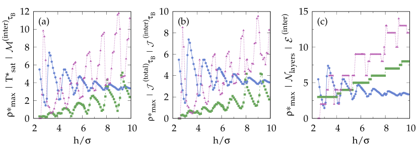
Figure 8: (Color online). The maximum value of density peaks $\rho_{\rm max}^{*}$ [solid squares in (a), (b) and (c)], the scaled saturation time $T_{\rm sat}^{*}\times 10^{-3}$ [open circles in (a)], the scaled maximum value of the interlayer fluxes, ${\cal M}^{(\rm inter)}\tau_{B}\times 8\cdot 10^{2}$ [gray triangles in (a)], the scaled total interlayer flux ${\cal J}^{(\rm inter)}\tau_{B}\times 80$ [gray triangles in (b)], the scaled total flux ${\cal J}^{(\rm total)}\tau_{B}\times 0.025$ [open circles in (b)], the number of extrema of interlayer fluxes ${\cal E}^{(\rm inter)}$ [gray triangles in (c)], and the total number of layers ${\cal N}_{\rm layers}$ [open circles in (c)] as a function of the cell dimension $h/\sigma$ corresponding to the dynamic evolution from a constant density initial profile with $\eta_{0}=0.6$.

Now we describe in detail the correlations between the different quantities (defined in Sec. II.2) that characterize the dynamics as the cell dimension $h/\sigma$ is varied. In Fig. 8(a) we show the maximum of the equilibrium density profile at the cell, $\rho_{\rm max}$, the saturation time $T_{\rm sat}$, and the maximum value of the interlayer flux ${\cal M}^{(\rm inter)}$, as a function of $h/\sigma$. The saturation times $T_{\rm sat}$ are longer for well commensurate cells containing highly localized density peaks (maxima of $\rho_{\rm max}$). By contrast, the interlayer fluxes are less important: note how the minima of ${\cal M}^{(\rm inter)}$ as a function of $h/\sigma$ are perfectly correlated with the maxima of $\rho_{\rm max}$. Therefore, (i) longer times are necessary to reach equilibrium states with highly structured density profiles, and (ii) particle localization is dominated by intralayer, as opposed to interlayer, fluxes.

This scenario is clear from Fig. 8(b), where we can see that the maxima of the total interlayer flux ${\cal J}^{(\rm inter)}$ correspond to poorly commensurate cells; equilibrium profiles with smeared out peaks are obtained by strong interlayer fluxes where particles are exchanged between neighbouring layers. In contrast, well commensurate cavities reach their equilibrium states with much lower values of ${\cal J}^{(\rm inter)}$. As total fluxes ${\cal J}^{(\rm total)}$ are higher for well commensurate cavities [see panel (b)], while interlayer ones are less important, we can draw the important conclusion that intralayer fluxes are dominant during relaxation to well structured density profiles. The nonmonotonicity of interlayer fluxes are well described by their total number of extrema ${\cal E}^{(\rm inter)}$, and these is higher for well commensurate cells [see Fig. 8 (c)]. The dynamic evolution from a constant density to a K phase with highly localized density peaks is more complex: particle migration to well localized positions inside each layer with further restructuring through interlayer fluxes results in a highly nonmonotonic relaxation dynamics.

Finally it is interesting to note that rapid changes in the total number of layers ${\cal N}_{\rm layers}$ inside the cavity as $h/\sigma$ is changed take place for poorly commensurate cells with delocalized fluid-like density profiles [see Fig. 8 (c)]. We have confirmed that the rapid change in ${\cal N}_{\rm layers}$ with $h/\sigma$, although related with the commensuration first-order transitions of a confined K phase inside a cavity with hard boundaries miguel3 , does not imply a phase transition. When hard walls are substituted by soft walls these transitions are suppressed.

III.2 Dynamic evolution from a C density profile

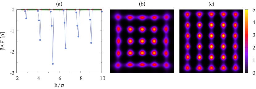
Figure 9: (Color online). Free-energy differences [(a)] between asymmetric [(c)] and symmetric [(b)] finally converged density profiles. The latter are those corresponding to $h/\sigma=6.6$ resulting from the DDF evolution of confined PHS with initial density profiles corresponding to constant (b) and to bulk equilibrium C (c) density profiles, both having a mean packing fraction $\eta_{0}=0.57$.

In this section we report on the differences between final states when the initial conditions are changed. For a cell with size $h/\sigma=6.6$, we choose initial profiles corresponding to uniform density, Fig. 9 (b), and bulk equilibrium C phase, Fig. 9 (c). In the first case, panel (b), the final state is identical as before –a symmetric K phase with layers formed by the same number of particles along $x$ and $y$ directions. In the second, an asymmetric density profile is obtained, as shown in panel (c). Note that the number of particles in layers along the $y$ axis is one more than that along the $x$-axis. These asymmetric density profiles are always obtained when $h$ is very well commensurate with the lattice parameter, $a_{\rm C}$, of the C phase at bulk, i.e. when $h/a_{\rm C}\simeq k\in\mathbb{N}$. At this packing fraction the C phase is stable at bulk. If the cell size is such that an integer number of layers can be accommodated, then the total free energy will be lower than that of the symmetric density profile, panel (b). However the main effect of the external potential, as pointed out before, consists of the localization of particles at the nodes of a regular lattice (of rectangular symmetry for asymmetric density profiles). Therefore, starting from a C density profile the system evolves by keeping the same number of C layers along the $x$ direction (and consequently by fixing the lattice parameter along this direction to be $a_{\rm C}$), with a further localization of particles by diffusion along $y$ (parallel to the C layers) to their final positions. These positions are such that the lattice parameter is close to $a_{\rm K}$ (that of the metastable K phase at bulk) along the $y$ axis.

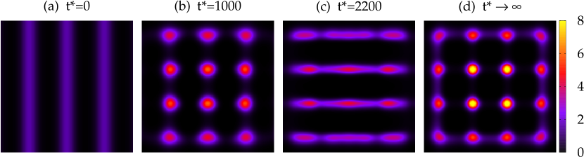
Figure 10: (Color online). Density profiles corresponding to the dynamical evolution from a C initial profile at $t^{*}=0$ (a), $t^{*}=1000$ (b), $t^{*}=2200$ (c) and $t^{*}\to\infty$ (d) inside a cavity of $h/\sigma=4.3$.

Asymmetric density profiles, such as that in panel (c), are obtained only for special cells that commensurate with $a_{\rm C}$. However, when this occurs, their free energies are lower than that corresponding to the (metastable) K-symmetric profile [panel (b)]. This is shown in panel (a), where the free-energy difference $\beta\Delta{\cal F}[\rho]\equiv\beta\left({\cal F}\left[\rho^{(\rm asym)}\right]-{\cal F}\left[\rho^{(\rm sym)}\right]\right)$ is plotted as a function of $h/\sigma$. The blue circles, corresponding to nonzero values, pertain to asymmetric density profiles, while the green triangles correspond to converged K-symmetric density profiles. Red squares indicate values of cavity size $h/\sigma$ for which a long-time dynamical evolution occurs; they are values with similar commensuration of $h/a_{\rm C}$ and $h/a_{\rm K}$, so that the system, depending on the initial conditions, could be arrested for a long time in metastable states. To illustrate this behaviour, Fig. 10 shows density profiles at four different times. Panel (a), the initial condition, consists of a C density profile with three layers inside a cavity of $h/\sigma=4.3$. Fig. 11(a) shows the interlayer fluxes for the same system. As we can see from Fig. 10(b), the system initially evolves by localizing four different K peaks along each of the C layers, changing the density profile to an asymmetric K phase and selecting the distance between peaks along the $y$ direction to optimise the commensuration with $a_{\rm K}$. This evolution occurs up to $t^{*}\sim 1000$ [see Fig. 11 (a)]. However the free energy of this asymmetric metastable state is slightly above that corresponding to the $4\times 4$ symmetric K phase, and the system continues its evolution by further delocalizing the K peaks along $x$, creating four C layers parallel to this direction [see Fig. 10 (c)]. This process lasts up to $t^{*}\sim 2000$ [see Fig. 11 (a)] from which takes place the last dynamical path: the localization of four K peaks within each C layer to end in a $4\times 4$ symmetric K profile [see Fig. 10 (d)]. Thus, we can conclude that, for some special values of $h/\sigma$, the system can dynamically be trapped in metastable states ($3\times 4$ K profile for $h/\sigma=4.3$) during a long period of time ($\sim 1000\tau_{B}$). For larger cavity sizes this effect is more dramatic, as can be seen in Fig. 11(b), where we show the interlayer fluxes corresponding to the dynamical evolution from a C phase with 7 layers up to the final equilibrium $8\times 8$ K profile inside a cavity of $h/\sigma=9.1$. We can see that the system is arrested into a $7\times 8$ K profile during $\sim 30000\tau_{B}$ after which the density profile is symmetrized through its columnarization along $x$ with a further localization of 8 K peaks along the columns to end in the symmetric $8\times 8$ density profile.

Figure 11: Interlayer fluxes corresponding to a dynamical evolution from C density profiles inside cavities of $h/\sigma=4.3$ (a) and 9.1 (b).

III.3 Dynamic evolution from a K density profile

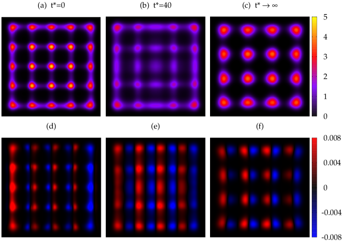
Figure 12: (Color online). The initial (a), intermediate (b) and finally converged (c) density profiles both with $\eta_{0}=0.6$. The initial density profile was conveniently scaled to fit it inside the cavity of $h/\sigma=5.1$. The fluxes $J_{x}({\bf r})$ are also plotted for times close to the initial (d), intermediate (e) and final (f) states. In (e) and (f) fluxes have been multiplied by factors of 3 and 40, respectively.

In preceding sections we described the dynamic evolution of confined PHS from F-like or C-like nonequilibrium initial conditions to their final states consisting of symmetric or asymmetric K-like density profiles. Now we proceed to describe the dynamics that follows our system departing from a non-equilibrium confined K-like symmetric density profile compressed enough that its total number of layers is one more than that corresponding to the equilibrium situation. The initial density profile was taken from the already converged density profile corresponding to a wider cell and conveniently scaled along to $x$ and $y$ directions to fit it to the boundaries of the new cell. Also it is multiplied by a constant factor to fix to 0.6 the mean packing fraction over the cell. In Fig. 12 we present the results corresponding to the cell of dimensions $h/\sigma=5.1$ and taking an initial density profile corresponding to the equilibrium one of a cavity with $h/\sigma=5.8$ properly scaled. The panels (a), (b) and (c) correspond to the initial ($t^{*}=0$), intermediate ($t^{*}=40$), and finally converged ($t^{*}\to\infty$) density profiles, while in (d), (e) and (f) panels we present the $x$-component of the local flux, $J_{x}({\bm{r}},t)$, for the same times.

We have found the following evolution from a three-layer density profile: (i) The density profile in the central square chains is delocalized over space, creating a smeared-out density profile along these directions, (ii) the rest of the peaks, even those corresponding to the most external (in contact with the soft wall), also delocalize along $x$ and $y$ directions and they move to the center of the cell creating an effective flux and (iii) the density profile is then restructured from the fluid-like density profile to the final one with only two, instead of three, layers and without any peak at the centre of the cell. This scenario is confirmed by the evolution of the fluxes: note in (e) how the highest values of the fluxes are located in the neighborhood of the central chains. As we have already discussed above the identification of a peak as a particle could be misleading. The density profiles shown in (a) and (c) have a total amount of 25 and 16 peaks. However the mean packing fraction is the same ($\eta_{0}=0.6$) for both. This difference can be explained due to a higher fraction of vacancies in the $4\times 4$ density profile. Note that if we approximately parameterize it as

$$\rho({\bm{r}})\simeq(1-\nu)\left(\frac{\alpha}{\pi}\right)^{3/2}\sum_{{\bm{R}}_{\bm{k}}\in{\cal L}}e^{-\alpha\left({\bm{r}}-{\bm{R}}_{\bm{k}}\right)^{2}},$$ (30)

where $\nu$ is the fraction of vacancies, $\alpha$ is the Gaussian parameter which takes into account the extent of particle fluctuations around the positions ${\bm{R}}_{\bm{k}}$ of the square lattice ${\cal L}$, then the mean packing fraction can be approximately calculated as

$$\eta_{0}\simeq\frac{N_{\rm peaks}}{A_{\rm cell}}\int_{a_{0}}d{\bm{r}}\rho({\bm{r}})\sigma^{2}\simeq\frac{N_{\rm peaks}(1-\nu)\sigma^{2}}{A_{\rm cell}}.$$ (31)

with $a_{0}$ the unit cell containing at most one particle. $\eta_{0}$ being the same for both density profiles with different number of peaks, $N_{\rm peaks}^{(1)}=25$ and $N_{\rm peaks}^{(2)}=16$, allow us to obtain the relation $\nu^{(1)}=\left(9+16\nu^{(2)}\right)/25$ between the fraction of vacancies. If we suppose that the density profile with 16 peaks has zero vacancies ($\nu^{(2)}=0$) we obtain a $36\%$ ($\nu^{(1)}=9/25$) of vacancies for the 25-peaks density profile.

The behavior of particle fluxes during the dynamics from 25 to 16 peaks can be seen in Fig. 12. Panel (d) shows the $x$-component of the flux, $J_{x}({\bm{r}},t)$, at the instant $t\approx 0$. The other $y$-component has, by symmetry, exactly the same behavior and can be obtained from the $x$-component by a $90^{\circ}$ rotation. We can see how the layers close to the soft-walls move to the center of the cell (the direction of fluxes of left and right extremal layers point to the right and to the left respectively). Moreover the peaks belonging to the intermediate chain is asymmetrically decomposed by diffusion to left and right creating and effective flux to the centre of the cell. The same occurs with the central peak which is symmetrically smeared out by diffusion. At further times the density profile becomes fluid-like over the whole cell (except for the external layer which keeps certain structure) and then it is reconstructed to get a total amount of 16 peaks. In panel (f) we show the spatial inhomogeneities of $J_{x}({\bm{r}},t_{2})$ (for $t_{2}\approx T_{\rm sat}$) close to the equilibrium: During the last steps of peaks formation a set of pairs of fluxes of much less magnitude coming from both, left and right, directions converge to the 16 particle positions.

IV C/K nucleation induced by the presence of obstacles

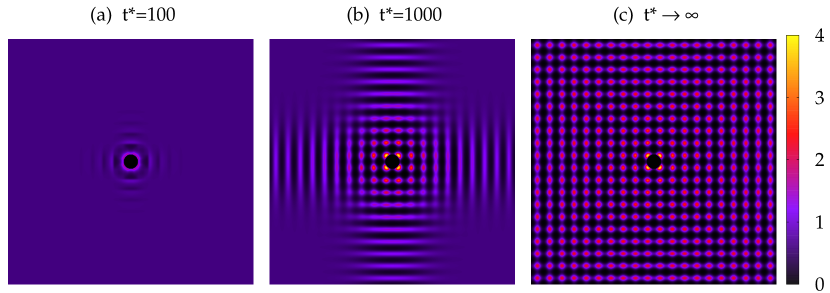
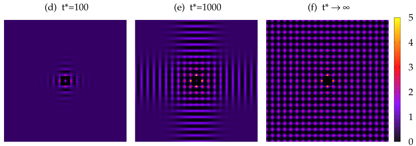
Figure 13: (Color online). A sequence of three density profiles $\rho^{*}({\bm{r}},t)$ following the dynamics from the DDFT. The profiles correspond to three different times (as labeled) during the crystallization of PHS around a circular obstacle of diameter $D=\sigma$ (a)-(c) and a square obstacle of side length and $D=1.5\sigma$ (d)-(f). The initial density profile was taken constant with packing fraction $\eta_{0}=0.6$ while periodic boundary conditions were used.

This section is different from the previous ones in one important aspect: the kind of external potential used to promote the heterogeneous nucleation of K or C phases. We have introduced a strong repulsive potential inside a spatial region of circular, square, rectangular or triangular symmetries, with the aim of mimicking a hard obstacle at the centre of the box. The obstacle size was chosen to have a few lattice parameters, $q\sigma$ ($q\in\mathbb{Q},\ 1\leq q\leq 12$), and periodic boundary conditions were used. The size of the square box, $h$, inside which the DDFT equation is numerically solved was selected large enough to guarantee the correct relaxation of the density profiles at long distances from the obstacle. Also, the specific value of $h$ was selected at a local minimum of the oscillatory free-energy profile as a function of $h$. The main purpose here is to study the dynamics of the heterogeneous nucleation promoted by the presence of obstacles with different symmetries.

First, we use obstacles with different geometries but with the property that they have at least fourfold rotational symmetry (i.e. they are invariant under rotations of $90^{\circ}$). These are the circular and the square obstacles. In Fig. 13 we present a sequence of three density profiles, $\rho({\bf r},t_{i})$ ($t_{1}<t_{2}<t_{3}=T_{\rm sat}$), following the dynamic evolution to equilibrium from a constant-density initial condition (with $\eta_{0}=0.6$) and for external potentials of circular (a)-(c) and square symmetries (d)-(f); these potentials mimic strong repulsive objects of sizes $D=\sigma$ and $1.5\sigma$ (corresponding to the values of diameter and side-length, respectively).

The first stages in the dynamics consist of the propagation of four symmetric fronts of C ordering along the two perpendicular ($x$ and $y$) directions. These fronts propagate with finite velocity from the obstacle to the box boundaries (see Fig. 13). Obviously the four fronts form an square wave and local maxima of the density profile are located, by interference effects, at the corners of the square front. The heterogeneity of the density profile along the front induces a secondary mechanism which takes place at longer times: the localization of particles by migration along the perimeter of the square front to their final equilibrium locations at the nodes of a simple square lattice of lattice parameter $a_{\rm K}$ (corresponding to a metastable K phase at bulk). Note that, for this density $\eta_{0}$, the stable phase is C, but the obstacle stabilizes the K phase. The dynamics of PHS around an obstacle with circular or square symmetries are similar, as can be seen from the figure. The relevant variable that determines the final structure of the K phase is the diameter of the obstacle; for a circle with $D=\sigma$, panels (a)-(c), values of density peaks in contact with the obstacle are higher than the rest. Also, a line joining these peaks outlines the unit cell of the simple square lattice of the metastable K phase. For a square obstacle of similar size the structure (not shown) is identical: the highest density peaks are located at the corners of the square obstacle. By increasing the size of the obstacle up to $D=1.5\sigma$ one obtains the final structure shown in panel (f). Now the square outlined by the density peaks in contact with the obstacle is larger than the unit cell and rotated $45^{\circ}$ with respect to the $x$ axis. The presence of the obstacle generates a vacancy of just one particle at its centre while for $D=\sigma$ the structure is defect-free. Again the same density profile is generated for a circular obstacle of diameter $D=1.5\sigma$.

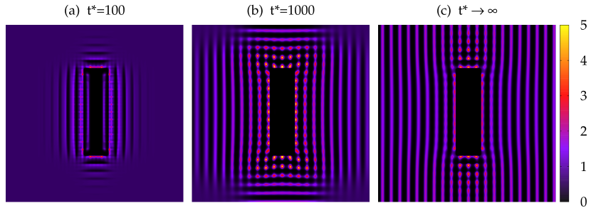
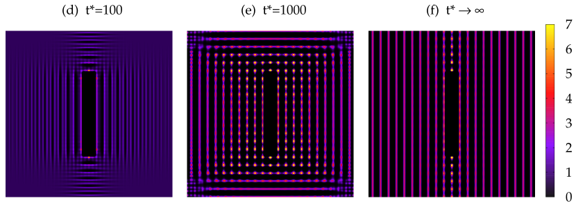
Figure 14: (Color online). A sequence of density profiles $\rho^{*}({\bm{r}},t)$ corresponding to three different times (as labeled) during the columnarization of PHS around a rectangular obstacle of width ($D$) and length ($L$) equal to $(D,L)=(3.15,12)\sigma$ (a)–(c) and $(D,L)=(1.65,12)\sigma$ (d)–(f). The initial density profiles were taken constant with $\eta_{0}=0.6$ (a)–(c) and $\eta_{0}=0.75$ (d)–(f).

The second study concerns the dynamics of heterogeneous formation of C/K phases around an obstacle without the fourfold symmetry. We analyse two obstacles. The first is a rectangle with a long side-length of $L=12\sigma$, and short side-lengths of $D=3.15\sigma$ and $D=1.65\sigma$. The other is an equilateral triangle of side-length $D=3\sigma$. A sequence of density profiles obtained during the dynamic evolution, taken at three different times, are shown in Figs. 14(a)–(c) and (d)–(f) for rectangular obstacles with $D=3.15\sigma$ and $D=1.65\sigma$, respectively, and in Fig. 16 (a)–(c) for the triangular obstacle. As can be seen, the rectangle stabilizes a C phase, with columns parallel to the longest side of the rectangle. Interestingly, after a time where a rectangular front of C symmetry is propagated from the obstacle, a further localization of particles takes place. This localization proceeds by particle migration along the perimeter of the front, similar to the cases with obstacles of circular and square geometries, and extends up to three layers from the obstacle for $D=3.15\sigma$ and to the whole area for $D=1.65\sigma$. There is however an important difference in this case: after the second stage, particles again delocalize, restoring the C layers parallel to the long side-length. Therefore equilibrium profiles correspond to a defected C phase with disrupted columns (three or one layer for $D=3.15\sigma$ and $D=1.65\sigma$, respectively, as shown in Fig. 14) formed by particles with some degree of localization. No perfect commensuration between the difference $h-D$ (with $h$ the width of the box) and the lattice parameter $a_{\rm C}$ corresponding to the stable C phase at bulk, as it occurs for $D=3.15\sigma$, generates a deformation of columns around the obstacle [see panel (c)].

The symmetry of the final equilibrium density profile that growths from a rectangular obstacle, considering a constant initial density profile with $\eta_{0}$ slightly above its bulk C-K value, strongly depends on $D$. Selecting $D$ well or not well commensurated with $a_{\rm C}$ we obtain as $t\to\infty$ density profiles with C or K symmetries respectively as they are shown in Fig. 15.

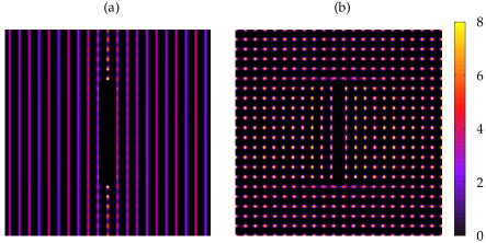
Figure 15: (Color online). Equilibrium density profiles as obtained from the final converged states of the dynamic evolution following the DDFT and considering a constant density initial profile with $\eta_{0}=0.75$. The presence of a rectangular obstacle of length $L=12\sigma$ and width $D=1.65\sigma$ (a) and $1.14\sigma$ (b) are imposed for $t\geq 0$ through a corresponding external potential.

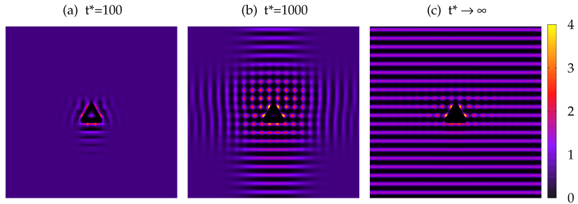
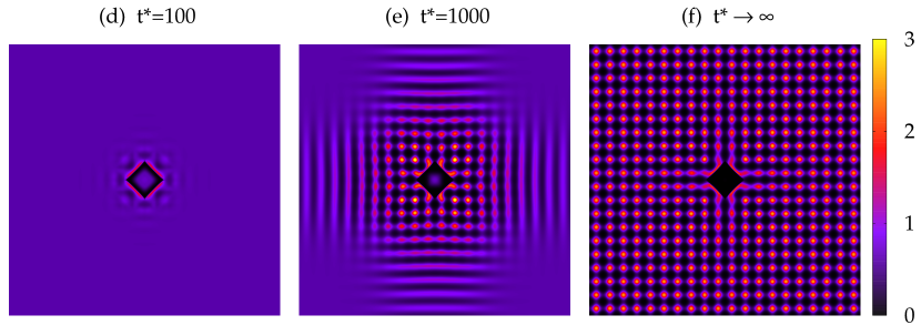
Figure 16: (Color online). A sequence of density profiles $\rho^{*}({\bm{r}},t)$ corresponding to three different times (as labeled) during the crystallization of PHS around: (a)-(c) an equilateral triangle of side-length $D=3\sigma$ with one of its sides parallel to the $x$-axis, and (d)-(f) a square rotated by 45^∘ and with side length $D=2.6\sigma$. The initial density profile was constant, with $\eta_{0}=0.6$.

Another example of an obstacle without the fourfold symmetry is an equilateral triangular obstacle which obviously has a $60^{\circ}$ rotational symmetry. We have found that a stable C phase is induced at $\eta_{0}=0.6$ when one of the triangle sides is parallel to $x$ or $y$-Cartesian axes (the same directions of the lattice vectors). The set of three density profiles during the evolution dynamic is shown in Fig. 16 (a)-(c). We again see: (i) a first propagation of three triangular C fronts with their further reorientation to form four fronts in the two mutual perpendicular directions at larger distances, (ii) a further localization of particles around the nodes of a square lattice which extend to few layers from the obstacle, and (iii) the final delocalization of particles along the C layers, except for some particles in the neighborhood of the contact between the columns and the obstacle.

To end this section we show the results of the dynamics of heterogeneous crystallization induced by the presence of a $45^{\circ}$ rotated square obstacle with respect to the lattice vectors of the K phase. The results are shown in Fig. 16 (d)-(f). Again this is an example of an obstacle with fourfold symmetry and again we obtain a dynamic behavior similar to that corresponding to the non-rotated square. The only differences consist on the very initial steps of the dynamics evolution when four rhombus-like fronts depart from the obstacle while the other difference is related to the particle distribution close to the obstacle at equilibrium. See in panel (f) for $t\to\infty$ the presence of four fluid-like layers close to the square sides which are deformed to connect the $x$ and $y$ lattice directions.

V Conclusions

We have used the DDF formalism, based on the FMT for a fluid of PHS, to study the dynamics of heterogeneous nucleation of the K phase when the fluid is confined by soft-repulsive walls. The walls define a lattice of periodically spaced square cells that confine the fluid. The study is divided into three parts, each corresponding to a specific initial condition: (i) constant density profile, (ii) density profile with C symmetry and (iii) density profile with K symmetry. We have characterized the dynamics using different quantities, such as saturation time, interlayer fluxes and their maximum value and total number of extrema, and total (interlayer plus intralayer) fluxes. These quantities are analysed as a function of cell size and correlated with some features of the equilibrium density profile, such as absolute maximum over the cell and total number of layers.

We found that, for poorly commensurate cells (i.e. with a lattice parameter incommensurate with that of a metastable K phase at bulk), the structure of the density profile consists of smeared-out peaks with values lower that those for well-commensurate cavities. In addition, the dynamics is dominated by strong interlayer fluxes which expel particles from the walls to the interior of the cavity. The equilibrium configuration is reached by further interchange of particles between neighbouring layers, resulting in moderately localized peaks. By contrast, in the case of well-commensurate cells, intralayer fluxes are dominant, with particles localising at the nodes of the simple square lattice. Although interlayer fluxes are lower for well-commensurate cavities, they exhibit a more complex behaviour: strong non-monotonicity with presence of a high number of extrema, and damping oscillations which increase the saturation time before equilibrium is reached. This highly non-linear behaviour strongly correlates with longer saturation times, which dramatically increase with number of layers. As a function of cell size, this number exhibits a rapid increase for the most noncommensurate cavities (those containing a fluid-like density profile). However we have checked that this abrupt increase does not imply a phase transition, which is discarded due to the soft character of the external potential.

When the dynamics departs from a C density profile, in most cases the final state is the usual symmetric K phase. However, for some special cells, in particular those which commensurate with the C period at bulk, the equilibrium state is an asymmetric K phase in which layers have a different number of peaks along the $x$ and $y$ directions. When this occurs, the free energy of the asymmetric profile is lower. Finally, we also used previously converged symmetric K-phase density profiles scaled to the new cell as initial condition. We observed the delocalization of density peaks and the presence of asymmetric fluxes of particles from the walls to the center, with inner layers being the first to melt. Further reconstruction of density peaks from a fluid-like profile gives rise to a lower number of layers, but these are well commensurate with cell size.

A final study concerns the dynamics of heterogeneous growth of C or K phases from a obstacle with circular, square, triangular or rectangular symmetry. The K phase grows from obstacles with circular or square symmetries, since they have the same fourfold symmetry. By contrast, when obstacles do not have fourfold symmetry and they reasonably commensurate with the C-phase lattice parameter, the final equilibrium state is generally a C phase, with layers parallel to the long side length of the rectangle or to one of the triangular sides. However, the dynamics in this case is far from simple. Density waves of C symmetry propagate from the obstacle with further localization of particles along these fronts; these waves extend to a few layers or even to the whole area. Finally, particles localize more strongly, until a regular K square lattice is created (for circular and square objects), or they delocalize again to recover the C phase, which is the final equilibrium state (for rectangular and triangular objects).

- (1) Dynamic density functional theory of fluids, U. M. B. Marconi and P. Tarazona, J. Chem. Phys. 110, 8032 (1999).
- (2) A dynamic density functional theory for particles in a flowing solvent, M. Rauscher, A. Dominguez, M. Kruger, and F. Penna, J. Chem. Phys. 127, 244906 (2007).
- (3) Dynamic density functional theory for steady currents: Application to colloidal particles in narrow channels, F. Penna and P. Tarazona, J. Chem. Phys. 119, 1766 (2003).
- (4) Ultrasoft colloids in cavities of oscillating size or sharpness, M. Rex, C. N. Likos, H. Löwen, and J. Dzubiella, Mol. Phys. 104, (2006).
- (5) Soft colloids driven and sheared by traveling wave fields, M. Rex, H. Löwen, and C. N. Likos, Phys. Rev. E 72, 021404 (2005).
- (6) Vacancy diffusion in colloidal crystals as determined by dynamical density-functional theory and the phase-field-crystal model, S. van Teeffelen, C. V. Achim, and H. Löwen, Phys. Rev. E 87, 022306 (2013).
- (7) Classical density functional theory: an ideal tool to study heterogeneous crystal nucleation, G. Kahl and H. Löwen, J. Phys.: Condens. Matter 21, 464101 (2009).
- (8) Colloidal crystal growth at externally imposed nucleation clusters, S. van Teeffelen, C. N. Likos, and H. Löwen, Phys. Rev. Lett. 100, 108302 (2008).
- (9) Nonequilibrium sedimentation of colloids on the particle scale, C. P. Royall, J. Dzubiella, M. Schmidt, and A. van Blaaderen, Phys. Rev. Lett. 98, 188304 (2007).
- (10) Dynamics of fluid mixtures in nanospaces, U. M. B. Marconi, and S. Melchionna, J. Chem. Phys. 134, 064118 (2011).
- (11) Modeling diffusion in colloidal suspensions by dynamical density functional theory using fundamental measure theory of hard spheres, D. Stopper, K. Marolt, R. Roth, and H. Hansen-Goos, Phys. Rev. E 92, 022151 (2015).
- (12) Dynamical and structural insights into the smectic phase of rod-like particles, E. Grelet, M. P. Lettinga, M. Bier, R. van Roij, and P. van der Schoot, J. Phys. Condens. Matter 20, 494213 (2008).
- (13) Dynamical and structural insights into the smectic phase of rod-like particles, E. Grelet, M. P. Lettinga, M. Bier, R. van Roij, and P. van der Schoot, J. Phys. Condens. Matter 20, 494213 (2008).
- (14) Aggregation of self-propelled colloidal rods near confining walls, H. H. Wensink and H. Löwen, Phys. Rev. E 78, (2008).
- (15) Monolayers of hard rods on planar substrates. II. Growth, M. Klopotek, H. Hansen-Goos, M. Dixit, T. Schilling, F. Schreiber, and M. Oettel, J. Chem. Phys. 146, 084903 (2017).
- (16) Particle conservation in dynamical density functional theory, D. de las Heras, J. M. Brader, A. Fortini, and M. Schmidt, J. Phys.: Condens. Matter 28, 244024 (2016).
- (17) Free energy models for nonuniform classical fluids, J. K. Percus, J. Stat. Phys. 52, 1157 (1988).
- (18) Dimensional Crossover of the Fundamental-Measure Functional for Parallel Hard Cubes, J. A. Cuesta and Y. Martínez-Ratón, Phys. Rev. Lett. 78, 3681 (1997).
- (19) Fundamental measure theory for mixtures of parallel hard cubes. I. General formalism, J. A. Cuesta and Y. Martínez-Ratón, J. Chem. Phys. 107, 6379 (1997).
- (20) Fundamental measure theory for hard disks: Fluid and solid, R. Roth, K. Mecke, and M. Oettel, J. Chem. Phys. 136, 081101 (2012).
- (21) Density functional theory for hard-sphere mixtures: the White Bear version mark II, H. Hansen-Goos and R. Roth, J. Phys.: Condens. Matter 18, 8413 (2006).
- (22) Free-energy model for the inhomogeneous hard-sphere fluid mixture and density-functional theory of freezing, Y. Rosenfeld, Phys. Rev. Lett. 63, 980 (1989).
- (23) Phase-field-crystal models for condensed matter dynamics on atomic length and diffusive time scales: an overview, H. Emmerich, H. Löwen, et. al., Adv. Phys. 61, 665 (2012).
- (24) Dynamical density functional theory with hydrodynamic interactions in confined geometries, B. D. Goddard, A. Nold, and S. Kalliadasis, J. Chem. Phys. 145, 214106 (2016).
- (25) Phase behaviour and correlations of parallel hard squares: From highly confined to bulk systems, M. González-Pinto, Y. Martínez-Ratón, S. Varga, P. Gurin, and E. Velasco, J. Phys.: Condens. Matter 28, 244002 (2016).
- (26) Free minimization of the fundamental measure theory functional: Freezing of parallel hard squares and cubes, S. Belli, M. Dijkstra, and R. van Roij, J. Chem. Phys. 137, 124506 (2012).
- (27) Liquid-crystal patterns of rectangular particles in a square nanocavity, M. González-Pinto, Y. Martínez-Ratón, and E. Velasco, Phys. Rev. E 88, 032506 (2013).