Rayleigh-Bénard convection in a creeping solid with melting and freezing at either or both its horizontal boundaries

Abstract

Solid state convection can take place in the rocky or icy mantles of planetary objects and these mantles can be surrounded above or below or both by molten layers of similar composition. A flow toward the interface can proceed through it by changing phase. This behaviour is modeled by a boundary condition taking into account the competition between viscous stress in the solid, that builds topography of the interface with a timescale $\tau_{\eta}$, and convective transfer of the latent heat in the liquid from places of the boundary where freezing occurs to places of melting, which acts to erase topography, with a timescale $\tau_{\phi}$. The ratio $\Phi=\tau_{\phi}/\tau_{\eta}$ controls whether the boundary condition is the classical non-penetrative one ($\Phi\rightarrow\infty$) or allows for a finite flow through the boundary (small $\Phi$). We study Rayleigh-Bénard convection in a plane layer subject to this boundary condition at either or both its boundaries using linear and weakly non-linear analyses. When both boundaries are phase change interfaces with equal values of $\Phi$, a non-deforming translation mode is possible with a critical Rayleigh number equal to $24\Phi$. At small values of $\Phi$, this mode competes with a weakly deforming mode having a slightly lower critical Rayleigh number and a very long wavelength, $\lambda_{c}\sim 8\sqrt{2}\pi/3\sqrt{\Phi}$. Both modes lead to very efficient heat transfer, as expressed by the relationship between the Nusselt and Rayleigh numbers. When only one boundary is subject to a phase change condition, the critical Rayleigh number is $\mbox{{Ra}}_{c}=153$ and the critical wavelength is $\lambda_{c}=5$. The Nusselt number increases about twice faster with Rayleigh number than in the classical case with non-penetrative conditions and the average temperature diverges from $1/2$ when the Rayleigh number is increased, toward larger values when the bottom boundary is a phase change interface.

1 Introduction

Rayleigh-Bénard convection is one of the main heat transfer mechanisms in natural sciences, responsible for most of the dynamics of the atmosphere and oceans (Pedlosky, 1987), plate tectonics (Schubert et al., 2001), dynamo action in planetary cores (Roberts & King, 2013). It is also one of the most generic example of pattern formation mechanism in fluid dynamics (e.g. Cross & Hohenberg, 1993; Manneville, 2004) and has therefore attracted a lot of attention for a century since the work of Lord Rayleigh (Rayleigh, 1916). However, the mathematical and experimental studies of Rayleigh-Bénard convection have usually considered boundary conditions that are not fully relevant to the natural systems that justified them, their horizontal surfaces being generally considered as subjected to no-slip or free-slip boundary conditions. The former is valid for convection experiments in a tank and for the natural fluids bounded by much more viscous enveloppes, like the liquid cores of terrestrial planets and the bottom of the ocean. The latter is often considered as an approximation for a free-surface condition, as applies to a fluid bounded by a much less viscous one. This is in particular the case of the solid planetary mantles that, on long timescales, behave like very viscous fluids (e.g. Turcotte & Oxburgh, 1967; McKenzie et al., 1974; Jarvis & McKenzie, 1980) and are bounded below and above by liquid or gaseous layers. This approximation neglects the effect of the topography on convection and some studies have been devoted to the modeling of these effects, which can be dramatic when it is associated to, for example, intense volcanism in hot planets (Monnereau & Dubuffet, 2002; Ricard et al., 2014).

In the present paper, we consider the effects of having horizontal boundaries at which a solid-liquid phase change occurs on Rayleigh-Bénard convection in the creeping solid, that has an infinite Prandtl number (Schubert et al., 2001). For simplicity, we consider a Newtonian fluid with a uniform high viscosity, neglecting the effects of more complex rheologies (e.g. Parmentier, 1978; Christensen & Yuen, 1989; Davaille & Jaupart, 1993; Tackley, 2000; Bercovici & Ricard, 2014), that is bounded by a low viscosity liquid of the same composition as the convecting solid. The boundary between the liquid and the solid consists of a phase change whose position is controlled by a Clapeyron diagram relating pressure and temperature for phase equilibrium. In the context of planetary interiors, the pressure is largely dominated by the hydrostatic contribution and the interface is on average a horizontal surface. The stress field and associated dynamic pressure due to the dynamics of the solid leads to deformation of the interface with a viscous timescale $\tau_{\eta}$. The topography creates variations of the thermal gradient on the liquid side which drives a convective heat transfer in the liquid acting to erase the topography by transporting the latent heat released by freezing in topography lows to topography highs where melting occurs. Other sources of motions in the liquid can also contribute to this lateral heat transfer which happens on a timescale $\tau_{\phi}$, the expression of which being derived in section 2. The ratio of the two timescales, $\Phi=\tau_{\phi}/\tau_{\eta}$, controls the behaviour of the boundary. For a large value of $\Phi$, the topography is set by the balance between the viscous stress in the solid and the buoyancy of the topography, the phase change acting on a too long timescale to affect the classical behaviour of the free surface. The buoyancy of the topography is responsible for making the vertical velocity drop to zero at the interface, which leads to an effectively non-penetrating boundary condition. On the other hand, for low values of $\Phi$, the topography is erased by freezing and melting at a rate greater than the one at which it is generated. The removal of the associated buoyancy leads to a non-null velocity across the interface.

This situation has already been considered in the case of the dynamics of the Earth inner core (Alboussière et al., 2010; Monnereau et al., 2010; Deguen et al., 2013; Mizzon & Monnereau, 2013), which is the solid iron sphere at the center of the liquid iron core of the Earth. Deguen et al. (2013) have derived a general formulation of the boundary condition for arbitrary values of $\Phi$ and shown that the application of this boundary condition to a sphere considerably changes the dynamics by decreasing the critical Rayleigh number for the onset of thermal convection and allowing a new mode of convection, the translation mode, where no deformation occurs in the sphere, melting happens at the boundary of the advancing hemisphere and freezing occurs at the trailing boundary.

A similar situation arises for the ice shell of some satellites of giant planets in the solar system which are believed to host a liquid ocean below their ice layer (Pappalardo et al., 1998; Khurana et al., 1998; Gaidos & Nimmo, 2000; Tobie et al., 2003; Soderlund et al., 2014; Čadek et al., 2016). Some of the largest of such satellites can also have a layer of high pressure ices below their ocean (Grasset et al., 2000; Sohl et al., 2003; Baland et al., 2014). Another situation that implies such a melt-solid interface arises on all terrestrial planets in their early stage when their silicate layer is completely or largely molten owing to the high energy of their accretion (Solomatov, 2007; Elkins-Tanton, 2012). Convection can start in the solid mantle during its crystallisation from the magma ocean, while a liquid layer persists above and/or below (Labrosse et al., 2007). It is therefore interesting to consider convection in a layer, not a full sphere, when a phase change boundary condition applies at either or both its horizontal boundaries.

Deguen (2013) performed such a study in the case of a spherical shell with a central gravity linearly varying with radial position and showed that, again, a translation mode is possible and favoured in the linear stability analysis if both the upper and lower boundaries allow an easy phase change, that is if each has a low value of the $\Phi$ parameter. The purpose of the present paper is to extend the analysis to the plane layer situation and perform the linear stability and weakly non-linear analysis as a function of the phase change parameters of both horizontal boundaries.

The boundary conditions are presented in section 2, section 3 presents the translation mode of convection, section 4 presents the linear and weakly non-linear analysis in the case when both horizontal boundaries have the same value of the phase change parameter and section 5 shows the case when phase change is only allowed on one boundary.

2 Conservation equations and boundary conditions

Figure 1: Definition of the topography (exaggerated here for clarity) and the temperature for the boundary conditions. The dash-dotted lines are the reference positions for the conductive motionless solutions of the top and bottom boundaries. The right panel shows the reference temperature profile (thick solid line) intersecting the melting temperature at the top and bottom (thin solid lines) at temperatures $T^{+}$ and $T^{-}$, respectively. Lateral variations of the topography make the intersection deviate laterally in temperature. Representative temperature profiles in the liquid sides are shown as dashed lines. In the context of planetary applications, the temperature profiles should be interpreted as deviations from the isentropic reference.

We consider a layer of creeping solid that behaves like a Newtonian fluid on long timescales and that is bounded above or below or both by a liquid related to the solid by a phase change (fig. 1). The temperature field at rest is solution of the thermal conduction problem with temperatures at the boundaries, $T^{+}$ at the top and $T^{-}$ at the bottom, that each equals the melting temperature $T_{m}$ at the relevant pressure. Pressure, in the context of planetary interiors, is largely dominated by the hydrostatic part. The melting temperature therefore mainly depends on the vertical coordinate. The possibility of crossing the melting temperature at both the top and bottom of our computational domain requires either a non-linear dependence of $T_{m}$ on pressure or, more easily, a compositional difference between the solid and both upper and lower liquid layers (Labrosse et al., 2007). For simplicity here, we do not consider the dynamical effects of compositional variations. The vertical dependence of the melting temperature is linearised around the reference positions of the boundaries, owing to the smallness of their topographies compared to the total thickness of the layer, $d$.

The conduction temperature profile that is used as reference writes

$$T_{0}=\frac{T^{+}+T^{-}}{2}+\frac{z}{d}\left(T^{+}-T^{-}\right),$$ (1)

the reference for the vertical position $z$ being at the center of the domain. Deviations from the conduction temperature profiles are made dimensionless using $\Delta T=T^{-}-T^{+}$ as reference and denoted by $\theta$. In the following, superscripts ⁺ and ^- are used for quantities pertaining to the top and bottom boundaries, respectively, and omitted in equations that apply to both boundaries.

The crossing positions of the conduction solution with the melting temperature at the top and bottom are used as reference around which a topography height, $h^{+}$ and $h^{-}$, is defined for each boundary, respectively (fig. 1). These topographies can have either sign, positive upward, and need not average to 0, as will be shown below. At each phase change interface, two thermal boundary conditions are necessary to account for the moving boundary (Crank, 1984). The temperature must equal the phase change temperature and the heat flux discontinuity across the interface must balance the release or consumption of latent heat, $L$ (Stefan condition). The two thermal boundary conditions write

$$T(h) =T_{m}(h),$$ (2)

$$\rho_{s}Lv_{\phi} =\llbracket q\rrbracket,$$ (3)

with $v_{\phi}$ the freezing rate, $\rho_{s}$ the density of the solid and $\llbracket q\rrbracket$ the heat flux difference between the liquid and the solid sides. These boundary conditions apply to the deformed interface and need to be projected to the reference level that is used as boundary for the computation domain. Developing equation (2) to first order in $h$ gives

$$T\left(\pm\frac{d}{2}\right)=T^{\pm}+\left(\mathinner{\dfrac{\partial{}T_{m}^{\pm}}{\partial{z}}}-\mathinner{\dfrac{\partial{}T_{0}}{\partial{z}}}\right)h^{\pm}.$$ (4)

In dimensionless form, equation (4) writes

$$\theta\left(\pm\frac{1}{2}\right)=\left(1+\frac{d}{\Delta T}\mathinner{\dfrac{\partial{}T_{m}^{\pm}}{\partial{z}}}\right)\frac{h^{\pm}}{d}.$$ (5)

In the following, we assume $h^{\pm}/d$ to be small and we apply

$$\theta=0,\qquad z=\pm\frac{1}{2}.$$ (6)

Turning to the second thermal boundary condition, the discontinuity of heat flow on the right-hand-side of equation (3) is assumed to be dominated by the convective heat flow on the low viscosity liquid side, $f\sim\rho_{l}c_{pl}u_{l}\delta T_{l}$, with $\rho_{l}$ and $c_{pl}$ the density and heat capacity of the liquid, $u_{l}$ the characteristic liquid velocity and $\delta T_{l}$ the temperature difference between the boundary and the bulk of the liquid. This difference results from variations of the topography (fig. 1) and the vertical gradient of the melting temperature so that

$$f\sim-\rho_{l}c_{pl}u_{l}\left|\mathinner{\dfrac{\partial{}T_{m}}{\partial{z}}}\right|h.$$ (7)

The temperature difference $h\partial{T_{m}}/\partial{z}$ is negligible on the solid side, but crucial for the convective heat flux on the liquid side. Fig. 1 shows as dashed lines the typical local temperature profiles on the liquid side of each boundary for topography highs and lows, indicating that the implied lateral variations of heat flux density should lead to melting of regions where the solid protrudes in the liquid and freezing in depressed regions, tending toward erasion of the topography. This behaviour is ensured by the anti-correlation of $f$ and $h$ in equation (7), independently of the sign of $\dfrac{\partial{}T_{m}}{\partial{z}}$, and this applies to both top and bottom boundaries. The case of $\dfrac{\partial{}T_{m}}{\partial{z}}<0$ depicted here for the top boundary is the most usual and the opposite case depicted here for the bottom boundary is encountered for water. Note, however, that in the context of planetary applications, the temperature considered here in the liquid layers and depicted on fig. 1 is in fact the deviation from the reference isentropic temperature profile (Jeffreys, 1930; Deguen et al., 2013) and the pressure derivative of the actual melting temperature needs not be negative for having a liquid underlying the solid layer. Assuming that the convective heat flow on the liquid side dominates the right hand side of equation (3), we write

$$\rho_{s}Lv_{\phi}\sim-\rho_{l}c_{pl}u_{l}\left|\mathinner{\dfrac{\partial{}T_{m}}{\partial{z}}}\right|h.$$ (8)

The freezing rate is related to the vertical velocity $w$ across the boundary and the rate of change of the topography as

$$v_{\phi}^{\pm}=\pm\mathinner{\dfrac{\partial{}h\pm}{\partial{t}}}\mp w.$$ (9)

Combining with equation (8) gives

$$w\mp\mathinner{\dfrac{\partial{}h}{\partial{t}}}=\frac{\rho_{l}c_{pl}u_{l}}{\rho_{s}L}\left|\mathinner{\dfrac{\partial{}T_{m}}{\partial{z}}}\right|h\equiv\frac{h}{\tau_{\phi}},$$ (10)

with

$$\tau_{\phi}=\frac{\rho_{s}L}{\rho_{l}c_{pl}u_{l}\left|\dfrac{\partial{}T_{m}}{\partial{z}}\right|}$$ (11)

the characteristic phase change timescale for changing the topography by transferring latent heat from regions where it is released to places where it is consumed. $u_{l}$ depends on the dynamics of the liquid which is not solved in this paper. The uncertainty in this quantity as well as the scaling coefficients implied by the $\sim$ sign in equations (7) and (8) are all combined to make $\tau_{\phi}$ the control parameter in our study.

Across the boundaries, the total traction must be continuous. Assuming that the topography is small (i.e. the horizontal gradient of $h^{\pm}$ is small compared to 1, $|\nabla_{h}h^{\pm}|\ll 1$), this writes for the vertical component

$$-P_{s}(h^{\pm})+2\eta\mathinner{\dfrac{\partial{}w}{\partial{z}}}=-P_{l}(h^{\pm})$$ (12)

where $P$ is total pressure, $s$ and $l$ are for the solid and liquid sides, respectively, and $\eta$ is the dynamic viscosity of the solid. The total pressure on the solid and liquid sides is split into its hydrostatic part, $P(0)-\rho_{s,l}gh^{\pm}$ ($z=0$ being the reference for $h$ at each boundary) and the dynamic part $p$. On the liquid side, viscous stress and pressure fluctuations are neglected. With these assumptions, we get

$$-p+(\rho_{s}-\rho_{l}^{\pm})gh^{\pm}+2\eta\mathinner{\dfrac{\partial{}w}{\partial{z}}}=0.$$ (13)

Note that the density difference across the phase change boundary, $\Delta\rho^{\pm}=\rho_{s}-\rho_{l}^{\pm}$, takes different signs at the top and bottom since the solid must be denser than the overlying liquid but less dense that the underlying one. Therefore $\Delta\rho^{+}>0$ and $\Delta\rho^{-}<0$.

The topography at each boundary is produced as a result of total stress in the solid, with a typical timescale $\tau_{\eta}=\eta/|\Delta\rho^{\pm}|gd$ (the post-glacial rebound timescale, Turcotte & Schubert, 2001), and erased by melting and freezing, as discussed above, with a timescale $\tau_{\phi}$. Both timescales are generally much shorter than the timescale for convection in the whole domain, so that we assume that the topography adjusts instantaneously to the competition between viscous stress and phase change. Therefore, we neglect $\dfrac{\partial{}h}{\partial{t}}$ in equation (10) and combining it with equation (13) to eliminate $h^{\pm}$, we get

$$-p+\Delta\rho^{\pm}g\tau_{\phi}^{\pm}w+2\eta\mathinner{\dfrac{\partial{}w}{\partial{z}}}=0.$$ (14)

Introducing the phase change dimensionless number (Deguen et al., 2013; Deguen, 2013)

$$\Phi^{\pm}=\frac{\tau_{\phi^{\pm}}|\Delta\rho^{\pm}|gd}{\eta}$$ (15)

equation (14) takes the dimensionless form

$$\pm\Phi^{\pm}w+2\mathinner{\dfrac{\partial{}w}{\partial{z}}}-p=0,\qquad z=\pm\frac{1}{2}.$$ (16)

$\Phi^{\pm}$ is the ratio of the phase change timescale to the viscous deformation time scale. For large values of this parameter, the boundary condition (16) reduces to the usual non-penetration condition, $w=0$, while for small values it allows a non zero mass flow through the boundary. The physical interpretation is straightforward: if $\tau_{\eta}\ll\tau_{\phi^{\pm}}$, topography evolves without the possibility of the phase change to happen and is limited by its own weight that has to be supported by viscous stress in the solid. In practice, this means that the flow velocity goes to zero at the free interface and is very small at the reference boundaries $z=\pm 1/2$, which is usually modeled as a non-penetrating boundary. In the other limiting case, $\tau_{\eta}\gg\tau_{\phi^{\pm}}$, topography is removed by phase change as fast as it is created by viscous stresses and this allows a flow across the boundary.

The liquid is assumed inviscid and therefore exerts no shear stress on the convecting solid. The topography of the boundary is assumed to be small and we approximate the horizontal component of the continuity condition for traction by a free-slip boundary condition at both horizontal boundaries,

$$\mathinner{\dfrac{\partial{}u}{\partial{z}}}+\mathinner{\dfrac{\partial{}w}{\partial{x}}}=0,\qquad z=\pm\frac{1}{2}.$$ (17)

The dimensionless equations for the conservation of momentum, mass and energy are written in the classical Boussinesq approximation as

$$\frac{1}{\Pran}\left(\mathinner{\dfrac{\partial{}{\bm{v}}}{\partial{t}}}+{\bm{v}}{\bm{\cdot}}{\bm{\nabla}}{\bm{v}}\right) =-{\bm{\nabla}}p+\nabla^{2}{\bm{v}}+\mbox{{Ra}}\theta\hat{{\bm{z}}},$$ (18)

$$\bnabla\bcdot\bm{v} =0,$$ (19)

$$\mathinner{\dfrac{\partial{}\theta}{\partial{t}}}+{\bm{v}}{\bm{\cdot}}{\bm{\nabla}}\theta =w+\nabla^{2}\theta,$$ (20)

where $\Pran=\nu/\kappa$ is the Prandtl number, with $\nu$ and $\kappa$ the momentum and thermal diffusivities, ${\bm{v}}=(u,v,w)$ is the fluid velocity, $p$ is the dynamic pressure, $\mbox{{Ra}}=\alpha\Delta Tgd^{3}/\kappa\nu$ is the Rayleigh number, with $\alpha$ the thermal expansion coefficient,

and $\hat{{\bm{z}}}$ is the upward vertical unit vector. These equations have been made dimensionless using the thickness of the layer $d$ as length scale and the thermal diffusion time $d^{2}/\kappa$ as timescale.

Since we are concerned here with convection in solid, albeit creeping, layers, we will generally consider the Prandtl number to be infinite in most of the calculations below.

3 The translation mode

The boundary condition (16) discussed in the previous section permits a non-zero vertical velocity across the boundaries. If both boundaries are semi-permeable (finite values of both $\Phi^{+}$ and $\Phi^{-}$), the possibility of a uniform vertical translation arises. This situation has been explored systematically in the context of the dynamics of Earth’s inner core (Alboussière et al., 2010; Deguen et al., 2013; Mizzon & Monnereau, 2013) and in spherical shells (Deguen, 2013) but, in the case of a spherical geometry, the horizontally average vertical velocity is still null for a translation mode. Here we show that a translation mode with a uniform vertical velocity also exists in the case of a plane layer.

We search for a solution that is independent from the horizontal direction and therefore only has a vertical velocity, ${\bm{v}}=w\hat{{\bm{z}}}$. The mass conservation equation (19) implies that $w$ is independent of $z$ and we consider two situations, the linear stability problem for which $w=W\mathrm{e}^{\sigma t}$ and the steady state case for which $w$ is constant. Similarly, we can write the temperature as $\theta(z,t)=\Theta(z)\mathrm{e}^{\sigma t}$ to study the onset of convection in that mode, and $\theta$ as a function of $z$ only at steady state and similar convention for pressure as $p$ and $P$.

3.1 Linear stability analysis

The conservation equations (18)- (20) linearized around the hydrostatic state reduce to two equations

$$\frac{\sigma}{\Pran}W =-\operatorname{D\!}P+\mbox{{Ra}}\Theta,$$ (21)

$$\sigma\Theta =W+\operatorname{D\!}^{2}\Theta,$$ (22)

with $\operatorname{D\!}\equiv\dfrac{\operatorname{d\!}{}}{\operatorname{d\!}{z}}$. For neutral stability, $\sigma=0$, solving in turn equation (22) for $\Theta$ and equation (21) for $P$ subject to the boundary conditions (6) and (16) lead to

$$\left[\mbox{{Ra}}-12\left(\Phi^{+}+\Phi^{-}\right)\right]W=0.$$

A non-trivial solution for $W$ can then exist for

$$\mbox{{Ra}}=\mbox{{Ra}}_{c}=12\left(\Phi^{+}+\Phi^{-}\right),$$ (23)

which is the condition for marginal stability of the translation mode.

This system of equations can also be solved for a finite value of $\sigma$ in order to relate it to Ra. Equation (22) subject to boundary conditions $\theta(\pm 1/2)=0$ gives

$$\Theta=\frac{W}{\sigma}\left[1-2\frac{\sinh(\sigma^{1/2}/2)}{\sinh(\sigma^{1/2})}\cosh(\sigma^{1/2}z)\right]$$ (24)

Inserting this expression in Eq. (21) and solving for $P$, we obtain

$$P=cst+\left(\frac{\mbox{{Ra}}}{\sigma}-\frac{\sigma}{\Pran}\right)Wz-2\mbox{{Ra}}\,W\sigma^{-3/2}\frac{\sinh(\sigma^{1/2}/2)}{\sinh(\sigma^{1/2})}\sinh(\sigma^{1/2}z).$$ (25)

Using the boundary condition (16) at $z=1/2$ allows to determine the integration constant, which gives

$$\begin{split}P=&\Phi^{+}W+\left(\frac{\mbox{{Ra}}}{\sigma}-\frac{\sigma}{\Pran}\right)W(z-1/2)\\ &-2\mbox{{Ra}}\,W\sigma^{-3/2}\frac{\sinh(\sigma^{1/2}/2)}{\sinh(\sigma^{1/2})}\left[\sinh(\sigma^{1/2}z)-\sinh(\sigma^{1/2}/2)\right].\end{split}$$ (26)

Finally, using the boundary condition at $z=-1/2$, $-\phi^{-}W=P(-1/2)$, gives, after rearranging, the following dispersion equation:

$$0=\frac{\sigma^{2}}{\Pran(\Phi^{+}+\Phi^{-})}+\sigma+\frac{\mbox{{Ra}}}{\Phi^{+}+\Phi^{-}}\left[2\sigma^{-1/2}\frac{\cosh\sigma^{1/2}-1}{\sinh\sigma^{1/2}}-1\right].$$ (27)

An approximate solution for small $\sigma$ can be obtained by developing the ratio of $\cosh$ and $\sinh$ functions to the second order in $\sigma$, which gives

$$\sigma=\frac{10}{1+\frac{120}{\Pran\,\mbox{{Ra}}}}\left(1-\frac{12(\Phi^{+}+\Phi^{-})}{\mbox{{Ra}}}\right).$$ (28)

The critical Rayleigh number, obtained by setting $\sigma=0$, is the same as that of Eq. (23). If $Gr_{T}\equiv\Pran\,\mbox{{Ra}}$ (similar to the Grashof number but with $\kappa$ in place of $\nu$) is large, the expression for the growth rate reduces to

$$\sigma=10\left(1-\frac{12(\Phi^{+}+\Phi^{-})}{\mbox{{Ra}}}\right).$$ (29)

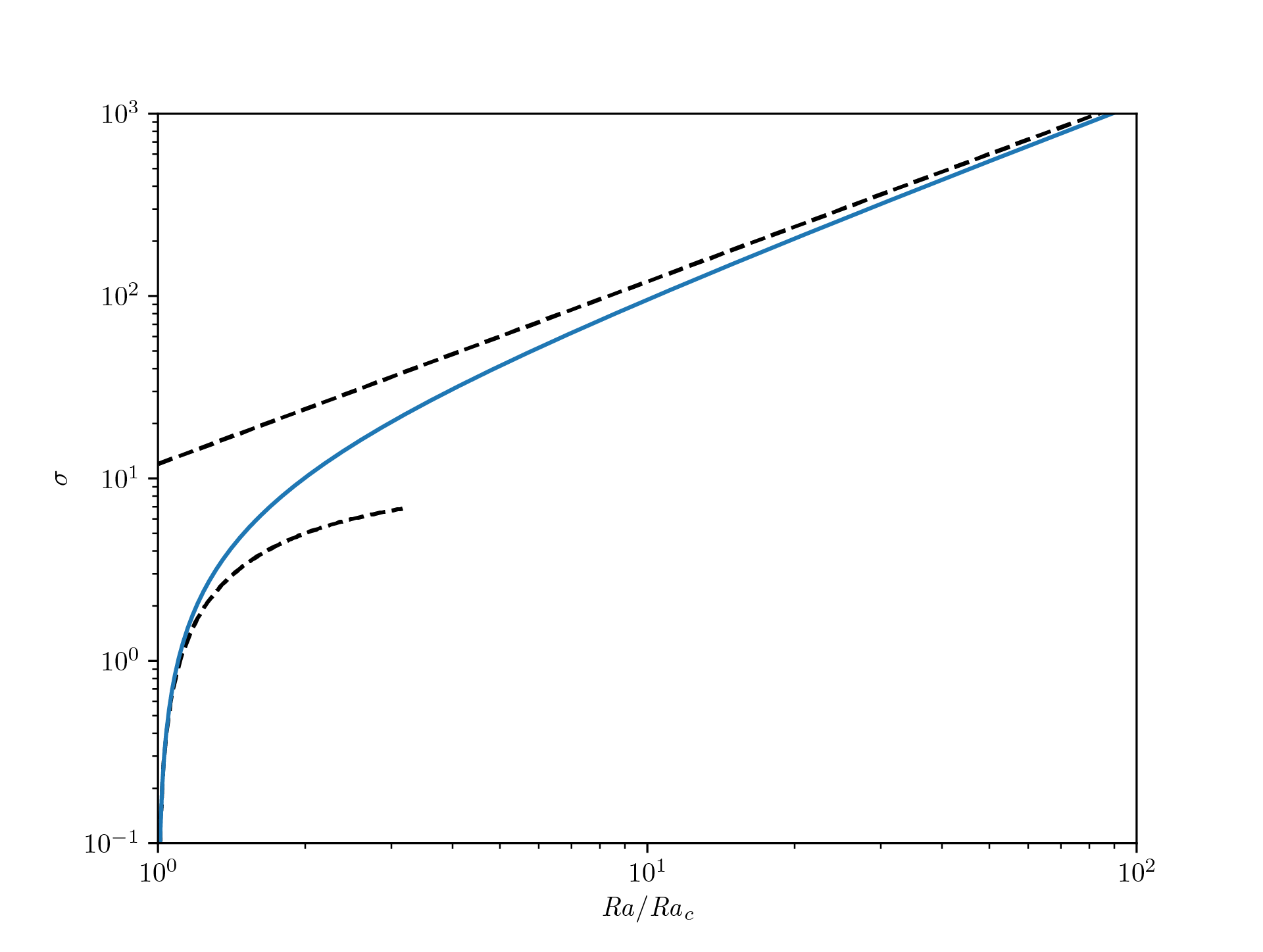
Figure 2: Instability growth rate $\sigma$ as a function of $\mbox{{Ra}}/\mbox{{Ra}}_{c}$, for infinite $Gr_{T}$, as given by the numerical solution of the full dispersion relation (solid blue line), and by the small and large $\sigma$ approximations (black dashed lines).

In the limit of a large $\sigma$,

$$2\sigma^{-1/2}\frac{\cosh\sigma^{1/2}-1}{\sinh\sigma^{1/2}}-1\rightarrow-1$$ (30)

and the dispersion relation reduces to

$$0=\frac{\sigma^{2}}{Gr_{T}}+\frac{\Phi^{+}+\Phi^{-}}{\mbox{{Ra}}}\sigma-1.$$ (31)

The positive root is

$$\sigma=\frac{\Phi^{+}+\Phi^{-}}{\mbox{{Ra}}}\frac{Gr_{T}}{2}\left[\sqrt{1+\frac{4}{Gr_{T}}\left(\frac{\mbox{{Ra}}}{\Phi^{+}+\Phi^{-}}\right)^{2}}-1\right]$$ (32)

which reduces to

$$\sigma=\frac{\mbox{{Ra}}}{\Phi^{+}+\Phi^{-}}$$ (33)

in the limit of $\frac{1}{Gr_{T}}\left(\frac{\mbox{{Ra}}}{\Phi^{+}+\Phi^{-}}\right)^{2}\ll 1$. The growth rate in the large $Gr_{T}$ limit is plotted as function of $\mbox{{Ra}}/\mbox{{Ra}}_{c}$ on figure 2.

3.2 Steady state translation

The steady state finite amplitude translation mode is solution of

$$0 =-\operatorname{D\!}p+\mbox{{Ra}}\theta,$$ (34)

$$w\operatorname{D\!}\theta =w+\operatorname{D\!}^{2}\theta.$$ (35)

Solving first the energy balance equation (35) subject to boundary conditions (6) gives

$$\theta=z+\frac{\cosh\left(\frac{w}{2}\right)-\mathrm{e}^{wz}}{2\sinh\left(\frac{w}{2}\right)}\Rightarrow T=\frac{1}{2}+\frac{\cosh\left(\frac{w}{2}\right)-\mathrm{e}^{wz}}{2\sinh\left(\frac{w}{2}\right)}.$$ (36)

Using the momentum balance equation (34) and the boundary conditions (16) then gives

$$\left(\Phi^{+}+\Phi^{-}\right)w=\mbox{{Ra}}\left[\frac{\cosh\left(\frac{w}{2}\right)}{2\sinh\left(\frac{w}{2}\right)}-\frac{1}{w}\right].$$ (37)

This transcendental equation relates the translation velocity $w$ to the Rayleigh number.

Close to onset, assuming the Péclet number, $|w|$, to be small, equation (37) can be developed as function of $(\mbox{{Ra}}-\mbox{{Ra}}_{c})/\mbox{{Ra}}_{c}$ to give to leading order

$$w=\pm 2\sqrt{15\frac{\mbox{{Ra}}-\mbox{{Ra}}_{c}}{\mbox{{Ra}}_{c}}}.$$ (38)

The corresponding temperature anomaly is

$$\theta=\frac{w}{8}\left(1-4z^{2}\right)+O(w^{2}),$$ (39)

showing that the temperature only differs from the conduction solution by an amount proportional to the Péclet number.

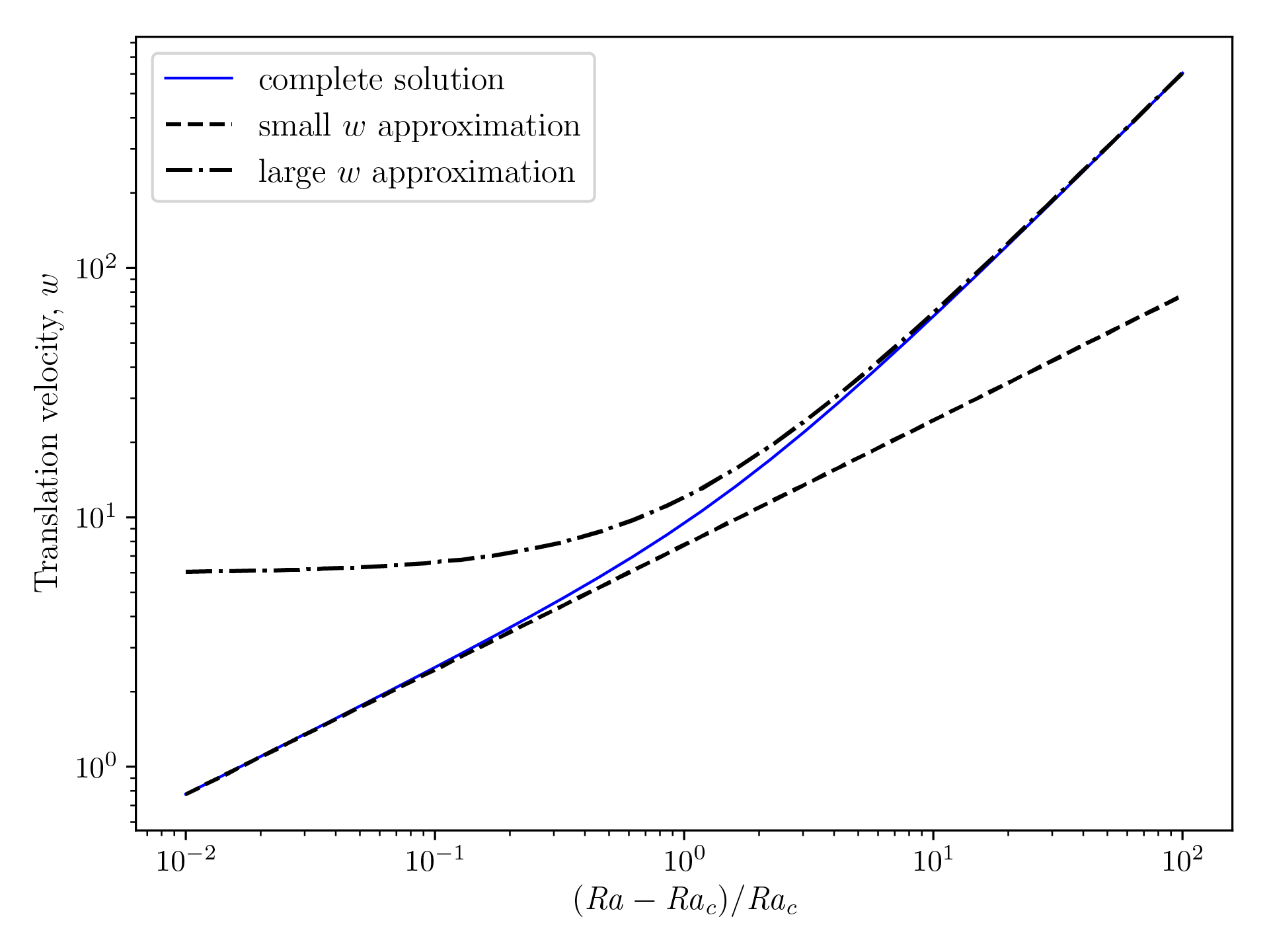
Figure 3: Finite amplitude velocity in the translation mode. The dashed line is the small velocity approximation given by eq. (38), the dash-dotted line is the large velocity approximation given by eq. (40) and the solid line is the solution to the full equation (37).

For a large Péclet number, $|w|\gg 1$, equation (37) reduces to

$$w\sim\pm\frac{\mbox{{Ra}}}{2\left(\Phi^{+}+\Phi^{-}\right)}=\pm\frac{6\mbox{{Ra}}}{\mbox{{Ra}}_{c}}.$$ (40)

Figure 3 shows how the translation velocity $|w|$ depends on Rayleigh number, computed using the full equation (37) and either the low or the large velocity development. It shows that the transition between the two regimes happens for $\mbox{{Ra}}\sim 2\mbox{{Ra}}_{c}$.

In the high Péclet number regime, the temperature anomaly takes a simple form:

$$\theta\sim z+\operatorname{sgn}(w)\left[\frac{1}{2}-\mathrm{e}^{w(z-\operatorname{sgn}(w)/2)}\right]\Rightarrow T\sim\frac{1}{2}\left[1+\operatorname{sgn}(w)\right]-\operatorname{sgn}(w)\mathrm{e}^{w(z-\operatorname{sgn}(w)/2)}.$$ (41)

The exponential in the last equation is negligible everywhere except close to the upper boundary ($z=1/2$; resp. lower boundary, $z=-1/2$) when $w\gg 1$ (resp. $w\ll-1$). Therefore, the temperature is essentially equal to that imposed at the boundary the fluid originates from ($0$ at the top, $1$ at the bottom) and adjusts to that of the opposite side in a boundary layer of thickness $\delta\sim 1/w$. In dimensional units, $\delta$ is simply defined as the thickness that makes the Péclet number around 1: $\mbox{{Pe}}=w\delta/\kappa\sim 1$. Figure 4 shows the temperature profiles for the upward and downward translation modes computed both with the exact (eq. 36) and approximate (eq. 41) expressions, showing that the approximation is quite good.

Figure 4: Temperature profile in the translation mode for $(\mbox{{Ra}}-\mbox{{Ra}}_{c})/\mbox{{Ra}}_{c}=5$. The solid (resp. dashed) line is for the ascending (resp. descending) mode calculated using the full equation (36) and the up (resp. down) triangles are obtained using the approximate equation (41).

The steady state velocity given by equation (40) can also be obtained from a simple physical argument. In the steady translation regime, the (uniform) topography at each boundary is related to the translation velocity and the phase change timescale by

$$h^{\pm}=\tau_{\phi^{\pm}}w.$$ (42)

In steady state, the excess (resp. deficit) weight of the cooler (resp. warmer) solid layer is balanced by the sum of pressure deviations from the hydrostatic equilibrium at both boundaries as

$$\alpha\rho_{0}g\frac{\Delta Td}{2}=\Delta\rho^{+}gh^{+}+\Delta\rho^{-}gh^{-},$$ (43)

where the temperature in the solid layer has been assumed uniform, i.e. the contribution of the boundary layer to its buoyancy has been neglected. This gives for the translation velocity

$$w=\frac{\alpha\rho_{0}g\Delta Td}{2(\Delta\rho^{+}g\tau_{\phi^{+}}+\Delta\rho^{-}g\tau_{\phi^{-}})}.$$ (44)

In dimensionless form, this is exactly equation (40).

It is also worth considering the heat transfer efficiency in the translation mode. Equation (35) can be integrated to show that $wT-\operatorname{D\!}{T}$ is independent of $z$ and this implies that $w=\operatorname{D\!}{T}(-\frac{1}{2})-\operatorname{D\!}{T}(\frac{1}{2})$, meaning that the difference between the conductive heat fluxes across the horizontal boundaries is equal to the advection by translation. Figure 4 show that the heat flow (Nusselt number Nu) should be computed on the exit side, where a boundary layer is produced:

$$\mbox{{Nu}}=-\operatorname{D\!}{T}\left(\operatorname{sgn}{(w)}\frac{1}{2}\right)=|w|-\operatorname{D\!}{T}\left(-\operatorname{sgn}{(w)}\frac{1}{2}\right)=|w|+\frac{w\mathrm{e}^{-|w|/2}}{2\sinh(w/2)}.$$ (45)

The small and large $|w|$ limit cases give

Nu $$=1+\frac{|w|}{2}=1+\sqrt{15\frac{\mbox{{Ra}}-\mbox{{Ra}}_{c}}{\mbox{{Ra}}_{c}}},$$ (46)

Nu $$=|w|=6\frac{\mbox{{Ra}}}{\mbox{{Ra}}_{c}},$$ (47)

respectively. The large Rayleigh number behaviour is in striking contrast to the situation encountered for standard Rayleigh-Bénard convection for which $\mbox{{Nu}}\sim\mbox{{Ra}}^{\beta}$ with $\beta\sim 1/3$.

4 Non-translating modes with $\Phi^{+}=\Phi^{-}$

In this section, we consider the situation with values of the phase change parameter of both boundaries equal, $\Phi\equiv\Phi^{+}=\Phi^{-}$.

4.1 Linear stability

Non-translating solutions can be obtained using standard approaches for the classical Rayleigh-Bénard problem. For the linear stability problem, a solution using separation of variables is sought, i.e. $u=U(z)\mathrm{e}^{\mathrm{i}kx}\mathrm{e}^{\sigma t}$ and similarly for $w$, $p$ and $\theta$. Linearized equations (18) to (20) reduce to

$$\mathrm{i}kU+DW =0,$$ (48)

$$\Pran\left[-\mathrm{i}kP+\left(\operatorname{D\!}^{2}-k^{2}\right)U\right] =\sigma U,$$ (49)

$$\Pran\left[-\operatorname{D\!}P+\left(\operatorname{D\!}^{2}-k^{2}\right)W+\mbox{{Ra}}\Theta\right] =\sigma W,$$ (50)

$$W+\left(\operatorname{D\!}^{2}-k^{2}\right)\Theta =\sigma\Theta$$ (51)

since, at the linear stage, the problem is fully degenerate in terms of orientation of the mode which can be taken as depending only on $x$. These equations must be complemented by boundary conditions applying at $z=\pm\frac{1}{2}$:

$$\operatorname{D\!}U+\mathrm{i}kW =0,$$ (52)

$$\pm\Phi^{\pm}W+2\operatorname{D\!}W-P =0,$$ (53)

$$\Theta =0.$$ (54)

This forms a generalized eigenvalue problem that we solve using a Chebyshev-collocation pseudo-spectral approach (e.g. Canuto et al., 1988; Guo et al., 2012). Given the Chebyshev-Gauss-Lobatto nodal point $z_{i}=\cos\frac{i\upi}{N},i=0...N$, in the interval $\left[-1,1\right]$, the values of the $z$-dependent mode functions at $z_{i}/2$ is noted as $U_{i}$ for U and similarly for other variables. Division by $2$ is required here to map the interval on which Chebyshev polynomials are defined onto $\left[-\frac{1}{2},\frac{1}{2}\right]$. The $k^{th}$ derivative of each function at the nodal points is related to the nodal values of the function itself by differentiation matrices:

$${\bm{U}}^{(k)}=\mathsfbi{D}^{(k)}\cdot{\bm{U}}.$$ (55)

The calculation of the differentiation matrices is done using a python adaptation of DMSUITE (Weideman & Reddy, 2000). With these differentiation matrices, the system of equations (48) to (51) can be written as a generalized eigenvalue problem of the form

$$\mathsfbi{L}\cdot{\bm{X}}=\sigma\mathsfbi{R}\cdot{\bm{X}}$$ (56)

with ${\bm{X}}=({\bm{P}};{\bm{U}};{\bm{W}};{\bm{\Theta}})^{T}$ the global vertical mode vector composed of the concatenation of vectors $P_{i}$, $U_{i}$, $W_{i}$ and $\Theta_{i}$, and $\mathsfbi{L}$ and $\mathsfbi{R}$ two matrices representing the system with its boundary conditions. The general structure of $\mathsfbi{L}$ reads as

$$\mathsfbi{L}=\blockarray{ccccc}0\mathrel{\mathop{\mathchar 58\relax}}N&0\mathrel{\mathop{\mathchar 58\relax}}N0\mathrel{\mathop{\mathchar 58\relax}}N1\mathrel{\mathop{\mathchar 58\relax}}N-1\\ \block{(cccc)l}\mathsfbi{0}\mathrm{i}k\mathsfbi{I}\mathsfbi{D}\mathsfbi{0}\ 0\mathrel{\mathop{\mathchar 58\relax}}N\\ \mathsfbi{0}\mathsfbi{D}\mathrm{i}k\mathsfbi{I}\mathsfbi{0}\ 0\\ -\Pran\mathrm{i}k\mathsfbi{I}\Pran\left(\mathsfbi{D}^{(2)}-k^{2}\mathsfbi{I}\right)\mathsfbi{0}\mathsfbi{0}\ 1\mathrel{\mathop{\mathchar 58\relax}}N-1\\ \mathsfbi{0}\mathsfbi{D}\mathrm{i}k\mathsfbi{I}\mathsfbi{0}\ N\\ -\mathsfbi{I}\mathsfbi{0}\Phi^{+}\mathsfbi{I}+2\mathsfbi{D}\mathsfbi{0}\ 0\\ -\Pran\mathsfbi{D}\mathsfbi{0}\Pran\left(\mathsfbi{D}^{(2)}-k^{2}\mathsfbi{I}\right)\Pran\mbox{{Ra}}\mathsfbi{I}\ 1\mathrel{\mathop{\mathchar 58\relax}}N-1\\ -\mathsfbi{I}\mathsfbi{0}-\Phi^{-}\mathsfbi{I}+2\mathsfbi{D}\mathsfbi{0}\ N\\ \mathsfbi{0}\mathsfbi{0}\mathsfbi{I}\left(\mathsfbi{D}^{(2)}-k^{2}\mathsfbi{I}\right)\ 1\mathrel{\mathop{\mathchar 58\relax}}N-1\\$$ (57)

with $\mathsfbi{I}$ and $\mathsfbi{0}$ the identity and zero matrices, respectively. The restrictions of line and column indices, indicated on the right and top of the matrix respectively, are necessary to leave out the boundary points from applications of equations (48) to (51) since these follow equations (52)-(54) instead. For example, in the second line of the matrix that represents equation (52), only the first line (index $0$) of the matrice $\mathsfbi{0},\mathsfbi{D},\mathrm{i}k\mathsfbi{I}$ and $\mathsfbi{0}$ are present. Note that the boundary values for the temperature are simply left out since the Dirichlet boundary condition (54) is, in a collocation approach, naturally enforced by removing the extreme Chebyshev points.

The $\mathsfbi{R}$ matrix contains ones on the diagonal corresponding to the interior points of the equations for ${\bm{U}}$, ${\bm{W}}$ and ${\bm{\Theta}}$ and zeros elsewhere. When solving for an infinite Prandtl number, which is the case below, the interior points for the ${\bm{U}}$ and ${\bm{W}}$ equations are also set to 0, leaving ones only for the interior points of the ${\bm{\Theta}}$ equation. The resulting system is singular and many eigenvalues are infinite, one for each zero in the $\mathsfbi{R}$ matrix. Filtering these spurious eigenvalues leaves us with the relevant eigenvalues that are used to assess stability. For any values of $\Phi^{-}$, $\Phi^{+}$ and $k$, the minimum value of Ra that makes the real part of one of the eigenvalues become positive is the critical Rayleigh number for perturbations with that wavenumber. Minimizing Ra as function of $k$ gives the critical Rayleigh number for all infinitesimal perturbations.

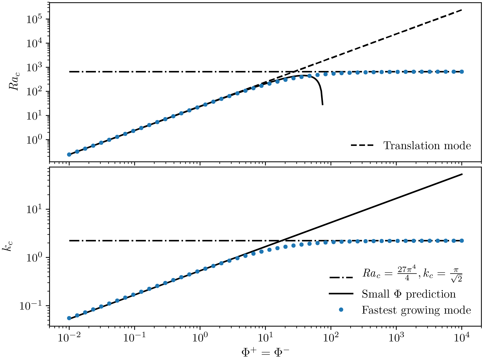
Figure 5: Critical Rayleigh number (top) and wavenumber (bottom) as function of the phase change numbers, both taken equal here. Filled circles are results of the calculation using the Chebyshev-collocation technique, the dash-dotted lines represent the classical $\Phi\rightarrow\infty$ limit, the dashed line in the upper panel represents the result for the translating mode (eq. 23) and the solid lines represent the small $\Phi$ leading order development.

Figure 5 shows the evolution of the critical Rayleigh number and the associated wavenumber as function of the value of $\Phi^{\pm}$, both taken equal, $\Phi^{+}=\Phi^{-}=\Phi$. One can see that the classical value derived by Rayleigh (1916) is recovered when $\Phi\rightarrow\infty$, as expected. In the other limit, $\Phi\rightarrow 0$, the critical Rayleigh number follows the analytical expression obtained for the translation mode (§ 3) while $k\rightarrow 0$, as expected.

The behaviour of the system in the limit of small $\Phi$ can be obtained using a polynomial expansion of all the functions, both in $z$ and $\Phi$. Specifically, considering the symmetry of the problem around $z=0$, we write the temperature as

$$\Theta=\sum_{n=0}^{N}a_{n}z^{2n}.$$ (58)

The Hermitian character of the linear problem (see appendix A) ensures that $\sigma$ is real and, therefore, $\sigma=0$ at onset. Then $W$ and $U$ can be obtained using equations (51) and (48). Equations (49) and (50) then provide two expressions for $DP$ and their equality implies several equations, one for each polynomial order considered. All the functions are developed to the same order as the temperature, $2N$. Note that even if the definition of $\Theta$ for a given $N$ only requires $N+1$ coefficients $a_{n}$, the development of the other profiles to the same order requires the inclusion of $a_{n}$ for values up to $n=N+2$ because of the derivatives in the linear system. Using, for example, $N=2$ gives a pressure gradient $DP$ that contains terms in $z^{2n},n=0..2$, and provides therefore three independent equations for the equality between the two expressions. With the symmetry considered here, the boundary conditions (52)– (54) bring three additional equations for the coefficients $a_{n}$.

Setting first $\Phi=0$ leads to a non trivial solution only for $\mbox{{Ra}}=0$ and $k=0$, the solution being equal to the low $\Phi$ development of the translation solution. To go beyond that, each coefficient $a_{n}$ is itself developed as a polynomial of $\Phi$:

$$a_{n}=\sum_{j=0}^{J}a_{n,j}\Phi^{j}.$$ (59)

Similarly, the critical Rayleigh number $\mbox{{Ra}}_{c}$ and the square of the critical wavenumber $k^{2}$ are developed in powers of $\Phi$:

$$\mbox{{Ra}}_{c}=\sum_{j=0}^{J}r_{j}\Phi^{j},\qquad k_{c}^{2}=\sum_{j=0}^{J}K_{j}\Phi^{j}.$$ (60)

The three boundary conditions and the equations implied by the equality of the two pressure expressions are then written and solved for increasing degrees in the development in $\Phi$. In practice, we restrict ourselves to $N=J=2$. At order 0 in $\Phi$, the set of linear equations can admit a non-trivial solution only if the determinant of the implied matrix is zero, which provides two possible values of $r_{0}$. The lowest one admits a minimum, $r_{0}=0$, for $K_{0}=0$. This implies $a_{2,0}=a_{3,0}=a_{4,0}=0$ and $a_{1,0}=-4a_{0,0}$. At order 1 in $\Phi$, we get directly that $a_{2,1}=a_{3,1}=a_{4,1}=0$, $a_{1,1}=-4a_{0,1}$ and $r_{1}=24$ with no information on $K_{1}$. This is however obtained at the next order where we find that $K_{1}=9/32$ minimizes $r_{2}$, which is then $r_{2}=-81/256$. The order 2 coefficients are also obtained as a function of $a_{0,0}$, which is the value of the maximum of $\Theta$. These can then be used to determine the shape of the different function $\Theta$, $W$, $U$ and $P$ for small values of $\Phi$. To leading order in $\Phi$ we get

$$k_{c} =\frac{3}{4\sqrt{2}}\sqrt{\Phi}$$ (61)

$$\mbox{{Ra}}_{c} =24\Phi-\frac{81}{256}\Phi^{2},$$ (62)

$$\Theta =(1-4z^{2})\Theta_{max},$$ (63)

$$W =8\Theta_{max},$$ (64)

$$U =-3\mathrm{i}\sqrt{2\Phi}z\Theta_{max},$$ (65)

$$P =\frac{z}{2}\left(39-64z^{2}\right)\Phi\Theta_{max}.$$ (66)

Figure 6: Variation of the maxima of profiles of $P$, $U$ and $W$ of the first unstable mode, that for $\Theta$ being set to 1, as a function of $\Phi$. The bottom panel shows the difference between $24\Phi$ and the critical Rayleigh number. On each plot, the solid circles are the results of the calculation using the Chebyshev-collocation method while the dashed lines are the low $\Phi$ predictions of equations (62) to (66).

$\Theta_{max}=a_{0,0}$ is used to normalise all profiles. Note that the shape of the temperature (eq. 63) and vertical velocity (eq. 64) profiles are of order 0 in $\Phi$ and are equal to their counterpart in the steady-state translation solution (eq. 39). The small $\Phi$ development of the solution to the linear problem can be compared to the results obtained using the Chebyshev-collocation method for cross-validation. The match between the mode profiles is very good for $\Phi\leq 0.1$. Figure 5 shows the variation of $\mbox{{Ra}}_{c}$ and $k_{c}$ as function of $\Phi$ as computed by the Chebyshev-collocation approach (in solid symbols) as well as the analytical value classically obtained for non-penetrating conditions and the small $\Phi$ expansion. Additionally, figure 6 shows the variation of the maximum of profiles of $P$, $U$ and $W$, that of $\Theta$ being set to 1, as well as the difference between the critical Rayleigh number for uniform translation ($24\Phi$) and that for a deforming mode, each as function of $\Phi$. It shows the consistency between the calculations using the Chebyshev-collocation approach and the low $\Phi$ development.

At low $\Phi$, the wavelength of the first unstable mode tends to infinity as $\sim 1/\sqrt{\Phi}$, which means that deformation of the solid becomes negligible. Accordingly, the viscous stress ceases to be a limiting factor for the flow and $Ra_{c}/\Phi$, which contains no viscosity, tends to a constant value. This ratio,

$$\frac{\mbox{{Ra}}}{\Phi}=\frac{\rho\alpha\Delta Td^{2}}{\Delta\rho^{\pm}\kappa\tau_{\phi}}\equiv\frac{\Delta\rho_{T}}{\Delta\rho^{\pm}}\frac{\tau_{\kappa}}{\tau_{\phi}},$$ (67)

is the ratio of the driving thermal density difference $\Delta\rho_{T}$ to that involved in the phase change, times the ratio of the thermal timescale to the phase change one, and can be considered as the effective Rayleigh number in the low $\Phi$ limit.

Figure 7 shows the first unstable mode for different values of the phase change parameter. In the case of $\Phi=10^{5}$, the critical Rayleigh number and wavenumber are very close to that obtained using classical non-penetrating boundary conditions (fig. 5) and so is the first unstable mode. For $\Phi=10$, the critical Rayleigh number has already decreased significantly ($\mbox{{Ra}}_{c}=190$), the critical wavelength significantly increased ($\lambda_{c}=4.55$) and the critical mode displays streamlines that cross both boundaries. For $\Phi=10^{-2}$, the critical Rayleigh number is a bit less than $0.24$, the critical wavelength is about $115$ and streamlines are essentially vertical. At each horizontal position, this mode of convection has exactly the same shape as the linearly unstable translation mode but it is modulated laterally, with a very long wavelength that increases as $\sim 1/\sqrt{\Phi}$ when $\Phi\rightarrow 0$. The fact that this makes the critical Rayleigh number smaller than that for pure solid-body translation is rather mysterious.

Figure 7: First unstable mode for three different values of $\Phi^{+}=\Phi^{-}$: $10^{5}$ (top), $10$ (middle) and $10^{-2}$ (bottom). The color represents temperature and the flow lines thickness is proportional to the norm of the velocity. Note that for the bottom panel the axis are scaled differently owing to the large wavelength of the mode.

The critical Rayleigh number for the instability for the non-null $k$ mode is always lower than that for pure translation, as shown by Eq. (62) and fig. 5 and should therefore always be favored. This might be true in an infinite layer but, in practical cases, the horizontal direction is periodic, either in numerical models or in a planetary mantle. In that case, the minimal value of $k$ that can be attained is $2\upi/L$ with $L$ the horizontal periodicity. If the value of $k$ corresponding to the critical Rayleigh number is smaller than $2\upi/L$, the translation mode could still be favored.

Figure 8: Growth rate of deforming perturbation over a steady translating solution as function of the perturbation wavenumber $k$, for different values of the reduced Rayleigh number $\varepsilon=(\mbox{{Ra}}-\mbox{{Ra}}_{c})/\mbox{{Ra}}_{c}$ and for $\Phi^{+}=\Phi^{-}=1$.

The study of the stability of the uniformly translating solution with respect to laterally varying modes is a simple extension to the stability of the conduction solution. Considering now that $(p,{\bm{v}},\theta)$ are infinitesimal perturbations with respect to the steady translation solution $(p_{t},w_{t}\hat{{\bm{z}}},T_{t})$, the only equation to be modified compared to that treated in section 4.1 at infinite Prandtl number is the temperature equation that now reads

$$\left(\operatorname{D\!}^{2}-k^{2}\right)\Theta-w_{t}\operatorname{D\!}{\Theta}-W\operatorname{D\!}{T_{t}}=\sigma\Theta$$ (68)

instead of equation (51). Using the steady translation solution provided in section 3.2, this equation can be implemented in the stability calculation to compute the growth rate of a deforming perturbation of wavenumber $k$ when a steady translation solution is in place for a given Rayleigh number above the critical value for the translation solution. We denote by $\varepsilon=(\mbox{{Ra}}-\mbox{{Ra}}_{c})/\mbox{{Ra}}_{c}$ the reduced Rayleigh number, $\mbox{{Ra}}_{c}=12(\Phi^{+}+\Phi^{-})$ being here the critical value for the onset of uniform translation. When $\varepsilon$ tends to zero, the translation velocity $w_{t}$ tends to zero and the system of equations tends to that solved for the stability of the steady conduction solution. But since $\varepsilon=0$ corresponds to the critical Rayleigh number for the translation solution that is finitely greater than the critical value for the instability with finite $k$, we expect a finite instability growth rate in a finite band of wave numbers. We therefore expect an infinitely slow translation solution to be unstable with respect to deforming modes. However, when the Rayleigh number is increased above the critical value for the translation mode, we expect this translation mode with a finite velocity to become more stable since perturbations with a finite $k$ are then transported away by translation. Figure 8 indeed shows that, for a given value of the phase change number $\Phi$ (equal for both boundaries here), increasing the Rayleigh number above the critical value for the translation mode, and therefore the steady state translation velocity, the linear growth rate of the deforming mode decreases. For a given Rayleigh number, the growth rate curve as function of wave number displays a maximum and this maximum decreases with Rayleigh number and eventually becomes negative. There is therefore a maximum Rayleigh number beyond which the translation solution is linearly stable against any deforming perturbation. Figure 9 shows the range of unstable modes in the $k-\varepsilon$ space for three different values of the phase change number. The range of Rayleigh numbers above the critical one for translation that allows the finite $k$ instabilities to develop shrinks when $\Phi$ decreases and the translation mode becomes increasingly more relevant. Figure 10 shows that the maximum growth rate of the instability at $\varepsilon=0$ varies linearly with $\Phi$ and so does the maximum value of $\varepsilon$ for an instability to develop. The wave number for the instability is found to be equal to that for the instability of the conductive solution (fig. 9) and therefore varies as $\sqrt{\Phi}$ (fig. 5).

Figure 9: Range of wave numbers as function of the reduced Rayleigh number for which the translation solution is unstable versus deforming modes. Three different shaded regions for three different values of $\Phi$ are represented. For each shaded area, the dashed line represents the values of the wave number giving the maximum growth rate as function of the reduced Rayleigh number.

Figure 10: Maximum growth rate for a non-null $k$ mode at the critical Rayleigh number for the onset of the translation mode (top) and maximum reduced Rayleigh number for a positive growth rate of a deforming instability over a finite amplitude translation mode (bottom), as function of the phase change number.

4.2 Weakly non-linear analysis

Going beyond the linear stability is necessary to assess the behaviour of the system at Rayleigh numbers larger than the critical value, in particular to investigate the heat transfer efficiency of the convective system. We here follow the approach classically developed for weakly nonlinear dynamics (Malkus & Veronis, 1958; Schlüter et al., 1965; Manneville, 2004). The system of partial differential equations (18)- (20) is separated into its linear and nonlinear parts as

$$\mathbf{L}(\partial_{t},\partial_{x},\partial_{z},\mbox{{Ra}})\mathbf{X}=\mathbf{N}(\mathbf{X},\mathbf{X}),$$ (69)

with $\mathbf{X}=(p;u;w;\theta)^{T}$ and for an infinite Prandtl case

$$\mathbf{L}=\left(\begin{array}[]{cccc}0&\partial_{x}&\partial_{z}&0\\ -\partial_{x}&\nabla^{2}&0&0\\ -\partial_{z}&0&\nabla^{2}&\mbox{{Ra}}\\ 0&0&1&\nabla^{2}-\partial_{t}\end{array}\right),\quad\mathbf{N}(\mathbf{X}_{l},\mathbf{X}_{m})=\left[\begin{array}[]{c}0\\ 0\\ 0\\ u_{l}\partial_{x}\theta_{m}+w_{l}\partial_{z}\theta_{m}\end{array}\right].$$ (70)

The linear operator is further developed around the critical Rayleigh number as

$$\mathbf{L}=\mathbf{L}_{c}-(\mbox{{Ra}}-\mbox{{Ra}}_{c})\mathbf{M}.$$ (71)

By giving $\mbox{{Ra}}_{c}$ as weight to the $\theta$ part in the dot product $\braket{\bullet}{\bullet}$, it can be shown that the operator $\mathbf{L}_{c}$ is self-adjoint (Hermitian), $\braket{\mathbf{X}_{2}}{\mathbf{L}\mathbf{X}_{1}}=\braket{\mathbf{L}\mathbf{X}_{2}}{\mathbf{X}_{1}}$ (see appendix for details). Among other things, it implies that all its eigenvalues are real and the marginal state is characterized by $\partial_{t}=0$. The solution $\mathbf{X}$ and the Rayleigh number are developed as

$$\mathbf{X} =\epsilon\mathbf{X}_{1}+\epsilon^{2}\mathbf{X}_{2}+\epsilon^{3}\mathbf{X}_{3}+...$$ (72)

Ra $$=\mbox{{Ra}}_{c}+\epsilon\mbox{{Ra}}_{1}+\epsilon^{2}\mbox{{Ra}}_{2}+...$$ (73)

and equation (69) leads to a set of equations for the increasing order of $\epsilon$:

$$\mathbf{L}_{c}\mathbf{X}_{1} =\mathbf{0},$$ (74)

$$\mathbf{L}_{c}\mathbf{X}_{2} =\mathbf{N}(\mathbf{X}_{1},\mathbf{X}_{1})+\mbox{{Ra}}_{1}\mathbf{M}\mathbf{X}_{1},$$ (75)

$$\mathbf{L}_{c}\mathbf{X}_{3} =\mathbf{N}(\mathbf{X}_{1},\mathbf{X}_{2})+\mathbf{N}(\mathbf{X}_{2},\mathbf{X}_{1})+\mbox{{Ra}}_{1}\mathbf{M}\mathbf{X}_{2}+\mbox{{Ra}}_{2}\mathbf{M}\mathbf{X}_{1},$$ (76)

$$\mathbf{L}_{c}\mathbf{X}_{n} =\sum_{l=1}^{n-1}\mathbf{N}(\mathbf{X}_{l},\mathbf{X}_{n-l})+\sum_{l=1}^{n-1}\mbox{{Ra}}_{l}\mathbf{M}\mathbf{X}_{n-l}.$$ (77)

Equation (74) is simply that of the linear stability problem and its solution is $\mathbf{X}_{1}=\mathbf{X}_{c}$ which can be suitably normalised such that the maximum value of W is 1. Taking the scalar product of equations of subsequent orders by $\mathbf{X}_{1}$ and making use of the Hermitian properties of $\mathbf{L}_{c}$ provides solvability conditions (Fredholm alternative) that determine the values of $\mbox{{Ra}}_{i}$. For $\mbox{{Ra}}_{1}$ one gets:

$$\mbox{{Ra}}_{1}=-\frac{\braket{\mathbf{X}_{1}}{\mathbf{N}(\mathbf{X}_{1},\mathbf{X}_{1})}}{\braket{\mathbf{X}_{1}}{\mathbf{M}\mathbf{X}_{1}}}.$$ (78)

The $x$ dependence of $\mathbf{X}_{1}$ is of the form $\mathrm{e}^{\mathrm{i}k_{c}x}$, i.e.

$$\mathbf{X}_{1}=\mathbf{Z}_{1,1}(z)\mathrm{e}^{\mathrm{i}k_{c}x}+c.c.,$$ (79)

with $\mathbf{Z}_{1,1}(z)=(P_{1,1}(z);U_{1,1}(z);W_{1,1}(z);\Theta_{1,1}(z))^{T}$ the vector composed of the four vertical modes for all four variables, at degree 1 of weakly non-linear development (first index) and first mode in the horizontal direction (second index).

Then, $\mathbf{N}(\mathbf{X}_{1},\mathbf{X}_{1})$ contains two contributions to its $x$ dependence, one constant and one in $\mathrm{e}^{\mathrm{i}2k_{c}x}$. It is therefore orthogonal to $\mathbf{X}_{1}$ and it can then be concluded that $\mbox{{Ra}}_{1}=0$. The general solution to equation (75) is the sum of the solution to the homogeneous equation and a particular solution of the equation with a right-hand-side. Since we are seeking a solution $\mathbf{X}_{2}$ which adds to $\mathbf{X}_{1}$, i.e. orthogonal to it, and since $\mathbf{X}_{1}$ is the general solution to the homogeneous equation, only the particular solution is of interest. The $x$ dependence of $\mathbf{X}_{2}$ will contain a constant value of the form $\mathbf{Z}_{2,0}(z)$ and a term of the form $\mathbf{Z}_{2,2}(z)\mathrm{e}^{\mathrm{i}2k_{c}x}$. Computing the scalar product of equation (76) by ${\mathbf{X}}_{1}$ gives the value of $\mbox{{Ra}}_{2}$:

$$\mbox{{Ra}}_{2}=-\frac{\braket{\mathbf{X}_{1}}{\mathbf{N}(\mathbf{X}_{2},\mathbf{X}_{1})}+\braket{\mathbf{X}_{1}}{\mathbf{N}(\mathbf{X}_{1},\mathbf{X}_{2})}}{\braket{\mathbf{X}_{1}}{\mathbf{M}\mathbf{X}_{1}}}.$$ (80)

$\mathbf{X_{2}}$ containing a term proportional to $\mathrm{e}^{i2k_{c}x}$ and a term independent of $x$, $\mathbf{N}(\mathbf{X}_{2},\mathbf{X}_{1})$ and $\mathbf{N}(\mathbf{X}_{1},\mathbf{X}_{2})$ have contributions of the form $\mathrm{e}^{\pm ik_{c}x}$ which can resonate with $\mathbf{X}_{1}$ and make $\mbox{{Ra}}_{2}$ non-null. In that case, the amplitude parameter is, to leading order,

$$\epsilon=\sqrt{\frac{\mbox{{Ra}}-\mbox{{Ra}}_{c}}{\mbox{{Ra}}_{2}}}.$$ (81)

The procedure can be extended to any higher order and the general behaviour can be predicted by recursive reasoning. In particular, it is easy to show that solutions of even and odd order contain contributions to their $x$ dependence as even and odd powers of $\mathrm{e}^{\mathrm{i}k_{c}x}$ up to their order value, i.e.

$$\mathbf{X}_{2n} =\sum_{l=0}^{n}\mathbf{Z}_{2n,2l}(z)\mathrm{e}^{\mathrm{i}2lk_{c}x}+c.c.,$$ (82)

$$\mathbf{X}_{2n+1} =\sum_{l=0}^{n}\mathbf{Z}_{2n+1,2l+1}(z)\mathrm{e}^{\mathrm{i}(2l+1)k_{c}x}+c.c.,$$ (83)

the vertical normal mode $\mathbf{Z}_{n,l}=(P_{n,l}(z);U_{n,l}(z);W_{n,l}(z);\Theta_{n,l}(z))^{T}$ being indexed with the order $n$ of the solution and harmonic number $l$ in the $x$ dependence. It also appears recursively that

$$\mbox{{Ra}}_{2n} =-\frac{\sum_{l=1}^{2n}\braket{\mathbf{X}_{1}}{\mathbf{N}(\mathbf{X}_{l},\mathbf{X}_{2n+1-l})}+\sum_{l=1}^{n-1}\mbox{{Ra}}_{2l}\braket{\mathbf{X}_{1}}{\mathbf{M}\mathbf{X}_{2(n-l)+1}}}{\braket{\mathbf{X}_{1}}{\mathbf{M}\mathbf{X}_{1}}},$$ (84)

$$\mbox{{Ra}}_{2n+1} =0.$$ (85)

This is true for orders 1 and 2, as explained above and, assuming it holds up to degrees $2n-1$ and $2n$, the expressions for degrees $2n+1$ and $2n+2$ can be predicted from equation (77). First, equation (77) of order $2n+1$ includes on the right-hand-side only terms up to degree $2n$ and can be used to predict the form of $\mathbf{X}_{2n+1}$. Each term of the form $\mathbf{N}(\mathbf{X}_{l},\mathbf{X}_{2n+1-l})$ contains only odd powers of $\mathrm{e}^{\mathrm{i}k_{c}x}$ since it is composed of products of even (resp. odd) and odd (resp. even) polynomials of $\mathrm{e}^{\mathrm{i}k_{c}x}$ for $l$ even (resp. odd). Each term of the form $\mbox{{Ra}}_{l}\mathbf{M}\mathbf{X}_{2n+1-l}$ is either null for $l$ odd or an odd polynomial of $\mathrm{e}^{\mathrm{i}k_{c}x}$ for $l$ even. Summing up, the right-hand-side of the equation being an odd polynomial of $\mathrm{e}^{\mathrm{i}k_{c}x}$, the solution to the equation is of the form (83).

Taking the dot product of equation (77) of order $2n+2$ by $\mathbf{X}_{1}$ and using the Hermitian character of $\mathbf{L}_{c}$ provides the equation for $\mbox{{Ra}}_{2n+1}$. Starting first with the last term on the right-hand-side, all the terms in the sum except the one in $\mbox{{Ra}}_{2n+1}$ drop out either because $\mbox{{Ra}}_{l}$ is null for $l$ odd or because the dot product $\braket{\mathbf{X}_{1}}{\mathbf{M}\mathbf{X}_{2n+2-l}}=0$ for $l$ even since $\mathbf{X}_{2n+2-l}$ then contains only even powers of $\mathrm{e}^{\mathrm{i}k_{c}x}$. We are left with $\mbox{{Ra}}_{2n+1}\braket{\mathbf{X}_{1}}{\mathbf{M}\mathbf{X}_{1}}$. Considering the first sum on the right-hand-side, each term $\mathbf{N}(\mathbf{X}_{l},\mathbf{X}_{2n+2-l})$ is an even polynomial of $\mathrm{e}^{\mathrm{i}k_{c}x}$, as the product of either two even polynomials (for $l$ even) or two odd polynomials (for $l$ odd). Therefore, each of these terms is orthogonal to $\mathbf{X}_{1}$ and $\mbox{{Ra}}_{2n+1}=0$. The same equation (77)_2n+2 contains only even powers of $\mathrm{e}^{\mathrm{i}k_{c}x}$ on the right-hand-side and this justifies equation (82) for the order $2n+2$.

Finally, equation (84)_2n+2 is obtained by simply taking the dot product of equation (77)_2n+3 by $\mathbf{X}_{1}$.

An important diagnostic for convection is the heat transfer efficiency measured by the dimensionless mean heat flux density, the Nusselt number Nu. Since the temperature is uniform on each horizontal boundary and the average vertical velocity is null for the deforming mode considered here, the advective heat transfer across the horizontal boundaries is null. Therefore, the Nusselt number can easily be computed by taking the vertical derivative of the temperature at either boundary. In the Fourier decomposition used for the non-linear analysis, only the zeroth order term in $\mathrm{e}^{\mathrm{i}k_{c}x}$ contribute to the horizontal average and they only appear in terms that are even in the $\epsilon$ development. Restricting ourselves here to an order 2 development, the Nusselt number can be computed as

$$\mbox{{Nu}}=1-\epsilon^{2}D\theta_{2,0}\left(\frac{1}{2}\right)=1-D\theta_{2,0}\left(\frac{1}{2}\right)\frac{\mbox{{Ra}}_{c}}{\mbox{{Ra}}_{2}}\frac{\mbox{{Ra}}-\mbox{{Ra}}_{c}}{\mbox{{Ra}}_{c}}$$ (86)

where equation (81) was used. This equation shows the classical result that the convective heat flow, $\mbox{{Nu}}-1$, increases linearly with the reduced Rayleigh number $\varepsilon=(\mbox{{Ra}}-\mbox{{Ra}}_{c})/\mbox{{Ra}}_{c}$ for small values of $\varepsilon$ and the determination of the coefficient of proportionality, $A$, is the main goal of the weakly non-linear analysis presented here. Note that $\mathbf{N}(\mathbf{X}_{2},\mathbf{X}_{1})$ and $\mathbf{N}(\mathbf{X}_{1},\mathbf{X}_{2})$ only have a non-zero component only along the $\theta$ space (eq. 70) so that, because of our definition of the dot product (§ A) and using equation (80), $\mbox{{Ra}}_{2}$ is proportional to $\mbox{{Ra}}_{c}$.

The procedure just outlined can be applied to the case with classical boundary conditions. In particular, for free-slip non-penetrating boundary conditions, the problem can be solved analytically (Malkus & Veronis, 1958; Manneville, 2004). Starting with the vertical velocity in the critical mode as $w_{1}=\sin kx\cos\pi z$, one gets $\theta_{1}=\left(\pi^{2}+k^{2}\right)^{-1}\sin kx\cos\pi z$, $\mbox{{Ra}}_{c}=\left(\pi^{2}+k^{2}\right)^{3}/k^{2}$, $w_{2}=0$, $\theta_{2}=\left(8\pi\left(\pi^{2}+k^{2}\right)\right)^{-1}\sin 2\pi z$ and $\mbox{{Ra}}_{2}=\left(\pi^{2}+k^{2}\right)^{2}/8k^{2}$. This gives $A=-D\theta_{2,0}\left(1/2\right)\mbox{{Ra}}_{c}/\mbox{{Ra}}_{2}=2$.

Figure 11: Heat flux coefficient as a function of the phase change numbers, equal to each other (left), and Nusselt number as a function of Rayleigh number for different values of $\Phi^{\pm}$ (right). The solid line gives the limit of two non-penetrating boundaries while the dashed line represents the first order development obtained for $\Phi\rightarrow 0$ (eq. 91).

Similarly, the low $\Phi$ expansion of the linear mode, equations (61)– (66), can be used to compute the behaviour of coefficient $A$ at low $\Phi$ values. We choose $\Theta_{max}=1/16$ to have a normalisation consistent with the one above and the solution at order 2 is searched in the form of $z$ polynomials, and we get, to order 1 in $\Phi$,

$$\theta_{2} =-\frac{z}{48}\left(z^{2}-\frac{1}{4}\right)\left[1+\left(1-\frac{\Phi}{64}\right)\cos{2k_{c}x}\right],$$ (87)

$$u_{2} =-\frac{\sqrt{\Phi}}{192\sqrt{2}}\sin{2k_{c}x},$$ (88)

$$w_{2} =\frac{z\Phi}{256}\cos{2k_{c}x},$$ (89)

$$\mbox{{Ra}}_{2} =\frac{1}{320}-\frac{43\Phi}{430080}.$$ (90)

The heat flux coefficient is then, to order 1 in $\Phi$:

$$A=\frac{4480}{1344-43\Phi}.$$ (91)

Figure 11 represents the value of the heat flux coefficient $A$ as function of $\Phi$ obtained using the Chebyshev-collocation approach described above (solid circles, see appendix B for details on the calculation of non-linear terms) and the two limiting cases of $\Phi\rightarrow\infty$ (solid line) and $\Phi\rightarrow 0$ (dashed line), which shows a good match.

The heat flux coefficient $A$, which equals 2 for classical non-penetrating boundaries, tends to $10/3$ when $\Phi\rightarrow 0$. This $\sim 50\%$ increase makes the Nusselt number increase when $\Phi$ tends to zero but the main effect comes from the decrease of the critical Rayleigh number as $\sim 24\Phi$, which makes the slope $\operatorname{d\!}{\mbox{{Nu}}}/\operatorname{d\!}{\mbox{{Ra}}}$ go to infinity as $\sim 5/36\Phi$. This is illustrated on figure 11 which shows the $\mbox{{Nu}}-\mbox{{Ra}}$ relationship derived from this analysis for different values of $\Phi$. The heat transfer efficiency is greatly increased by decreasing $\Phi$ for two reasons. Firstly, it makes the critical Rayleigh number decrease so that convection starts with a lower Rayleigh number. Secondly, the rate at which the Nusselt number increases with Ra above its critical value is also drastically increased when $\Phi$ is decreased.

5 Solutions with only one phase change boundary

Let us now consider the case when only one boundary is a liquid-solid phase change, the other one being subject to a non-penetrating condition. With the plane layer geometry considered here, the situation with the upper boundary a phase change is symmetrical to the one with a lower boundary a phase change. The latter is considered here since it applies to the dynamics of the icy shells of some satellites of giant planets (Čadek et al., 2016) and possibly to the Earth mantle for a large part of its history (Labrosse et al., 2007).

The analysis is done in the same way as for the case with a phase change at both boundaries. Figure 12 shows examples of the first unstable mode for two different values of $\Phi^{-}$. The upper one shows that when $\Phi^{-}=10$, the convection geometry is not very different from that with a non-penetrating condition (hereafter “the classical situation”) but the streamlines are slightly open at the bottom. The horizontal wavelength at onset, $\lambda_{c}=3.57$, is larger than the one for the classical situation ($\lambda_{c}=2\sqrt{2}$) and the critical Rayleigh number is smaller ($\mbox{{Ra}}_{c}=352$). For $\Phi^{-}=10^{-2}$, the streamlines are almost normal to the bottom boundary and the wavelength $\lambda_{c}=5$ is about twice the classical one, as if the solution was the upper half of a classical convective domain. However, the boundary condition imposed for temperature at the bottom is different from what would be obtained in that case and the critical Rayleigh number, $\mbox{{Ra}}_{c}=153$ is about a quarter of the classical one. This can be understood in a heuristic way: The Rayleigh number can be written as

$$\mbox{{Ra}}=\frac{\tau_{\nu}\tau_{\kappa}}{\tau_{c}^{2}}=\frac{\alpha\Delta Tg}{d}\frac{d^{2}}{\nu}\frac{d^{2}}{\kappa},$$ (92)

with $\tau_{c}$ the convective time scale associated with acceleration due to gravity, $\tau_{\nu}$ the viscous time scale and $\tau_{\kappa}$ the thermal diffusion time scale. Compared to the classical situation, we have the same imposed temperature gradient, hence the same $\tau_{c}$. Similarly, diffusion happens on the same vertical length scale and we have the same $\tau_{\kappa}$. On the other hand, the bottom boundary imposes no limit to vertical flow and the viscous deformation is distributed on vertical distance twice the thickness of the layer, which increases the effective viscous time scale by a factor 4. Therefore, the Rayleigh number imposed here is equivalent to a value 4 times larger in the classical situation.

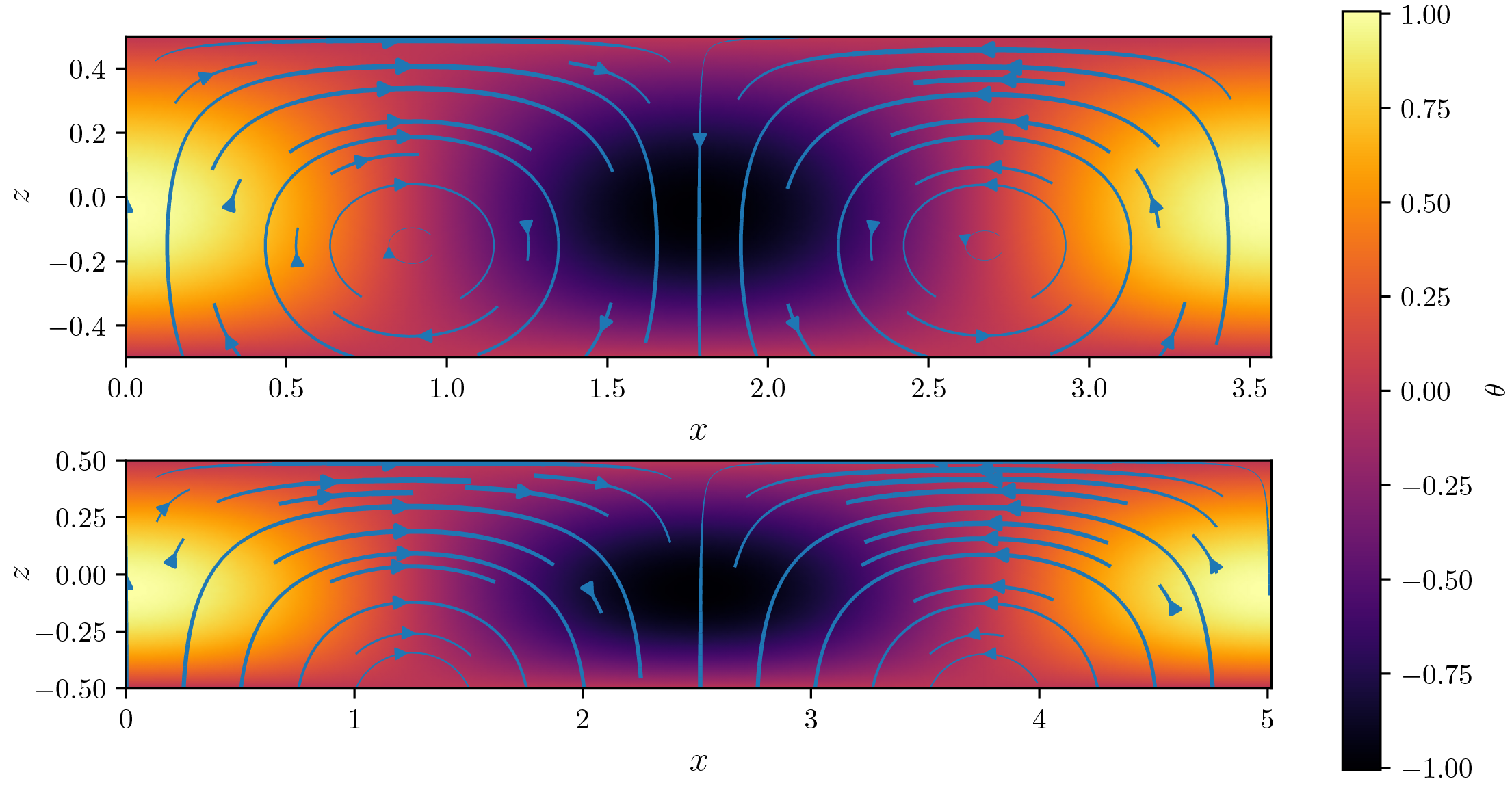
Figure 12: First unstable mode when only the bottom boundary is a phase change interface, with $\Phi^{-}=10$ (top) and $\Phi^{-}=10^{-2}$ (bottom). The temperature anomaly compared to the conduction solution is represented in colours and streamlines have a thickness proportional to the relative norm of the velocity.

Figure 13 shows the variation of the critical Rayleigh number (top) and wavenumber (bottom) as a function of $\Phi^{-}$ and one can see that both tend to a finite value when $\Phi^{-}\rightarrow 0$. The mode obtained for $\Phi^{-}=10^{-2}$ is close to that limit. Contrary to the situation with a phase change at both boundaries, the presence of non-penetrating boundary condition implies that some deformation is always needed for convection to occurs, which makes viscosity still be a limiting factor at vanishing values of $\Phi^{-}$.

Figure 13: Critical Rayleigh number (top) and wavenumber (bottom) as function of the phase change number for the bottom boundary $\Phi^{-}$, the top one having a non-penetrating condition. The dash dotted lines represent the classical values obtained for two non-penetrating conditions, for reference.

Figure 14: Heat flux coefficient as a function of the bottom phase change number $\Phi^{-}$, the top boundary being non-penetrative (left), and Nusselt number as a function of Rayleigh number for different values of $\Phi^{-}$ (right).

Considering now the weakly non-linear analysis results, figure 14 shows that the heat flux coefficient for only one phase change boundary condition tends to a little above 1, that is about half that for the case for both non-penetrative boundaries. Combining that with a critical Rayleigh number that is about four times smaller makes $\operatorname{d\!}{\mbox{{Nu}}}/\operatorname{d\!}{\mbox{{Ra}}}$ about twice that for the classical situation. Therefore, the efficiency of heat transfer is improved compared to the classical case, both because convection starts for a smaller Rayleigh number and because the rate of variation of the Nusselt number with Ra is about twice larger. This is illustrated on the right panel of figure 14.

Figure 15: Mean temperature coefficient ($B$ defined in equation (93)) as function of the bottom phase change parameter $\Phi^{-}$ (left) and mean temperature as function of Ra for different values of $\Phi^{-}$ (right). The range of Ra values explored is the same as that used for figure 14.

In contrary to the case with both boundaries being a phase change with equal values of $\Phi$, the case discussed in this section breaks the symmetry around the $z=0$ plane. In particular, this means that the mean temperature in the domain is not equal to the average of both boundaries, $\langle T\rangle\neq 1/2$ in dimensionless form. As for the Nusselt number (eq. 86), a contribution from all even orders in $\epsilon$ is expected, and to the leading order explored here,

$$\langle T\rangle=\frac{1}{2}+\langle\theta_{2,0}\rangle\frac{\mbox{{Ra}}_{c}}{\mbox{{Ra}}_{2}}\frac{\mbox{{Ra}}-\mbox{{Ra}}_{c}}{\mbox{{Ra}}_{c}}\equiv\frac{1}{2}+B\frac{\mbox{{Ra}}-\mbox{{Ra}}_{c}}{\mbox{{Ra}}_{c}}.$$ (93)

The coefficient $B$ defined above is computed exactly for the case of both non-penetrating boundaries and as expected found to be null. Figure 15 shows the evolution of this coefficient as function of $\Phi^{-}$. One can see that it tends to a finite positive value when in the limit $\Phi^{-}\rightarrow 0$. Therefore, for small values of $\Phi^{-}$, the average temperature is expected to be larger than $1/2$ (figure 15). For the same range of Rayleigh number as explored in figure 14, figure 15 also shows the evolution of the mean temperature at the leading order given by equation (93). For low values of $\Phi^{-}$, the mean temperature increases rapidly with Rayleigh number.

Figure 16: Finite amplitude solution for $\Phi^{-}=10^{-2}$, $\epsilon=5.58$ and a non-penetrating boundary condition at the top.

The asymmetry of the mean temperature for low values of $\Phi^{-}$ is also expressed in the finite amplitude solution that can be plotted for a given value of $\epsilon$. The range of validity of such solutions as function of $\epsilon$ depends on the order of the development. Computing the solution only up to order 3 in $\epsilon$, we restrict ourselves to small values of this number and figure 16 shows the result for $\epsilon=5.58$ corresponding to $\mbox{{Nu}}=1.5$. This shows that the down-welling current is more focused than the up-welling one. This situation is similar to the case of volumetrically heated convection (e. g. Parmentier & Sotin, 2000), which is not the case here. Preliminary direct numerical simulations confirm this behaviour but the full exploration of this question goes beyond the scope of the present paper.

6 Conclusion

In the context of the dynamics of planetary mantles, convection can happen in solid shells adjacent to liquid layers. The viscous stress in the solid builds up a topography of the interface between the solid and liquid layers. In the absence of mechanisms to erase topography, its buoyancy equilibrates the viscous stress which effectively enforces a non-penetrating boundary condition. On the other hand, if the topography can be suppressed by melting and freezing at the interface at a faster pace than its building process, the vertical velocity is not required to be null at the interface. The non-penetrating boundary condition is then replaced by a relationship between the normal velocity, its normal gradient, and pressure (eq. 16) and involving a dimensionless phase change number, $\Phi$, ratio of the phase change timescale to the viscous timescale (eq. 15). When this number is large, we recover the classical non-penetrating condition while the limit of low $\Phi$ authorises a large flow through the boundary.

When both boundaries are characterised by a low $\Phi$ number, a translating, non-deforming, mode of convection is possible and competes with a deforming mode with wave number $k$ that decreases as $\sqrt{\Phi}$, and therefore ressembles translation with alternating up- and downward direction. The critical Rayleigh number for the onset of the deforming mode is slightly below that of the translation mode, $\mbox{{Ra}}=24\Phi$, but the latter is found to be stable against a deforming instability when the Rayleigh number is $\sim\Phi^{2}$ above the critical value. It is therefore likely to dominate when both boundaries are characterised by low values of $\Phi$. In both translating and deforming modes of convection, the heat transfer efficiency, the Nusselt number, is found to increase strongly with Rayleigh number at small values of $\Phi$.

When only one boundary is a phase change interface with a low value of $\Phi$, the wavenumber is about half and the critical Rayleigh number is about a quarter the corresponding values for the classical non-penetrating boundary condition. Close to onset, a weakly non-linear analysis shows that the Nusselt number varies linearly with the Rayleigh number with a slope that is about twice that for both non-penetrating boundary conditions. The average temperature is also found to increase strongly with Rayleigh number and the flow geometry is strongly affected, with down-welling currents more focused than up-welling ones.

Overall, having the possibility of melting and freezing across one or both horizontal boundaries of an infinite Prandtl number fluid makes convection much easier (i.e. the critical Rayleigh number is strongly reduced), the preferred horizontal wavelength much larger and heat transfer much stronger, with important potential implications for planetary dynamics.

7 Acknowledgments

We are thankful to three anonymous reviewers and editor Grae Worster for comments that pushed us to significantly clarify our paper. This research has been funded by the french Agence Nationale de la Recherche under the grant number ANR-15-CE31-0018-01, MaCoMaOc.

Appendix A Self-adjointness of operator $\mathbf{L}_{c}$

Using a Fourier decomposition for the horizontal decomposition, $\mathbf{L}_{c}$ simply reads as

$$\mathbf{L}_{c}=\left(\begin{array}[]{cccc}0&\mathrm{i}k&\operatorname{D\!}&0\\ -\mathrm{i}k&\operatorname{D\!}^{2}-k^{2}&0&0\\ -\operatorname{D\!}&0&\operatorname{D\!}^{2}-k^{2}&\mbox{{Ra}}_{c}\\ 0&0&1&\operatorname{D\!}^{2}-k^{2}\end{array}\right)$$ (94)

where the time derivative has been omitted since the linear instability is found to be stationary. In a linear stability analysis, adding a growth rate $\sigma$ on the diagonal of the matrix would not alter the adjoint calculation, as will appear below. The boundary conditions are given by equations (52) to (54). In the calculation of the dot product, the $\theta$ part is given $\mbox{{Ra}}_{c}$ as weight and the horizontal integral can be factored out:

$$\begin{split}\braket{\mathbf{X}_{2}}{\mathbf{L}_{c}\mathbf{X}_{1}}=&\int\mathrm{e}^{\mathrm{i}(k_{2}-k_{1})}\operatorname{d\!}{x}\left[\int_{-\frac{1}{2}}^{\frac{1}{2}}\bar{P}_{2}\left(\mathrm{i}kU_{1}+\operatorname{D\!}W_{1}\right)\operatorname{d\!}{z}\right.\\ &+\int_{-\frac{1}{2}}^{\frac{1}{2}}\bar{U}_{2}\left(-\mathrm{i}kP_{1}+\left(\operatorname{D\!}^{2}-k^{2}\right)U_{1}\right)\operatorname{d\!}{z}\\ &+\int_{-\frac{1}{2}}^{\frac{1}{2}}\bar{W}_{2}\left(-\operatorname{D\!}P_{1}+\left(\operatorname{D\!}^{2}-k^{2}\right)W_{1}+\mbox{{Ra}}_{c}\Theta_{1}\right)\operatorname{d\!}{z}\\ &\left.+\mbox{{Ra}}_{c}\int_{-\frac{1}{2}}^{\frac{1}{2}}\bar{\Theta}_{2}\left(W_{1}+\left(\operatorname{D\!}^{2}-k^{2}\right)\Theta_{1}\right)\operatorname{d\!}{z}\right]\end{split}$$ (95)

where the overbar means complex conjugate. Since the $x$ part poses no difficulty, we only consider the $z$ part, which we denote as $\braket{\bullet}{\bullet}_{z}$. Reordering the different integrals in Eq. (95) so that terms of $\mathbf{X}_{1}$ are factored out and performing integrations by part on each term including $\operatorname{D\!}$, we get

$$\begin{split}\braket{\mathbf{X}_{2}}{\mathbf{L}_{c}\mathbf{X}_{1}}_{z}=&\int_{-\frac{1}{2}}^{\frac{1}{2}}\left(-\mathrm{i}k\bar{U}_{2}+\operatorname{D\!}\bar{W}_{2}\right)P_{1}\operatorname{d\!}{z}\\ &+\int_{-\frac{1}{2}}^{\frac{1}{2}}\left(\mathrm{i}k\bar{P}_{2}+\left(\operatorname{D\!}^{2}-k^{2}\right)\bar{U}_{2}\right)U_{1}\operatorname{d\!}{z}\\ &+\int_{-\frac{1}{2}}^{\frac{1}{2}}\left(\operatorname{D\!}\bar{P}_{2}+\left(\operatorname{D\!}^{2}-k^{2}\right)\bar{W}_{1}+\mbox{{Ra}}_{c}\bar{\Theta}_{2}\right)W_{1}\operatorname{d\!}{z}\\ &+\mbox{{Ra}}_{c}\int_{-\frac{1}{2}}^{\frac{1}{2}}\left(\bar{W}_{2}+\left(\operatorname{D\!}^{2}-k^{2}\right)\bar{\Theta}_{2}\right)\Theta_{1}\operatorname{d\!}{z}\\ &+\left[\bar{P}_{2}W_{1}\right]_{-\frac{1}{2}}^{\frac{1}{2}}+\left[\bar{U}_{2}\operatorname{D\!}{U}_{1}\right]_{-\frac{1}{2}}^{\frac{1}{2}}-\left[U_{1}\operatorname{D\!}{\bar{U}_{2}}\right]_{-\frac{1}{2}}^{\frac{1}{2}}-\left[\bar{W}_{2}P_{1}\right]_{-\frac{1}{2}}^{\frac{1}{2}}\\ &+\left[\bar{W}_{2}\operatorname{D\!}{W}_{1}\right]_{-\frac{1}{2}}^{\frac{1}{2}}-\left[W_{1}\operatorname{D\!}{\bar{W}_{2}}\right]_{-\frac{1}{2}}^{\frac{1}{2}}+\mbox{{Ra}}\left(\left[\bar{\Theta}_{2}\operatorname{D\!}{\Theta}_{1}\right]_{-\frac{1}{2}}^{\frac{1}{2}}-\left[\Theta_{1}\operatorname{D\!}{\bar{\Theta}_{2}}\right]_{-\frac{1}{2}}^{\frac{1}{2}}\right)\end{split}$$ (96)

The integral part shows that the adjoint linear system is the same as the direct one, with $\mathbf{L}_{c}$ as operator. The boundary conditions are the one that allow to suppress all the boundary values in equation (96). The boundary conditions (52) to (54) are applied to $\mathbf{X}_{1}$ to remove $\Theta_{1}(\pm\frac{1}{2})$ and replace $\operatorname{D\!}{U}_{1}$ and $P_{1}$. In addition, the mass conservation equation applied to $\mathbf{X}_{2}$ allows to replace $\operatorname{D\!}{W}_{2}$. Factorizing $W_{1}$, $U_{1}$ and $\Theta_{1}$ gives for the boundary conditions

$$\left[W_{1}\left(-\bar{P}_{2}\pm\Phi^{\pm}\bar{W}_{2}+2\operatorname{D\!}{\bar{W}_{2}}\right)\right]_{-\frac{1}{2}}^{\frac{1}{2}}+\left[U_{1}\left(-\mathrm{i}k\bar{W}_{2}+\operatorname{D\!}{\bar{U}_{2}}\right)\right]_{-\frac{1}{2}}^{\frac{1}{2}}-\mbox{{Ra}}\left[\bar{\Theta}_{2}\operatorname{D\!}{\Theta}_{1}\right]_{-\frac{1}{2}}^{\frac{1}{2}}=0.$$ (97)

Since $W_{1}$, $U_{1}$ and $\operatorname{D\!}{\Theta}_{1}$ can take arbitrary values on the boundaries, the differences can only be eliminated in a general manner by setting all their coefficients to 0, which gives the boundary conditions for the adjoint:

$$\operatorname{D\!}U_{2}+\mathrm{i}kW_{2} =0,$$ (98)

$$\pm\Phi^{\pm}W_{2}+2\operatorname{D\!}W_{2}-P_{2} =0,$$ (99)

$$\Theta_{2} =0.$$ (100)

The adjoint problem is therefore identical to the direct one. Among other implications, all eigenvalues of $L_{c}$ must be real, which is consistent with our numerical findings.

Appendix B Expression of the non-linear terms

Computation of the non-linear term $\mathbf{N}(\mathbf{X}_{n},\mathbf{X}_{m})$ (eq. 70) is the trickiest part of the procedure explained in section 4.2 and deserves some details provided here. First of all, it contains only a $\mathbf{\Theta}$ component, referred to as $\mathbf{N}(\mathbf{X}_{n},\mathbf{X}_{m})_{\Theta}$. To compute it, one needs first to decompose indices $n$ and $m$ as

$$n =2p+q\mbox{ with }p=\left\lfloor\frac{n}{2}\right\rfloor,$$ (101)

$$m =2r+s\mbox{ with }r=\left\lfloor\frac{m}{2}\right\rfloor,$$ (102)

where $\lfloor\rfloor$ denotes the floor function. In computing $\mathbf{N}(\mathbf{X}_{n},\mathbf{X}_{m})_{\Theta}$, one needs to account for the full (i.e. real) expression of $\mathbf{X}_{n}$ and $\mathbf{X}_{m}$ including the complex conjugate. They write

$$\mathbf{X}_{n} =\sum_{l_{1}=0}^{p}\mathbf{Z}_{n,2l_{1}+q}(z)\mathrm{e}^{\mathrm{i}(2l_{1}+q)kx}+c.c.,$$ (103)

$$\mathbf{X}_{m} =\sum_{l_{2}=0}^{r}\mathbf{Z}_{m,2l_{1}+s}(z)\mathrm{e}^{\mathrm{i}(2l_{2}+s)kx}+c.c..$$ (104)

Using eq. (70), we get

$$\begin{split}\mathbf{N}(\mathbf{X}_{n},\mathbf{X}_{m})_{\Theta}=\sum_{l_{1}=0}^{p}\sum_{l_{2}=0}^{q}&\left\{\left[\mathrm{i}(2l_{2}+s)kU_{n,2l_{1}+q}\Theta_{m,2l_{2}+s}\right.\right.\\ &\left.+W_{n,2l_{1}+q}D\Theta_{m,2l_{2}+s}\right]\mathrm{e}^{\mathrm{i}[2(l_{1}+l_{2})+q+s]kx}\\ &+\left[-\mathrm{i}(2l_{2}+s)kU_{n,2l_{1}+q}\bar{\Theta}_{m,2l_{2}+s}\right.\\ &\left.\left.+W_{n,2l_{1}+q}D\bar{\Theta}_{m,2l_{2}+s}\right]\mathrm{e}^{\mathrm{i}(2(l_{1}-l_{2})+q-s)kx}\right\}+c.c..\end{split}$$ (105)

The harmonics of the first term is always positive while that of the second can be negative. Either way, each term has its complex conjugate and we solve only for the positive or null harmonics, the rest of the solution simply being obtained as the conjugate of the computed part.

References

- Alboussière et al. (2010) Alboussière, T., Deguen, R. & Melzani, M. 2010 Melting-induced stratification above the Earth’s inner core due to convective translation. Nature 466, 744–747.
- Baland et al. (2014) Baland, R.-M., Tobie, G., Lefèvre, A. & Hoolst, T. Van 2014 Titan’s internal structure inferred from its gravity field, shape, and rotation state. Icarus 237 (0), 29 – 41.
- Bercovici & Ricard (2014) Bercovici, David & Ricard, Yanick R 2014 Plate tectonics, damage and inheritance. Nature 508, 513–516.
- Čadek et al. (2016) Čadek, O, Tobie, G, Van Hoolst, T, Massé, M, Choblet, G, Lefèvre, A, Mitri, G, Baland, R-M, Běhounková, M, Bourgeois, O & Trinh, A 2016 Enceladus’s internal ocean and ice shell constrained from Cassini gravity, shape, and libration data. Geophys. Res. Lett. 43 (11), 5653–5660, 2016GL068634.
- Canuto et al. (1988) Canuto, C., Hussaini, M., Quarteroni, A. & Zang, T. 1988 Spectral methods in fluid dynamics. New York: Springer-Verlag.
- Christensen & Yuen (1989) Christensen, Ulrich R. & Yuen, David A. 1989 Time-dependent convection with non-newtonian viscosity. J. Geophys. Res. 94 (B1), 814–820.
- Crank (1984) Crank, John 1984 Free and moving boundary problems. Oxford: Oxford University Press, 425 pp.
- Cross & Hohenberg (1993) Cross, M. C. & Hohenberg, P. C. 1993 Pattern formation outside of equilibrium. Rev. Modern Phys. 65 (3), 851–1112.
- Davaille & Jaupart (1993) Davaille, A. & Jaupart, C. 1993 Transient high-Rayleigh-number thermal convection with large viscosity variations. J. Fluid Mech. 253, 141–166.
- Deguen (2013) Deguen, R. 2013 Thermal convection in a spherical shell with melting/freezing at either or both of its boundaries. J. Earth Sci. 24, 669–682.
- Deguen et al. (2013) Deguen, R., Alboussière, T. & Cardin, P. 2013 Thermal convection in Earth’s inner core with phase change at its boundary. Geophys. J. Int. 194, 1310–1334.
- Elkins-Tanton (2012) Elkins-Tanton, L. T 2012 Magma oceans in the inner solar system. Ann. Rev. Earth Planet. Sci. 40, 113–139.
- Gaidos & Nimmo (2000) Gaidos, E. J. & Nimmo, F. 2000 Planetary science: Tectonics and water on Europa. Nature 405 (6787), 637–+.
- Grasset et al. (2000) Grasset, O., Sotin, C. & Deschamps, F. 2000 On the internal structure and dynamics of titan. Planet. Space Sci. 48 (7–8), 617–636.
- Guo et al. (2012) Guo, W., Labrosse, G. & Narayanan, R. 2012 The Application of the Chebyshev-Spectral Method in Transport Phenomena. Berlin: Springer-Verlag.
- Jarvis & McKenzie (1980) Jarvis, G. T. & McKenzie, D. P. 1980 Convection in a compressible fluid with infinite Prandtl number. J. Fluid Mech. 96, 515–583.
- Jeffreys (1930) Jeffreys, H. 1930 The instability of a compressible fluid heated below. Math. Proc. Camb. Phil. Soc. 26, 170–172.
- Khurana et al. (1998) Khurana, K. K., Kivelson, M. G., Stevenson, D. J., Schubert, G., Russell, C. T., Walker, R. J. & Polanskey, C. 1998 Induced magnetic fields as evidence for subsurface oceans in europa and callisto. Nature 395 (6704), 777–780.
- Labrosse et al. (2007) Labrosse, S., Hernlund, J. W. & Coltice, N. 2007 A crystallizing dense magma ocean at the base of Earth’s mantle. Nature 450, 866–869.
- Malkus & Veronis (1958) Malkus, W.V.R. & Veronis, G. 1958 Finite amplitude cellular convection. J. Fluid Mech. 4, 225–260.
- Manneville (2004) Manneville, P. 2004 Instabilities, Chaos and Turbulence - An introduction to nonlinear dynamics and complex systems. London: Imperial College Press.
- McKenzie et al. (1974) McKenzie, D. P., Roberts, J. M. & Weiss, N. O. 1974 Convection in the Earth’s mantle: towards a numerical simulation. J. Fluid Mech. 62, 465–538.
- Mizzon & Monnereau (2013) Mizzon, H. & Monnereau, M. 2013 Implication of the lopsided growth for the viscosity of Earth’s inner core. Earth Planet. Sci. Lett. 361, 391 – 401.
- Monnereau et al. (2010) Monnereau, M, Calvet, M, Margerin, L & Souriau, A 2010 Lopsided growth of Earth’s inner core. Science 328 (5981), 1014–1017.
- Monnereau & Dubuffet (2002) Monnereau, M. & Dubuffet, F. 2002 Is io’s mantle really molten? Icarus 158, 450–59.
- Pappalardo et al. (1998) Pappalardo, R. T., Head, J. W., Greeley, R., Sullivan, R. J., Pilcher, C., Schubert, G., Moore, W. B., Carr, M. H., Moore, J. M., Belton, M. J. S. & Goldsby, D. L. 1998 Geological evidence for solid-state convection in Europa’s ice shell. Nature 391 (6665), 365–368.
- Parmentier (1978) Parmentier, E. M. 1978 Study of thermal-convection in non-newtonian fluids. J. Fluid Mech. 84, 1–11.
- Parmentier & Sotin (2000) Parmentier, E. M. & Sotin, C 2000 Three-dimensional numerical experiments on thermal convection in a very viscous fluid: Implications for the dynamics of a thermal boundary layer at high Rayleigh number. Phys. Fluids 12 (3), 609–617.
- Pedlosky (1987) Pedlosky, J. 1987 Geophysical Fluid Dynamics, 2nd edn. New York: Springer-Verlag.
- Rayleigh (1916) Rayleigh, Lord 1916 On convection currents in a horizontal layer of fluid, when the higher temperature is on the under side. Phil. Mag. 32, 529–546.
- Ricard et al. (2014) Ricard, Y., Labrosse, S. & Dubuffet, F. 2014 Lifting the cover of the cauldron: Convection in hot planets. Geochem. Geophys. Geosyst. 15, 4617–4630.
- Roberts & King (2013) Roberts, P H & King, E M 2013 On the genesis of the Earth’s magnetism. Rep. Prog. Phys. 76 (9), 6801.
- Schlüter et al. (1965) Schlüter, A., Lortz, D. & Busse, F. 1965 On the stability of steady finite amplitude convection. J. Fluid Mech. 23, 129–144.
- Schubert et al. (2001) Schubert, G., Turcotte, D. L. & Olson, P. 2001 Mantle Convection in the Earth and Planets. Cambridge: Cambridge University Press.
- Soderlund et al. (2014) Soderlund, K. M., Schmidt, B. E., Wicht, J. & Blankenship, D. D. 2014 Ocean-driven heating of europa/’s icy shell at low latitudes. Nature Geosci 7 (1), 16–19.
- Sohl et al. (2003) Sohl, F., Hussmann, H., Schwentker, B., Spohn, T. & Lorenz, R. D. 2003 Interior structure models and tidal love numbers of titan. J. Geophys. Res. 108 (E12).
- Solomatov (2007) Solomatov, V. S. 2007 Magma oceans and primordial mantle differentiation. Treatise on Geophysics 9, 91–120.
- Tackley (2000) Tackley, Paul J. 2000 Self-consistent generation of tectonic plates in time-dependent, three-dimensional mantle convection simulations 1. pseudoplastic yielding. Geochem. Geophys. Geosys. 1, 2000Gc000041.
- Tobie et al. (2003) Tobie, G., Choblet, G. & Sotin, C. 2003 Tidally heated convection: Constraints on Europa’s ice shell thickness. J. Geophys. Res. 108, 5124.
- Turcotte & Oxburgh (1967) Turcotte, D. L. & Oxburgh, E. R. 1967 Finite amplitude convective cells and continental drift. J. Fluid Mech. 28, 29–42.
- Turcotte & Schubert (2001) Turcotte, D. L. & Schubert, G. 2001 Geodynamics, 2nd edn. Cambridge, UK: Cambridge University Press.
- Weideman & Reddy (2000) Weideman, J. A. & Reddy, S. C. 2000 A matlab differentiation matrix suite. ACM Trans. Math. Softw. 26 (4), 465–519.