Approximate Solution of Length-Bounded Maximum Multicommodity Flow with Unit Edge-Lengths

Abstract

An improved fully polynomial-time approximation scheme and a greedy heuristic for the fractional length-bounded maximum multicommodity flow problem with unit edge-lengths are proposed. Computational experiments are carried out on benchmark graphs and on graphs that model software defined satellite networks to compare the proposed algorithms and an exact linear programming solver. The results of experiments demonstrate a trade-off between the computing time and the precision of algorithms under consideration.

Keywords: Fully Polynomial-Time Approximation Scheme, Quality of Service, Software Defined Satellite Network

1 Introduction

Research issues in telecommunications often involve requirements to quality of service such as bandwidth, delay, number of hops, etc. [14, 18]. These research issues may be interpreted as combinatorial optimization problems of finding a multicommodity flow through the network that satisfies some quality of service constraints.

Multicommodity flow (MCF) problems are defined on a directed graph $G=(V,E)$ with edge capacities $u:E\to\mathbb{R}$ and $k$ origin-to-destination pairs $(s_{j},t_{j}),$ $j=1,\dots,k$. These problems ask for a family of flows $f_{j}$ from $s_{j}$ to $t_{j}$, so that some optimization criterion is maximized under the node flow conservation constraints and the requirement that the sum of flows on any edge does not exceed the capacity of the edge.

In particular, the maximum multicommodity flow problem (maximum MCF for short) is an MCF problem where the total flow needs to be maximized. Some authors assume that the maximum MCF also includes an assumption that the value of each flow $f_{j}$ is limited by a finite demand $d_{j},\ j=1,\dots,k$ (see e.g. [18]).

A more general problem, called fractional length-bounded maximum multicommodity flow (fractional length-bounded maximum MCF for short), asks for computing the maximum MCF routed along a set of paths whose length does not exceed a specific bound. This problem was studied in [2, 3] assuming unbounded demands and in [5], assuming that finite demands are given. In particular, it was shown in [2] that the fractional length-bounded maximum MCF is NP-complete, while its special case where all edges have unit length is polynomially solvable.

A modification of the fractional length-bounded maximum MCF with an additional constraint that the flow on all edges must be integer-valued is called integral length-bounded maximum MCF. The results from [9] show that even when there is no length constraint at all, the edge capacities are equal to 1, and the graph is outerplanar, this problem does not admit approximation algorithms with constant approximation ratios, unless P=NP. A result from [10] implies that the integral length-bounded maximum MCF can not be approximated with a performance ratio $1/n^{0.5-\varepsilon}$ for any $\varepsilon>0$ in the special case where all edges have equal length and all edge capacities are equal to 1, assuming P$\neq$NP. Complexity and non-approximability of this problem was also studied in [2, 4].

Fully polynomial time approximation schemes (FPTAS) for fractional length-bounded maximum MCF were proposed in [2, 5]. In [18], an FPTAS was shown to exist for a more general quality of service-aware MCF problem (QoS-aware max-flow). The present paper is aimed at fast approximate solution of a special case of fractional length-bounded maximum MCF where all edges have the length equal to one.

In Section 2, we give a formal statement of fractional length-bounded maximum MCF and describe some basic properties of this problem. In Section 3, using the approach from [7] and the improvement of [6] we develop an FPTAS for a special case of the problem where all edges have unit length. This FPTAS has a smaller time complexity compared to the FPTAS from [18] which was developed for arbitrary edge lengths. In Section 4, we propose a simple greedy heuristic applicable to fractional length-bounded maximum MCF as well as integral length-bounded maximum MCF (assuming unit edge lengths in both cases). In Section 5, we compare these algorithms to each other and to IBM CPLEX solver in computational experiments. The last section contains conclusions.

2 Problem Formulations and Basic Properties

A flow in a digraph $G=(V,E)$ from origin vertex $s\in V$ to destination vertex $t\in V$ is a nonnegative function $f:E\to R_{+}$ such that for each node $v\in V,\ v\neq s,\ v\neq t$ holds

$$\sum_{(v^{\prime},v)\in E}f(v^{\prime},v)-\sum_{(v,v^{\prime})\in E}f(v,v^{\prime})=0$$

and

$$|f|=\sum_{(s,v^{\prime})\in E}f(s,v^{\prime})-\sum_{(v^{\prime},s)\in E}f(v^{\prime},s)=\sum_{(v^{\prime},t)\in E}f(v^{\prime},t)-\sum_{(t,v^{\prime})\in E}f(t,v^{\prime})$$

is the amount of flow sent from $s$ to $t$ in $f$. If $P_{1},\dots,P_{r}$ are paths from $s$ to $t$, then a sum of path-flows along $P_{1},\dots,P_{r}$ gives a network flow from $s$ to $t$ again. Given that $f=\sum_{j=1}^{r}f^{P_{j}}$, we will say that $f$ is routed along the set of paths $P_{1},\dots,P_{r}$.

We will assume that flow $f_{i}$ of commodity $i,i=1,\dots,k,$ has an origin $s_{i}\in V$ and a destination $t_{i}\in V$. If $f_{1},f_{2},\dots,f_{k}$ are flows of $k$ commodities, then $F=(f_{1},f_{2},\dots,f_{k})$ is called a multicommodity flow in $G$.

An input instance of the maximum MCF consists of a directed network ${G=(V,E)}$, where $|V|=n,\ |E|=m$, an edge capacity function ${u:E\to\mathbb{R}_{+}}$ and a specification $(s_{i},t_{i},d_{i})\in V\times V\times\mathbb{R}^{+}$ of commodity $i$ for $i=1,\dots,k$. The objective is to maximize $\sum_{i=1}^{k}|f_{i}|,$ so that the sum of flows on any edge $e\in E$ does not exceed $u(e)$ and $|f_{i}|\leq d_{i},\ i=1,\dots,k$.

The fractional length-bounded maximum MCF has the same input, extended by an upper bound $L\in\mathbb{Z}^{+}$ and the edge lengths $\tau(e),\ e\in E$ and asks for a maximum MCF where the sum of flows on any $e\in E$ does not exceed $u(e)$, $|f_{i}|\leq d_{i},\ i=1,\dots,k,$ and the flow of each commodity is routed along a set of paths, where each path has a length at most $L$. A special case of this problem where all edges have a unit length requires that the flow of each commodity is routed along a set of paths at most $L$ edges long. In what follows, we will denote fractional length-bounded maximum MCF problem by LBMCF and its special case where all edges have unit length will be denoted by LBMCF1. Obviously, the maximum MCF may be considered a special case of LBMCF1, assuming $L=n$. W.l.o.g. we will assume that all pairs $(s_{i},t_{i})$ are unique, since otherwise the demands with identical pairs $(s_{i},t_{i})$ may be summed together in one demand.

LBMCF1 is polynomially equivalent to its special case with unbounded demands. Indeed, given an LBMCF1 instance ${G=(V,E)}$, ${u:E\to\mathbb{R}_{+}}$, $(s_{i},t_{i},d_{i}),$ $i=1,\dots,k$ and $L$, consider a new instance of this problem with unbounded demands on a network $G^{\prime}$, obtained from $G$ as described below. Let $T_{v}\subset V$ be the set of all vertices where at least one commodity originating in $v$ is consumed, i.e. $T_{v}:=\cup_{i:s_{i}=v}\{t_{i}\}$. For each vertex $v\in V$ with $|T_{v}|>0$:

• New $|T_{v}|$ vertices are created and connected by arcs leading into vertex $v$.

• The new vertices are assigned to commodities with destinations in $T_{v}$ by a one-to-one mapping. So we can denote the new vertices connected to $v$ as $v_{i}$ where $i$ is such that $s_{i}=v$.

• The capacities of edges leading from vertices $v_{i}$ to $v$ are set to $d_{i}$.

In the new problem the demands are $(v_{i},t_{i},+\infty),$ $i=1,\dots,k$ and the new upper bound is $L^{\prime}=L+1.$

There is a bijection between the sets of feasible solutions of the original instance and the new instance and the objective function values of the corresponding solutions are equal. Now since the special case of LBMCF1 with unbounded demands is solvable by LP methods in weakly polynomial time [2], the above reduction implies that LBMCF1 with finite demands is also solvable in weakly polynomial time (the same follows from the LP formulation of this problem (1)–(4) presented below). The question of solvability of LBMCF1 in strongly polynomial time remains open. In the special case of maximum MCF, a strongly polynomial algorithm is known [17]. Nevertheless, even in this special case existence of exact algorithms using the same combinatorial techniques as the Ford-Fulkerson method for the single-commodity flow is unlikely (see e.g. [15], § 70.13).

In the special case of maximum MCF there is a well-known formulation the problem in terms of the LP using edge flows (see e.g. [11], § 11) with $O(k+m)$ constraints and $O(km)$ variables. Assuming that variables ${x_{i}(e)\geq 0}$ give the amount of flow of commodity $i$ over edge $e$ the LP model is as follows.

$$\max\sum_{i=1}^{k}\ \sum_{e=(s_{i},v)\in E}\ x_{i}(e),$$ (1)

$$\sum_{e=(s_{i},v)\in E}x_{i}(e)\leq d_{i},\ \ i=1,\dots,k,$$ (2)

$$\sum_{i=1}^{k}x_{i}(e)\leq u(e),\ \ e\in E,$$ (3)

$$\sum_{e=(v^{\prime},v)\in E}x_{i}(e)=\sum_{e=(v,v^{\prime})\in E}x_{i}(e),\ \ i=1,\dots,k,\ \ v\in V\backslash\{s_{i},t_{i}\},$$ (4)

An LP formulation of LBMCF1, involving ${O(Lkn+m)}$ constraints and $O(Lkm)$ variables, may be constructed using a multicommodity flow in a supplementary time-expanded network [12]. The node set $V^{\prime}$ contains a copy $V_{t}$ of the node set $V$ of graph $G$ for every discrete time step $t,t=1,\dots,L$. For every directed edge $(v,w)\in E$ there is an edge in $E^{\prime}$ from vertex $v_{t}\in V_{t}$ in time layer $t$ to vertex $w_{t+1}\in V_{t+1}$. Besides that, $E^{\prime}$ contains edges $(v_{t},v_{t+1})$ for all $v_{t}\in V_{t},\ t=1,\dots,L-1.$ A multicommodity flow is sought in this time-expanded network under additional constraints which require that for each $e=(v,w)\in E$ the sum of all flows traversing the edges $(v_{t},w_{t+1}),\ t=1,\dots,L-1$ is at most $u(e).$ For all $i=1,\dots,k,$ the origin of commodity $i$ is placed in the copy $s_{i1}$ of vertex $s_{i}$ at level 1 and the destination is placed in the copy $t_{iL}$ of vertex $t_{i}$ at level $L$. The resulting LP formulation is as follows

$$\max\sum_{i=1}^{k}\ \sum_{e^{\prime}=(s_{i1},v_{2})\in E^{\prime}}\ x_{i}(e^{\prime}),$$ (5)

$$\sum_{e^{\prime}=(s_{i1},v_{2})\in E^{\prime}}x_{i}(e^{\prime})\leq d_{i},\ \ i=1,\dots,k,$$ (6)

$$\sum_{i=1}^{k}\sum_{e^{\prime}=(v_{t},w_{t+1})\in E^{\prime}}x_{i}(e^{\prime})\leq u(e),\ \ e=(v,w)\in E,$$ (7)

$$\sum_{e^{\prime}=(v_{t-1},w_{t})\in E^{\prime}}x_{i}(e^{\prime})=\sum_{e^{\prime}=(w_{t},v_{t+1})\in E^{\prime}}x_{i}(e^{\prime}),$$ (8)

$$i=1,\dots,k,\ \ w_{t}\in V_{t},\ \ t=2,\dots,L-1,$$

$$\sum_{e^{\prime}=(v_{L-1},w_{L})\in E^{\prime}}x_{i}(e^{\prime})=0,\ \ i=1,\dots,k,\ \ w_{L}\in V_{L}\backslash\{t_{Li}\},$$ (9)

where variables $x_{i}(e^{\prime})\geq 0$ give the amount of flow of commodity $i$ over edge $e^{\prime}\in E^{\prime}$.

The practice shows that large MCF problems require a long time and a great amount of memory to solve using the exact LP methods either in path flow-based or edge flow-based formulations. (see e.g. [15], § 70.13). For this reason, it is important to develop faster algorithms to solve MCF problems approximately and LBMCF1 among them.

A feasible solution $y$ to a maximization problem is called a $(1-\omega)$-approximate if it satisfies the inequality $f(y)\geq(1-\omega)f^{*},$ where $\omega>0$ and $f^{*}$ is the optimal objective function value. An algorithm is called a $(1-\omega)$-approximation algorithm if in a polynomially bounded time it outputs a $(1-\omega)$-approximate solution given a solvable problem instance. A family of $(1-\omega)$-approximation algorithms parameterized by $\omega>0$, such that the time complexity of these algorithms is polynomially bounded in $1/\omega$ and in the problem instance length is called a fully polynomial-time approximation scheme (FPTAS).

3 Fully Polynomial Time Approximation Scheme

3.1 The Case of Unbounded Demands

This subsection presents an FPTAS for LBMCF1 with unbounded demands, which is developed analogously to the FPTAS for maximum MCF with unbounded demands [6].

Let ${\mathcal{P}}_{i}$ denote the set of all paths from $s_{i}$ to $t_{i}$ in $G$ and let ${\mathcal{P}}_{i}(L)$ denote the subset of ${\mathcal{P}}_{i}$ which consists of paths at most $L$ edges long. Besides that, put ${\mathcal{P}}(L)=\cup_{i=1}^{k}{\mathcal{P}}_{i}(L).$ The main difference from the preceding algorithms [7, 6] is that instead of ${\mathcal{P}}_{i},\ i=1,\dots,k$ here we use ${\mathcal{P}}_{i}(L),i=1,\dots,k$ and search for the shortest paths in ${\mathcal{P}}_{i}(L)$ by means of a truncated version of Ford-Bellman algorithm.

LBMCF1 in the case of unbounded demands may be formulated as an LP problem (denoted by P) with an exponential number of path flow variables $x(P),\ P\in{\mathcal{P}}(L):$

$$\max\sum_{P\in{\mathcal{P}}(L)}x(P),$$ (10)

$$\sum_{P\in{\mathcal{P}}(L):e\in P}x(P)\leq u(e),\ \ e\in E,$$ (11)

$$x(P)\geq 0,\ \ P\in{\mathcal{P}}(L).$$ (12)

The dual problem with a polynomial number of variables $y(e)\geq 0,\ \ e\in E$ is

$$\min\sum_{e\in E}u(e)y(e),$$ (13)

$$\sum_{e\in P}y(e)\geq 1,\ \ P\in{\mathcal{P}}(L),$$ (14)

$$y(e)\geq 0,\ \ e\in E,$$ (15)

We first describe the general ideas of the $(1-\omega)$-approximation algorithm for problem P according to the framework of Garg and Könemann [7] and after that a faster version will be described in detail.

The algorithm proceeds by iterative improvements of primal solutions to problem P simultaneously computing a sequence of dual feasible solutions. The latter ones allow to estimate the precision of the current primal solution and to find directions for further improvement. It is convenient to compute a set of parameters $\{\ell(e)\}_{e\in E}$, called edge lengths instead of the current dual-feasible solution $y$. The dual feasible $y$ may be reconstructed by scaling $y(e)=\ell(e)/\alpha,\ e\in E$ where the factor $\alpha$ is the length of a shortest path in ${\mathcal{P}}(L)$.

The algorithm starts with length function $\ell(e)=\delta$ for all $e\in E$ using some $\delta>0$, and with a primal solution $x(P)=0,P\in{\mathcal{P}}(L)$. While there is a path in ${\mathcal{P}}(L)$ of length less than 1, the algorithm selects such a path and updates the primal and the dual variables as follows. For the primal solution $x$, the algorithm increases the flow along path $P$ by the minimum edge capacity in the path. Let us denote this bottleneck capacity by $u$. The updated primal solution may be infeasible, so in order to return $x$ to feasible region, all of its components are scaled down by an appropriate scalar. Now the dual variables are updated so that the higher the congestion of an edge the greater multiplier is given to its length:

$$\ell(e)=\ell(e)\left(1+\frac{\varepsilon u}{u(e)}\right),\ e\in P.$$

In particular, the length of the bottleneck edge always increases by a factor of $(1+\varepsilon)$. The lengths of edges not on $P$ remain unchanged.

In order to find out if there is a path $P\in{\mathcal{P}}(L)$ of length $\ell(P)<1$ according to the current length function, it suffices to compute a shortest path for each commodity, e.g. by executing $L$ iterations of Bellman-Ford algorithm, which would take a total of $O(kLm)$ time (see e.g. Theorem 2.3 in [13]). Let $\alpha:=\min_{P\in{\mathcal{P}}(L)}\ell(P)$ denote the current shortest path length and let $\hat{\alpha}$ be a lower bound on $\alpha$, which will be evaluated implicitly at each iteration of the algorithm as described below.

Instead of looking through all origin-destination pairs of commodities, seeking for a shortest path in ${\mathcal{P}}(L)$, we implement the improvement of L. Fleischer [6] which consists in using a path of length at most $(1+\varepsilon)\alpha$ and spending less time to find such a path. To this end, we cycle through all commodities, staying with one commodity until the shortest origin-to-destination path for that commodity is above $(1+\varepsilon)\hat{\alpha}$. The initial lower bound $\hat{\alpha}$ is set to $\delta$. As long as there is some path $P\in{\mathcal{P}}(L)$ of length $\ell(P)<\min\{1,(1+\varepsilon)\hat{\alpha}\}$, we augment the flow along such $P$. When such a path does not exist, it means that either $\alpha\geq 1$ and it is time to terminate the algorithm or $\alpha<1$ and $\alpha\geq(1+\varepsilon)\hat{\alpha}$. In the latter case one can update the lower bound by setting $\hat{\alpha}:=(1+\varepsilon)\hat{\alpha}$. With such updates, the lower bound will belong to the set $\{\delta(1+\varepsilon)^{r}\}_{r=0,1,2,\dots}$. Upon the termination of the algorithm, $\hat{\alpha}\in[1,1+\varepsilon]$. Since each time $\hat{\alpha}$ is increased by a factor of $(1+\varepsilon)$, the number of times that this happens is $\lfloor\log_{1+\varepsilon}\frac{1+\varepsilon}{\delta}\rfloor$, where $\lfloor\cdot\rfloor$ denotes the rounding down. This implies that the final value of $r$ is $r_{\max}=\lfloor\log_{1+\varepsilon}\frac{1+\varepsilon}{\delta}\rfloor$. Assuming that every new value of the lower bound $\hat{\alpha}$ defines a new phase $r$ of the algorithm, we obtain an FPTAS represented by Algorithm 1 with the main loop over phases $1,\dots,r_{\max}$ as described below.

If there is a vertex $v^{\prime}\in T_{v}$ such that no path from ${\mathcal{P}}_{i}(L)$ leads from $v$ to $v^{\prime}$, then the corresponding demand can not be served at all. All such pairs of vertices $v,v^{\prime}$ may be identified at the preprocessing stage and the corresponding flows should be set to zero. W.l.o.g. we will assume that such pairs of vertices do not exist.

The detailed outline of the algorithm follows the $(1-\omega)$-approximation algorithm for maximum MCF [6] with minor modifications.

In what follows we assume that $\ell(P)$ denotes the sum of lengths of all edges comprising a path $P,$ and $S:=\cup_{i=1}^{k}\{s_{i}\}$. By a shortest path we mean a path from $\mathcal{P}(L)$ with minimal length $\ell(P)$.

Algorithm 1

$(1-\omega)$-approximation algorithm for LBMCF1 with unbounded demands

Initialization
Choose $\varepsilon,\delta$ and assign $r_{max}:=\lfloor\log_{1+\varepsilon}\frac{1+\varepsilon}{\delta}\rfloor$.
Assign $l(e):=\delta$ for all $e\in E$.

The main loop
For all $r=1,...,r_{max}$ do
      For all $v\in S$ do
           Find $|T_{v}|$ shortest paths $P(v^{\prime})\in\mathcal{P}(L)$ from $v$ to all $v^{\prime}\in T_{v}.$
            Choose $v^{*}=\mbox{arg}\min\limits_{v^{\prime}\in T_{v}}\ell(P(v^{\prime}))$. Let $P=P(v^{*})$.
            While $\ell(P)<\min\{1,\delta(1+\varepsilon)^{r}\}$ do
                        Let $u:=\min_{e\in P}u(e)$.
                        For all $e\in P$ assign $\ell(e):=\ell(e)\big{(}1+\frac{\varepsilon u}{u(e)}\big{)}$.
                        Augment the path-flow $x(P):=x(P)+u/\log_{1+\varepsilon}\frac{1+\varepsilon}{\delta}$.
                        Find $|T_{v}|$ shortest paths in $P(v^{\prime})\in\mathcal{P}(L)$ from $v$ to all $v^{\prime}\in T_{v}.$
                       Choose $v^{*}=\mbox{arg}\min\limits_{v^{\prime}\in T_{v}}\ell(P(v^{\prime})).$ Let $P=P(v^{*})$.
            End while
      End for-loop over $v$
End for-loop over $r$.

In the above algorithm, the length-bounded shortest paths from $v$ are found by performing only $L$ iterations of Bellman-Ford algorithm. Correctness of Algorithm 1 and its time complexity are established analogously to those of $(1-\omega)$-approximation algorithm for maximum MCF [6], therefore the following Theorem 1 is given without a proof here. (The proof may be found in Appendix.)

Theorem 1

(i) Algorithm 1 completes after $O\left(m\log_{1+\varepsilon}\frac{1+\varepsilon}{\delta}\right)$ augmentations.

(ii) Given $\delta=\frac{1+\varepsilon}{\sqrt[\varepsilon]{(1+\varepsilon)L}},$ the feasible solution to LBMCF1 with unbounded demands found by Algorithm 1 has a total flow value $g\geq\frac{f^{*}(1-\varepsilon)^{2}}{1+\varepsilon}.$

Suppose a value $\omega>0$ is given. Then choosing $\varepsilon=\frac{3-\omega-\sqrt{(3-\omega)^{2}-4\omega}}{2}$ and $\delta=\frac{1+\varepsilon}{\sqrt[\varepsilon]{(1+\varepsilon)L}}$, by Theorem 1, part (ii) we conclude that the obtained flow has a value at least $(1-\omega)f^{*}$.

The length-bounded shortest paths from vertex $v$ are computed once in the beginning of each iteration in the loop over $v\in S$, additionally it is computed after each augmentation. In total there are at most $|S|\cdot r_{max}=O(\varepsilon^{-2}n\log(L))$ applications of the truncated Bellman-Ford algorithm in Algorithm 1 that do not lead to augmentations. Besides that, Theorem 1, part (i) implies that the truncated Bellman-Ford algorithm is applied at most $O(m\log_{1+\varepsilon}\frac{1+\varepsilon}{\delta})=O(\varepsilon^{-2}m\log(L))$ times with augmentations. Thus the total runtime of Algorithm 1 is $O(\varepsilon^{-2}m^{2}L\log(L))$ and we have the following

Corollary 1

Given $\omega\in(0,1),$ Algorithm 1 with $\varepsilon=\frac{3-\omega-\sqrt{(3-\omega)^{2}-4\omega}}{2}$ and $\delta=\frac{1+\varepsilon}{\sqrt[\varepsilon]{(1+\varepsilon)L}}$ computes a $(1-\omega)$-approximate solution to LBMCF1 with unbounded demands in $O(\omega^{-2}m^{2}L\log L)$ time.

The idea of adapting the approach from [6] to the length-bounded MCF has already been discussed by Baier [2] for the case with general edge lengths. It was already noted in [2] that the resource-constrained shortest path problem, which arises as a subproblem in the general case, is NP-hard and can only be solved approximately. In the present paper, we exploit the fact that in the unit edge length case, the subproblem becomes efficiently solvable.

3.2 The Case of Finite Demands

The reduction described in Section 2 allows to obtain $(1-\omega)$-approximate solutions to LBMCF1 by applying Algorithm 1 to the transformed instance which consists of network $G^{\prime}$ with $n^{\prime}=n+k$ vertices and $m^{\prime}=m+k$ edges, the specification of commodities $(v_{i},t_{i},+\infty),\ i=1,\dots,k$ and the length bound $L^{\prime}=L+1$. We can save some time by using the structure of $G^{\prime}$ where one can find the shortest paths from all new vertices $v_{i}$ attached to a vertex $v,\ v\in S,$ by a single execution of truncated Bellman-Ford algorithm, starting with vertex $v$. Then in total there are at most $O(\varepsilon^{-2}n\log(L))$ calls of the Bellman-Ford algorithm that do not lead to an augmentation and there are at most $O(\varepsilon^{-2}(m+k)\log(L))$ of calls to the Bellman-Ford algorithm following the augmentations and we have

Corollary 2

A $(1-\omega)$-approximate solution to LBMCF1 may be computed in $O(\omega^{-2}(m+k)mL\log L)$ time.

This corollary gives a lower time complexity bound compared to the time bound ${O(\omega^{-2}(m+k)mn\log(m+k)\cdot(\log\log n+1/\omega))}$ of the FPTAS developed in [18]. However the FPTAS from [18] is applicable to LBMCF where the length function has a more general form.

4 Greedy Heuristic

As an alternative to the guaranteed approximation algorithm from Subsection 3.2, we propose a simple Greedy heuristic, based on augmenting paths, for LBMCF1. In what follows, by shortest path we mean a path with the minimal number of edges in $G$.

The main idea of Greedy heuristic consists in iterative assignment of augmenting path-flows to the most distant origin-destination pairs (but not more than $L$ edges apart). In each iteration of Greedy, the shortest paths are found for all origin-destination pais and a maximum possible flow is routed along the path of maximal length among the paths with at most $L$ edges. After that we decrease the edge capacities along the path by the value of its flow, delete all edges where the remaining capacity has turned to 0 and proceed to the next iteration. The algorithm terminates when a set $\mathcal{S}$ of shortest paths from ${\mathcal{P}}(L)$, connecting the unsatisfied origin-destination pairs in the current network, becomes empty. Here we assume that ${\mathcal{P}}(L)$ is the set of paths at most $L$ edges long in the current network.

Algorithm 2

Greedy Heuristic for LBMCF1

Initialization of set ${\mathcal{S}}:$
Compute a shortest path $P_{s_{i}t_{i}}\in{\mathcal{P}}(L)$ from $s_{i}$ to $t_{i}$
for all $i=1,\dots,k$, for which such paths exist.
Denote the set of computed paths by ${\mathcal{S}}$.
The main loop:
While $|{\mathcal{S}}|>0$ do
     Choose a longest path $P$ in ${\mathcal{S}}$, put ${\mathcal{S}}:={\mathcal{S}}\backslash P$.
     Let $s_{i}$ and $t_{i}$ be the first and the last vertices in path $P$.
     $u_{\min}:=\min\{u(e):e\in P\}$, $x(P):=\min\{u_{\min},d_{i}\}$.
     $d_{i}:=d_{i}-x(P)$.
     For all $e\in P$ do $u(e):=u(e)-x(P).$
     If there are edges $e\in P$, such that $u(e)=0$ then
             Delete all edges $e\in P$, such that $u(e)=0$, from $G$.
             Build a new set ${\mathcal{S}}$ by computing shortest paths $P_{s_{i}t_{i}}\in{\mathcal{P}}(L)$
             from $s_{i}$ to $t_{i}$ for all $i=1,\dots,k$, for which such paths exist.
      End if.
End while.

Clearly, the collection of path-flows with $x(P)>0$ found by Greedy constitutes a feasible solution. Besides that, since the set $\mathcal{S}$ of length-bounded shortest paths is computed at most $m$ times, the time complexity of Greedy heuristic is $O(m^{2}\log n)$ if the Dijkstra algorithm with heaps is used. If the truncated Bellman-Ford algorithm is used, then the time complexity of Greedy is $O(m^{2}L)$.

Greedy can easily be converted to compute approximate solutions for fractional length-bounded maximum MCF if instead of the number of edges in a path one takes the path length in terms of edge lengths $\tau(e)$. Note that Greedy outputs a feasible solution with an integer-valued flow on all edges if an instance is feasible and all demands and edge capacities are integer-valued.

5 Computational Experiments

This section describes the computational experiments in solving LBMCF1 by $(1-\omega)$-approximation algorithm from Subsection 3.2, by Greedy heuristic from Section 4 and by the LP-solver CPLEX 11 in dual simplex mode, using the LP formulation based on the time-expanded networks. For the large instances, where this formulation required too much time and memory we used the LP formulation of Maximum MCF from [11] to find an upper bound for the optimum. All experiments were carried out on Xeon X5675, 3.07 GHz, 96 Gb RAM, 12 cores.

5.1 Implementation Details

The $(1-\omega)$-approximation algorithm for LBMCF1 was implemented with a minor improvement [6] which allows to terminate the algorithm when the best-found primal solution and the best-found dual solution are within the required approximation ratio. Whenever the amount of some commodity $i$, routed by the current iteration, achieved the corresponding demand $d_{i}$, this commodity was excluded from consideration in subsequent iterations.

It is easy to see that the most time-consuming part of the Greedy algorithm is the procedure building the shortest paths tree. We found that this part of Greedy is so compute-intensive that CPU cache misses percent may slow down the execution significantly, so we reduced the memory footprint of the all-pairs shortest paths procedure by implementing compact data structures both for the input graph and for the temporary data. Also we used a specially designed version of the Dijkstra’s algorithm that may be called in parallel for each root vertex ${v\in V}$. With these optimizations, we reduced the final time-footprint of the Greedy up to a factor 0.1 of its first naïve implementation.

5.2 Problem Instances

The networks for testing instances were obtained using a modification of generator RMFGEN [8], besides that 7 instances with real-life structure were constructed. RMFGEN produces a given number of two-dimensional grids with arcs connecting a random permutation of nodes in $b$ adjacent planar grids of size $a\times a$. Arcs of the grids have capacities 3600, while the capacities of arcs connecting the grids are chosen uniformly at random from 1 to 100. Origins and destinations are randomly chosen.

The demands were assigned in two alternative modes. In mode I, the demands were scaled as in [8] so that there is a feasible flow with the maximum arc congestion $\lambda$, where $\lambda$ is set to 0.6 or 1. In mode II, each randomly chosen origin-destination pair $s_{i},t_{i}\in V^{2}$ was assigned a random factor $\gamma_{i}$ from 1 to 100 and the total multicommodity flow was maximized under constraint that the origin-destination flows $|f_{i}|$ are proportional to factors $\gamma_{i}$. Finally we assign the demand values $d_{i}=1.2\times|f_{i}|$ to test the algorithms in situation where the demands exceed the network capacities.

The instances with real-life structure model prospective Software Defined Satellite Networks (SDSN) (see e.g. [16]) that provide world-wide telecommunication services. We suppose that the network consists of 135 satellites on low Earth orbit (LEO), 40 ground stations (gates to Internet) and a Network Operations Control Center (NOCC). The packet routes for each origin-to-destination pair $(s_{i},t_{i}),$ are computed at NOCC in real time and each node (satellite or ground station) regularly receives the updated routs for all packets that originate in this node. Each packet sent from $s_{i}$ to $t_{i}$ contains some content data and a path of the packet route from $s_{i}$ to $t_{i}.$ An upper bound $L$ on the number of edges in packet paths is imposed due to a natural technical limitation on the number of bits reserved for encoding a packet route. Short packet paths also tend to have low transmission delay. For simplicity we assume that each problem instance describes the system in a single time-frame and all demands for the time-frame are known in advance.

The graphs modelling the SDSN were constructed with different trade-off between the model accuracy and the size of $G$. Networks of these instances contain vertices of low degree (from 2 to 7), corresponding to satellites and dummy nodes, and vertices with high degree (near to $n/3$), corresponding to Internet gates at ground stations. The demands for commodities were generated so as to model the global telecommunication flows. We assumed that the number of active users in each square unit of the Earth surface is proportional to population on the unit. The origin and the destination of each call is chosen at random among active users. All active users are assigned to the nearest satellite or ground station.

Table 1: Parameters of Instances With Real-Life Structure

Instance	1	2	3	4	5	6	7
$n$	543	272	272	197	197	135	318
$m$	19474	1292	1292	992	992	750	4652
$k$	12373	12373	12373	12373	12373	743	245481

5.3 Experimental Results

The values of relative errors of solutions found by FPTAS and by Greedy heuristic were estimated a-posteriori in terms of upper bound $\omega^{\prime}:=(UB-f_{\rm appr})/UB$, where $f_{\rm appr}$ is the value of objective function found by the algorithm and $UB$ is the optimum in the LP model based on the time-expanded network (on grid graphs) or an upper bound on the optimum in maximum MCF LP formulation (on the instances with real-life structure).

Grid Graphs.

The attained approximations $\omega^{\prime}$ and CPU times (in seconds) for the grid graphs with $a=6$ and $k=15$ are given in Table 2. Here demands are generated in mode I. One can see that the FPTAS occupies the position between Greedy heuristic and CPLEX solver both in terms of the precision and the running time, except for the two smallest instances where Greedy was able to find optimal solutions. The parallel version of Greedy using 12 cores is clearly the fastest one, achieving speed-ups of about 4.5 times compared to the serial version. On small instances this speed-up vanishes due to communication cost.

The growth of CPU times with further increase of $k$ is displayed in Fig 1. Here we use the largest grid graph with $a=6$, $b=8$. The demands are generated in mode II. Both approximate algorithms have run-time upper bounds independent of $k$ (see Sections 3 and 4), which agrees with Fig 1 where the corresponding curves are nearly horizontal. The size of LP formulation based on the time-expanded network depends significantly on $k$ and this is supported by Fig 1.

Table 2: A posteriori estimated approximation $\omega^{\prime}$ and CPU times on grid graphs. Here $w=0.2,L=9$.

RMFGEN			Greedy			FPTAS,		CPLEX
$b$	$\lambda$	$|E|$	CPU time		$\omega^{\prime}$	CPU time	$\omega^{\prime}$	CPU time
			1	12		1		1
			core	cores		core		core
2	$0.6$	276	0.01	0.01	0	0.07	0.01	0.15
4	$0.6$	588	0.05	0.02	0	0.23	0.01	0.25
6	$0.6$	900	0.09	0.02	0.07	0.53	0.02	0.64
8	$0.6$	1212	0.14	0.03	0.29	0.74	0.02	1.06
2	$1$	276	0.01	0.01	0.04	0.08	0.04	0.15
4	$1$	588	0.06	0.02	0.1	0.3	0.05	0.61
6	$1$	900	0.14	0.04	0.07	0.57	0.01	0.44
8	$1$	1212	0.18	0.04	0.27	0.79	0.02	0.59

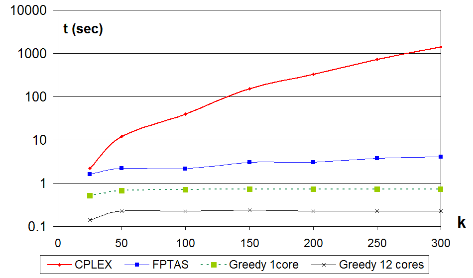
Figure 1: CPU time as function of $k$ on grid graph, $a=6$, $b=8$. Demands generated in mode II.

Instances With Real-Life Structure.

Instances 1-7 have a greater range of graph sizes and a much greater number of commodities compared to the instances with grid graphs (see Tables 1 and 2).

The LP model based on the time-expanded network required prohibitive amount of time and memory. Therefore in the case of Instances 1-7 we could compute only an upper bound $UB$ using the LP CPLEX solver. Still, in the case of Instance 1, CPLEX was unable to find an upper bound due to lack of memory and $UB$ was set to the total value of demands.

Table 3 shows the a posteriori pessimistic estimates of approximations $\omega^{\prime}$ attained by the algorithms and the corresponding CPU times (in seconds). Here FPTAS always has a greater precision than Greedy and the latter one is up to $10^{3}$ times faster even in the sequential version. Note that

Table 3: A posteriori estimated approximation $\omega^{\prime}$ and CPU times on instances with real-life structure. Here $w=0.2,L=9$.

Inst-	Greedy			FPTAS		CPLEX
ance	heuristic					computing $UB$
	CPU time		$\omega^{\prime}$	CPU time	$\omega^{\prime}$	CPU time
	1 core	12 cores
1	1.63	0.4	0.108	1689.6	0.004	–
2	0.51	0.16	0.072	157.6	0.008	7 971
3	0.28	0.1	0.094	160.4	0.01	6 947
4	0.15	0.09	0.081	80.6	0.012	1 852
5	0.11	0.06	0.094	83.6	0.012	1 872
6	0.28	0.1	0.117	3.8	0.12	345
7	0.26	0.11	0.109	389.5	0.006	144 456

In order to evaluate the algorithms on a variety of different real-life instances with similar structure we generated 300 versions of graph $G$ that model SDSN analogously to Instance 7 but in different time-frames. Different satellite positions in these time-frames lead to different links between satellites and between satellites and ground stations. The bandwidth of the links varies as well. The specification of demands remained unchanged. Application of FPTAS and Greedy to these instances in the single-core version and the same parameters as in Table 3 gave the results shown in Tables 4 and 5. The average and maximum CPU times and $\omega^{\prime}$ estimates are close to those reported in Table 3 for Instance 7, which implies that both algorithms have a stable behavior on the input data that we considered.

Table 4: CPU times (sec.) on 300 instances with real-life structure, $L=9$

	Greedy	FPTAS
		$\omega=0.4$	$\omega=0.2$	$\omega=0.1$
Average	0.3	164.8	402.0	857.6
Maximum	0.38	177.6	444.1	888.7

Table 5: A posteriori estimated approximation $\omega^{\prime}$ on 300 instances with real-life structure, $L=9$

	Greedy	FPTAS
		$\omega=0.4$	$\omega=0.2$	$\omega=0.1$
Average	0.061	0.006	0.004	0.003
Maximum	0.148	0.01	0.006	0.004

Conclusions

The proposed FPTAS has a lower time complexity bound compared to the previously known algorithms designed for a problem with the length functions of more general form.

The FPTAS and Greedy heuristic proposed in this paper are significantly faster than the CPLEX LP solver, especially on the instances with large networks and great numbers of demands. The FPTAS is more accurate but requires more CPU time than Greedy which may be a decisive factor in practical applications. Implementation of the FPTAS (hopefully) may be improved using line search for updating the current primal and dual solutions as proposed in [1] and by the means of parallel computations.

The exact LP-model discussed in Section 2 is based on a Kirchoff-type formulation in an extended graph. The alternative column generation approach has no polynomial time-bound but is often more efficient in practice. Further research might include a comparison of the algorithms presented here to the column generation method, assuming that columns are the length-bounded paths.

Appendix

Correctness of Algorithm 1 and its time complexity are established analogously to those of $(1-\omega)$-approximation algorithm for maximum MCF [6]. Before the proof of Theorem 1 we formulate and prove two lemmas. The reason why these proofs were omited in the paper is because they almost literally repeat the corresponding proofs in [6].

Lemma 1

Algorithm 1 terminates after $O\left(m\log_{1+\varepsilon}\frac{1+\varepsilon}{\delta}\right)$ augmentations.

Proof. At start, $\ell(e)=\delta$ for all edges $e$. The last time the length of an edge is updated, it is on a path of length less than one, and it is increased by at most a factor of $1+\varepsilon$. Thus the final length of any edge is at most $1+\varepsilon$. Since every augmentation increases the length of some edge by a factor of at least $1+\varepsilon$, the number of possible augmentations is at most $m\log_{1+\varepsilon}\frac{1+\varepsilon}{\delta}$. $\Box$

Lemma 2

The flow $f(e)=\sum_{P\in{\mathcal{P}}(L):e\in P}x(P),\ e\in E$ obtained by Algorithm 1 satisfies the constraints ${f(e)\leq u(e)}$ for all $e\in E$.

Proof. Every time the total flow on an edge $e$ increases by a fraction $0<a_{j}\leq 1$ of $u(e)/\log_{1+\varepsilon}\frac{1+\varepsilon}{\delta}$, its length is multiplied by $1+a_{j}\varepsilon$. Since $1+a\varepsilon\geq(1+\varepsilon)^{a}$ for all $0\leq a\leq 1,$ we have $\Pi_{j}(1+a_{j}\varepsilon)\geq(1+\varepsilon)^{\sum_{j}a_{j}}$, when $0\leq a_{j}\leq 1$ for all $j$. Thus, every time the flow on an edge increases by its capacity divided by $\log_{1+\varepsilon}\frac{1+\varepsilon}{\delta}$, the length of the edge increases by a factor of at least $1+\varepsilon$. Initially $\ell(e)=\delta$ and at the end $\ell(e)<1+\varepsilon$, so the total flow on edge $e$ cannot exceed $u(e)$. $\Box$

Theorem 1

(i) Algorithm 1 completes after $O\left(m\log_{1+\varepsilon}\frac{1+\varepsilon}{\delta}\right)$ augmentations.

(ii) Given $\delta=\frac{1+\varepsilon}{\sqrt[\varepsilon]{(1+\varepsilon)L}},$ the feasible solution to LBMCF1 problem with unbounded demands found by Algorithm 1 has a total flow value $g\geq\frac{f^{*}(1-\varepsilon)^{2}}{1+\varepsilon}.$

Proof. Part (i) follows from Lemma 1.

Now consider part (ii). Let $\ell_{j}$ denote the length function after $j$-th augmentation in Algorithm 1 and let $\alpha(\ell)$ denote the length of a shortest path in ${\mathcal{P}}(L)$ w.r.t. a length function $\ell$. Given a length function $\ell$, define $D(\ell):=\sum_{e}\ell(e)u(e),$ and let $D(j):=D(\ell_{j}).$ Then $D(j)$ is the dual objective function value corresponding to $\ell_{j}$ and $\beta:=\min_{\ell}D(\ell)/\alpha(\ell)$ is the optimal dual objective value. Let $g_{j}$ be the primal objective function value after $j$-th augmentation and let $P$ be the augmenting path. Denote $\sigma:=\log_{1+\varepsilon}\frac{1+\varepsilon}{\delta}$. Then for each $j\geq 1$,

$$D(j)=\sum_{e}\ell_{j}(e)u(e)=\sum_{e}\ell_{j-1}(e)u(e)+\varepsilon\sum_{e\in P}\ell_{j-1}(e)u$$

$$\leq D(j-1)+\varepsilon(g_{j}-g_{j-1})(1+\varepsilon)\sigma\alpha(\ell_{j-1}),$$

which implies that

$$D(j)\leq D(0)+\varepsilon(1+\varepsilon)\sigma\sum_{j^{\prime}=1}^{j}(g_{j^{\prime}}-g_{j^{\prime}-1})\alpha(\ell_{j^{\prime}-1}).$$ (16)

Consider the length function $\ell_{j}-\ell_{0}$. Note that $D(\ell_{j}-\ell_{0})=D(j)-D(0)$. For any path used by the algorithm, the length of the path using $\ell_{j}$ versus $\ell_{j}-\ell_{0}$ differs by at most $\delta L$. Since this holds for the shortest path using length function $\ell_{j}-\ell_{0}$, we have $\alpha(\ell_{j}-\ell_{0})\geq\alpha(\ell_{j})-\delta L.$ Hence

$$\beta\leq\frac{D(\ell_{j}-\ell_{0})}{\alpha(\ell_{j}-\ell_{0})}\leq\frac{D(j)-D(0)}{\alpha(\ell_{j})-\delta L}.$$

Using the bound on $D(j)-D(0)$ from equation (16), we obtain

$$\alpha(\ell_{j})\leq\delta L+\frac{\varepsilon(1+\varepsilon)\sigma}{\beta}\sum_{j^{\prime}=1}^{j}(g_{j^{\prime}}-g_{j^{\prime}-1})\alpha(\ell_{j^{\prime}-1}).$$

Observe that, for fixed $j$, this right hand side is a non-decreasing function on $\alpha(\ell_{0}),\dots,\alpha(\ell_{j-1}).$ So, for any sequence of upper bounds $\alpha^{\prime}_{j},\ j=1,\dots,$ on $\alpha(\ell_{j}),\ j=1,\dots,$ we have

$$\alpha(\ell_{j})\leq\alpha^{\prime}_{j}=\alpha^{\prime}_{j-1}(1+\varepsilon(1+\varepsilon)\sigma(g_{j}-g_{j-1})/\beta)\leq\alpha^{\prime}_{j-1}e^{\varepsilon(1+\varepsilon)\sigma(g_{j}-g_{j-1})/\beta},$$

where the last inequality uses the fact that $1+a\leq e^{a}$ for $a\geq 0$. We can use a valid upper bound $\alpha^{\prime}_{0}=\delta L$, which implies

$$\alpha(\ell_{j})\leq\delta Le^{\varepsilon(1+\varepsilon)\sigma g_{j}/\beta}.$$

By the stopping condition, after the last augmentation (let it be the augmentation number $t$) we have

$$1\leq\alpha(\ell_{t})\leq\delta Le^{\varepsilon(1+\varepsilon)\sigma g_{t}/\beta}$$

and hence

$$\frac{g_{t}}{\beta}\geq\frac{\ln(\delta L)^{-1}}{\varepsilon(1+\varepsilon)\sigma}=\frac{\ln(1+\varepsilon)\ln(L\delta)^{-1}}{\varepsilon(1+\varepsilon)\ln\frac{1+\varepsilon}{\delta}}.$$

Recalling that $\delta=\frac{1+\varepsilon}{\sqrt[\varepsilon]{(1+\varepsilon)L}}$ we obtain

$$\frac{g_{t}}{\beta}\geq\frac{(1-\varepsilon)\ln(1+\varepsilon)}{\varepsilon(1+\varepsilon)}\geq\frac{(1-\varepsilon)(\varepsilon-\varepsilon^{2}/2)}{\varepsilon(1+\varepsilon)}\geq\frac{(1-\varepsilon)^{2}}{1+\varepsilon}.$$

$\Box$

References

- [1] Albrecht, Ch.: Global routing by new approximation algorithms for multicommodity flow. IEEE Transactions on Computer-Aided Design of Integrated Circuits and Systems. 20(5) 622 – 632 (2001)
- [2] Baier, G.: Flows with Path Restrictions. Ph.D. Dissertation, TU Berlin, Berlin (2003)
- [3] Ben-Ameur, W.: Constrained-length connectivity and survivable networks, Networks 36(1) 170–33 (2000)
- [4] Baier, G., Erlebach, T., Hall, A., Köhler, E. Kolman, P., Pangrác, O., Schilling, H. and Skutella, M.: Length-bounded cuts and flows. ACM Trans. Algorithms, 7(1), 4:1–4:27 (2010)
- [5] Chaudhuri, K., Papadimitriou, C., Rao, S.: Optimum routing with quality of service constraints. Unpublished manuscript (2004).
- [6] Fleischer L.K.: Approximating fractional multicommodity flow independent of the number of commodities, SIAM J.Disc.Math., 13, 505 – 520 (2000)
- [7] Garg, N., Könemann, J.: Faster and simpler algorithms for multicommodity flow and other fractional packing problems. In: Proc. 39th IEEE Symposium on Foundations of Computer Science, FOCS’98, pp. 300–309. IEEE CS Press (1998)
- [8] Goldberg, A.V., Oldham, A.D., Plotkin, S., Stein, C.: An implementation of an approximation algorithm for minimum-cost multicommodity flows. In: Proc. of 6-th Integer Programming and Combinatorial Optimization, LNCS vol. 1412, pp. 338-352, Berlin, Springer (1998)
- [9] Garg N., Vazirani V., Yannakakis M. Primal-dual approximation algorithms for integral flow and multicut in trees, Algorithmica, 18, 3–20 (1997)
- [10] Guruswami, V., Khanna, S., Rajaraman, R., Shepherd, B., and Yannakakis, M.: Near-optimal hardness results and approximation algorithms for edge-disjoint paths and related problems. In Proceedings of the 31st Annual ACM Symposium on Theory of Computing, pages 19–28 (1999)
- [11] Hu, T.C.: Integer Programming and Network Flows. Reading, MA, Addison-Wesley Publishing Company (1970)
- [12] Kolman, P., Scheideler, C.: Improved bounds for the unsplittable flow problem. J. Algor., 61 (1), 20–44 (2006)
- [13] Nemhauser, G.L. and Wolsey, L.A.: Integer and Combinatorial Optimization. Wiley-Interscience. New York, NY (1988)
- [14] Van Mieghem, P., Kuipers, F.A., Korkmaz, T., Krunz, M., Curado, M., Monteiro, E., Masip-Bruin, X., Sole-Pareta, J., Sanchez-Lopez, S.: Quality of service routing. In: Quality of Future Internet Services. Lecture Notes in Computer Science, vol. 2856, pp. 80–117. Springer, Berlin (2003)
- [15] Schrijver, A. Combinatorial Optimization. Polyhedra and Efficiency. Vol. C. Springer, 2003.
- [16] Tang, Z., Zhao, B., Yu, W., Feng, Z and Wu, C. Software defined satellite networks: Benefits and challenges. In: Proc. of Computing, Communications and IT Applications Conference (ComComAp), pp. 127-132. IEEE (2014)
- [17] Tardos, E.: A strongly polynomial algorithm to solve combinatorial linear programs. Operations Research, 34 (2), 250-256 (1986)
- [18] Tsaggouris, G. and Zaroliagis, C.: Multiobjective optimization: Improved FPTAS for shortest paths and non-linear objectives with applications. Theory of Computing Systems, 45 (1) 162–186 (2009)