Streaming kernel regression with provably adaptive
mean, variance, and regularization

Abstract

We consider the problem of streaming kernel regression, when the observations arrive sequentially and the goal is to recover the underlying mean function, assumed to belong to an RKHS. The variance of the noise is not assumed to be known. In this context, we tackle the problem of tuning the regularization parameter adaptively at each time step, while maintaining tight confidence bounds estimates on the value of the mean function at each point. To this end, we first generalize existing results for finite-dimensional linear regression with fixed regularization and known variance to the kernel setup with a regularization parameter allowed to be a measurable function of past observations. Then, using appropriate self-normalized inequalities we build upper and lower bound estimates for the variance, leading to Bersntein-like concentration bounds. The later is used in order to define the adaptive regularization. The bounds resulting from our technique are valid uniformly over all observation points and all time steps, and are compared against the literature with numerical experiments. Finally, the potential of these tools is illustrated by an application to kernelized bandits, where we revisit the Kernel UCB and Kernel Thompson Sampling procedures, and show the benefits of the novel adaptive kernel tuning strategy.

Keywords: kernel, regression, online learning, adaptive tuning, bandits

1 Introduction

Many applications require solving an online optimization problem for an unknown, noisy, function defined over a possibly large domain space. Kernel regression methods can learn such possibly non-linear functions by sharing information gathered across observations. These techniques are being used in many fields where they serve a variety of applications like hyperparameters optimization (Snoek et al., 2012), active preference learning (Brochu et al., 2008), and reinforcement learning (Marchant and Ramos, 2014; Wilson et al., 2014). The idea is generally to rely on kernel regression to estimate a function that can be used for decision making and selecting the next observation point. Algorithmically speaking, standard kernel regression involves a regularization parameter that accounts for both the complexity of the unknown target function, and the variance of the noise. While most theoretical approaches rely on a fixed regularization parameter, in practice, people have often used heuristics in order to tune this parameter adaptively with time.

This however comes at the price of loosing theoretical guarantees. Indeed, in order for theoretical guarantees (based on concentration inequalities) to hold, existing approaches (Srinivas et al., 2010; Valko et al., 2013) require the regularization parameter in the kernel regression to be a fixed quantity. Further, they assume a prior and tight knowledge of the variance of the noise, which is unrealistic in practice. The reason for this cumbersome assumption is to adjust the regularization parameter in the kernel regression based on this deterministic quantity, as such a choice of regularization conveys a natural Bayesian interpretation (Rasmussen and Williams, 2006). Following this intuition, given an empirical estimate of the function noise based on gathered observations, one should be able to tune the regularization automatically. This is however non-trivial, first due to the streaming nature of the data, that allows the noise to be a measurable function of the past observations, second because concentration bounds on the empirical variance are currently unknown in such a general kernel setup, and finally because all existing theoretical bounds require the regularization parameter to be a deterministic constant, while we require here a parameterization that explicitly depends on past observations. The goal of this work is to provide the rigorous tools for performing an online tuning of the kernel regularization while preserving theoretical guarantees and confidence intervals in the context of streaming kernel regression with unknown noise. We thus hope to provide a sound method for adaptive tuning that is both interesting from a practical perspective and retains theoretical guarantees.

We gently start our contributions by Theorem 2.1 that generalizes existing concentration results (such as in Abbasi-Yadkori et al. (2011); Wang and de Freitas (2014)), and is explicitly stated for a regularization parameter that may differ from the noise. This result paves the way to an even more general result (Theorem 2.2) that holds when the regularization is tuned online at each step. Afterwards, we introduce a streaming variance estimator (Theorem 3.1) that yields empirical upper- and lower-bounds on the function noise. Plugging-in the resulting estimates leads to empirical Bernstein-like concentration results (Corollary 3.1) for the kernel regression, where we use the variance estimates in order to tune the regularization parameter. Section 4 presents an application to kernelized bandits, where regret bounds for Kernel UCB and Kernel Thompson Sampling procedures are derived. Section 5 discusses our results and compares them against other approaches. Finally, Section 6 shows the potential of all the previously introduced results while comparing them to existing alternatives through different numerical experiments. We postpone most of the proofs to the appendix.

2 Kernel streaming regression with a predictable noise process

Let us consider a sequential regression problem. At each time step $t\in\mathbb{N}$, a learner picks a point $x_{t}\in\mathcal{X}$ and gets the observation

$$y_{t}=f_{\star}(x_{t})+\xi_{t}\,,$$

where $f_{\star}$ is an unknown function assumed to belong to some function space $\mathcal{F}$, and $\xi_{t}$ is a random noise. We assume the process generating the observations is predictable in the sense that there is a filtration $\mathcal{H}=(\mathcal{H}_{t})_{t\in\mathbb{N}}$ such that $x_{t}$ is $\mathcal{H}_{t-1}$-measurable and $y_{t}$ is $\mathcal{H}_{t}$-measurable. Such an example is given by $\mathcal{H}_{t}=\sigma(x_{1},\dots,x_{t+1},y_{1},\dots,y_{t})$. In the sub-Gaussian streaming predictable model, we assume that for some non-negative constant $\sigma^{2}$ the following holds

$$\forall t\in\mathbb{N},\forall\gamma\in\mathbb{R},\quad\ln\mathbb{E}\Big{[}\exp(\gamma\xi_{t})\Big{|}\mathcal{H}_{t-1}\Big{]}\leqslant\frac{\gamma^{2}\sigma^{2}}{2}\,.$$

Let $k:\mathcal{X}\times\mathcal{X}\to\mathbb{R}$ be a kernel function (that is continuous, symmetric positive definite) on a compact set $\mathcal{X}$ equipped with a positive finite Borel measure, and denote $\mathcal{K}$ the corresponding RKHS. We first provide a result bounding the prediction error of a standard regularized kernel estimate, where the regularization is given by a fixed parameter $\lambda>0$.

Theorem 2.1 (Streaming Kernel Least-Squares)

Assume we are in the sub-Gaussian streaming predictable model. For a parameter $\lambda\in\mathbb{R}$, let us define the posterior mean and variances after observing $Y_{t}=(y_{1},\dots,y_{t})^{\top}\in\mathbb{R}^{t\times 1}$ as

$$\begin{cases}f_{\lambda,t}(x)=&k_{t}(x)^{\top}({\bf K}_{t}+\lambda I_{t})^{-1}Y_{t}\\ s_{\lambda,t}^{2}(x)=&\frac{\sigma^{2}}{\lambda}k_{\lambda,t}(x,x)\,\,\text{with }k_{\lambda,t}(x,x)=k(x,x)-k_{t}(x)^{\top}({\bf K}_{t}+\lambda I_{t})^{-1}k_{t}(x)\,.\end{cases}$$

where $k_{t}(x)=(k(x,x_{t^{\prime}}))_{t^{\prime}\leqslant t}$ is a $t\times 1$ (column) vector and ${\bf K}_{t}=(k(x_{s},x_{s^{\prime}}))_{s,s^{\prime}\leqslant t}$. Then $\forall\delta\!\in\![0,1]$, with probability higher than $1\!-\!\delta$, it holds simultaneously over all $x\!\in\!\mathcal{X}$ and $t\!\geqslant\!0$,

$$|f_{\star}(x)\!-\!f_{\lambda,t}(x)|\!\leqslant\!\sqrt{\frac{k_{\lambda,t}(x,x)}{\lambda}}\bigg{[}\!\sqrt{\lambda}\|f_{\star}\|_{\mathcal{K}}\!+\!\sigma\sqrt{2\ln(1/\delta)+2\gamma_{t}(\lambda)}\bigg{]}\,,$$

where the quantity $\quad\gamma_{t}(\lambda)=\frac{1}{2}\sum_{t^{\prime}=1}^{t}\!\ln\!\Big{(}\!1\!+\!\frac{1}{\lambda}k_{\lambda,t^{\prime}-1}(x_{t^{\prime}},x_{t^{\prime}})\Big{)}\quad$ is the information gain.

Remark 2.1

This result should be considered as an extension of (Abbasi-Yadkori et al., 2011, Theorem 2) from finite-dimensional to possibly infinite dimensional function space. It is a non-trivial result as the Laplace method must be amended in order to be applied.

Remark 2.2

This result holds uniformly over all $x\in\mathcal{X}$ and most importantly over all $t\geqslant 0$, thanks to a random stopping time construction (related to the occurrence of bad events) and a self-normalized inequality handling this stopping time. This is in contrast with results such as Wang and de Freitas (2014), that are only stated separately for each $t$.

Remark 2.3

The quantity $\gamma_{t}(\lambda)$ directly generalizes the classical notion of information gain (Cover and Thomas, 1991), that is recovered for the choice of regularization $\lambda=\sigma^{2}$.

The case when $\lambda=\lambda^{\star}\stackrel{{\scriptstyle\rm def}}{{=}}\sigma^{2}/\|f\|_{\mathcal{K}}^{2}$ is of special interest, since we get on the one hand

$$f_{t}^{\star}(x) = k_{t}(x)^{\top}({\bf K_{t}}+\lambda^{\star}I_{t})^{-1}Y_{t}$$

$$s_{t}^{2\star}(x) = \|f\|_{\mathcal{K}}^{2}k_{t}(x,x)\,\,\text{with }k_{t}(x,x)=k(x,x)-k_{t}(x)^{\top}({\bf K_{t}}+\lambda^{\star}I_{t})^{-1}k_{t}(x)$$

and on the other hand $\|f\|_{\mathcal{K}}k_{t}(x,x)^{1/2}\Big{[}1+\sqrt{2\ln(1/\delta)+2\gamma_{t}(\lambda^{\star})}\Big{]}$. In practice however, neither $\|f\|_{\mathcal{K}}^{2}$ nor $\sigma^{2}$ may be known exactly. In this paper, we assume that an upper bound $C$ is given on $\|f\|_{\mathcal{K}}$. Then, we want to build an estimate of $\sigma^{2}$ at each time $t$ in order to tune $\lambda$. Using a sequence of regularization parameters $(\lambda_{t})_{t\geqslant 1}$ that is tuned adaptively based on the past observations requires to modify the previous theorem (it is only valid for a deterministic $\lambda$) into the following more general statement:

Theorem 2.2 (Streaming Kernel Least-Squares with online tuning)

Under the same assumption as Theorem 2.1, let $\bm{\lambda}=(\lambda_{t})_{t\geqslant 1}$ be a predictable positive sequence of parameters, that is $\lambda_{t}$ is $\mathcal{H}_{t-1}$-measurable for each $t$. Assume that for each $t$, $\lambda_{t}\geqslant\lambda_{\star}$ holds for a positive constant $\lambda_{\star}$. Let us define the modified posterior mean and variances after observing $Y_{t}\in\mathbb{R}^{t}$ as

$$\begin{cases}f_{\bm{\lambda},t}(x)\!\!&=k_{t}(x)^{\top}({\bf K}_{t}+\lambda_{t+1}I_{t})^{-1}Y_{t}\\ s_{\bm{\lambda},t}^{2}(x)\!\!&=\frac{\sigma^{2}}{\lambda_{t+1}}k_{\lambda_{t+1},t}(x,x)\,\,\text{with }k_{\lambda,t}(x,x)\!=\!k(x,x)\!-\!k_{t}(x)^{\top}\!({\bf K}_{t}+\lambda I_{t})^{-1}k_{t}(x)\,,\end{cases}$$

where $k_{t}(x)\!=\!(k(x,x_{t^{\prime}}))_{t^{\prime}\leqslant t}$, and ${\bf K}_{t}\!=\!(K(x_{s},x_{s^{\prime}}))_{s,s^{\prime}\leqslant t}$. Then for all $\delta\!\in\![0,1]$, with probability higher than $1-\delta$, it holds simultaneously over all $x\in\mathcal{X}$ and $t\geqslant 0$

$$|\!f_{\star}(x)\!-\!f_{\bm{\lambda},t}(x)|\!\leqslant\!\sqrt{\frac{k_{\lambda_{t+1},t}(x,x)}{\lambda_{t+1}}}\Big{[}\!\sqrt{\!\lambda_{t\!+\!1}}\|f_{\star}\|_{\mathcal{K}}\!+\!\sigma\sqrt{2\ln(\!1/\delta)\!+\!2\gamma_{t}(\lambda_{\star})}\Big{]}\,.$$

The proof is presented in Appendix A.

The regularization parameter $\lambda_{t+1}$ is therefore used in conjunction with previous data up to time $t$ to provide the posterior regression model (mean and variance) that is used in return to acquire the next observation $y_{t+1}$ on point $x_{t+1}$.

Remark 2.4

Since $\lambda_{t}$ is allowed to be $\mathcal{H}_{t-1}$-measurable, this gives theoretical guarantees for virtually any adaptive tuning procedure of the regularization parameter.

Remark 2.5

The assumption that $\lambda_{t}\geqslant\lambda_{\star}$ will be naturally satisfied for the choice of regularization we consider.

3 Variance estimation

We now focus on the estimation of the variance parameter of the noise in the case when it is unknown, or loosely known. Theorem 2.2 suggests to define the sequence $(\lambda_{t})_{t\geqslant 1}$ by

$$\lambda_{t}=\sigma_{+,t-1}^{2}/C^{2}\quad\text{with}\quad\sigma_{+,t}=\min\{\tilde{\sigma}_{+,t},\sigma_{+,t-1}\}\quad\text{and}\quad\sigma_{+,0}=\sigma_{+}\,,$$ (1)

where $\sigma_{+}\geqslant\sigma$ is an initial loose upper bound on $\sigma$ and $\tilde{\sigma}_{+,t}$ is an upper-bound estimate on $\sigma$ built from all observations gathered up to time $t$ (inclusively). This ensures that $\lambda_{t}$ is $\mathcal{H}_{t-1}$ measurable for all $t$ and satisfies $\lambda_{t}\geqslant\lambda_{\star}$ with high probability, where $\lambda_{\star}=\sigma^{2}/C^{2}$. The crux is now to define the upper-bound estimate $\sigma_{+,t}$ on $\sigma$. In order to get a variance estimate, one obviously requires more than the sub-Gaussian assumption, since the term $\sigma^{2}$ has no reason to be tight (the inequality remains valid when $\sigma^{2}$ is replaced with any larger value). In order to convey the minimality of $\sigma^{2}$, we assume that the noise sequence is both $\sigma$-sub-Gaussian and second-order $\sigma$-sub-Gaussian, in the sense that

$$\forall t,\forall\gamma<\frac{1}{2\sigma^{2}}\quad\ln\mathbb{E}\bigg{[}\exp(\gamma\xi_{t}^{2})\bigg{|}\mathcal{H}_{t-1}\bigg{]}\leqslant-\frac{1}{2}\ln\Big{(}1-2\gamma\sigma^{2}\Big{)}\,.$$

Remark 3.1

To avoid any technicality, one may assume that $\xi_{t}|\mathcal{H}_{t-1}$ is exactly $\mathcal{N}(0,\sigma^{2})$, in which case it is trivially second-order $\sigma$-sub-Gaussian.

Now let $\quad\widehat{\sigma}^{2}_{\lambda,T}=\frac{1}{T}\sum_{t=1}^{T}(y_{t}-f_{\lambda,T}(x_{t}))^{2}\quad$ denote the (slightly biased) variance estimate for a regularization parameter $\lambda$.

Theorem 3.1 (Streaming Kernel variance estimate)

Assume we are in the predictable second-order $\sigma$-sub-Gaussian streaming regression model, with a predictable positive sequence $\bm{\lambda}$ such that $\lambda_{t}\geqslant\lambda_{\star}$ holds for all $t$. Let us introduce the following quantities

$$C_{t}(\delta)=\ln(e/\delta)\big{[}1+\ln(\pi^{2}\ln(t)/6)/\ln(1/\delta)\big{]},\qquad D_{\lambda,t}(\delta)=2\ln(1/\delta)+2\gamma_{t}(\lambda)$$

$$\text{ and finally}\quad\alpha=\max\Big{(}1-\sqrt{\frac{C_{t}(\delta^{\prime})}{t}}-\sqrt{\frac{C_{t}(\delta^{\prime})+2D_{\lambda_{\star},t}(\delta^{\prime})}{t}},0\Big{)}\,.$$

Then, let us introduce the following variance bounds, defined differently depending on whether a deterministic upper bound $\sigma_{+}\geqslant\sigma$ is known (case 1) or not (case 2).

$$\sigma_{+,t}(\lambda,\lambda_{\star})=\begin{cases}\widehat{\sigma}_{\lambda,t}+\sigma_{+}\bigg{(}\sqrt{\frac{C_{t}(\delta^{\prime})}{t}}+\sqrt{\frac{C_{t}(\delta^{\prime})+2D_{\lambda_{\star},t}(\delta^{\prime})}{t}}\bigg{)}+\sqrt{\frac{2\sigma_{+}\lVert f_{\star}\rVert_{\mathcal{K}}\sqrt{\lambda D_{\lambda_{\star},t}(\delta^{\prime})}}{t}}&\text{(case 1)}\\ \frac{1}{\alpha^{2}}\Bigg{(}\sqrt{\widehat{\sigma}_{\lambda,t}\alpha+\frac{\lVert f_{\star}\rVert_{\mathcal{K}}\sqrt{\lambda D_{\lambda_{\star},t}(\delta^{\prime})}}{2t}}+\sqrt{\frac{\lVert f_{\star}\rVert_{\mathcal{K}}\sqrt{\lambda D_{\lambda_{\star},t}(\delta^{\prime})}}{2t}}\Bigg{)}^{2}&\text{(case 2)}\end{cases}$$

$$\sigma_{-,t}(\lambda)=\begin{cases}\widehat{\sigma}_{\lambda,t}-\sigma_{+}\sqrt{\frac{2C_{t}(\delta^{\prime})}{t}}-\lVert f_{\star}\rVert_{\mathcal{K}}\sqrt{\frac{\lambda}{t}\bigg{(}1-\frac{1}{\max_{t^{\prime}\leqslant t}(1+\frac{1}{\lambda}k_{\lambda,t^{\prime}-1}(x_{t^{\prime}},x_{t^{\prime}}))}\bigg{)}}&\text{(case 1)}\\ \bigg{[}\widehat{\sigma}_{\lambda,t}-\lVert f_{\star}\rVert_{\mathcal{K}}\sqrt{\frac{\lambda}{t}\bigg{(}1-\frac{1}{\max_{t^{\prime}\leqslant t}(1+\frac{1}{\lambda}k_{\lambda,t^{\prime}-1}(x_{t^{\prime}},x_{t^{\prime}}))}\bigg{)}}\bigg{]}\bigg{(}1+\sqrt{\frac{2C_{t}(\delta^{\prime})}{t}}\bigg{)}^{-1}&\text{(case 2)}.\end{cases}$$

Then with probability higher than $1-3\delta^{\prime}$, it holds simultaneously for all $t\geqslant 0$

$$\sigma_{-,t}(\lambda_{t})\leqslant\sigma\leqslant\sigma_{+,t}(\lambda_{t},\lambda_{\star})\,.$$

The proof is presented in Appendix B.

Remark 3.2

The case when absolutely no bound is known on the noise $\sigma^{2}$ is challenging in practice. In this case, it is intuitive that one should not be able to recover the noise with too few samples. The bound stated in Theorem 3.1 (see Appendix B) supports this intuition, as when the number of observations is too small, then $\alpha=0$ and the corresponding bound becomes trivial ($\sigma\leqslant\infty$).

Remark 3.3

In the variance bounds of Theorem B.1 the term $\|f_{\star}\|_{\mathcal{K}}$ appears systematically with the factor $\sqrt{\lambda}$. This suggests we need to choose $\lambda$ proportional to $1/\|f_{\star}\|_{\mathcal{K}}^{2}$, which gives further justification to the target $\lambda_{\star}=\sigma^{2}/C^{2}$, where $C$ is a known upper bound on $\|f_{\star}\|$.

Remark 3.4

In practice, we advice to choose the best of case 1 and case 2 bounds when $\sigma_{+}\geqslant\sigma$ is known.

In order to estimate the upper bound $\sigma_{+,t}(\lambda,\lambda_{\star})$, one needs at least a lower-bound on $\lambda_{\star}$. Let us define

$$\sigma_{-,t}=\max\{\tilde{\sigma}_{-,t},\sigma_{-,t-1}\}\quad\text{with}\quad\sigma_{-,0}=\sigma_{-}\,,$$ (2)

where $0\leqslant\sigma_{-}\leqslant\sigma$ is a initial lower-bound on $\sigma$ and $\tilde{\sigma}_{-,t}$ is a lower-bound estimate on $\sigma$ built from all observations gathered up to time $t$ (inclusively). Then, one way to proceed is, at each time step $t\geqslant 1$, to build an estimate $\tilde{\sigma}_{-,t}=\sigma_{-,t}(\lambda)$, which in return can be used to compute the lower quantity $\lambda_{-}\leqslant\lambda_{\star}$, and obtain the estimate $\tilde{\sigma}_{+,t}=\sigma_{+,t}(\lambda,\lambda_{-})\geqslant\sigma_{+,t}(\lambda,\lambda_{\star})$. Then, we compute the predictable sequence $\bm{\lambda}$ as described by equation 1. Further replacing the variance $\sigma$ with its estimate $\sigma_{+,t}$ using a union bound in the result of Theorem 2.2, we derive confidence bounds that are fully computable in the context where the regularization parameter is adaptively tuned and the function noise is unknown. This is summarized in the following empirical Bernstein-style inequality:

Corollary 3.1 (Kernel empirical-Bernstein inequality)

Assume that $C\geqslant\|f\|_{\mathcal{K}}$. Let us define the following noise lower-bound for each $t\geqslant 1$

$$\sigma_{-,t}=\max\{\sigma_{-,t}(\lambda_{t-1}),\sigma_{-,t-1}\}$$

and define $\lambda_{-}=\sigma^{2}_{-,t}/C^{2}$ as the corresponding lower bound on $\lambda_{\star}$. Then, let us define the following noise upper bound for each $t\geqslant 1$

$$\sigma_{+,t}\!=\!\min\{\sigma_{+,t}(\lambda_{t-1},\lambda_{-}),\sigma_{+,t-1}\}\,.$$

Define the regularization parameterizing the regression model used for acquiring observation at time $t$ to be $\lambda_{t}=\sigma_{+,t}^{2}/C^{2}$, according to Equation 1. Then with probability higher than $1-4\delta$, the following is valid simultaneously for all $x\in\mathcal{X}$ and $t\geqslant 0$,

$$\big{|}\!f_{\star}(x)\!-\!f_{\lambda_{t},t}(x)\big{|}\!\leqslant\!\sqrt{\frac{k_{\lambda_{t},t}(x,x)}{\lambda_{t}}}B_{\lambda_{t},t}(\delta)\qquad\text{where}$$

$$B_{\lambda_{t},t}(\delta)=\!\sqrt{\!\lambda_{t}}C\!+\!\sigma_{+,t}\sqrt{2\ln(1/\delta)+2\gamma_{t}(\lambda_{-})}\,.$$ (3)

Remark 3.5

This result is especially interesting since it provides a fully empirical confidence envelope function around $f_{\star}$. When an initial bound on the noise $\sigma_{+}$ is known and considered to be tight, one may simply choose the constant deterministic sequence $\bm{\lambda}=(\lambda,\dots,\lambda)$, in which case the same result holds for $\lambda_{-}=\lambda$ and $\sigma_{+,t}=\sigma_{+}$.

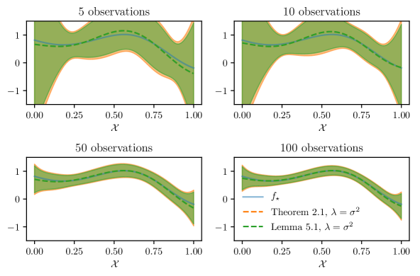
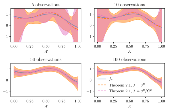
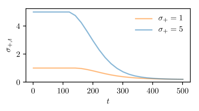
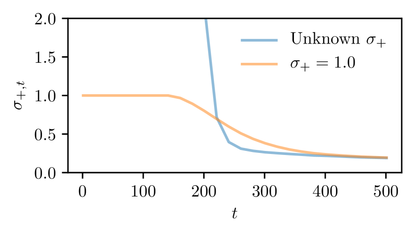
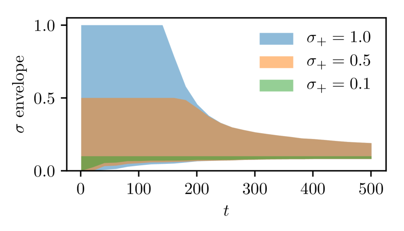
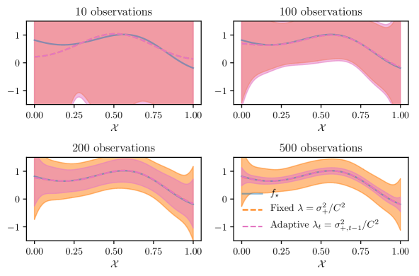
We observe from Theorem 3.1 that the tightness of the noise estimates depends on the $\lambda$ parameter that is used for computing $\tilde{\sigma}_{-,t}$ and $\tilde{\sigma}_{+,t}$. Since $\sigma^{2}/C^{2}\leqslant\lambda_{t}\leqslant\sigma_{+}^{2}/C^{2}$ holds with high probability by construction, using such an adaptive $\lambda_{t}$ should yield tighter bounds than using a fixed $\sigma_{+}^{2}/C^{2}$. This is supported by the numerical experiments of Section 6.2.

4 Application to kernelized bandits

Here is a direct application of our results in the framework of stochastic multi-armed bandits with structured arms embedded in an RKHS (Srinivas et al., 2010; Valko et al., 2013). At each time step $t\geqslant 1$, a bandit algorithm recommends a point $x_{t}$ to sample and observes a noisy outcome $y_{t}=f_{\star}(x_{t})+\xi_{t}$, where $\xi_{t}\sim\mathcal{N}(0,\sigma^{2})$. Let $\star=\mathop{\mathrm{argmax}}_{x\in{\mathbb{X}}}f_{\star}(x)$ be the optimal arm. The goal of an algorithm is to pick a sequence of points $(x_{t})_{t\leqslant T}$ that minimizes the cumulative regret

$$\mathfrak{R}_{T}=\sum_{t=1}^{T}f_{\star}(\star)-f_{\star}(x_{t}).$$ (4)

In this context, one needs to build tight confidence sets on the mean of each arm, and this will be given by Corollary 3.1. We illustrate our technique on two main bandit strategies: Upper Confidence Bound (UCB) (Auer et al., 2002) and Thompson Sampling (TS) (Thompson, 1933); both are adapted here to the kernel setting with unknown variance.

Definition 4.1 (Information gain with unknown variance)

We define the information gain at time $t$ for a regularization parameter $\lambda$ to be

$$\gamma_{t}(\lambda)=\frac{1}{2}\sum_{t^{\prime}=1}^{t}\ln\Big{(}1+\frac{1}{\lambda}k_{\lambda,t^{\prime}-1}(x_{t^{\prime}},x_{t^{\prime}})\Big{)}\,.$$

This definition directly extends the usual definition of information gain, that can be recovered by choosing $\lambda=\sigma^{2}$. The following extension of Lemma 7 in Wang and de Freitas (2014) (see also Srinivas et al. (2012)) to the case when the variance is estimated plays an important role in the regret analysis of both algorithms.

Lemma 4.1 (From sum of variances to information gain)

Let us assume that the kernel is bounded by $1$ in the sense that $\sup_{x\in\mathcal{X}}k(x,x)\leqslant 1$. Let $\bm{\lambda}$ be any sequence such that $\forall\lambda\in\bm{\lambda},\lambda\geqslant\sigma^{2}/C^{2}$. For instance, this is satisfied with high probability when using Equation 1. Then, it holds

$$\sum_{t=1}^{T}s_{\bm{\lambda},t-1}^{2}(x_{t})=\sigma^{2}\sum_{t=1}^{T}\frac{1}{\lambda_{t}}k_{\lambda_{t},t-1}(x_{t},x_{t})\leqslant\frac{2C^{2}}{\ln(1+C^{2}/\sigma^{2})}\gamma_{T}(\sigma^{2}/C^{2})\,.$$

In the sequel, it is useful to bound the confidence bound term $B_{\lambda_{t},t}(\delta)$ from Equation 3.

Lemma 4.2 (Deterministic bound on the confidence bound)

Assume that we are given a constant $0<\sigma_{-}<\sigma$, so that $\sigma_{t,-}\geqslant\sigma_{-}$ holds for all $t$. Then for all $t\leqslant T$, the confidence bound term is upper-bounded by the following deterministic quantity

$$B_{\lambda_{t},t}(\delta) \leqslant\sigma_{+}\bigg{(}1+\sqrt{2\ln(1/\delta)+2\gamma_{T}(\sigma_{-}^{2}/C^{2})}\bigg{)}\,.$$

Further, we have $\gamma_{t}(\sigma_{t,-}^{2}/C^{2})=\gamma_{t}(\sigma_{-}^{2}/C^{2})+O(1/\sqrt{t})$.

Remark 4.1

The term $\sigma_{+}$ can be replaced with a more refined term $\sigma+O(1/\sqrt{t})$ thanks to the confidence bounds on the variance estimates.

Kernel UCB with unknown variance

The upper bound on the error can be used directly in order to build a UCB-style algorithm. Formally, the vanilla UCB algorithm (Auer et al., 2002) corresponding to our setting picks at time $t$ the arm

$$x_{t}\in\mathop{\mathrm{argmax}}_{x\in\mathcal{X}}f^{+}_{\lambda_{t},t-1}(x)\quad\text{ where }\quad f^{+}_{\lambda,t}(x)=f_{\lambda,t}(x)+\sqrt{\frac{k_{\lambda,t}(x,x)}{\lambda}}B_{\lambda,t}(\delta)\,.$$ (5)

Following the regret proof strategy of Abbasi-Yadkori et al. (2011), with some minor modifications, yields the following guarantee on the regret of this strategy:

Theorem 4.1 (Kernel UCB with unknown noise and adaptive regularization)

With probability higher than $1-\delta$, the regret of Kernel UCB with adaptive regularization and variance estimation satisfies for all $T\geqslant 0$ (recall that $B_{\lambda_{t+1},t}(\delta)$ is defined in Equation 3):

$$\mathfrak{R}_{T}\leqslant 2\sum_{t=1}^{T}\sqrt{\frac{k_{\lambda_{t},t-1}(x_{t},x_{t})}{\lambda_{t}}}B_{\lambda_{t},t-1}(\delta/4)\,.$$

In particular, we have

$$\mathfrak{R}_{T} \leqslant 2\frac{\sigma_{+}}{\sigma}\Big{(}1+\sqrt{2\ln(4/\delta)+2\gamma_{T}(\sigma_{-}^{2}/C^{2})}\big{)}C\sqrt{T\frac{2\gamma_{T}(\sigma^{2}/C^{2})}{\ln(1+C^{2}/\sigma^{2})}}\,.$$

Remark 4.2

This result that holds simultaneously over all time horizon $T$ extends that of Abbasi-Yadkori et al. (2011) first to kernel regression and then to the case when the variance of the noise is unknown. This should also be compared to Valko et al. (2013) that assumes bounded observations, which implies a bounded noise (with known bound) and a bounded $f_{\star}$, and Srinivas et al. (2010) that provides looser bounds.

Kernel TS with unknown variance

Another application of our confidence bounds is in the analysis of Thompson sampling in the kernel scenario. Before presenting the result, let us say a few words about the design of TS algorithm in a kernel setting. Such an algorithm requires sampling from a posterior distribution over the arms. It is natural to consider a Gaussian posterior with posterior means and variances given by the kernel estimates. However, it has been noted in a series of papers (Agrawal and Goyal, 2014; Abeille and Lazaric, 2016) that, in order to obtain provable regret minimization guarantees, the posterior variance should be inflated (although in practice, the vanilla version without inflation may work better). Following these lines of research, and owing to our novel confidence bounds, we derive the following TS algorithm using a posterior variance inflation factor $v_{t}^{2}$.

Parameters: regularization sequence $\bm{\lambda}$, variance inflation factor $v_{t}^{2}$ for each $t$.

1:  for all $t\geqslant 1$ do

2:     compute the posterior mean $\widehat{\bf f}_{t-1}=(f_{\lambda_{t},t-1}(x))_{x\in{\mathbb{X}}}$

3:     compute the posterior covariance $\widehat{\bm{\Sigma}}_{t-1}=\frac{\sigma_{+,t-1}^{2}}{\lambda_{t}}\big{(}k_{\lambda_{t},t-1}(x,x^{\prime})\big{)}_{x,x^{\prime}\in{\mathbb{X}}}$

4:     sample $\tilde{f}_{t}=\mathcal{N}(\widehat{\bf f}_{t-1},v_{t}^{2}\widehat{\bm{\Sigma}}_{t-1})$

5:     play $x_{t}=\mathop{\mathrm{argmax}}_{x\in{\mathbb{X}}}\tilde{f}_{t}(x)$

6:     observe outcome $y_{t}=f_{\star}(x_{t})+\xi_{t}$

7:  end for

Algorithm 1 Kernel TS with adaptive variance estimation and regularization tuning

Remark 4.3

The algorithm does not know the variance $\sigma^{2}$ of the noise, but uses an upper estimate $\sigma_{+,t-1}^{2}$.

Remark 4.4

We assume that the set of arms ${\mathbb{X}}$ is discrete. This is merely for practical reasons since otherwise updating the estimate of $f_{\star}$ in a RKHS requires memory and computational times that are unbounded with $t$. This also simplifies the analysis.

The following regret bound can then be obtained after some careful but easy adaptation of Agrawal and Goyal (2014). We provide the proof of this result in Appendix C, which can be of independent interest, being a more rigorous and somewhat simpler rewriting of the original proof technique from Agrawal and Goyal (2014).

Theorem 4.2 (Regularized Kernel TS with variance estimate)

Assume that the maximal instantaneous pseudo-regret $R=\max_{x\in{\mathbb{X}}}\big{(}f_{\star}(\star)-f_{\star}(x)\big{)}$ is finite. Then, the regret of Kernel TS (Algorithm 1) with $v_{t}=\frac{B_{\lambda_{t},t-1}(\delta/4)}{\sigma_{+,t-1}}$ after $T$ episodes is $\mathcal{O}(C\sqrt{T\ln(T|{\mathbb{X}}|)}\gamma_{T}(\sigma^{2}/C^{2}))$ with probability $1-3\delta$. More precisely, with probability $1-3\delta$, the regret is bounded for all $T\geqslant 0$:

$$\mathfrak{R}_{T} \leqslant C_{1,T}\bigg{(}\sum_{t=1}^{T}\sqrt{\frac{k_{\lambda_{t},t-1}(x_{t},x_{t})}{\lambda_{t}}}B_{\lambda_{t},t-1}(\delta/4)\bigg{)}+C_{2}R\sqrt{T\ln(1/\delta)}+4\pi eR\delta\,,$$

where $C_{1,T}=(4\sqrt{\pi e}+1)\bigg{(}1+\sqrt{2\ln\Big{(}\frac{T(T+1)|{\mathbb{X}}|}{\sqrt{\pi}\delta}\Big{)}}\bigg{)}$ and $C_{2}=\sqrt{8\pi e(1+\delta\sqrt{4\pi e})^{2}}$.

Further, we have

$$\mathfrak{R}_{T} \leqslant C_{1,T}\frac{\sigma_{+}}{\sigma}\Big{(}1+\sqrt{2\ln(4/\delta)+2\gamma_{T}(\sigma_{-}^{2}/C^{2})}\Big{)}C\sqrt{T\frac{2\gamma_{T}(\sigma^{2}/C^{2})}{\ln(1+C^{2}/\sigma^{2})}}$$

$$+C_{2}R\sqrt{T\ln(1/\delta)}+4\pi eR\delta\,.$$

Remark 4.5

As our confidence intervals do not require a bounded noise, likewise we can control the regret with high probability without requiring bounded observations, contrary to earlier works such as Valko et al. (2013).

5 Discussion and related works

Concentration results

Theorem 2.1 extends the self-normalized bounds of Abbasi-Yadkori et al. (2011) from the setting of linear function spaces to that of an RKHS with sub-Gaussian noise. Based on a nontrivial adaptation of the Laplace method, it yields self-normalized inequalities in a setting of possibly infinite dimension. It generalizes the following result of Wang and de Freitas (2014) to kernel regression with $\lambda\neq\sigma^{2}$, which was already a generalization of a previous result by Srinivas et al. (2010) for bounded noise. It is also more general than the concentration result from Valko et al. (2013), for kernel regression with $\lambda\neq\sigma^{2}$, which holds under the assumption of bounded observations.

Lemma 5.1 (Proposition 1 from Wang and de Freitas (2014))

Let $f_{\star}$ denote a function in the RKHS $\mathcal{K}$ induced by kernel $k$ and let us define the posterior mean and variances with $\lambda=\sigma^{2}$, for (arbitrary) data $(x_{t^{\prime}})_{t^{\prime}\leqslant t}$. Assuming $\sigma$-sub-Gaussian noise variables, then for all $\delta^{\prime}\in(0,1)$ we have that

$$\mathbb{P}\big{[}\exists x\in\mathcal{X}:|f_{\lambda,t}(x)-f_{\star}(x)|\geqslant\ell_{\lambda,t+1}(\delta^{\prime})k_{\lambda,t}^{1/2}(x,x)\big{]}\leqslant\delta^{\prime},\quad\text{where}\quad$$

$$\ell_{\lambda,t}^{2}(\delta^{\prime})=\|f\|_{\mathcal{K}}^{2}+\sqrt{8\gamma_{t-1}(\lambda)\ln\frac{2}{\delta^{\prime}}}+\sqrt{2\ln\frac{4}{\delta^{\prime}}}\|f\|_{\mathcal{K}}+2\gamma_{t-1}(\lambda)+2\sigma\ln\frac{2}{\delta^{\prime}}$$

and $\gamma_{t}(\lambda)=\frac{1}{2}\sum_{t^{\prime}=1}^{t}\ln\big{(}1+\frac{1}{\lambda}k_{\lambda,t^{\prime}-1}(x_{t^{\prime}},x_{t^{\prime}})\big{)}$ is the information gain.

Remark 5.1

This results provides a bound that is valid for each $t$, with probability higher $1-\delta$. In contrast, results from Abbasi-Yadkori et al. (2011), as well as Theorem 2.1 hold with probability higher $1-\delta$, uniformly for all $t$, and are thus much stronger in this sense.

Theorem 2.2 extends Theorem 2.1 to the case when the regularization is tuned online based on gathered observations. To the best of our knowledge, no such result exists in the literature at the time of writing this paper. Moreover, Theorem 3.1 provides variance estimates with confidence bounds scaling with $1/\sqrt{t}$, in the spirit of the results from Maurer and Pontil (2009), that were provided in the i.i.d. case. Thus, Theorem 3.1 also appears to be new. Finally, Corollary 3.1 further specifies Theorem 2.2 to the situation where the regularization is tuned according to Theorem 3.1, yielding a fully adaptive regularization procedure with explicit confidence bounds.

Bandits optimization

When applied to the setting of multi-armed bandits, Theorems 4.2 and 4.1 respectively extend linear TS (Agrawal and Goyal, 2014; Abeille and Lazaric, 2016) and UCB (Li et al., 2010; Chu et al., 2011) to the RKHS setting. Similar extensions have been provided in the literature: GP-UCB (Srinivas et al., 2010) generalizes UCB from the linear to the RKHS setting through the use of Gaussian processes; this corresponds to the case when $\lambda=\sigma^{2}$. The bounds they provide in the case when the target function belongs to an RKHS is however quite loose. KernelUCB (Valko et al., 2013) also generalizes UCB from the linear to the RKHS setting through the use of kernel regression. However the analysis of this algorithm was out of reach of their proof technique (that requires independence between arms) and they analyze instead the arguably less appealing variant called SupKernelUCB. Also, the analysis of both GP-UCB and SupKernelUCB in the agnostic setting are respectively limited to bounded noise and bounded observations.

6 Illustrative numerical experiments

In this section, we illustrate the results introduced in the previous Sections 2 and 3 on a few examples. The first one is the concentration result on the mean from Theorem 2.1, the second one is the variance estimate from Theorem 3.1, and the last one combines the formers by using the noise estimate to tune $\lambda_{t+1}=\sigma_{t}^{2}/C^{2}$ in Theorem 2.2, which corresponds to Corollary 3.1. We finally show the performance of kernelized bandits techniques using the provided variance estimates and adaptative regularization schemes.

We conduct the experiments using the function $f_{\star}$ shown by Figure 1, which has norm $\|f_{\star}\|_{\mathcal{K}}=\|\theta_{\star}\|_{2}=2.06$ in the RKHS induced by a Gaussian kernel $\quad k(x,x^{\prime})=e^{-\frac{(x-x^{\prime})^{2}}{2\rho^{2}}}\quad$ with length scale $\rho=0.3$. We consider the space $\mathcal{X}=[0,1]$ and that the standard deviation of the noise is $\sigma=0.1$. All further experiments use the upper-bound $C=5$ on $\|f_{\star}\|_{\mathcal{K}}$ and the lower-bound $\sigma_{-}=0.01$ on $\sigma$.

Figure 1: Test function $f_{\star}$ used in the following numerical experiments.

6.1 Kernel concentration bound

The following experiments compare the concentration result given by Theorem 2.1 with the kernel concentration bounds from Wang and de Freitas (2014) reported by Lemma 5.1. The true noise $\sigma=0.1$ is assumed to be known and all observations are uniformly sampled from $\mathcal{X}$. In both cases, we use a fixed confidence level $\delta=0.1$. Figure 2 shows that for $\lambda=\sigma^{2}$, the result given by Theorem 2.1 recovers the confidence envelope of Wang and de Freitas (2014). Note however that the confidence bound that we plot for Theorem 2.1 are valid uniformly over all time steps, while the one derived from Wang and de Freitas (2014) is only valid separately for each time. Further, Theorem 2.1 generalizes the latter result to the case where $\lambda\neq\sigma^{2}$. For illustration, Figure 3 illustrates the confidence envelopes in the special case where $\lambda=\sigma^{2}/C^{2}$, which also shows the potential benefit of such a tuning.

Figure 2: Confidence interval of Theorem 2.1 and Lemma 5.1 (Wang and de Freitas, 2014).

Figure 3: Confidence interval of Theorem 2.1 for different $\lambda$.

6.2 Empirical variance estimate

We now illustrate the convergence rate of the noise estimates $\sigma_{-,t}=\max\{\sigma_{-,t}(\lambda),\sigma_{-,t-1}\}$ and $\sigma_{+,t}=\min\{\sigma_{+,t}(\lambda,\lambda_{-}),\sigma_{+,t-1}\}$ computed using Theorem 3.1, where $\lambda_{-}=\sigma_{-,t}^{2}/C^{2}$ and $\delta=0.1$. All observations are uniformly sampled from $\mathcal{X}$. Section 3 suggests that $\lambda=\sigma_{+,t-1}^{2}/C^{2}$ should provide tighter bounds than a fixed $\lambda=\sigma_{+}^{2}/C^{2}$. Figure 4 shows that this is indeed the case especially for large values of $t$. We also see that the adaptive update of $\lambda$ converges to the same value, whatever the initial bound $\sigma_{+}$. This is especially interesting when $\sigma_{+}$ is a loose initial upper bound on $\sigma$.

(a)

(b)

Figure 4: Noise estimate from Theorem 3.1 with $\sigma_{+}$ for a) fixed $\lambda=\sigma_{+}^{2}/C^{2}$; b) $\lambda=\sigma_{+,t-1}^{2}/C^{2}$.

In practice, the bound of Theorem 3.1 not using the knowledge of $\sigma_{+}$ may be useful even when $\sigma_{+}$ is known. This is illustrated by Figure 5(a) that plots the upper-bound variance estimate $\sigma_{+,t}(\lambda,\lambda_{-})$ for $\lambda=\sigma_{+,t-1}^{2}/C^{2}$ in both cases. In practice, we suggest to use the minimum of the bound using the knowledge of $\sigma_{+}$ (case 1) and of the agnostic one (case 2) to set $\sigma_{+,t}(\lambda,\lambda_{-})$ and the maximum for $\sigma_{-,t}(\lambda)$. Figure 5(b) shows the resulting noise estimate envelopes for different $\sigma_{+}$ values (recall that $\sigma=0.1$).

(a)

(b)

Figure 5: Variance estimate a) from Theorem 3.1, with and without $\sigma_{+}$; b) as minimum of the bounds and $\sigma_{+}$, for different upper-bounds.

6.3 Adaptive regularization

We now combine the previous experiments and use the estimated noise in order to tune the regularization. Recall that we consider $\sigma_{-,0}=\sigma_{-}$, $\sigma_{+,0}=\sigma_{+}$, and $\lambda_{0}=\sigma_{+}^{2}/C^{2}$. On each time $t\geqslant 1$, we estimate the noise lower-bound $\sigma_{-,t}=\max\{\sigma_{-,t}(\lambda_{t-1}),\sigma_{-,t-1}\}$ using Theorem 3.1 and set $\lambda_{-}=\sigma_{-,t}^{2}/C^{2}$. We then compute the upper-bound noise estimate $\sigma_{+,t}=\min\{\sigma_{+,t}(\lambda_{t-1},\lambda_{-}),\sigma_{+,t-1}\}$ using Theorem 3.1 and set $\lambda_{t}=\sigma_{+,t}^{2}/C^{2}$. We are now ready to compute the confidence interval given by Corollary 3.1. Note that $\delta=0.1$ is used everywhere and all observations are uniformely sampled from $\mathcal{X}$. Figure 6 illustrates the resulting confidence envelope of this fully empirical model for noise upper-bound $\sigma_{+}=1$ (recall that the noise satisfies $\sigma=0.1$) plotted against the confidence envelope obtained with Theorem 2.1 with fixed $\lambda=\sigma_{+}^{2}/C^{2}$. We observe the improvement of the confidence intervals with the number of observations. Recall that this setting is especially challenging since the variance is unknown, the regularization parameter is tuned online, and the confidence bounds are valid uniformly over all time steps.

Figure 6: Confidence interval using fixed (Theorem 2.1) and adaptive (Corollary 3.1) regularization, for $\sigma_{+}=1$ and $\delta=0.1$.

6.4 Kernelized bandits optimization

In this section, we now evaluate the potential of kernelized bandits algorithms with variance estimate. We consider ${\mathbb{X}}$ as the linearly discretized space $\mathcal{X}=[0,1]$ into 100 arms. Recall that the goal is to minimize the cumulative regret (Equation 4) and that we are optimizing the function shown by Figure 1 with $\sigma=0.1$. We evaluate Kernel UCB (Equation 5) and Kernel TS (Algorithm 1 with $v_{t}=B_{\lambda_{t},t-1}(\delta)/\sigma_{+,t-1}$) with three different configurations:

1. the oracle, that is with fixed $\lambda_{t}=\sigma^{2}/C^{2}$, assuming knowledge of $\sigma$;

2. the fixed $\lambda_{t}=\sigma_{+}^{2}/C^{2}$, that is the best one can do without prior knowledge of $\sigma^{2}$;

3. the adaptative regularization tuned with Corollary 3.1.

All configurations use $C=5$. Kernel UCB uses $\delta=0.1/4$ and Kernel TS uses $\delta=0.1/12$ such that their regret bounds respectively hold with probability $0.9$. Recall that observations are now sampled from ${\mathbb{X}}$ using the bandits algorithms (they are not i.i.d.). Configurations b) and c) use $\sigma_{+}=1$, while the oracle a) uses $\sigma_{+}=\sigma$. Figure 7 shows the cumulative regret averaged over 100 repetitions. Note that the oracle corresponds to the best performance that could be expected by Kernel UCB and Kernel TS given knowledge of the noise. The plots confirm that adaptively tuning the regularization using the variance estimates can lead to a major improvement compared to using a fixed, non-accurate guess: after an initial burn-in phase, the regret of the adaptively tuned algorithm increases at the same rate as that of the oracle algorithm knowing the noise exactly. The fact that Kernel UCB outperforms Kernel TS much implies that inflating the variance in Kernel TS, as suggested per the theory presented previously, may not be optimal in practice. Further attention should be given to this question.

(a)

(b)

Figure 7: Averaged cumulative regret along episodes for a) Kernel UCB and b) Kernel TS.

Figure 8: Averaged cumulative regret and one standard deviation along episodes for Kernel TS oracle with Theorem 2.1 and Lemma 5.1 (Wang and de Freitas, 2014).

In order to evaluate the benefit of the concentration bound provided by Theorem 2.1, we compare the Kernel TS (Algorithm 1) oracle using $v_{t}=B_{\lambda,t-1}/\sigma$ and $\lambda=\sigma^{2}/C^{2}$, where $B_{\lambda,t-1}$ is given by Theorem 2.1, against $v_{t}=\ell_{t}(\delta)$ where $\ell_{t}(\delta)$ is given by Lemma 5.1 (Wang and de Freitas, 2014) with $\delta=0.1$. Figure 8 shows that the concentration bound given by Theorem 2.1 improves the performance of Kernel TS compared with existing concentration results (Wang and de Freitas, 2014). It highlights the relevance of expliciting the regularization parameter, which allows us to take advantage of regularization rates that may be better adapted.

7 Conclusion

This work addresses two problems: the online tuning of the regularization parameter in streaming kernel regression and the online estimation of the noise variance. To this extent, we introduce novel concentration bounds on the posterior mean estimate in streaming kernel regression with fixed and explicit regularization (Theorem 2.1), which we then extend to the setting where the regularization parameter is tuned (Theorem 2.2). We further introduce upper- and lower-bound estimates of the noise variance (Theorem 3.1). Putting these tools together, we show how the estimate of the noise variance can be used to tune the kernel regularization in an online fashion (Corollary 3.1) while retaining theoretical guarantees. We also show how to use the proposed results in order to derive kernelized variations of the most common bandits algorithms UCB and Thompson sampling, for which regret bounds are also provided (Theorems 4.1 and 4.2).

All the proposed results and tools are illustrated through numerical experiments. The obtained results show the relevance of the introduced kernel regression concentration intervals for explicit regularization, which hold when the regularization does not correspond to the noise variance. The potential of the proposed regularization tuning procedure is illustrated through the application to kernelized bandits, where the benefits of adaptive regularization is undeniable when the noise variance is unknown (this is usually the case in practice). Finally, one must note that a major strength of the tools proposed in this work is to allow for an adaptively tuned regularization parameter while preserving theoretical guarantees, which is not the case when regularization is tuned for example by cross-validation.

Future work includes a natural extension of these techniques to obtain an empirical estimate of the kernel length scales. This information is often assumed to be known, while in practice it is often not available. Although some preliminary work has been done in that direction (Wang and de Freitas, 2014), designing theoretically motivated algorithms addressing these concerns would help to fill an important gap between theory and practice. On a different matter, the current work gives the basis for performing Thompson sampling in RKHS, and could be extended to the contextual setting in a near future, as was done with CGP-UCB (Krause and Ong, 2011; Valko et al., 2013).

Acknowledgments

This work was supported through funding from the Natural Sciences and Engineering Research Council of Canada (NSERC, Canada), the REPARTI strategic network (FRQ-NT, Québec), MITACS, and E Machine Learning Inc. O.-A. M. acknowledges the support of the French Agence Nationale de la Recherche (ANR), under grant ANR-16- CE40-0002 (project BADASS).

A Laplace method for tuned kernel regression

In this section, we want to control the term $|f_{\lambda,t}(x)-f_{\star}(x)|$ simultaneously over all $t\leqslant T$. To this end, we resort to a version of the Laplace method carefully extended to the RKHS setting.

Before proceeding, we note that since $k:\mathcal{X}\times\mathcal{X}\to\mathbb{R}$ is a kernel function (that is continuous, symmetric positive definite) on a compact set $\mathcal{X}$ equipped with a positive finite Borel measure $\mu$, then there is an at most countable sequence $(\sigma_{i},\psi_{i})_{i\in\mathbb{N}^{\star}}$ where $\sigma_{i}\geqslant 0$, $\lim_{i\to\infty}\sigma_{i}=0$ and $\{\psi_{i}\}$ form an orthonormal basis of $L_{2,\mu}(\mathcal{X})$, such that

$$k(x,y)=\sum_{j=1}^{\infty}\sigma_{j}\psi_{j}(x)\psi_{j}(y^{\prime})\quad\text{ and }\quad\|f\|^{2}_{\mathcal{K}}=\sum_{j=1}^{\infty}\frac{\langle f,\psi_{j}\rangle^{2}_{L_{2,\mu}}}{\sigma_{j}}$$

Let $\varphi_{i}=\sqrt{\sigma_{i}}\psi_{i}$. Note that $\|\varphi_{i}\|_{L_{2}}=\sqrt{\sigma_{i}}$, $\|\varphi_{i}\|_{\mathcal{K}}=1$. Further, if $f=\sum_{i}\theta_{i}\varphi_{i}$, then $\|f\|^{2}_{\mathcal{K}}=\sum_{i}\theta_{i}^{2}$ and $\|f\|^{2}_{L_{2}}=\sum_{i}\theta_{i}^{2}\sigma_{i}$. In particular $f$ belongs to the RKHS if and only if $\sum_{i}\theta_{i}^{2}<\infty$. For $\varphi(x)=(\varphi_{1}(x),\dots)$ and $\theta=(\theta_{1},\dots)$, we now denote $\theta^{\top}\varphi(x)$ for $\sum_{i\in\mathbb{N}}\theta_{i}\varphi_{i}(x)$, by analogy with the finite dimensional case. Note that $k(x,y)=\varphi(x)^{\top}\varphi(y)$.

In the sequel, the following Martingale control will be a key component of the analysis.

Lemma A.1 (Hilbert Martingale Control)

Assume that the noise sequence $\{\xi_{t}\}_{t=0}^{\infty}$ is conditionally $\sigma^{2}$-sub-Gaussian

$$\forall t\in\mathbb{N},\forall\gamma\in\mathbb{R},\quad\ln\mathbb{E}[\exp(\gamma\xi_{t})|\mathcal{H}_{t-1}]\leqslant\frac{\gamma^{2}\sigma^{2}}{2}\,.$$

Let $\tau$ be a stopping time with respect to the filtration $\{\mathcal{H}_{t}\}_{t=0}^{\infty}$ generated by the variables $\{x_{t},\xi_{t}\}_{t=0}^{\infty}$. For any ${\bf q}=(q_{1},q_{2},\dots)$ such that ${\bf q}^{\top}\varphi_{i}(x)=\sum_{i\in\mathbb{N}}q_{i}\varphi(x)<\infty$, and deterministic positive $\lambda$, let us denote

$$M_{m,\lambda}^{\bf q}=\exp\bigg{(}\sum_{t=1}^{m}\frac{{\bf q}^{\top}\varphi(x_{t})}{\sqrt{\lambda}}\xi_{t}-\frac{\sigma^{2}}{2}\sum_{t=1}^{m}\frac{({\bf q}^{\top}\varphi(x_{t}))^{2}}{\lambda}\bigg{)}$$

Then, for all such ${\bf q}$ the quantity $M_{\tau,\lambda}^{\bf q}$ is well defined and satisfies

$$\ln\mathbb{E}[M_{\tau,\lambda}^{\bf q}]\leqslant 0\,.$$

Proof  The only difficulty in the proof is to handle the stopping time. Indeed, for all $m\in\mathbb{N}$, thanks to the conditional $R$-sub-Gaussian property, it is immediate to show that $\{M_{m,\lambda}^{\bf q}\}_{m=0}^{\infty}$ is a non-negative super-martingale and actually satisfies $\ln\mathbb{E}[M_{m,\lambda}^{\bf q}]\leqslant 0$.

By the convergence theorem for nonnegative super-martingales, $M_{\infty}^{\bf q}=\lim_{m\to\infty}M_{m,\lambda}^{\bf q}$ is almost surely well-defined, and thus $M_{\tau,\lambda}^{\bf q}$ is well-defined (whether $\tau<\infty$ or not) as well. In order to show that $\ln\mathbb{E}[M_{\tau,\lambda}^{\bf q}]\leqslant 0$, we introduce a stopped version $Q_{m}^{\bf q}=M_{\min\{\tau,m\},\lambda}^{\bf q}$ of $\{M_{m,\lambda}^{\bf q}\}_{m}$. Now $\mathbb{E}[M_{\tau,\lambda}^{\bf q}]=\mathbb{E}[\liminf_{m\to\infty}Q_{m}^{\bf q}]\leqslant\liminf_{m\to\infty}\mathbb{E}[Q_{m}^{\bf q}]\leqslant 1$ by Fatou’s lemma, which concludes the proof. We refer to (Abbasi-Yadkori et al., 2011) for further details.  

We are now ready to prove the following result.

Proof of Theorem 2.2 (Streaming Kernel Least-Squares)  We make use of the features in an explicit way. Let $\lambda=\lambda_{t+1}$. For $f_{\star}\in\mathcal{K}$, we denote $\theta^{\star}$ its corresponding parameter sequence. We let ${\bf\Phi}_{t}=(\varphi(x_{t^{\prime}}))_{t^{\prime}\leqslant t}$ be a $t\times\infty$ matrix built from the features and introduce the bi-infinite matrix $V_{\lambda,t}=I+\frac{1}{\lambda}{\bf\Phi}_{t}^{\top}{\bf\Phi}_{t}$ as well as the noise vector $E_{t}=(\xi_{1},\dots,\xi_{t})$. In order to control the term $|f_{\bm{\lambda},t}-f_{\star}(x)|$, we first decompose the estimation term. Indeed, using the feature map, it holds that

$$f_{\bm{\lambda},t}(x) = k_{t}(x)^{\top}({\bf K_{t}}+\lambda I_{t})^{-1}Y_{t}$$

$$= \varphi(x)^{\top}{\bf\Phi}_{t}^{\top}({\bf\Phi}_{t}{\bf\Phi}_{t}^{\top}+\lambda I_{t})^{-1}Y_{t}$$

$$= \varphi(x)^{\top}{\bf\Phi}_{t}^{\top}\bigg{(}\frac{I_{t}}{\lambda}-\frac{1}{\lambda}{\bf\Phi}_{t}\big{(}\lambda I\!+\!{\bf\Phi}_{t}^{\top}{\bf\Phi}_{t}\big{)}^{-1}{\bf\Phi}_{t}^{\top}\bigg{)}Y_{t}$$

$$= \varphi(x)^{\top}({\bf\Phi}_{t}^{\top}{\bf\Phi}_{t}+\lambda I)^{-1}{\bf\Phi}_{t}^{\top}({\bf\Phi}_{t}\theta^{\star}+E_{t})$$

where in the third line, we used the Shermann-Morrison formula. From this, simple algebra yields

$$f_{\bm{\lambda},t}(x)-f^{\star}(x) = \frac{1}{\lambda}\varphi(x)^{\top}V_{\lambda,t}^{-1}\big{(}{\bf\Phi}_{t}^{\top}E_{t}-\lambda\theta^{\star}\big{)}\,.$$

We then obtain, from a simple Hölder inequality using the appropriate matrix norm, the following decomposition, that is valid provided that all terms involved are finite.

$$|f_{\bm{\lambda},t}(x)-f(x)|\leqslant\frac{1}{\sqrt{\lambda}}\|\varphi(x)\|_{V_{\lambda,t}^{-1}}\bigg{[}\frac{1}{\sqrt{\lambda}}\|{\bf\Phi}_{t}^{\top}E_{t}\|_{V_{\lambda,t}^{-1}}+\sqrt{\lambda}\|\theta^{\star}\|_{V_{\lambda,t}^{-1}}\bigg{]}$$

Now, we note that a simple application of the Shermann-Morrison formula yields

$$\|\varphi(x)\|^{2}_{V_{\lambda,t}^{-1}}=k_{t}(x,x)\,.$$

On the other hand, the last term of the bound is controlled as $\|\theta^{\star}\|_{V_{\lambda,t}^{-1}}\leqslant\|\theta^{\star}\|$. Thus,

$$|f_{\bm{\lambda},t}(x)-f(x)|\leqslant\frac{k_{\bm{\lambda},t}^{1/2}(x,x)}{\sqrt{\lambda_{t+1}}}\bigg{[}\frac{1}{\sqrt{\lambda_{t+1}}}\|{\bf\Phi}_{t}^{\top}E_{t}\|_{V_{\lambda_{t+1},t}^{-1}}+\sqrt{\lambda_{t+1}}\|\theta^{\star}\|_{2}\bigg{]}\,.$$

In order to control the remaining term, $\frac{1}{\sqrt{\lambda_{t+1}}}\|{\bf\Phi}_{t}^{\top}E_{t}\|_{V_{\lambda_{t+1},t}^{-1}}$, for all $t$, we now want to apply Lemma A.1. However, the lemma does not apply since $\lambda_{t+1}$ is $\mathcal{H}_{t}$-measurable. Thus, before proceeding, we upper-bound it by the similar expression involving $\lambda_{\star}$:

$$\frac{1}{\lambda}\|{\bf\Phi}_{t}^{\top}E_{t}\|_{V_{\lambda,t}^{-1}}^{2} = E_{t}^{\top}\frac{{\bf\Phi}_{t}^{\top}}{\lambda}(I+\frac{1}{\lambda}{\bf\Phi}_{t}^{\top}{\bf\Phi}_{t})^{-1}\frac{{\bf\Phi}_{t}}{E}_{t}$$

$$= E_{t}^{\top}{\bf\Phi}_{t}^{\top}(\lambda I+{\bf\Phi}_{t}^{\top}{\bf\Phi}_{t})^{-1}{\bf\Phi}_{t}E_{t}$$

$$\leqslant E_{t}^{\top}{\bf\Phi}_{t}^{\top}(\lambda_{\star}I+{\bf\Phi}_{t}^{\top}{\bf\Phi}_{t})^{-1}{\bf\Phi}_{t}E_{t}\,,$$

where in the last line, we use the fact that the function $f:\lambda\to u^{\top}(\lambda I+A)^{-1}u$, for $u={\bf\Phi}_{t}E_{t}$ and $A={\bf\Phi}_{t}^{\top}{\bf\Phi}_{t}$ is non increasing (see Lemma A.2 below). Thus, $\frac{1}{\sqrt{\lambda_{t+1}}}\|{\bf\Phi}_{t}^{\top}E_{t}\|_{V_{\lambda_{t+1},t}^{-1}}\leqslant\frac{1}{\sqrt{\lambda_{\star}}}\|{\bf\Phi}_{\lambda_{\star},t}^{\top}E_{t}\|_{V_{\lambda_{\star},t}^{-1}}$. Next, we introduce a random stopping time $\tau$, to be defined later and apply Lemma A.1.

More precisely, let $Q\sim\mathcal{N}(0,I)$ be an infinite Gaussian random sequence which is independent of all other random variables. We denote $Q^{\top}\varphi(x)=\sum_{i\in\mathbb{N}}Q_{i}\varphi_{i}(x)$. For all $x$, $k(x,x)=\sum_{i\in\mathbb{N}}\varphi_{i}^{2}(x)<\infty$ and thus $\mathbb{V}(Q^{\top}{\bf\varphi}(x))<\infty$. We define $M_{m,\lambda_{\star}}=\mathbb{E}[M_{m,\lambda_{\star}}^{Q}]$. Clearly, we still have $\mathbb{E}[M_{\lambda_{\star},\tau}]=\mathbb{E}[\mathbb{E}[M_{m,\lambda_{\star}}^{Q}]|Q]\leqslant 1$. Since $V_{\lambda_{\star},\tau}=I+\frac{1}{\lambda_{\star}}{\bf\Phi}_{\tau}^{\top}{\bf\Phi}_{\tau}$, elementary algebra gives

$$\det(V_{\lambda_{\star},\tau}) = \det(V_{\lambda_{\star},\tau-1}+\frac{1}{\lambda_{\star}}\varphi(x_{\tau})\varphi(x_{\tau})^{\top})=\det(V_{\lambda_{\star},\tau-1})(1+\frac{1}{\lambda_{\star}}\|\varphi(x_{\tau})\|_{V_{\lambda_{\star},\tau-1}^{-1}}^{2})$$

$$= \det(V_{\lambda_{\star},0})\prod_{t^{\prime}=1}^{\tau}\bigg{(}1+\frac{1}{\lambda_{\star}}\|\varphi(x_{t^{\prime}})\|_{V_{\lambda_{\star},t^{\prime}-1}^{-1}}^{2}\bigg{)}\,,$$

where we used the fact that the eigenvalues of a matrix of the form $I+xx^{\top}$ are all ones except for the eigenvalue $1+\|x\|^{2}$ corresponding to $x$. Then, note that $\det(V_{\lambda_{\star},0})=1$ and thus

$$\ln(\det(V_{\lambda_{\star},\tau})) = \sum_{t^{\prime}=1}^{\tau}\ln(1+\frac{1}{\lambda_{\star}}\|\varphi(x_{t^{\prime}})\|_{V_{\lambda_{\star},t^{\prime}-1}^{-1}}^{2})$$

$$= \frac{1}{2}\sum_{t^{\prime}=1}^{\tau}\ln\bigg{(}1+\frac{1}{\lambda_{\star}}k_{\lambda_{\star},t^{\prime}-1}(x_{t^{\prime}},x_{t^{\prime}})\bigg{)}\,.$$

In particular, $\ln(\det(V_{\lambda_{\star},\tau}))$ is finite. The only difficulty in the proof is now to handle the possibly infinite dimension. To this end, it is enough to take a look at the approximations using the $d$ first dimension of the sequence for each $d$. We note $Q_{d},M_{\lambda_{\star},\tau},\Phi_{\tau,d}$ and $V_{\tau,d}$ the restriction of the corresponding quantities to the components $\{1,\dots,d\}$. Thus $Q_{d}$ is Gaussian $\mathcal{N}(0,I_{d})$. Following the steps from Abbasi-Yadkori et al. (2011), we obtain that

$$M_{m,d,\lambda_{\star}}=\frac{1}{\det(V_{\lambda_{\star},m,d})^{1/2}}\exp\bigg{(}\frac{1}{2\sigma^{2}\lambda_{\star}}\|{\bf\Phi}_{m,d}^{\top}E_{m}\|^{2}_{V_{\lambda_{\star},m,d}^{-1}}\bigg{)}\,.$$

Note also that $\mathbb{E}[M_{\tau,d,\lambda_{\star}}]\leqslant 1$ for all $d\in\mathbb{N}$. Thus, we obtain by an application of Fatou’s lemma that

$$\mathbb{P}\bigg{(}\lim_{d\to\infty}\frac{\|{\bf\Phi}_{\tau,d}^{\top}E_{\tau}\|^{2}_{V_{\lambda_{\star},\tau,d}^{-1}}}{2\sigma^{2}\lambda_{\star}\log\Big{(}\det(V_{\lambda_{\star},\tau,d})^{1/2}/\delta\Big{)}}>1\bigg{)} \leqslant \mathbb{E}\bigg{[}\lim_{d\to\infty}\frac{\delta\exp\bigg{(}\frac{1}{2\lambda_{\star}\sigma^{2}}\|{\bf\Phi}_{\tau,d}^{\top}E_{\tau}\|^{2}_{V_{\tau,d}^{-1}}\bigg{)}}{\det(V_{\lambda_{\star},\tau,d})^{1/2}}\bigg{]}$$

$$\leqslant \delta\lim_{d\to\infty}\mathbb{E}[M_{\tau,d,\lambda_{\star}}]\leqslant\delta\,.$$

We conclude by defining $\tau$ following Abbasi-Yadkori et al. (2011), by

$$\tau(\omega)=\min\bigg{\{}t\geqslant 0;\omega\in\Omega\text{ s.t. }\|{\bf\Phi}_{t}^{\top}E_{t}\|^{2}_{V_{\lambda_{\star},t}^{-1}}>2\sigma^{2}\lambda_{\star}\log\Big{(}\det(V_{\lambda_{\star},t})^{1/2}/\delta\Big{)}\bigg{\}}\,.$$

Then $\tau$ is a random stopping time and

$$\mathbb{P}\bigg{(}\exists t,\|{\bf\Phi}_{t}^{\top}E_{t}\|^{2}_{V_{\lambda_{\star},t}^{-1}}>2\sigma^{2}\lambda_{\star}\log\Big{(}\det(V_{\lambda_{\star},t})^{1/2}/\delta\Big{)}\bigg{)}=\mathbb{P}(\tau<\infty)\leqslant\delta.$$

Finally, combining this result with the previous remarks we obtain that with probability higher than $1-\delta$, uniformly over $x\in\mathcal{X}$ and $t\leqslant T$, it holds that

$$|f_{\bm{\lambda},t}-f_{\star}(x)|\leqslant\frac{k_{\bm{\lambda},t}^{1/2}(x,x)}{\sqrt{\lambda_{t+1}}}\bigg{[}\sqrt{2\sigma^{2}\ln\bigg{(}\frac{\det(I+\frac{1}{\lambda_{\star}}\Phi_{t}^{\top}\Phi_{t})^{1/2}}{\delta}\bigg{)}}+\sqrt{\lambda_{t+1}}\|f_{\star}\|_{\mathcal{K}}\bigg{]}\,.$$

 

Lemma A.2 (Technical lemma)

The function $f:\lambda\mapsto u^{\top}(\lambda I+A)^{-1}u$, where $A$ is a semi-definite positive matrix and $u$ is any vector, is non-decreasing on $\lambda\in\mathbb{R}^{+}$.

Proof  Indeed, let $h>0$. By the Sherman-Morrison formula, we obtain

$$f(\lambda+h)=f(\lambda)-hu^{\top}(\lambda I+A)^{-1}(I+h(\lambda I+A)^{-1})^{-1}(\lambda I+A)^{-1}u\,.$$

Thus, since $\lambda I+A$ is also semi-definite positive, we have

$$\lim_{h\to 0}\frac{f(\lambda+h)-f(\lambda)}{h}=-u^{\top}(\lambda I+A)^{-1}(\lambda I+A)^{-1}u\leqslant 0\,.$$

 

B Variance estimation

In this section, we give the proof of Theorem 3.1. To this end, we proceed in two steps. First, we provide an upper bound and lower bound on the variance estimate in the next theorem. Then, we use these bounds in order to derive the final statement.

Theorem B.1 (Regularized variance estimate)

Under the second-order sub-Gaussian predictable assumption, for any random stopping time $\tau$ for the filtration of the past, with probability higher than $1-3\delta$, it holds

$$\sqrt{\widehat{\sigma}^{2}_{k,\lambda,\tau}} \leqslant \sigma\bigg{[}1+\sqrt{\frac{2C_{\tau}(\delta)}{\tau}}\bigg{]}+\|f^{\star}\|_{\mathcal{K}}\sqrt{\frac{\lambda}{\tau}}\sqrt{1-\frac{1}{\max_{t\leqslant\tau}(1+k_{\lambda,t-1}(x_{t},x_{t}))}}$$

$$\sqrt{\widehat{\sigma}^{2}_{k,\lambda,\tau}} \geqslant \sigma\bigg{[}1-\sqrt{\frac{C_{\tau}(\delta)}{\tau}}-\sqrt{\frac{C_{\tau}(\delta)+2D_{\lambda_{\star},\tau}(\delta)}{\tau}}\bigg{]}-\sqrt{\frac{2\sigma\lambda^{1/2}\|f^{\star}\|_{\mathcal{K}}\sqrt{D_{\lambda_{\star},\tau}(\delta)}}{\tau}}\,.$$

where we introduced for convenience the constants $C_{\tau}(\delta)=\ln(e/\delta)\big{[}1+\ln(\pi^{2}\ln(\tau)/6)/\ln(1/\delta)\big{]}$ and $D_{\lambda_{\star},\tau}(\delta)=2\ln(1/\delta)+\sum_{t=1}^{\tau}\ln(1\!+\!\frac{1}{\lambda_{\star}}k_{\lambda_{\star},t-1}(x_{t},x_{t}))$.

Proof  We use the feature maps and start with the following decomposition

$$\tau\widehat{\sigma}^{2}_{k,\lambda,\tau}=\sum_{t=1}^{\tau}(y_{t}-f_{\lambda,\tau}(x_{t}))^{2}=\sum_{t=1}^{\tau}(y_{t}-\langle\theta_{\lambda,\tau},\varphi(x_{t})\rangle)^{2}$$ (6)

$$= (\theta^{\star}-\theta_{\lambda,\tau})^{\top}G_{\tau}(\theta^{\star}-\theta_{\lambda,\tau})+\|E_{\tau}\|^{2}+2(\theta^{\star}-\theta_{\lambda,\tau})^{\top}\Phi_{\tau}^{\top}E_{\tau}\,.$$

where $\theta^{\star}-\theta_{\lambda,\tau}=(I-G_{\lambda,\tau}^{-1}G_{\tau})\theta^{\star}-G_{\lambda,\tau}^{-1}{\bf\Phi}_{\tau}^{\top}E_{\tau}$ with $G_{\lambda,\tau}=\lambda I+G_{\tau}$ and $G_{\tau}={\Phi}_{\tau}^{\top}{\Phi}_{\tau}$.

On the one hand, we can control the first term in (6) via

$$(\theta^{\star}-\theta_{\lambda,\tau})^{\top}G_{\tau}(\theta^{\star}-\theta_{\lambda,\tau})$$

$$= [(I-G_{\lambda,\tau}^{-1}G_{\tau})\theta^{\star}-G_{\lambda,\tau}^{-1}\Phi_{\tau}^{\top}E_{\tau}]^{\top}G_{\tau}[(I-G_{\lambda,\tau}^{-1}G_{\tau})\theta^{\star}-G_{\lambda,\tau}^{-1}\Phi_{\tau}^{\top}E_{\tau}]$$

$$= [\lambda\theta^{\star}-\Phi_{\tau}^{\top}E_{\tau}]^{\top}G_{\lambda,\tau}^{-1}G_{\tau}G_{\lambda,\tau}^{-1}[\lambda\theta^{\star}-\Phi_{\tau}^{\top}E_{\tau}]$$

$$= [\lambda\theta^{\star}-\Phi_{\tau}^{\top}E_{\tau}]^{\top}[G_{\lambda,\tau}^{-1}-\lambda G_{\lambda,\tau}^{-2}][\lambda\theta^{\star}-\Phi_{\tau}^{\top}E_{\tau}]$$

$$= \|\Phi_{\tau}^{\top}E_{\tau}\|_{G_{\lambda,\tau}^{-1}}^{2}-\lambda\|\Phi_{\tau}^{\top}E_{\tau}\|_{G_{\lambda,\tau}^{-2}}^{2}+\lambda^{2}\|\theta^{\star}\|_{G_{\lambda,\tau}^{-1}}^{2}-\lambda^{3}\|\theta^{\star}\|_{G_{\lambda,\tau}^{-2}}^{2}$$

$$-2\lambda{\theta^{\star}}^{\top}[G_{\lambda,\tau}^{-1}-\lambda G_{\lambda,\tau}^{-2}]\Phi_{\tau}^{\top}E_{\tau}$$

where we used the fact that $I-G_{\lambda,\tau}^{-1}G_{\tau}=\lambda G_{\lambda,\tau}^{-1}$ and then that $G_{\lambda,\tau}^{-1}G_{\tau}G_{\lambda,\tau}^{-1}=G_{\lambda,\tau}^{-1}-\lambda G_{\lambda,\tau}^{-2}$. Likewise, we control the third term in (6) via

$$2(\theta^{\star}-\theta_{\lambda,\tau})^{\top}\Phi_{\tau}^{\top}E_{\tau} = 2[(I-G_{\lambda,\tau}^{-1}G_{\tau})\theta^{\star}-G_{\lambda,\tau}^{-1}\Phi_{\tau}^{\top}E_{\tau}]^{\top}\Phi_{\tau}^{\top}E_{\tau}$$

$$= 2[\lambda\theta^{\star}-\Phi_{\tau}^{\top}E_{\tau}]^{\top}G_{\lambda,\tau}^{-1}\Phi_{\tau}^{\top}E_{\tau}$$

$$= 2\lambda{\theta^{\star}}^{\top}G_{\lambda,\tau}^{-1}\Phi_{\tau}^{\top}E_{\tau}-2\|\Phi_{\tau}^{\top}E_{\tau}\|_{G_{\lambda,\tau}^{-1}}^{2}\,.$$

Combining these two bounds, we have

$$\sum_{t=1}^{\tau}(y_{t}-\langle\theta_{\lambda,\tau},\varphi(x_{t})\rangle)^{2}$$

$$= \|E_{\tau}\|^{2}-\|\Phi_{\tau}^{\top}E_{\tau}\|_{G_{\lambda,\tau}^{-1}}^{2}-\lambda\|\Phi_{\tau}^{\top}E_{\tau}\|_{G_{\lambda,\tau}^{-2}}^{2}$$

$$+\lambda^{2}\|\theta^{\star}\|_{G_{\lambda,\tau}^{-1}}^{2}-\lambda^{3}\|\theta^{\star}\|_{G_{\lambda,\tau}^{-2}}^{2}+2\lambda^{2}{\theta^{\star}}^{\top}G_{\lambda,\tau}^{-2}\Phi_{\tau}^{\top}E_{\tau}$$

$$\leqslant \|E_{\tau}\|^{2}+\frac{\lambda^{2}}{\lambda_{\min(G_{\lambda,\tau})}}\|\theta^{\star}\|^{2}_{2}\Big{(}1-\frac{\lambda}{\lambda_{\max}(G_{\lambda,\tau})}\Big{)}+2\frac{\lambda^{2}}{\lambda_{\min^{3/2}(G_{\lambda,\tau})}}\|\theta^{\star}\|_{2}\|\Phi_{\tau}^{\top}E_{\tau}\|_{G_{\lambda,\tau}^{-1}}$$

$$\geqslant \|E_{\tau}\|^{2}+\frac{\lambda^{2}}{\lambda_{\max}(G_{\lambda,\tau})}\|\theta^{\star}\|^{2}_{2}\Big{(}1-\frac{\lambda}{\lambda_{\min(G_{\lambda,\tau})}}\Big{)}-2\frac{\lambda^{2}}{\lambda_{\min^{3/2}(G_{\lambda,\tau})}}\|\theta^{\star}\|_{2}\|\Phi_{\tau}^{\top}E_{\tau}\|_{G_{\lambda,\tau}^{-1}}$$

$$-\|\Phi_{\tau}^{\top}E_{\tau}\|_{G_{\lambda,\tau}^{-1}}^{2}\Big{(}1+\frac{\lambda}{\lambda_{\min(G_{\lambda,\tau})}}\Big{)}\,.$$

Now, from Lemma B.1, it holds on an event $\Omega_{1}$ of probability higher than $1-\delta$,

$$0\leqslant\|\Phi_{\tau}^{\top}E_{\tau}\|_{G_{\lambda,\tau}^{-1}}^{2}=\frac{1}{\lambda}\|\Phi_{\tau}^{\top}E_{\tau}\|_{V_{\lambda,\tau}^{-1}}^{2}\leqslant\frac{1}{\lambda_{\star}}\|\Phi_{\tau}^{\top}E_{\tau}\|_{V_{\lambda_{\star},\tau}^{-1}}^{2}\leqslant\sigma^{2}D_{\lambda_{\star},\tau}(\delta)\,.$$

On the other hand, we control the second term $\|E_{\tau}\|^{2}$ by Lemma B.1 below, and obtain that with probability higher than $1-2\delta$,

$$\|E_{\tau}\|^{2} \leqslant \tau\sigma^{2}+2\sigma^{2}\sqrt{2\tau C_{\tau}(\delta)}+2\sigma^{2}C_{\tau}(\delta)$$

$$\|E_{\tau}\|^{2} \geqslant \tau\sigma^{2}-2\sigma^{2}\sqrt{\tau C_{\tau}(\delta)}\,,$$

where $C_{\tau}(\delta)=\ln(e/\delta)(1+c_{\tau}/\ln(1/\delta))$.

Thus, combining these two results with a union bound, we deduce that with probability higher than $1-3\delta$ it holds that

$$\widehat{\sigma}^{2}_{\lambda,\tau} \leqslant \sigma^{2}+2\sigma^{2}\sqrt{\frac{2C_{\tau}(\delta)}{\tau}}+\frac{2\sigma^{2}C_{\tau}(\delta)}{\tau}$$

$$+\frac{\lambda^{2}}{\tau\lambda_{\min(G_{\lambda,\tau})}}\|\theta^{\star}\|^{2}_{2}\Big{(}1-\frac{\lambda}{\lambda_{\max}(G_{\lambda,\tau})}\Big{)}-2\frac{\sigma\lambda^{2}}{\tau\lambda_{\min^{3/2}(G_{\lambda,\tau})}}\|\theta^{\star}\|_{2}\sqrt{D_{\lambda_{\star},\tau}(\delta)}$$

$$\widehat{\sigma}^{2}_{\lambda,\tau} \geqslant \sigma^{2}-2\sigma^{2}\sqrt{\frac{C_{\tau}(\delta)}{\tau}}+\frac{\lambda^{2}}{\tau\lambda_{\max}(G_{\lambda,\tau})}\|\theta^{\star}\|^{2}_{2}\Big{(}1-\frac{\lambda}{\lambda_{\min(G_{\lambda,\tau})}}\Big{)}$$

$$-2\frac{\lambda^{2}\sigma}{\tau\lambda_{\min^{3/2}(G_{\lambda,\tau})}}\|\theta^{\star}\|_{2}\sqrt{D_{\lambda_{\star},\tau}(\delta)}-\frac{\sigma^{2}D_{\lambda_{\star},\tau}(\delta)}{\tau}\Big{(}1+\frac{\lambda}{\lambda_{\min(G_{\lambda,\tau})}}\Big{)}\,.$$

We can now derive a bound on $\sqrt{\widehat{\sigma}^{2}_{\lambda,\tau}}$. Indeed,

$$\widehat{\sigma}^{2}_{\lambda,\tau} \leqslant \bigg{(}\sigma+\sqrt{\frac{2\sigma^{2}C_{\tau}(\delta)}{\tau}}\bigg{)}^{2}+\frac{\lambda^{2}}{\tau\lambda_{\min(G_{\lambda,\tau})}}\|\theta^{\star}\|^{2}_{2}\Big{(}1-\frac{\lambda}{\lambda_{\max}(G_{\lambda,\tau})}\Big{)}$$

$$\widehat{\sigma}^{2}_{\lambda,\tau} \geqslant \bigg{(}\sigma-\sqrt{\frac{\sigma^{2}C_{\tau}(\delta)}{\tau}}\bigg{)}^{2}-\frac{\sigma^{2}}{\tau}\bigg{(}C_{\tau}(\delta)+D_{\lambda_{\star},\tau}(\delta)\Big{(}1+\frac{\lambda}{\lambda_{\min(G_{\lambda,\tau})}}\Big{)}\bigg{)}$$

$$-\frac{2\lambda^{2}\sigma}{\tau\lambda_{\min^{3/2}(G_{\lambda,\tau})}}\|\theta^{\star}\|_{2}\sqrt{D_{\lambda_{\star},\tau}(\delta)}\,.$$

Thus, using the inequality $\sqrt{a+b}\leqslant\sqrt{a}+\sqrt{b}$, on both inequalities, we get

$$\sqrt{\widehat{\sigma}^{2}_{\lambda,\tau}} \leqslant \sigma+\sigma\sqrt{\frac{2C_{\tau}(\delta)}{\tau}}+\frac{\lambda\|\theta^{\star}\|_{2}}{\sqrt{\tau\lambda_{\min(G_{\lambda,\tau})}}}\sqrt{1-\frac{\lambda}{\lambda_{\max}(G_{\lambda,\tau})}}$$

$$\sqrt{\widehat{\sigma}^{2}_{\lambda,\tau}} \geqslant \sigma-\sigma\sqrt{\frac{C_{\tau}(\delta)}{\tau}}-\sigma\sqrt{\frac{C_{\tau}(\delta)+D_{\lambda_{\star},\tau}(\delta)\Big{(}1\!+\!\frac{\lambda}{\lambda_{\min(G_{\lambda,\tau})}}\Big{)}}{\tau}}$$

$$-\lambda\sqrt{\frac{2\sigma\|\theta^{\star}\|_{2}\sqrt{D_{\lambda_{\star},\tau}(\delta)}}{\tau\lambda_{\min^{3/2}(G_{\lambda,\tau})}}}\,.$$

 

Corollary 1 (Extension of Corollary 3.13 in Maillard (2016))

With probability higher than $1-3\delta^{\prime}$, it holds simultaneously over all $t\geqslant 0$,

$$\sigma \leqslant\frac{1}{\alpha^{2}}\Bigg{(}\sqrt{\frac{\sqrt{\lambda}\lVert f_{\star}\rVert_{\mathcal{K}}\sqrt{D_{t,\lambda_{\star}}(\delta^{\prime})}}{2t}}+\sqrt{\frac{\sqrt{\lambda}\lVert f_{\star}\rVert_{\mathcal{K}}\sqrt{D_{\lambda_{\star},t}(\delta^{\prime})}}{2t}+\widehat{\sigma}_{\lambda,t}\alpha}\Bigg{)}^{2}$$

$$\sigma \geqslant\bigg{[}\widehat{\sigma}_{\lambda,t}-\lVert f_{\star}\rVert_{\mathcal{K}}\sqrt{\frac{\lambda}{t}\bigg{(}1-\frac{1}{\max_{t^{\prime}\leqslant t}(1+k_{\lambda,t^{\prime}-1}(x_{t^{\prime}},x_{t^{\prime}}))}\bigg{)}}\bigg{]}\bigg{(}1+\sqrt{\frac{2C_{t}(\delta^{\prime})}{t}}\bigg{)}^{-1},$$

where $\alpha=\max\bigg{(}1-\sqrt{\frac{C_{t}(\delta^{\prime})}{t}}-\sqrt{\frac{C_{t}(\delta^{\prime})+2D_{\lambda_{\star},t}(\delta^{\prime})}{t}},0\bigg{)}$. Further, if an upper bound $\sigma^{+}\geqslant\sigma$ is known, one can derive the following inequalities that hold with probability higher than $1-3\delta^{\prime}$,

$$\sigma \leqslant\widehat{\sigma}_{\lambda,t}+\sigma^{+}\bigg{(}\sqrt{\frac{C_{t}(\delta^{\prime})}{t}}+\sqrt{\frac{C_{t}(\delta^{\prime})+2D_{\lambda_{\star},t}(\delta^{\prime})}{t}}\bigg{)}+\sqrt{\frac{2\sigma^{+}\lambda^{1/2}\lVert f_{\star}\rVert_{\mathcal{K}}\sqrt{D_{t,\lambda_{\star}}(\delta^{\prime})}}{t}}$$

$$\sigma \geqslant\widehat{\sigma}_{\lambda,t}-\sigma^{+}\sqrt{\frac{2C_{t}(\delta^{\prime})}{t}}-\lVert f_{\star}\rVert_{\mathcal{K}}\sqrt{\frac{\lambda}{t}\bigg{(}1-\frac{1}{\max_{t^{\prime}\leqslant t}(1+k_{\lambda,t^{\prime}-1}(x_{t^{\prime}},x_{t^{\prime}}))}\bigg{)}}.$$

Proof  Using Theorem B.1, it holds with high probability that

$$\underbrace{\widehat{\sigma}_{\lambda,\tau}}_{A}\geqslant\sigma\bigg{[}\underbrace{1-\sqrt{\frac{C_{\tau}(\delta^{\prime})}{\tau}}-\sqrt{\frac{C_{\tau}(\delta^{\prime})+2D_{\lambda_{\star},\tau}(\delta^{\prime})}{\tau}}}_{C}\bigg{]}-\sqrt{\sigma}\underbrace{\sqrt{\frac{2\sqrt{\lambda}\lVert f_{\star}\rVert_{\mathcal{K}}\sqrt{D_{\lambda_{\star},\tau}(\delta^{\prime})}}{\tau}}}_{B}.$$

The inequality rewrites $A\geqslant\sigma C-\sqrt{\sigma}B$. Now, let $y^{2}=\sigma$. If $C>0$, the inequality holds provided that $y\geqslant 0$ and $A+yB-Cy^{2}\geqslant 0$, that is when $0\leqslant y\leqslant\frac{B+\sqrt{B^{2}+4AC}}{2C}$. We conclude by choosing the stopping time $\tau$ corresponding to the probability of bad events, as in the proof of Theorem 2.2, then by remarking that $t\mapsto C_{t}(\delta^{\prime})$ is an increasing function.  

Lemma B.1 (Lemma 5.10 from Maillard (2016))

Assume that $T_{n}$ is a random stopping time that satisfies $T_{n}\leqslant n$ almost surely, then

$$\mathbb{P}\bigg{[}\frac{1}{T_{n}}\sum_{i=1}^{T_{n}}\xi_{i}^{2}\geqslant\sigma^{2}+2\sigma^{2}\sqrt{\frac{2\ln(e/\delta)}{T_{n}}}+2\sigma^{2}\frac{\ln(e/\delta)}{T_{n}}\bigg{]}\leqslant\Big{(}\lceil\ln(n)\ln(e/\delta)\rceil\Big{)}\delta\,,$$

$$\mathbb{P}\bigg{[}\frac{1}{T_{n}}\sum_{i=1}^{T_{n}}\xi_{i}^{2}\leqslant\sigma^{2}-2\sigma^{2}\sqrt{\frac{\ln(e/\delta)}{T_{n}}}\bigg{]}\leqslant\Big{(}\lceil\ln(n)\ln(e/\delta)\rceil\Big{)}\delta\,.$$

Further, for a random stopping time $T$, and if we introduce $c_{T}=\ln(\pi^{2}\ln^{2}(T)/6)$, then

$$\mathbb{P}\bigg{[}\frac{1}{T}\sum_{i=1}^{T}\xi_{i}^{2}\!\geqslant\sigma^{2}\!+\!2\sigma^{2}\sqrt{\frac{2\ln(e/\delta)(1+c_{T}/\ln(1/\delta))}{T}}+2\sigma^{2}\frac{\ln(e/\delta)(1+c_{T}/\ln(1/\delta))}{T}\bigg{]}\leqslant\delta\,,$$

$$\mathbb{P}\bigg{[}\frac{1}{T}\sum_{i=1}^{T}\xi_{i}^{2}\leqslant\sigma^{2}-2\sigma^{2}\sqrt{\frac{\ln(e/\delta)(1+c_{T}/\ln(1/\delta))}{T}}\bigg{]}\leqslant\delta\,.$$

C Application to stochastic multi-armed bandits

Proof of Lemma 4.1  Using the facts that $\min\{r,\alpha\}\leqslant(\alpha/\ln(1+\alpha))\ln(1+r)$ and $\min_{\lambda\in\bm{\lambda}}\lambda\geqslant\sigma^{2}/C^{2}$:

$$\sum_{t=1}^{T}s_{\bm{\lambda},t-1}^{2}(x_{t}) =\sigma^{2}\sum_{t=1}^{T}\frac{1}{\lambda_{t}}k_{\lambda_{t},t-1}(x_{t},x_{t})$$

$$\leqslant\sigma^{2}\sum_{t=1}^{T}\frac{C^{2}}{\sigma^{2}}k_{\sigma^{2}/C^{2},t-1}(x_{t},x_{t})$$

$$=\sigma^{2}\sum_{t=1}^{T}\min\Big{\{}\frac{C^{2}}{\sigma^{2}}k_{\sigma^{2}/C^{2},t-1}(x_{t},x_{t}),\frac{C^{2}}{\sigma^{2}}\Big{\}}$$

$$\leqslant\frac{2C^{2}}{\ln(1+C^{2}/\sigma^{2})}\gamma_{T}(\sigma^{2}/C^{2}).$$

In particular, we obtain by a Cauchy-Schwarz inequality,

$$\sum_{t=1}^{T}\sqrt{\frac{k_{\lambda_{t},t-1}(x_{t},x_{t})}{\lambda_{t}}}\leqslant\sqrt{T\frac{2C^{2}/\sigma^{2}}{\ln(1+C^{2}/\sigma^{2})}\gamma_{T}(\sigma^{2}/C^{2})}\,.$$

 

Proof of Lemma 4.2  We want to control the quantity $B_{\lambda_{t},t}(\delta)$. First of all, recall from Equation 3 that

$$B_{\lambda_{t},t}(\delta) =\!\sqrt{\!\lambda_{t}}C\!+\!\sigma_{+,t}\sqrt{2\ln(1/\delta)+2\gamma_{t}(\lambda_{-})}$$

$$\leqslant\sigma_{+}+\sigma_{+}\sqrt{2\ln(1/\delta)+2\gamma_{t}(\sigma_{t,-}^{2}/C^{2})}\,,$$

where we use the facts that $\lambda_{t}\leqslant\sigma_{+}^{2}/C^{2}$ and $\lambda_{-}\geqslant\sigma_{t,-}^{2}/C^{2}$. Then, using that $\sigma_{t,-}^{2}\geqslant\sigma_{-}$, that $\gamma_{t}(\cdot)$ is non-increasing and non-decreasing with $t$, it comes

$$B_{\lambda_{t},t}(\delta) \leqslant\sigma_{+}+\sigma_{+}\sqrt{2\ln(1/\delta)+2\gamma_{T}(\sigma_{-}^{2}/C^{2})}\,.$$

Alternatively one may use Theorem B.1 in order to control the random variables $\sigma_{t,+}$ and $\sigma_{t,-}$ in a tighter way. For instance, by Theorem B.1, we easily obtain that with high probability, for all $t$,

$$\sigma\geqslant\sigma_{t,-} \geqslant \sigma-\frac{\sigma}{\sqrt{t}}\frac{\bigg{[}(\sqrt{2}+1)\sqrt{C_{t}(\delta)}-\sqrt{C_{t}(\delta)+2D_{\lambda_{\star},t}(\delta)}\bigg{]}}{1+\sqrt{2C_{t}(\delta)/t}}$$

$$-\frac{\sqrt{2\sigma\lambda^{1/2}\|f^{\star}\|_{\mathcal{K}}\sqrt{D_{\lambda_{\star},t}(\delta)}}+C\sqrt{\lambda}\sqrt{1-\frac{1}{\max_{t\leqslant t}(1+k_{\lambda,t-1}(x_{t},x_{t}))}}}{\sqrt{t}(1+\sqrt{2C_{t}(\delta)/t})}\,,$$

that is the estimate satisfies $\quad\sigma\geqslant\sigma_{t,-}\geqslant\sigma-O(1/\sqrt{t}).\quad$ This in turns implies that $\gamma_{t}(\sigma_{-,t}^{2}/C^{2})\leqslant\gamma_{t}(\sigma^{2}/C^{2})+O(1/\sqrt{t})$. Likewise, it can be shown that $\quad\sigma\leqslant\sigma_{t,+}\leqslant\sigma+O(1/\sqrt{t}),$ which yields

$$B_{\lambda_{t},t}(\delta) \leqslant\sigma\Big{(}1+\sqrt{2\ln(1/\delta)+2\gamma_{T}(\sigma_{-}^{2}/C^{2})}\Big{)}+o(1)\,.$$

 

Proof of Theorem 4.1 (UCB algorithm for kernel bandits)  Let $r_{t}$ denote the instantaneous regret at time $t$ and $f^{+}(x_{t})$ denote the optimistic value at the chosen point $x_{t}$, built from the confidence set used by the UCB algorithm. The following holds with probability higher than $1-4\delta$ for each time-step $t$

$$r_{t}(\lambda_{t}) = f_{\star}(x_{\star})-f_{\star}(x_{t})\leqslant f^{+}_{t-1}(x_{t})-f_{\star}(x_{t})$$

$$\leqslant |f^{+}_{t-1}(x_{t})-f_{\lambda_{t},t-1}(x_{t})|+|f_{\lambda_{t},t-1}(x_{t})-f_{\star}(x_{t})|$$

$$\leqslant 2\sqrt{\frac{k_{\lambda_{t},t-1}(x_{t},x_{t})}{\lambda_{t}}}B_{\lambda_{t},t-1}(\delta)\,.$$

Thus, we deduce that with probability higher than $1-4\delta$:

$$\mathfrak{R}_{T} = \sum_{t=1}^{T}r_{t}(\lambda)\leqslant 2\sum_{t=1}^{T}\sqrt{\frac{k_{\lambda_{t},t-1}(x_{t},x_{t})}{\lambda_{t}}}B_{\lambda_{t},t-1}(\delta)\,.$$

We then use Lemma 4.2 in order to control the term $B_{\lambda_{t},t-1}(\delta)$, and Lemma 4.1 in order to control the sum of $\frac{k_{\lambda_{t},t-1}(x_{t},x_{t})}{\lambda_{t}}$. This yields the following bound on the regret:

$$\mathfrak{R}_{T} \leqslant 2\sigma_{+}\Big{(}1+\sqrt{2\ln(1/\delta)+2\gamma_{T}(\sigma_{-}^{2}/C^{2})}\big{)}\sqrt{T\frac{2C^{2}/\sigma^{2}}{\ln(1+C^{2}/\sigma^{2})}\gamma_{T}(\sigma^{2}/C^{2})}\,.$$

 

Proof of Theorem 4.2 (TS algorithm for kernel bandits)  We closely follow the proof technique of Agrawal and Goyal (2014), while clarifying and simplifying some steps. The general idea is to split the arms into two groups: saturated arms and unsaturated arms. The former designates arms where samples $\tilde{f}_{t}$ have low probability of dominating $f_{\star}(\star)$ while the latter designates the other case. This is related to the optimism (Abeille and Lazaric, 2016), that is the possibility of sampling a value that is higher than the optimum. Let $\widehat{E}_{t}$ and $\tilde{E}_{t}$ be the events that $\widehat{f}_{t}$ and $\tilde{f}_{t}$ are concentrated around their respective means. More precisely, for a given confidence level $\delta$, we introduce

$$\widehat{E}_{t,\delta} = \{\forall x\in\mathcal{X},|f_{\star}(x)-f_{\lambda_{t},t-1}(x)|\leqslant\widehat{C}_{t,\delta}(x)\}$$

$$\tilde{E}_{t,\delta} = \{\forall x\in\mathcal{X},|f_{\lambda_{t},t-1}(x)-\tilde{f}_{t}(x)|\leqslant\tilde{C}_{t,\delta}(x)\}\,,$$

for some quantities $\widehat{C}_{t,\delta}(x),\tilde{C}_{t,\delta}(x)$ to be defined.

Controlling the event $\widehat{E}_{t,\delta}$

Choosing the confidence bound to be

$$\widehat{C}_{t,\delta}(x)=\sqrt{\frac{k_{\lambda_{t},t-1}(x,x)}{\lambda_{t}}}B_{\lambda_{t},t-1}(\delta/4)\,,$$

then the event $\widehat{E}_{t,\delta}$ is controlled as $\mathbb{P}\Big{(}\forall t\geqslant 0,\ \widehat{E}_{t,\delta}\Big{)}\geqslant 1-\delta$.

Controlling the event $\tilde{E}_{t,\delta}$

On the other hand, since $\tilde{f}_{t}(x)|\mathcal{H}_{t-1}=\mathcal{N}(f_{\lambda_{t},t-1}(x),{\bf V}_{t})$ where we introduced the notation ${\bf V}_{t}=v_{t}^{2}\frac{\sigma_{+,t-1}^{2}}{\lambda_{t}}(k_{\lambda_{t},t-1}(x,x^{\prime}))_{x,x^{\prime}\in{\mathbb{X}}}$, then we have by a simple union bound over $x\in{\mathbb{X}}$,

$$\mathbb{P}(\tilde{E}_{t,\delta}^{c}|\mathcal{H}_{t-1})\leqslant\sum_{x\in{\mathbb{X}}}\frac{1}{\sqrt{\pi}z_{x}}e^{-z_{x}^{2}/2}$$

provided that $z_{x}=\frac{\tilde{C}_{t,\delta}(x)}{v_{t}\sqrt{\frac{\sigma_{+,t-1}^{2}}{\lambda_{t}}k_{\lambda_{t},t-1}(x,x)}}\geqslant 1$ for all $x\in{\mathbb{X}}$. This motivates the following definition,

$$\tilde{C}_{t,\delta}(x)=c_{t,\delta}v_{t}\sqrt{\frac{\sigma_{+,t-1}^{2}}{\lambda_{t}}k_{\lambda_{t},t-1}(x,x)}\,,$$

for a well-chosen sequence $(c_{t,\delta})_{t}$. The choice $c_{t,\delta}=\max\{\sqrt{2\ln(t(t+1)|{\mathbb{X}}|/\sqrt{\pi}\delta)},1\}$ ensures that

$$\mathbb{P}(\exists t\geqslant 0\ \tilde{E}_{t,\delta}^{c}|\mathcal{H}_{t-1}) \leqslant \sum_{t\geqslant 0}\frac{|{\mathbb{X}}|}{\sqrt{\pi}c_{t,\delta}}e^{-c_{t,\delta}^{2}/2}=\sum_{t\geqslant 0}\frac{\delta}{c_{t,\delta}t(t+1)}$$

$$\leqslant \sum_{t\geqslant 0}\frac{\delta}{t(t+1)}=\delta,$$

from which we obtain $\mathbb{P}\Big{(}\forall t\geqslant 0,\ \tilde{E}_{t,\delta}\Big{)}\geqslant 1-\delta$.

Summary

By definition of the events, under $\widehat{E}_{t,\delta}$ and $\tilde{E}_{t,\delta}$, it thus holds that

$$\forall x\in\mathcal{X},\ \Big{|}f_{\star}(x)-\tilde{f}_{t}(x)\Big{|} \leqslant \Big{|}f_{\star}(x)-f_{\lambda_{t},t-1}(x)\Big{|}+\Big{|}f_{\lambda_{t},t-1}(x)-\tilde{f}_{t}(x)\Big{|}$$

$$\leqslant \widehat{C}_{t,\delta}(x)+\tilde{C}_{t,\delta}(x)$$

$$= \sqrt{\frac{k_{\lambda_{t},t-1}(x,x)}{\lambda_{t}}}\bigg{(}B_{\lambda_{t},t-1}(\delta/4)+c_{t,\delta}v_{t}\sigma_{+,t-1}\bigg{)}$$

$$= s_{\bm{\lambda},t-1}(x)\bigg{(}\underbrace{\frac{B_{\lambda_{t},t-1}(\delta/4)}{\sigma}+c_{t,\delta}v_{t}\frac{\sigma_{+,t-1}}{\sigma}}_{g_{t}(\delta)}\bigg{)}\,.$$

Saturated arms

It is now convenient to introduce the set of saturated times a time $t$

$$\mathcal{S}_{t,\delta}=\bigg{\{}x\in{\mathbb{X}}:f_{\star}(\star)-f_{\star}(x)>s_{\bm{\lambda},t-1}(x)g_{t}(\delta)\bigg{\}}\quad\text{together with}\quad x_{\mathcal{S},t}=\mathop{\mathrm{argmin}}_{x\notin\mathcal{S}_{t,\delta}}s_{\bm{\lambda},t-1}(x)\,.$$

We remark that by construction $\star\notin\mathcal{S}_{t,\delta}$ for all $t$. Now, by the strategy of the Kernel TS algorithm, $x_{t}=\mathop{\mathrm{argmax}}_{x\in{\mathbb{X}}}\tilde{f}_{t}(x)$. Thus, we deduce that on the event $\widehat{E}_{t,\delta}\cap\tilde{E}_{t,\delta}$

$$f_{\star}(\star)-f_{\star}(x_{t}) = f_{\star}(\star)-f_{\star}(x_{\mathcal{S},t})+f_{\star}(x_{\mathcal{S},t})-f_{\star}(x_{t})$$

$$\leqslant s_{\bm{\lambda},t-1}(x_{\mathcal{S},t})g_{t}(\delta)+\Big{(}f_{\star}(x_{\mathcal{S},t})-\tilde{f}_{t}(x_{\mathcal{S},t})\Big{)}$$

$$+\Big{(}\underbrace{\tilde{f}_{t}(x_{\mathcal{S},t})-\tilde{f}_{t}(x_{t})}_{\leqslant 0}\Big{)}+\Big{(}\tilde{f}_{t}(x_{t})-f_{\star}(x_{t})\Big{)}$$

$$\leqslant 2s_{\bm{\lambda},t-1}(x_{\mathcal{S},t})g_{t}(\delta)+s_{\bm{\lambda},t-1}(x_{t})g_{t}(\delta)\,.$$

Also, $f_{\star}(\star)-f_{\star}(x_{t})\leqslant R$, where $R=\max_{x\in{\mathbb{X}}}f_{\star}(\star)-f_{\star}(x)<\infty$. We then remark that by definition of $x_{\mathcal{S},t}$, we have

$$\mathbb{E}[s_{\bm{\lambda},t-1}(x_{t})|\mathcal{H}_{t-1}] \geqslant \mathbb{E}[s_{\bm{\lambda},t-1}(x_{t})\mathbb{I}\{x_{t}\notin\mathcal{S}_{t,\delta}\}|\mathcal{H}_{t-1}]$$

$$\geqslant \mathbb{E}[s_{\bm{\lambda},t-1}(x_{\mathcal{S},t})\mathbb{I}\{x_{t}\notin\mathcal{S}_{t,\delta}\}|\mathcal{H}_{t-1}]$$

$$= s_{\bm{\lambda},t-1}(x_{\mathcal{S},t})\mathbb{P}\bigg{(}x_{t}\notin\mathcal{S}_{t,\delta}\bigg{|}\mathcal{H}_{t-1}\bigg{)}\,.$$

Likewise,

$$\min\{s_{\bm{\lambda},t-1}(x_{\mathcal{S},t})g_{t}(\delta),R\}\leqslant\frac{\mathbb{E}[\min\{2s_{\bm{\lambda},t-1}(x_{t})g_{t}(\delta),R\}|\mathcal{H}_{t-1}]}{\mathbb{P}\bigg{(}x_{t}\notin\mathcal{S}_{t,\delta}\bigg{|}\mathcal{H}_{t-1}\bigg{)}}\,.$$

Since on the other hand, $(f_{\star}(\star)-f_{\star}(x_{t}))\mathbb{I}\{x_{t}\notin\mathcal{S}_{t,\delta}\}\leqslant s_{\bm{\lambda},t-1}(x_{t})g_{t}(\delta)\mathbb{I}\{x_{t}\notin\mathcal{S}_{t,\delta}\}$, we deduce that on the event $\widehat{E}_{t,\delta}\cap\tilde{E}_{t,\delta}$ we have

$$f_{\star}(\star)-f_{\star}(x_{t}) \leqslant \min\bigg{\{}2s_{\bm{\lambda},t-1}(x_{\mathcal{S},t})g_{t}(\delta)+s_{\bm{\lambda},t-1}(x_{t})g_{t}(\delta),R\bigg{\}}\mathbb{I}\{x_{t}\in\mathcal{S}_{t,\delta}\}$$

$$+s_{\bm{\lambda},t-1}(x_{t})g_{t}(\delta)\mathbb{I}\{x_{t}\not\in\mathcal{S}_{t,\delta}\}$$

$$\leqslant \min\Big{\{}2s_{\bm{\lambda},t-1}(x_{\mathcal{S},t})g_{t}(\delta),R\Big{\}}\mathbb{I}\{x_{t}\in\mathcal{S}_{t,\delta}\}+s_{\bm{\lambda},t-1}(x_{t})g_{t}(\delta)$$

$$\leqslant \frac{\mathbb{E}[\min\{2s_{\bm{\lambda},t-1}(x_{t})g_{t}(\delta),R\}|\mathcal{H}_{t-1}]}{\mathbb{P}\bigg{(}x_{t}\notin\mathcal{S}_{t,\delta}\bigg{|}\mathcal{H}_{t-1}\bigg{)}}\mathbb{I}\{x_{t}\in\mathcal{S}_{t,\delta}\}+s_{\bm{\lambda},t-1}(x_{t})g_{t}(\delta)\,.$$

Lower bounding the denominator

At this point, we note that on the event $\widehat{E}_{t,\delta}\cap\tilde{E}_{t,\delta}$, for all $x\in\mathcal{S}_{t,\delta}$,

$$\tilde{f}_{t}(x)\leqslant f_{\star}(x)+s_{\bm{\lambda},t-1}(x)g_{t}(\delta)\leqslant f_{\star}(\star)\,,$$

while on the other hand we have the inclusion $\quad\{\forall x\in\mathcal{S}_{t,\delta},\ \tilde{f}_{t}(\star)>\tilde{f}_{t}(x)\}\subset\{x_{t}\not\in\mathcal{S}_{t,\delta}\}.\quad$ Thus, combining these two properties, we deduce that

$$\{x_{t}\in\mathcal{S}_{t,\delta}\}\cap\widehat{E}_{t,\delta}\cap\tilde{E}_{t,\delta}$$

$$\subset \Big{\{}\exists x\in\mathcal{S}_{t,\delta},\tilde{f}_{t}(\star)\leqslant\tilde{f}_{t}(x)\Big{\}}\cap\Big{\{}\forall x\in\mathcal{S}_{t,\delta},\tilde{f}_{t}(x)\leqslant f_{\star}(\star)\Big{\}}$$

$$\subset \Big{\{}\tilde{f}_{t}(\star)\leqslant f_{\star}(\star)\Big{\}}\,.$$

Further, using that $\tilde{f}_{t}(x)|\mathcal{H}_{t-1}=\mathcal{N}(f_{\lambda_{t},t-1}(x),{\bf V}_{t})$ yields

$$\{x_{t}\in\mathcal{S}_{t,\delta}\}\cap\widehat{E}_{t,\delta}\cap\tilde{E}_{t,\delta}$$

$$\subset \Big{\{}\tilde{f}_{t}(\star)-f_{\lambda_{t},t-1}(\star)\leqslant f_{\star}(\star)-f_{\lambda_{t},t-1}(\star)\Big{\}}\cap\widehat{E}_{t,\delta}\cap\tilde{E}_{t,\delta}$$

$$\subset \Big{\{}\tilde{f}_{t}(\star)-f_{\lambda_{t},t-1}(\star)\leqslant\widehat{C}_{t,\delta}(\star)\Big{\}}\subset\Big{\{}\big{|}\tilde{f}_{t}(\star)-f_{\lambda_{t},t-1}(\star)\big{|}\leqslant\widehat{C}_{t,\delta}(\star)\Big{\}}\,,$$

from which we obtain

$$\Big{\{}\big{|}\tilde{f}_{t}(\star)-f_{\lambda_{t},t-1}(\star)\big{|}>\widehat{C}_{t,\delta}(\star)\Big{\}}\cap\widehat{E}_{t,\delta}\subset\{x_{t}\not\in\mathcal{S}_{t,\delta}\}\cup\tilde{E}_{t,\delta}^{c}\,.$$

Thus, we have proved that

$$\mathbb{P}\bigg{(}x_{t}\notin\mathcal{S}_{t,\delta}\bigg{|}\mathcal{H}_{t-1}\bigg{)} \geqslant \mathbb{P}\bigg{(}\big{|}\tilde{f}_{t}(\star)-f_{\lambda_{t},t-1}(\star)\big{|}>\widehat{C}_{t,\delta}(\star),\widehat{E}_{t,\delta}\bigg{|}\mathcal{H}_{t-1}\bigg{)}-\mathbb{P}\Big{(}\tilde{E}_{t,\delta}^{c}\Big{|}\mathcal{H}_{t-1}\Big{)}$$

$$= \mathbb{P}\bigg{(}\big{|}\tilde{f}_{t}(\star)-f_{\lambda_{t},t-1}(\star)\big{|}>\widehat{C}_{t,\delta}(\star)\bigg{|}\mathcal{H}_{t-1}\bigg{)}\mathbb{I}\{\widehat{E}_{t,\delta}\}-\mathbb{P}\Big{(}\tilde{E}_{t,\delta}^{c}\Big{|}\mathcal{H}_{t-1}\Big{)}\,.$$

Anti-concentration

We now resort to an anti-concentration result for Gaussian variables (Abramowitz and Stegun, 1964). More precisely, the following inequality holds

$$\mathbb{P}\bigg{(}\bigg{|}\tilde{f}_{t}(\star)-f_{\lambda_{t},t-1}(\star)\bigg{|}>\widehat{C}_{t,\delta}(\star)\bigg{|}\mathcal{H}_{t-1}\bigg{)}\geqslant\frac{1}{2\sqrt{\pi}z}e^{-z^{2}/2}$$

where we introduced the $\mathcal{H}_{t-1}$-measurable random variable

$$z = \frac{\widehat{C}_{t,\delta}(\star)}{v_{t}\sigma_{+,t-1}\sqrt{\frac{k_{\lambda_{t},t-1}(\star,\star)}{\lambda_{t}}}}=\frac{B_{\lambda_{t},t-1}(\delta/4)}{v_{t}\sigma_{+,t-1}}\,,\quad\text{ provided that}\ z\geqslant 1\,.$$

Taking $v_{t}=\frac{B_{\lambda_{t},t-1}(\delta/4)}{\sigma_{+,t-1}\sqrt{2\alpha_{t}\ln(\beta_{t})}}$ for constants $\alpha_{t},\beta_{t}$ such that $2\alpha_{t}\ln(\beta_{t})\geqslant 1$ thus yields

$$\mathbb{P}\bigg{(}\Big{|}\tilde{f}_{t}(\star)-f_{\lambda_{t},t-1}(\star)\Big{|}>\widehat{C}_{t,\delta}(\star)\bigg{|}\mathcal{H}_{t-1}\bigg{)}\geqslant p_{t}\stackrel{{\scriptstyle\rm def}}{{=}}\frac{\beta_{t}^{-\alpha_{t}}}{2\sqrt{\pi}\sqrt{2\alpha_{t}\ln(\beta_{t})}}\,.$$

Summary

At this point of the proof, we have proved that

$$(f_{\star}(\star)-f_{\star}(x_{t}))\mathbb{I}\{\widehat{E}_{t,\delta}\cap\tilde{E}_{t,\delta}\}$$

$$\leqslant \frac{\mathbb{E}[\min\{2s_{\bm{\lambda},t-1}(x_{t})g_{t}(\delta),R\}|\mathcal{H}_{t-1}]\mathbb{I}\{x_{t}\in\mathcal{S}_{t,\delta}\}}{p_{t}\mathbb{I}\{\widehat{E}_{t,\delta}\}-\mathbb{P}(\tilde{E}_{t,\delta}^{c}\ |\mathcal{H}_{t-1})}\mathbb{I}\{\widehat{E}_{t,\delta}\cap\tilde{E}_{t,\delta}\}+s_{\bm{\lambda},t-1}(x_{t})g_{t}(\delta)\mathbb{I}\{\widehat{E}_{t,\delta}\cap\tilde{E}_{t,\delta}\}$$

$$\leqslant \mathbb{E}[\min\{2s_{\bm{\lambda},t-1}(x_{t})g_{t}(\delta),R\}|\mathcal{H}_{t-1}]\bigg{(}\frac{1}{p_{t}}+\frac{\mathbb{P}(\tilde{E}_{t,\delta}^{c}|\mathcal{H}_{t-1})}{p_{t}^{2}}\bigg{)}+s_{\bm{\lambda},t-1}(x_{t})g_{t}(\delta)\,,$$

where in the second inequality, we used the property $\frac{1}{p-q}=\frac{1}{p}+\frac{q}{p(p-q)}\leqslant\frac{1}{p}+\frac{q}{p^{2}}$, for $p>q$. Combining the bound on $\mathbb{P}(\tilde{E}_{t,\delta}^{c}|\mathcal{H}_{t-1})$ and the definition of $p_{t}$, we obtain

$$(f_{\star}(\star)-f_{\star}(x_{t}))\mathbb{I}\{\widehat{E}_{t,\delta}\cap\tilde{E}_{t,\delta}\}$$

$$\leqslant \mathbb{E}[\min\{2s_{\bm{\lambda},t-1}(x_{t})g_{t}(\delta),R\}|\mathcal{H}_{t-1}]\bigg{(}\sqrt{8\pi\alpha_{t}\ln(\beta_{t})}\beta_{t}^{\alpha_{t}}+\delta\frac{8\pi\alpha_{t}\ln(\beta_{t})\beta_{t}^{2\alpha_{t}}}{c_{t,\delta}t(t+1)}\bigg{)}+s_{\bm{\lambda},t-1}(x_{t})g_{t}(\delta)\,.$$

Pseudo-regret

Summing-up the previous terms over $t\geqslant 1$, we obtain that the pseudo-regret of the Kernel TS strategy satisfies, on the event $\bigcap_{t\geqslant 1}\widehat{E}_{t,\delta}\cap\tilde{E}_{t,\delta}$ that holds with probability higher than $1-2\delta$,

$$\mathfrak{R}_{T}\leqslant\sum_{t=1}^{T}\bigg{[}\mathbb{E}[\min\{2s_{\bm{\lambda},t-1}(x_{t})g_{t}(\delta),R\}|\mathcal{H}_{t-1}]\sqrt{8\pi\alpha_{t}\ln(\beta_{t})}\beta_{t}^{\alpha_{t}}\bigg{(}1+\delta\frac{\sqrt{8\pi\alpha_{t}\ln(\beta_{t})}\beta_{t}^{\alpha_{t}}}{c_{t,\delta}t(t+1)}\bigg{)}+s_{\bm{\lambda},t-1}(x_{t})g_{t}(\delta)\bigg{]}\,,$$

where $c_{t,\delta}=\max\{\sqrt{2\ln(t(t+1)|{\mathbb{X}}|/\sqrt{\pi}\delta)},1\}$, and the constants $\alpha_{t},\beta_{t}$ must be such that $2\alpha_{t}\ln(\beta_{t})\geqslant 1$ and $\sqrt{8\pi\alpha_{t}\ln(\beta_{t})}\beta_{t}^{\alpha_{t}}\geqslant 1$. Also, let us recall that

$$g_{t}(\delta) = \frac{B_{\lambda_{t},t-1}(\delta/4)}{\sigma}+c_{t,\delta}v_{t}\frac{\sigma_{+,t-1}}{\sigma}$$

$$= \frac{B_{\lambda_{t},t-1}(\delta/4)}{\sigma}\bigg{(}1+\frac{c_{t,\delta}}{\sqrt{2\alpha_{t}\ln(\beta_{t})}}\bigg{)}\,.$$

In particular, the specific choice $\alpha_{t}=1/2\ln(\beta_{t})$ where $\beta_{t}>1$ (which satisfies $1\geqslant 1$ and $\sqrt{4\pi e}\geqslant 1$) yields

$$\mathfrak{R}_{T} \leqslant \sum_{t=1}^{T}\mathbb{E}\bigg{[}\min\{2s_{\bm{\lambda},t-1}(x_{t})\frac{B_{\lambda_{t},t-1}(\delta/4)}{\sigma}\Big{(}1+c_{t,\delta}\Big{)},R\}\bigg{|}\mathcal{H}_{t-1}\bigg{]}\eta_{t}+s_{\bm{\lambda},t-1}(x_{t})g_{t}(\delta)$$

$$= \sum_{t=1}^{T}\mathbb{E}\Big{[}\min\big{\{}2s_{\bm{\lambda},t-1}(x_{t})g_{t}(\delta),R\big{\}}\Big{|}\mathcal{H}_{t-1}\Big{]}\eta_{t}+s_{\bm{\lambda},t-1}(x_{t})g_{t}(\delta)\,,$$

where we introduced the deterministic quantity $\quad\eta_{t}=\sqrt{4\pi e}\Big{(}1+\delta\frac{\sqrt{4\pi e}}{c_{t,\delta}t(t+1)}\Big{)}\,.\quad$

Concentration

In order to finish the proof, we now relate the sum of the terms $\mathbb{E}[s_{\bm{\lambda},t-1}(x_{t})|\mathcal{H}_{t-1}]$, $t\geqslant 1$ to the sum of the terms $s_{\bm{\lambda},t-1}(x_{t})$. More precisely, let us introduce the following random variable

$$X_{t}=\mathbb{E}\Big{[}\min\big{\{}2s_{\bm{\lambda},t-1}(x_{t})g_{t}(\delta),R\big{\}}\Big{|}\mathcal{H}_{t-1}\Big{]}\eta_{t}-\min\big{\{}2s_{\bm{\lambda},t-1}(x_{t})g_{t}(\delta),R\big{\}}\eta_{t}\,.$$

By construction, $\mathbb{E}[X_{t}|\mathcal{H}_{t-1}]=0$ and $|X_{t}|\leqslant R\eta_{t}\,.$ Thus, by an application of Azuma-hoeffding’s inequality for martingales, we obtain that for all $\delta\in(0,1)$, with probability higher than $1-\delta$,

$$\sum_{t=1}^{T}X_{t}\leqslant\sqrt{2\sum_{t=1}^{T}R^{2}\eta_{t}^{2}\ln(1/\delta)}\,,$$

and thus that on an event of probability higher than $1-3\delta$,

$$\mathfrak{R}_{T} \leqslant \sum_{t=1}^{T}\min\big{\{}2s_{\bm{\lambda},t-1}(x_{t})g_{t}(\delta),R\big{\}}\eta_{t}+s_{\bm{\lambda},t-1}(x_{t})g_{t}(\delta)+\sqrt{2\sum_{t=1}^{T}R^{2}\eta_{t}^{2}\ln(1/\delta)}\,.$$

Replacing $\eta_{t}$ with its expression, that is

$$\eta_{t} = \sqrt{4\pi e}\Big{(}1+\delta\frac{\sqrt{4\pi e}}{\max\{\sqrt{2\ln(t(t+1)|{\mathbb{X}}|/\sqrt{\pi}\delta)},1\}t(t+1)}\Big{)}$$

$$\leqslant \sqrt{4\pi e}\Big{(}1+\delta\frac{\sqrt{4\pi e}}{t(t+1)}\Big{)}\,,$$

we deduce that with probability higher than $1-3\delta$,

$$\mathfrak{R}_{T} \leqslant (4\sqrt{\pi e}+1)\bigg{(}\sum_{t=1}^{T}s_{\bm{\lambda},t-1}(x_{t})g_{t}(\delta)\bigg{)}+R\delta 4\pi e+R\sqrt{8\pi e\sum_{t=1}^{T}(1+\delta\frac{\sqrt{4\pi e}}{t(t+1)})^{2}\ln(1/\delta)}$$

$$\leqslant (4\sqrt{\pi e}+1)\bigg{(}\sum_{t=1}^{T}s_{\bm{\lambda},t-1}(x_{t})g_{t}(\delta)\bigg{)}+R\delta 4\pi e+\sqrt{8\pi e(1+\delta\sqrt{4\pi e})^{2}}R\sqrt{T\ln(1/\delta)}$$

$$= (4\sqrt{\pi e}+1)\bigg{(}\sum_{t=1}^{T}\sqrt{\frac{k_{\lambda_{t},t-1}(x_{t},x_{t})}{\lambda_{t}}}B_{\lambda_{t},t-1}(\delta/4)(1+c_{t,\delta})\bigg{)}$$

$$+R\delta 4\pi e+\sqrt{8\pi e(1+\delta\sqrt{4\pi e})^{2}}R\sqrt{T\ln(1/\delta)}\,.$$

This concludes the proof of the main result, since $c_{t,\delta}\leqslant c_{T,\delta}$.

Final bound

Then, using Lemma 4.2 we can rewrite the regret as

$$\mathfrak{R}_{T} = (4\sqrt{\pi e}+1)(1+c_{T,\delta})\sigma_{+}\Big{(}1+\sqrt{2\ln(4/\delta)+2\gamma_{T}(\sigma_{-}^{2}/C^{2})}\Big{)}\sum_{t=1}^{T}\sqrt{\frac{k_{\lambda_{t},t-1}(x_{t},x_{t})}{\lambda_{t}}}$$

$$+R\delta 4\pi e+\sqrt{8\pi e(1+\delta\sqrt{4\pi e})^{2}}R\sqrt{T\ln(1/\delta)}\,.$$

Using Lemma 4.1 together with a Cauchy-Schwarz inequality, we finally obtain

$$\mathfrak{R}_{T} = (4\sqrt{\pi e}+1)(1+c_{T,\delta})\sigma_{+}\Big{(}1+\sqrt{2\ln(4/\delta)+2\gamma_{T}(\sigma_{-}^{2}/C^{2})}\Big{)}\sqrt{T\frac{2C^{2}/\sigma^{2}}{\ln(1+C^{2}/\sigma^{2})}\gamma_{T}(\sigma^{2}/C^{2})}$$

$$+R\delta 4\pi e+\sqrt{8\pi e(1+\delta\sqrt{4\pi e})^{2}}R\sqrt{T\ln(1/\delta)}\,.$$