Non-equilibrium 2D Ising model with stationary uphill diffusion

Abstract

Usually, in a non-equilibrium setting, a current brings mass from the highest density regions to the lowest density ones. Although rare, the opposite phenomenon (known as “uphill diffusion”) has also been observed in multicomponent systems, where it appears as an artificial effect of the interaction among components. We show here that uphill diffusion can be a substantial effect, i.e. it may occur even in single component systems as a consequence of some external work. To this aim we consider the 2D ferromagnetic Ising model in contact with two reservoirs that fix, at the left and the right boundaries, magnetizations of the same magnitude but of opposite signs. We provide numerical evidence that a class of non-equilibrium steady states exists in which, by tuning the reservoir magnetizations, the current in the system changes from “downhill” to “uphill”. Moreover, we also show that, in such non-equilibrium set-up, the current vanishes precisely when the reservoir magnetizations equal the magnetization of the corresponding equilibrium dynamics, thus establishing a novel relation between equilibrium and non-equilibrium properties.

Introduction. When a metal bar is put in contact at its extremity with two heat sources at different temperatures, heat is transported from one side to the other. Fourier’s law fourier of heat conduction, $J=-\kappa\nabla T$, states that the heat current $J$ is proportional to the temperature gradient $\nabla T$ and the constant of proportionality $\kappa$ defines the thermal conductivity. Fourier’s law also provides a minus sign for the current, whose direction is against the temperature gradient (i.e. the heat current flows from the hottest to the coldest side). One then says that the current goes “downhill”.

Surprisingly, the phenomenon of “uphill diffusion” – namely a current which goes up the gradient, and thus has the “wrong” sign – has been observed in several instances, including experiments measuring the diffusion of carbon in austenite metals larken , multicomponent mixtures krishna , microscopic systems with multiple conservation laws bernardin ; olla . The work described here is motivated by such unexpected behavior that seems to contradict the empirical laws of transport (e.g. Fourier’s law for heat transport or Fick’s law for mass transport) whose general validity is based on the physical property that diffusion is a phenomenon smoothening concentration gradients. However, in all the previous examples the diffusion flux of any species (or conserved quantity) is strongly coupled to that of its partner species. If one focuses on one particular species, one sees the other species acting as an effective external field. As a result of this coupling uphill transport may occur in one particular component Krishna1 ; Krishna2 ; Krishna3 .

In this letter we shall show that uphill diffusion may arise as a substantial effect in single component systems in the presence of a phase transition. In our setting the current flowing in the wrong direction is a consequence of the work that is performed by external reservoirs. We shall consider simplified mathematical models of interacting particle systems (stochastic lattice gases) in a non-equilibrium stationary state due to a boundary driven current. We shall show that in such systems there is uphill diffusion, i.e. the current brings mass from the region with the smallest density phase to the one with the largest density. Some theoretical evidence of this intriguing physical phenomenon was recently reported in anna ; CDMPplA2016 ; CDMPjsp2017 ; CDMP2017 for 1D particle systems with Kac potentials (where phase transitions are obtained in a mean-field limit). We shall study here the simplest mathematical model of a physical system displaying a true phase transition, i.e. the 2D Ising model in a non-equilibrium stationary state. To our knowledge, this is the first example of a model with a phase transition exhibiting non-equilibrium steady states with uphill diffusion.

The model and the main result. We consider the non-equilibrium dynamics of the nearest-neighbor ferromagnetic Ising model on a finite squared lattice $\Lambda$ of linear size $L$ coupled to magnetization reservoirs on the horizontal direction. To each lattice site $i\in\Lambda$ we associate a spin variable $\sigma_{i}(t)\in\{-1,+1\}$ that describes the microscopic state at time $t$. The Ising model is equivalent to a lattice gas model via the standard mapping between spin variables $\sigma_{i}$ and occupation variables $\eta_{i}\in\{0,1\}$ ($\eta_{i}=(1+\sigma_{i})/2$) with $\eta_{i}=1$ (resp. $\eta_{i}=0$) denoting the presence (resp. absence) of a particle. The spins interact with their nearest neighbors according to the Hamiltonian

$$H(\sigma)=-\frac{1}{2}\sum_{\underset{|i-j|=1}{i,j\in\Lambda}}\sigma_{i}\sigma_{j},$$ (1)

where the boundary conditions are specified below. In the infinite volume limit it is well known that the 2D Ising model has a phase transition at the inverse critical temperature computed by Onsager onsager

$$\beta_{c}=\frac{\ln(1+\sqrt{2})}{2}\approx 0.440686$$

For inverse temperatures $\beta>\beta_{c}$ the model exhibits a spontaneous magnetization given by the formula yang

$$m_{\beta}=\left[1-\sinh^{-4}\left(2\beta\right)\right]^{1/8}$$ (2)

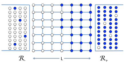
We consider the system in the low temperature region $\beta>\beta_{c}$ and let the spins evolve following a continuos-time stochastic dynamics with two contributions: a conservative exchange dynamics in the bulk and independent spin flips at the boundaries. The dynamics at the boundaries simulates two infinite reservoirs, $\mathscr{R}_{+}$ on the right and $\mathscr{R}_{-}$ on the left, that force a magnetization $m_{+}\in[0,1]$ on the right column and a magnetization $m_{-}=-m_{+}$ on the left column. See Fig. 1 for a description of the set-up in numerical experiments.

Figure 1: Schematic picture of the 2D Ising model coupled to reservoirs $\mathscr{R}_{+}$ and $\mathscr{R}_{-}$. A spins up is represented with a filled (blue) circle, a spin down is represented with an empty (white) circle.

More precisely, in the bulk the spins follow a Kawasaki dynamics, i.e. the spins of a bond $\langle i,j\rangle$ exchange values at rate

$$c(i,j)=\left\{\begin{array}[]{ll}1&\text{if }\Delta H=H(\sigma^{ij})-H(\sigma)\leq 0\\ e^{-\beta\Delta H}&\text{otherwise}\end{array}\right.$$

where $\sigma^{ij}$ denotes the configuration obtained from $\sigma$ by exchanging the spins at sites $i$ and $j$. At the horizontal boundaries the spins flip independently, i.e. they change sign at rate

$$c_{-}(i)=\frac{1-\sigma_{i}m_{-}}{2}\qquad\text{if}\quad i=(1,y)$$

$$c_{+}(i)=\frac{1-\sigma_{i}m_{+}}{2}\qquad\text{if}\quad i=(L,y)$$

Due to the presence of the reservoirs the dynamics is not reversible w.r.t. the Boltzmann-Gibbs measure with Hamiltonian (1). A non-equilibrium steady state sets in characterized by a uniform current in the horizontal direction. A similar setting has been considered in spohn , where the stable region with normal mass transport was considered and the fluctuations of the interface separating the two phases were studied. Thus, the focus in spohn was different than in our paper.

As a result of the simulations we observe the following phenomenology: as $m_{+}$ decreases from $m_{+}=1$ the current is first negative and, past a critical value $m_{crit}$, it becomes positive. We conclude from the simulations that:

• If $m_{+}>m_{crit}$ then the magnetization flows from the plus to the minus phase (from $\mathscr{R}_{+}$ to $\mathscr{R}_{-}$) so that the current is negative (in agreement with the Fick’s law) and the current goes downhill.

• If $m_{+}<m_{crit}$ the magnetization flows from the minus to the plus phases (from $\mathscr{R}_{-}$ to $\mathscr{R}_{+}$), thus the current is positive and we have “uphill diffusion”.

As we shall see, the value of the critical magnetization marking the transition from down- to up-hill diffusion $m_{crit}=m_{crit}(\beta,L)$ is a function of both the inverse temperature $\beta$ and the system size $L$. For simplicity, we avoid in the following to write explicitly such dependences. Our results suggest that in the limit of large boxes $L\to\infty$ the critical magnetization approaches the equilibrium spontaneous magnetization $m_{\beta}$.

Numerical analysis of the current. The integrated current $J_{t}$ over any horizontal bond up to time $t$ can be measured by counting the number of positive spins that cross the bond from left to right minus the number of positive spins that cross the bond in the opposite direction. The current $J$ in the stationary state is then obtained as $J=\lim_{t\to\infty}J_{t}/t$. We have fixed $\beta=1$ and run computer simulations with $L\leq 40$ for various values of $m_{+}$ and $m_{-}=-m_{+}$. We imposed periodic b.c. on the direction orthogonal to the current. Namely, denoting by $i=(x,y)$ the coordinates of site $i$, we set $\sigma_{(x,L+1)}=\sigma_{(x,1)}$ for all $x=1,\ldots,L$. On the longitudinal direction we considered two types of boundary conditions: (a) fixed b.c., i.e. $\sigma_{(0,y)}=-1$, $\sigma_{(L+1,y)}=+1$ for all $y=1,\ldots,L$; (b) shifted b.c., namely we let $\sigma_{(1,y)}$ interact with $\sigma_{(1,y-L/4)}$ and $\sigma_{(L,y)}$ interact with $\sigma_{(L,y-L/4)}$. We will explain later this choice of b.c. (that is inspired by bodineaupresutti ). No difference in the results obtained using the two different boundary conditions on the longitudinal direction was observed in our simulations.

We run two independent programs by implementing both the classical Metropolis Monte Carlo method as well as the kinetic Monte Carlo method kratzer . Whereas the two dynamics yield the the same stationary state, the first algorithm is better suited to measure the current and the second, which implements a continuous time dynamics, is more efficient to probe the magnetization time average.

Our main result is illustrated in Fig. 2. There it is plotted the current $J$ as a function of the right reservoir magnetization $m_{+}$, which varies in the interval $[0.9975,1]$ in steps of $10^{-4}$. The current has to be measured over a sufficiently long time span to get rid of fluctuations and to ensure the convergence to the stationary regime. This can be tested by monitoring the running average of the current and looking at the scale of its fluctuations. As a result, we have verified that $10^{12}$ spin exchanges are needed to guarantee fluctuations of order $10^{-7}$ in the worst cases. In Fig. 2 errors bars are smaller than the size of the points. From Fig. 2 we see the existence of a critical value $m_{crit}\approx 0.99931$ such that if $m_{+}>m_{crit}$ then the current is negative, and if $m_{+}<m_{crit}$ the current is positive. To let better appreciate the change of sign we plot in the inset the integrated current $J_{t}$ up to time $t=3\times 10^{8}$ steps. We see that for $m_{+}=0.99950$ there is a straight line with a negative slope, whereas for $m+=0.99910$ we measure a positive slope.

Figure 2: Current vs. reservoir magnetization for system size $L=40$. Each data point is the current $J$ measured in the non-equilibrium stationary state with a given value $m_{+}$ on the right reservoir $\mathscr{R}_{+}$ and $m_{-}=-m_{+}$ on the left reservoir $\mathscr{R}_{-}$. The inset shows the integrated current $J_{t}$ up to time $t=3\times 10^{8}$ steps for $m_{+}=0.9995$ (negative slope) and for $m+=0.99910$ (positive slope). The initial datum used in the Monte Carlo simulations is: $\sigma_{(x,y)}=-1$ for $x\in[1,L/2]$ and $\sigma_{(x,y)}=1$ for $x\in(L/2,L]$.

In order to gain some understanding on the transition from down- to up-hill diffusion we start from equilibrium (i.e. the setting without reservoirs) considering the canonical Gibbs measure with Hamiltonian (1), inverse temperature $\beta>\beta_{c}$ and total magnetization $m=0$. This is the Wulff problem first studied in dks . For a system of large linear size $L$ it is proved in dks that the typical configurations have the following structure: there is a vertical strip centered at $L/2$ of macroscopically infinitesimal thickness: to the right of the strip the magnetization is essentially $m_{\beta}$ and to the left $-m_{\beta}$ (or viceversa).

In the non-equilibrium setting the interface separating the plus and minus phase is perturbed by the current originated by the reservoirs, while the optimal magnetization profile must also interpolate between the value at the right side $m_{+}$ and its negative value $m_{-}=-m_{+}$ at the left side. When $m_{+}=1$ one expects that the instanton is stable: the magnetization profile $m(r)$ in the macroscopic coordinate $r=x/L$ (thus $r\in[0,1]$) starts from $m(0)=-1$, for $r<1/2$ increases monotonically to $-m_{\beta}$, at $r=1/2$ it has a jump of magnitude $2m_{\beta}$ and finally increases monotonically again for $r>1/2$ from $m_{\beta}$ to $m(1)=1$. Such profile sustains a negative current, which is microscopically due to positive spins (resp. negative) that cross the interface from the right (resp. left) and are eventually absorbed by the left (resp. right) reservoir.

When $m_{+}<1$ a second microscopic mechanism produces a current: positive spins (resp. negative) that are created at the left (resp. right) reservoir and travel to the right (resp. left), thus yielding a positive contribution to the current. Indeed, we see in Fig. 2 that the current increases as $m_{+}$ is decreased from $1$. At $m_{+}=m_{crit}$ the two contributions to the current of microscopic origin balance themselves, thus yielding zero current. Past $m_{crit}$ the positive contribution to the current is dominant.

Figure 3: Spin configurations (top panels) and time-averaged magnetization profiles (bottom panels) for three values of the reservoir magnetization: $m_{+}=-m_{-}=0.9995$ stable phase (first column); $m_{+}=-m_{-}=0.9990$ meta-stable phase (second column); $m_{+}=-m_{-}=0.9980$ weakly-unstable phase (third column).

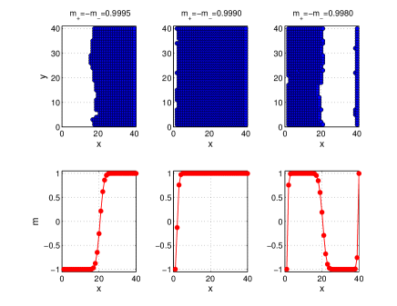
The analysis of the typical spin configurations and time-averaged magnetization profiles show that past $m_{crit}$ there is a change in the structure of the non-equilibrium steady state. We run a simulation with kinetic Monte Carlo method doing $10^{10}$ spin exchanges and plot in Fig. 3 the spin configuration at the end of the run (top panels) and the time averaged magnetization profiles (bottom panels). Whereas for $m_{+}>m_{crit}$ the non-equilibrium stationary state is still concentrated on the instanton profile (Fig. 3, first column), for $m_{+}<m_{crit}$ we see from the numerical simulations that the instanton becomes unstable. Two regimes can be clearly detected: a metastable phase where the instanton is replaced by a bump (Fig. 3, second column) and, continuing to lowering $m_{+}$, a weakly-unstable phase appears with a profile with two bumps (Fig. 3, third column). Note that in Fig. 2 the current has a discontinuity around $m_{+}\simeq 0.9987$, which signals the onset of a dynamical transition from the “bump“ typical configuration (in the metastable region) to the “two-bumps“ configuration (in the weakly-unstable region). Remarkably, a similar scenario was also observed in (CDMPjsp2017, , Fig. 14) in the case of a 1D particle system equipped with an attractive long-range Kac potential.

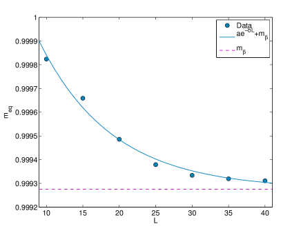
Estimate of the critical magnetization. We claim that the critical value $m_{crit}$ of $m_{+}$ can be estimated with an independent method. Following the theory given in bodineaupresutti , the key quantity is the magnetization value $m_{eq}$ on the rightmost column of the lattice measured at equilibrium, i.e. in the absence of reservoirs. We claim that $m_{eq}$ must be very close to $m_{crit}$. Indeed if $m_{+}=m_{eq}$ (and $m_{-}=-m_{eq}$) then in the non-equilibrium setting the reservoirs are trying to impose a magnetization which is already there, so that their influence is negligible. Therefore the current in the presence of the reservoirs is essentially the current without reservoirs, which is zero. The choice of the shifted b.c. guarantees that even close to the boundaries one would see in a very large system a magnetization $m_{\beta}$ to the right of the interface and $-m_{\beta}$ to the left. However when $L$ is finite the magnetization at the boundaries is not exactly equal to $m_{\beta}$ due to finite-size effects. Thus $m_{eq}$ at finite volume might well be different from $m_{\beta}$. For a system size $L=40$ the simulation at equilibrium yields a value for $m_{eq}\approx 0.99931$, thus in perfect agreement with the value of $m_{crit}$ obtained from the non-equilibrium simulations. We measured the value of $m_{eq}$ for several system sizes with $L$ in the range $[10,40]$. We found that these values decrease with increasing $L$. A plot against $L$ is shown in Fig 4, together with an exponential fit. The extrapolation to the infinite volume is compatible with an asymptotic value of $m_{eq}$ equal to $0.99927$, that coincides approximatively with $m_{\beta}$ in (2) evaluated at $\beta=1$.

Figure 4: Time-averaged magnetization on the last column $m_{eq}$ at equilibrium (i.e. without reservoirs) versus system size $L$. The horizontal line is $m_{\beta}\approx 0.99927$. The continuous line is an exponential fit $m_{\beta}+ae^{-bL}$ with $a=0.00153$ and $b=0.0996$.

Discussion. In this paper it is argued that uphill diffusion appears in the non-equilibrium Ising model coupled to magnetization reservoirs. A few final comments are in order. First we observe that our results imply no violation of the thermodynamic principles. Indeed, our system (composed of a channel and left/right reservoirs) is not an isolated system. On the contrary, the Glauber dynamics at the boundaries is such that energy is systematically pumped into the channel. A second issue is the extrapolation to the thermodynamic limit $L\to\infty$. While this remains an admittedly open issue, we observe that our simulations with $L=40$ provides perfect agreement between the critical magnetization value $m_{crit}$ signaling the onset of uphill diffusion and the magnetization value $m_{eq}$ measured at equilibrium on the rightmost column of the lattice. Furthermore, in the range $L\in[10,40]$ we could verify the expected exponential convergence of $m_{eq}$ to equilibrium spontaneous magnetization $m_{\beta}$. All this is evidence that our non-equilibrium simulations are capable of reproducing the infinite volume equilibrium state including its finite volume corrections. We are currently investing larger sizes future to verify the conjecture that uphill diffusion persists in the thermodynamical limit $L\to\infty$.

The apparent contradiction between uphill diffusion and the validity of Fick’s law can be resolved by looking at the magnetization profiles. Specifically, in the second column of Fig. 3 we measured a value of magnetization at the peak of the bump that is between $m_{+}$ and $m_{\beta}$, namely $m_{+}=0.9990<m_{bump}=0.99925<m_{\beta}\approx 0.99927$. In between the peak and the right boundary, the magnetization profile is monotonically decreasing, thus most of the magnetization profile is compatible with a positive current that is down the gradient. In the third column of Fig. 3 we found instead $m_{+}=0.9980<m_{\beta}\approx 0.99927<m_{bump}=0.99940$. Thus, being $m_{\beta}<m_{bump}$, we have again downhill current.

It is natural to ask what is the structure of the non-equilibrium stationary state as one continues to lower $m_{+}$. We see from the simulations that the weakly-unstable region with a double bump persists until, approximately, the value $m_{+}=0.92$. We do not investigate here what happens below this value, where one enters a chaotic region with the stationary measure dominated by several typical configurations. We will report results on the chaotic region elsewhere.

Acknowledgements. The authors wish to thank A. De Masi and E. Presutti who inspired this work and supported our research with illuminating discussions. M.C. acknowledges useful discussions with M. Kröger on the implementation of Monte Carlo simulations. We acknowledge financial supports from Fondo di Ateneo per la Ricerca 2015 and 2016 (UniMoRe). Part of this work was done during the authors stay at the Institute Henri Poincaré during the trimester “Stochastic Dynamics Out of Equilibrium”.

References

- (1) J. Fourier, Théorie analytique de la chaleur, Chez Firmin Didot, père et fils (1822).
- (2) L.S. Darken, Trans. Aime 180, 430 (1949).
- (3) R. Krishna, Chem. Soc. Rev. 44, 2812 (2015).
- (4) C. Bernardin, S. Olla, J. Stat. Phys. 145, 1224 (2011).
- (5) A. Iacobucci, F. Legoll, S. Olla, G. Stoltz, Phys. Rev. E 84, 061108 (2011).
- (6) R. Krishna, Phys. Chem. Chem. Phys. 17, 27428 (2015).
- (7) R. Krishna, Ind. Eng. Chem. Res. 55, 1053 (2016).
- (8) R. Krishna, Curr. Opin. Chem. Eng. 12, 106 (2016).
- (9) A. De Masi, E. Presutti, D. Tsagkarogiannis, Arch. Rat. Mech. 201, 681(2011).
- (10) M. Colangeli, A. De Masi, E. Presutti, Phys. Lett. A 380, 1710 (2016).
- (11) M. Colangeli, A. De Masi, E. Presutti, J. Stat. Phys. 167, 1081 (2017).
- (12) M. Colangeli, A. De Masi, E. Presutti, J. Phys. A: Math. Theor. 50 435002 (2017).
- (13) H. Spohn, Z. Phys. B 97, 361 (1995).
- (14) L. Onsager, Phys. Rev. 65, 117 (1944).
- (15) C. N. Yang, Phys. Rev. 85, 808 (1952).
- (16) T. Bodineau, E. Presutti, Ann. Henri Poinc., 4, 847 (2003).
- (17) P. Kratzer, Multiscale Sim. Meth. Molecular Sc., 42, 51 (2009).
- (18) R. Dobrushin, R. Kotecký, S. Shlosman, Wulff construction: a global shape from local interaction, Vol. 104, Providence, Rhode Island: American Mathematical Society, (1992).
- (19) M. Colangeli, C. Giardinà, C. Giberti, M. Kröger, C. Vernia, in preparation.