Hollowness in $pp$ scattering at the LHC

Abstract

We examine how the effect of hollowness in $pp$ scattering at the LHC (minimum of the inelasticity profile at zero impact parameter) depends on modeling of the phase of the elastic scattering amplitude as a function of the momentum transfer. We study the cases of the constant phase, the Bailly, and the so called standard parameterizations. It is found that the 2D hollowness holds in the first two cases, whereas the 3D hollowness is a robust effect, holding for all explored cases.

In this contribution we focus on the aspects of the alleged hollowness effect in $pp$ scattering not covered in our previous paper [1] and talks [2, 3], where the basic concepts and further details of the presented analysis may be found. The recent TOTEM [4] and ATLAS (ALFA) [5] data for the differential elastic cross section for $pp$ collisions at $\sqrt{s}=7$ TeV and $\sqrt{s}=8$ TeV [6, 7] suggest a stunning behavior (impossible to explain on classical grounds), where more inelasticity in the reaction occurs when the protons collide at an impact parameter $b$ of a fraction of a fermi, than for head-on collisions. Here we discuss the sensitivity of this hollowness feature on modeling of the phase of the elastic scattering amplitude as a function of the momentum transfer. In previous analyses [1, 8, 9, 10, 11, 12, 13, 14, 15, 16, 17, 18, 19] this effect was not treated with sufficient attention.

In the present work we parametrize separately the absolute value and the phase of the strong elastic $pp$ scattering amplitude. For the absolute value we apply the form of Ref. [20]:

$$|{f}(s,t)|=p\left|\frac{i\sqrt{A}e^{\frac{Bt}{2}}}{\left(1-\frac{t}{t_{0}}\right)^{4}}+i\sqrt{C}e^{\frac{Dt}{2}+i\phi}\right|\,,$$ (1)

where $p$ is the CM momentum, and $A$, $B$, $C$, $D$, and $t_{0}$ were adjusted to the data. We neglect spin effects, hence the amplitude is to be understood as spin-averaged. The quality of the fit to differential elastic cross section from the LHC data at $\sqrt{s}=7$ TeV can be assessed from Fig. 1(a). This fit is sensitive only to the square of the absolute value of the amplitude, and not to its phase. However, this is not true of other features of $pp$ scattering, which do depend of the phase.

The $\rho(s,t)$ function is defined as the ratio of the real to imaginary parts of ${f}(s,t)$:

$$\rho(s,t)=\frac{{\rm Re}{f}(s,t)}{{\rm Im}{f}(s,t)},\;\;\;\;\;\;\;{f}(s,t)=\frac{i+\rho(s,t)}{\sqrt{1+\rho(s,t)^{2}}}|{f}(s,t)|.$$ (2)

At $t=0$, $\rho(s,0)$ can be determined when the total cross section $\sigma_{\rm tot}(s)$ and the differential cross section extrapolated to $t=0$ are know. In actual analyses, interference with the Coulomb amplitude is used to determine $\rho$ (see in particular Ref. [21] for further information and literature). The value of the phase at $t=0$ for $\sqrt{s}=7$ TeV has been determined to be $\rho(7~{}{\rm TeV},0)=0.145(100)$ [4]. However, one should bear in mind that the extraction of the dependence of $\rho(s,t)$ on $t$ via the separation of the electromagnetic and strong amplitudes [22] is sensitive to the internal electromagnetic structure of the proton and is subject to on-going debate [23].

In this contribution we explore three popular parameterizations: constant,

$$\rho(t)=\rho_{0}={\rm const.},$$ (3)

with $\rho_{0}=0.14$, the Bailly et al. [24] parametrization,

$$\rho(t)=\frac{\rho_{0}(s)}{1-t/t_{d}},$$ (4)

where $t_{d}=0.52~{}{\rm GeV}^{2}$ is the position of the diffractive minimum, and the so called standard parametrization

$$\rho(t)=\rho_{0}+\frac{\left(\rho_{0}^{2}+1\right)\tau t}{\tau^{2}+t_{0}^{2}-\left(\rho_{0}\tau+t_{0}\right)t}$$ (5)

with $t_{0}=0.5~{}{\rm GeV}^{2}$ and $\tau=0.1~{}{\rm GeV}^{2}$.

The $b$ representation the scattering amplitude is defined via the Fourier-Bessel transform of $f(s,t)$, as given by the data parametrization,

$$2ph(b,s)=2\int_{0}^{\infty}qdqJ_{0}(bq)f(s,-q^{2})={i}\left[1-e^{i\chi(b)}\right],$$

where we have also introduced the eikonal phase $\chi(b)$.

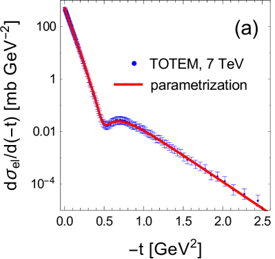
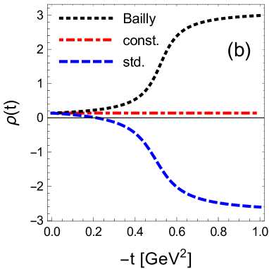
Figure 1: (a) Data for the differential elastic strong-interaction cross section at the LHC energy of $\sqrt{s}=7$ TeV [4] with the overlaid fit of Eq. 1. (b) Phase of the strong-interaction elastic scattering amplitude, according to the three models of Eq.(3-5).

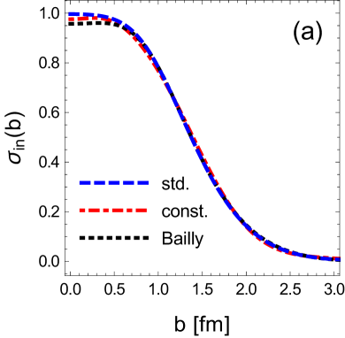
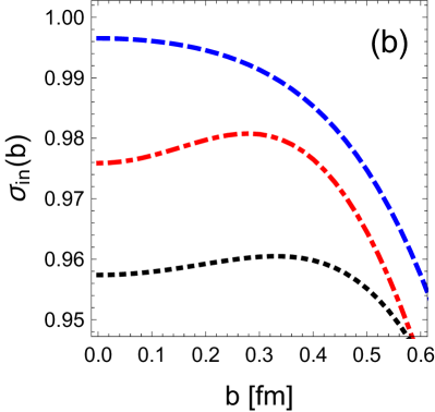
Figure 2: (a) Inelastic cross section in the impact-parameter representation for three models of $\rho(t)$ from Eq.(3-5). (b) Close-up for small values of $b$.

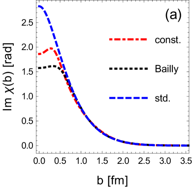
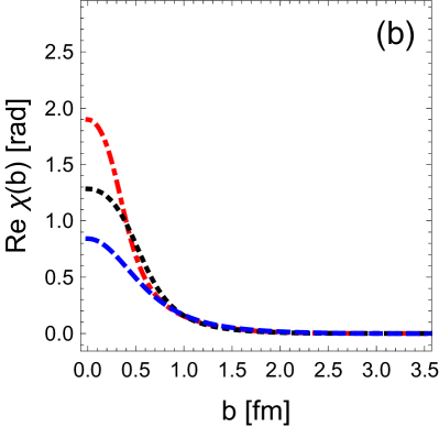
Figure 3: Same as in Fig. 2, but for the imaginary (a) and real (b) parts of the eikonal scattering phase.

The equation for the inelastic cross section is

$$\sigma_{\rm in} \equiv \sigma_{T}-\sigma_{\rm el}=\int d^{2}b\left(4p{\rm Im}h(b,s)-4p^{2}|h(b,s)|^{2}\right),$$ (6)

where the integrand is the inelasticity profile, with $0\leq\sigma_{\rm in}(b)\leq 1$.

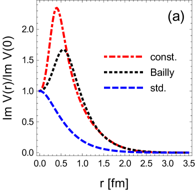
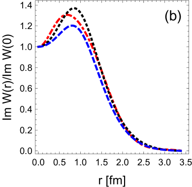
Figure 4: Imaginary parts of the optical potential $V(r)$ (a) and the on-shell optical potential $W(r)$ (b), introduced in Refs. [2, 1], plotted for parameterizations of $\rho(t)$ from Eq.(3-5).

In Fig. 2 we show $\sigma_{\rm tot}(b)$ for three parameterizations $\rho(t)$ of Eq.(3-5). We note that hollowness appears for the first two models, whereas it is absent for the “standard” parametrization. The imaginary and real parts of the eikonal phase are presented in Fig. 3, where we note the corresponding dips at $b=0$ for the imaginary parts – a feature that follows from the eikonal formalism [3].

Finally, in Fig. 4 we show the imaginary parts of the optical potential $V(r)$ and the on-shell optical potential $W(r)$, introduced in Refs. [2, 1]. We note that in this 3D picture of $pp$ scattering, hollowness occurs for all the considered models of $\rho(t)$.

To summarize, a firm establishment of the 2D hollowness requires a careful determination of the phase of the strong-interaction elastic amplitude. On the other hand, hollowness in 3D is a robust effect. The intriguing property of hollowness must have quantum origin [2, 3], hence touches upon very basic features of the scattering mechanism. Hopefully, future data and more refined analyses based on the Coulomb separation will sort out the issue in 2D.

References

- Ruiz Arriola and Broniowski [2017] E. Ruiz Arriola and W. Broniowski, Phys. Rev. D95, 074030 (2017), arXiv:1609.05597 [nucl-th] .
- Ruiz Arriola and Broniowski [2016] E. Ruiz Arriola and W. Broniowski, Proceedings, Theory and Experiment for Hadrons on the Light-Front (Light Cone 2015): Frascati, Italy, September 21-25, 2015, Few Body Syst. 57, 485 (2016), arXiv:1602.00288 [hep-ph] .
- Broniowski and Ruiz Arriola [2017] W. Broniowski and E. Ruiz Arriola, Proceedings, 23rd Cracow Epiphany Conference on Particle Theory Meets the First Data from LHC Run 2: Cracow, Poland, January 9-12, 2017, Acta Phys. Polon. B48, 927 (2017), arXiv:1704.03271 [hep-ph] .
- Antchev et al. [2013a] G. Antchev et al. (TOTEM), Europhys. Lett. 101, 21002 (2013a).
- Aad et al. [2014] G. Aad et al. (ATLAS), Nucl. Phys. B889, 486 (2014), arXiv:1408.5778 [hep-ex] .
- Antchev et al. [2013b] G. Antchev et al. (TOTEM), Phys. Rev. Lett. 111, 012001 (2013b).
- Aaboud et al. [2016] M. Aaboud et al. (ATLAS), Phys. Lett. B761, 158 (2016), arXiv:1607.06605 [hep-ex] .
- Alkin et al. [2014] A. Alkin, E. Martynov, O. Kovalenko, and S. M. Troshin, Phys. Rev. D89, 091501 (2014), arXiv:1403.8036 [hep-ph] .
- Dremin [2015a] I. M. Dremin, Bull. Lebedev Phys. Inst. 42, 21 (2015a), [Kratk. Soobshch. Fiz.42,no.1,8(2015)], arXiv:1404.4142 [hep-ph] .
- Dremin [2015b] I. M. Dremin, Phys. Usp. 58, 61 (2015b), arXiv:1406.2153 [hep-ph] .
- Dremin [2017a] I. M. Dremin, Phys. Usp. 60, 333 (2017a), arXiv:1610.07937 [hep-ph] .
- Dremin [2017b] I. M. Dremin, (2017b), arXiv:1702.06304 [hep-ph] .
- Dremin [2017c] I. M. Dremin, Usp. Fiz. Nauk 187, 353 (2017c).
- Anisovich et al. [2014] V. V. Anisovich, V. A. Nikonov, and J. Nyiri, Phys. Rev. D90, 074005 (2014), arXiv:1408.0692 [hep-ph] .
- Albacete and Soto-Ontoso [2017] J. L. Albacete and A. Soto-Ontoso, Phys. Lett. B770, 149 (2017), arXiv:1605.09176 [hep-ph] .
- Troshin and Tyurin [2017a] S. M. Troshin and N. E. Tyurin, J. Phys. G44, 015003 (2017a), arXiv:1603.07111 [hep-ph] .
- Troshin and Tyurin [2016] S. M. Troshin and N. E. Tyurin, Mod. Phys. Lett. A31, 1650079 (2016), arXiv:1602.08972 [hep-ph] .
- Troshin and Tyurin [2017b] S. M. Troshin and N. E. Tyurin, Eur. Phys. J. A53, 57 (2017b), arXiv:1701.01815 [hep-ph] .
- Troshin and Tyurin [2017c] S. M. Troshin and N. E. Tyurin, Int. J. Mod. Phys. A32, 1750103 (2017c), arXiv:1704.00443 [hep-ph] .
- Fagundes et al. [2013] D. A. Fagundes, A. Grau, S. Pacetti, G. Pancheri, and Y. N. Srivastava, Phys.Rev. D88, 094019 (2013), arXiv:1306.0452 [hep-ph] .
- Antchev et al. [2016] G. Antchev et al. (TOTEM), Eur. Phys. J. C76, 661 (2016), arXiv:1610.00603 [nucl-ex] .
- West and Yennie [1968] G. B. West and D. R. Yennie, Phys. Rev. 172, 1413 (1968).
- Prochazka and Kundrat [2016] J. Prochazka and V. Kundrat, (2016), arXiv:1606.09479 [hep-th] .
- Bailly et al. [1987] J. L. Bailly et al. (EHS-RCBC), Z. Phys. C37, 7 (1987).
- Godizov [2017] A. A. Godizov, (2017), arXiv:1705.09126 [hep-ph] .