Exponentially Twisted Sampling: a Unified Approach for Centrality Analysis in Attributed Networks
Abstract
In our recent works, we developed a probabilistic framework for structural analysis in undirected networks and directed networks. The key idea of that framework is to sample a network by a symmetric and asymmetric bivariate distribution and then use that bivariate distribution to formerly defining various notions, including centrality, relative centrality, community, and modularity. The main objective of this paper is to extend the probabilistic definition to attributed networks, where sampling bivariate distributions by exponentially twisted sampling. Our main finding is that we find a way to deal with the sampling of the attributed network including signed network. By using the sampling method, we define the various centralities in attributed networks. The influence centralities and trust centralities correctly show that how to identify centralities in signed network. The advertisement-specific influence centralities also perfectly define centralities when the attributed networks that have node attribute. Experimental results on real-world dataset demonstrate the different centralities with changing the temperature. Further experiments are conducted to gain a deeper understanding of the importance of the temperature.
Index Terms:
centralities, signed networks, sampled graph, exponentially twisted sampling.I Introduction
In social network analysis, centrality [1, 2, 3] have been widely used for ranking the important nodes. To obtain a viewpoint of a network, one typical method is to ”sample” the network, e.g., edge sampling, random walks, diffusion [4], or random gossiping [5]. Mathematically, each sampling method renders a (probability) measure for a network that enables us to carry out further analysis. As in the probabilistic framework in [6], we model a network as a graph and “sample” the graph to generate a bivariate distribution for a pair of two nodes. In this paper, we only consider the case that the bivariate distribution is symmetric. Under this assumption, the two marginal distributions of the bivariate distribution are the same. As such, the marginal distribution can be used for defining the centrality. Then, we can use centrality to rank nodes. Ranking nodes in the unsigned network have existed a long time such as PageRank [7]. There are many papers in the development of new centralities has made great progress in a static network [8, 9, 10]. Moreover, they extend network properties to the dynamic network [11, 12]. Also, many researchers have proposed heuristics on the standard methods to make them computable in signed networks [13] and attributed network [14], but there is no unified approach for centrality. In this paper, we propose ”exponentially twisted sampling,” the exponential change of measure to get the bivariate distribution , to sample the graph . We show that our centrality measure digs out various centrality, including the influence centralities, the trust centralities, the advertisement-specific influence centralities, and homophily centrality.
The main objective of this paper is to extend the centrality in [6, 15, 16] to attributed networks which contain edge attribute and node attribute. Our main finding is that we can find the path measure to sample the path . For this, we show that one can construct another sampled graph with a exponentially twisted sampling, and then the path measure can be represented as a function of attributes of the nodes and edges along the path. In this paper, we also address a method for sampling an attributed network with a bivariate distribution and a path measure.
II Sampled graph
II-A Review of the probabilistic framework of sampled graphs
In [15, 16], a probabilistic framework for structural analysis in undirected/directed networks was proposed. The main idea in that framework is to sample a network by randomly selecting a path in the network. A network with a path sampling distribution is then called a sampled graph in [15, 16] that can in turn be used for structural analysis of the network, including centrality and community. Specifically, suppose a network is modeled by a graph , where denotes the set of vertices (nodes) in the graph and denotes the set of edges (links) in the graph. Let be the number of vertices in the graph and index the vertices from . Also, let be the adjacency matrix of the graph, i.e.,
| (3) |
Let be the set of (directed) paths from to and be the set of paths in the graph . According to a probability mass function , called the path sampling distribution, a path is selected at random with probability . In [15, 16], there are many methods for sampling a graph with a randomly selected path. Here we introduce the following three commonly used approaches: (i) sampling by uniformly selecting a directed edge, (ii) sampling by a Markov chain, and (iii) sampling by a random walk on an undirected network with path length 1 or 2.
Example 1.
(Sampling by uniformly selecting a directed edge) Given a directed graph with the adjacency matrix , one only sample directed paths with length 1 and this is done uniformly among all the directed edges. Specifically, sampling by uniformly selecting a directed edge has the following probability mass function:
| (6) |
where is the total number of directed edges in the graph.
Example 2.
(Sampling by a Markov chain) Given a directed graph with the adjacency matrix , consider an ergodic Markov chain on this graph. Let be the transition probability from node to node and be the steady state probability of node . In particular, for PageRank [17] with the web surfing probability , the transition probability of the corresponding Markov chain is
| (7) |
where is the out-degree of node . Its steady state probabilities (with ) can be obtained from solving the following system of equations:
| (8) |
For a path that traverses a sequence of nodes in a directed network, we have from the Makrov property that
| (9) |
Consider the reverse path of , denoted by , that traverses a sequence of nodes . If the Markov chain is reversible, then it follows from the detailed balance equation that
| (10) |
It is known that the corresponding Markov chain for PageRank is in general not reversible. However, the corresponding Markov chain for a random walk on an undirected graph is reversible. We will discuss this further in the next example.
Example 3.
(Sampling by a random walk on an undirected network with path length 1 or 2) For an undirected graph , let be the total number of edges and be the degree of node , . A path with length 1 can be represented by the two nodes it traverses. Similarly, a path with length 2 can be represented by the three nodes it traverses. A random walk with path length not greater than 2 can be generated by the following two steps: (i) with the probability , an initial node is chosen, (ii) with probability , , a walk with length is chosen. As such, we have
| (14) |
where and , . For an undirected network, we have for all . Thus, in view of (14), we also have
| (15) |
in this example.
Let (resp. ) be the starting (resp. ending) node of a randomly select path by using the path sampling distribution . Then the bivariate distribution
| (16) |
is the probability that the ordered pair of two nodes is selected. As such, can be viewed as a similarity measure from node to node and this leads to the definition of a sampled graph in [15, 16]. In general, the bivariate distribution in (16) is not symmetric by using the path sampling distributions in Example 1 and Example 2. However, if for any path , then the bivariate distribution in (16) is clearly symmetric.
Definition 4.
Let (resp. ) be the marginal distribution of the random variable (resp. ), i.e.,
| (17) |
and
| (18) |
Then is the probability that node is selected as a starting node of a path and it can be viewed as an out-centrality of . On the other hand, is the probability that node is selected as a ending node of a path and it can be viewed as an in-centrality of . The in-centrality and the out-centrality are in general not the same. Clearly, if the bivariate distribution is symmetric, then the in-centrality and the out-centrality are the same. A recent advance in [16] shows that one does not need a symmetric bivariate distribution to ensure the equality between the in-centrality and the out-centrality. In particular, for the Markov chain sampling methods in Example 2, one still has and the in-centrality and the out-centrality are the same. In that case, we will simply refer as the centrality of node .
The framework of sampled graphs in [15, 16] can further be used to define the notions of community and modularity. There are two different types of communities for directed networks that are commonly addressed in the literature (see e.g., [18, 19]): structural communities (based on the densities of edges) and flow communities (based on the flow of probabilities). For (probabilistic) flow communities, they can be detected by using Markov chains in Example 2. On the other hand, structural communities can be detected by using uniform edge sampling in Example 1 to produce communities that are densely connected inside and sparsely connected outside. These two notions of community and modularity will not be pursued further in this paper.
II-B Exponentially twisted sampling
Now we generalize the probabilistic framework in [15, 16] to attributed networks. An attributed network is a generalization of a graph by assigning each node an attribute and each edge an attribute . As such, an attributed network can be represented as , where and are called the node attribute function and the edge attribute function, respectively.
For a path that traverses a sequence of nodes in a attributed network, we can define a path measure as a function of the attributes of the nodes and edges along the path , i.e.,
In this paper, we assume that a path measure is a mapping from the set of paths to a -dimensional real-valued vector in , i.e.,
where , , are real-valued functions.
Now suppose that we have already had a sampled graph that uses the probability mass function to sample a path in . The question is how the sampling distribution should be changed so that the average path measure is equal to a specified vector . In other words, what is the most likely sampling distribution that leads to the average path measure given that the original sampling distribution is ? For this, we introduce the Kullback-Leibler distance between two probability mass functions and :
| (19) |
The Kullback-Leibler distance is known to be nonnegative and it is zero if and only if (see e.g., [20]). Also, according to the Sanov theorem (see e.g., the books [20, 21]), the larger the Kullback-Leibler distance is, the more unlikely for to behave like . Thus, to address the question, we consider the following constrained minimization problem:
| (20) | |||||
The first constraint states that the total probability must be equal to . The second constraint states that the average path measure must be equal to with the new sampling distribution . The above minimization problem can be solved by using Lagrange’s multipliers and as follows:
| (21) |
Taking the partial derivative with respect to yields
| (22) |
Thus,
| (23) |
Since , it then follows that
| (24) |
where
| (25) |
is the normalization constant. The new sampling distribution in (24) is known as the exponentially twisted distribution in the literature (see e.g., [22]).
To solve , we let
The quantity is called the free energy as it is analogous to the free energy in statistical mechanic [2]. It is easy to see that for that
| (26) |
These equations can then be used to solve , .
Once we have the sampling distribution in (24), we can define a bivariate distribution as in (16). Specifically, let (resp. ) be the starting (resp. ending) node of a randomly select path according to the sampling distribution in (24). Then the bivariate distribution
| (27) |
is the probability that the ordered pair of two nodes is selected and it can be viewed as a similarity measure from node to node . Analogous to the discussion of a sampled graph in the previous section, the marginal distribution of the random variable (resp. ), i.e., (resp. ), can be viewed as an out-centrality of (resp. in-centrality of ).
III Centralities
III-A Centralities in signed networks
In this section, we consider a special class of attributed networks, called signed networks. A signed network is an attributed network with an edge attribute function that maps every undirected edge in to the two signs . In this paper, we represent the positive (resp. negative) sign by 1 (resp. -1). An edge mapped with the sign is called a positive edge, and it is generally used for indicating the friendship between the two nodes and . On the other hand, an edge mapped with the sign is called a negative edge. A negative edge indicates that and are enemies.
III-A1 Influence centralities
Such a problem was previously studied in [13] for ranking nodes in signed networks. In SRWR [13], a signed random surfer was used. They use the balance theory to imply the signed random walks. In our paper, it is our special case because it is as same as our how to sampling the path. In [13], it divides the equation into positive surfer and negative surfer . However, we can consider positive and negative situations in a comprehensive way.
One interesting question for signed networks is how the nodes in signed networks are ranked. Our idea for this is to use opinion dynamics. If and are connected by a positive (resp. negative) edge, then it is very likely that will have a positive (resp. negative) influence on and vice versa. As such, if we start from a node with a positive opinion on a certain topic, then a neighbor of node connected by a positive (resp. negative) edge will tend to have the same (resp. the opposite) opinion as node has. Now we can let the opinion propagate through the entire network (via a certain opinion dynamic) and count the (expected) number of nodes that have the same opinion as node has. If such a number is large, then it seems reasonable to say that node has a large positive influence on the other nodes in the network. In other words, a node has a large positive influence if there is a high probability that the other end of a randomly selected path has the same opinion as node . This then leads us to define the notion of influence centralities for ranking nodes in signed networks.
The above argument is based on the general belief that “a friend of my friend is likely to be my friend” and “an enemy of my enemy can be my friend” in [2]. As such, for a path that traverses a sequence of nodes in a signed network, we define the following path measure as the product of the edge signs along the path, i.e.,
| (28) |
Note that is either 1 or -1 as the edge attribute function that maps every undirected edge in to . In addition to the path measure, we also need to specify the probability that the path is selected, i.e., in (24). For this, we consider a random walk with path length 1 or 2 in Example 3. It then follows from (24), (28) and (14) that
| (34) |
| (35) |
The constant in (35) is the normalization constant. Summing all the paths from to yields the bivariate distribution
| (36) |
The marginal distribution of the bivariate distribution, denoted by , is the influence centrality of node (with respect to the temperature ).
If we only select paths with length 1, i.e., in (36), then there is a closed-form expression for the influence centrality. For this, we first compute the normalization constant by summing over and in (36) and this yields
| (37) |
where (resp. ) is the total number of positive (resp. negative) edges in the graph. Thus, for ,
| (38) | |||||
where (resp. ) is the number of positive (resp. negative) edges of node .
III-A2 Trust centralities
As discussed in the previous section, the influence centralities are based on the general belief that “an an enemy of my enemy can be my friend.” Such a statement might be valid for modelling opinion dynamics. However, it is not suitable for modelling trust. In addition to the interpretation of a signed edge as the friend/enemy relationship, another commonly used interpretation is the trusted/untrusted link. A path that traverses a sequence of nodes can be trusted if every edge is a trusted link so that there exists a chain of trust. In view of this, we consider another path measure as the minimum of the edge signs along the path, i.e.,
| (41) |
If we use the random walk with path length 1 or 2 to sample a path in as in (14), then the sampling distribution for the signed network with the path measure in (41) can be written as follows:
| (47) |
| (48) |
Moreover, we have the following bivariate distribution
where is the normalization constant. The marginal distribution of the bivariate distribution, denoted by , is the trust centrality of node (with respect to the temperature ). We note that if we only select paths with length 1, i.e., , then the trust centrality is the same as the influence centrality in (38).
III-B Advertisement-specific influence centralities in networks with node attributes
In this section, we consider another class of attributed networks that have node attributes. For a graph with the node attribute function that maps every node to a vector in
| (50) |
One intuitive way to interpret such an attributed network is to view the graph as a social network with users and the attribute vector in (50) as the scores of user on various topics. Now suppose an advertisement can be represented by a vector of scores with being the score of the topic. Then we would like to find out who are the most influential users in the network to pass on the advertisement . Such a problem was previously studied in [14] for ranking nodes in Twitter. In TwitterRank [14], a two-step approach was used. First, a topic-specific ranking is obtained for each topic by using a random surfer model similar to that in PageRank [17]. The second step is then to take the weighted average over these topic-specific rankings. Specifically, suppose that is the ranking for topic and user . TwitterRank for advertisement and user is then defined as the following weighted average:
| (51) |
One flaw for such a two-step approach is that it neglects the fact that the propagation of a specific advertisement through a user depends on how much a user “likes” the advertisement. To model how much a user “likes” an advertisement, we use the similarity measure from the inner product of the score vector of the user and that of the advertisement. It is possible that in a cascade of two users , both users like the advertisement because their inner products are large, but user likes one topic in that advertisement and user likes another different topic in that advertisement. Such a cascade cannot be caught by using the two-step approach in TwitterRank [14]. In view of this, it might be better to use a single-step approach for computing advertisement-specific influence centralities. As the influence centralities in the previous section, we propose using opinion dynamics through a path. For a path that traverses a sequence of nodes in the attributed network, we define the following path measure
| (52) |
where
is the inner product of and , If we use the random walk with path length 1 or 2 to sample a path in as in (14), then the sampling distribution for the attributed network with the path measure in (52) can be written as follows:
| (58) |
| (59) |
Moreover, we have the following bivariate distribution
where is the normalization constant. The marginal distribution of the bivariate distribution, denoted by , is the advertisement-specific influence centrality of node for advertisement (with respect to the temperature ).
IV Experiment
IV-A Experiment for influence centrality
In this section, we evaluate our model on the real-world network proposed in [23] which is a directed network of hyperlinks between weblogs of US politics recorded by Adamic and Glance. The data on political leaning come from blog directories as indicated. Some blogs were labeled manually, based on incoming and outgoing links and posts around the time of the United States presidential election of 2004. Basically, there are 1,490 nodes and 19,090 edges in this dataset. For our purposes, we would like to examine our algorithm in a undirected signed network. Therefore, we choose the nodes from different community and adding 4,000 negative edges to this network. As a reason that every node should be treated fairly, we randomly pick up the node in the different community instead of choosing those with a higher degree. Then let the the adjacency matrix because we want to get the undirected network. Before we rank these nodes, we have to delete the nodes with degree smaller than 7, that is, their ranks are not important. Furthermore, we also remove the edges which are self-loop and the edges between two nodes if they are connected by more than one edges. As a result, we obtain the directed signed network containing 863 nodes and 16,650 edges, including 15,225 positive edges and 1,425 negative edges.
|
|
|
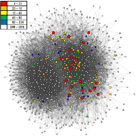
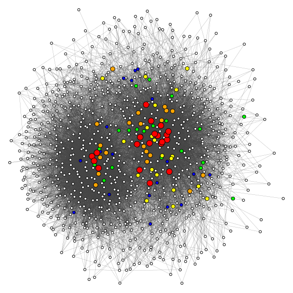
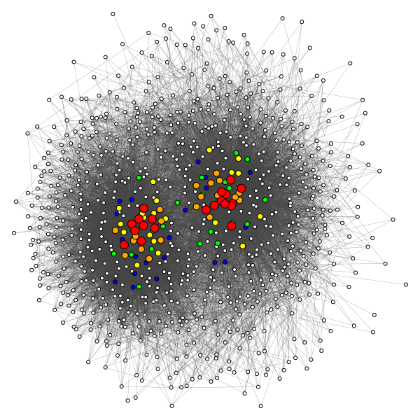
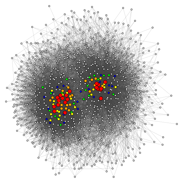
| (a) = -0.9, =-2.6566 | (b) =-0.5, =-1.7337 | (c) =0, =-1.1844 |
|

|
|
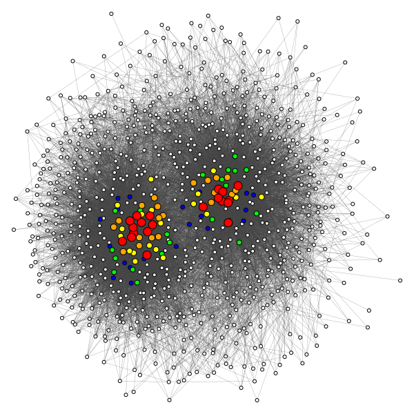
| (d) =0.5, =-0.6351 | (e) =0.9, =0.2878 | (f) =0.99, =1.4623 |
| ranking by positive edge | ranking by negative edge | ranking by total edge | |
|---|---|---|---|
| =-0.99 =-3.8310 | 0.0417 | 0.7544 | 0.0417 |
| =-0.9 =-2.6566 | 0.0753 | 0.6667 | 0.0753 |
| =-0.5 =-1.7337 | 0.2658 | 0.3514 | 0.2658 |
| =0 =-1.1844 | 0.7241 | 0.0989 | 0.7241 |
| =0.5 =-0.6351 | 0.8868 | 0.0638 | 0.8868 |
| =0.9 =0.2878 | 1 | 0.0417 | 0.9608 |
| =0.99 =1.4323 | 1 | 0.0417 | 0.9608 |
IV-A1 Experiment by =0
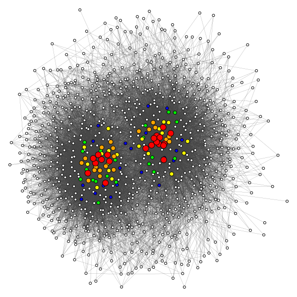
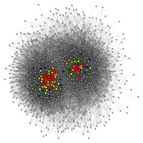
In Figure 1, we show the distribution of ranking by =0. Initially, the top 100 nodes are uniformly distributed on the right side on (a). However, when the value of gamma increases, the top 100 nodes gradually gather in the middle of two community where nodes have more edges than those on the edge of the graph. Also, these top 100 nodes are divided into two clusters and for the nodes in each cluster, they are closely compact with each other. From so, the key persons for these two clusters can be found at ease. On the other hand, we can get the information of which nodes are affecting others in a negative way while gamma is lower. That is to say; these nodes usually have a much higher negative degree compared to others. We can view the nodes with a higher negative degree as people who are sent to attack the opponent team, which we call a hitman in this paper. Since these graphs only provide the fact that the top 100 nodes would gather in the middle of the graph if gamma is close to 1, we use Jaccard index for more detail explanation. The Jaccard index is a statistic used for comparing the similarity and diversity of sample sets. It can be denoted as
| (61) |
where and are the sample sets.
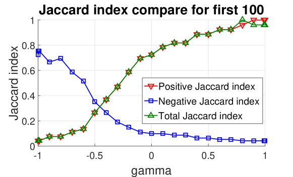
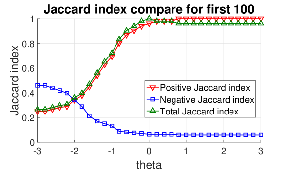
In Table I, we use three kinds of Jaccard index as metrics for comparing the similarity between two sample sets. The negative Jaccard index, the similarity between the set ranked by negative edges and the set ranked by . Similarly, the positive (total) Jaccard index is the similarity between the set ranked by positive (total) edges and the set ranked by . It is easy for us to conclude that the increment of gamma has a positive impact on raising theta. Also, the change of theta causes the change of all three Jaccard indexes. More specifically, the negative Jaccard index decreases and the positive Jaccard index increases along with the increment of theta. Interestingly, the total Jaccard index has a larger value when theta is closer to zero. In order to look into the relationship between these three parameters, Figure 2 is plotted.
|
|
|
| (a) =-3 | (b) =-2 | (c) =-1 |
|

|

|
| (d) =0 | (e) =1 | (f) =2 |
In Figure 2, we can make a conclusion that the positive Jaccard index and the negative Jaccard index have positive and negative relation with gamma respectively. For the total Jaccard index, it has its maximum when gamma is close to 0.8. This implies the fact that the closer to 0.8 the gamma is, the closer to zero the theta is. As a result, we can use this fact as a pioneering method to define the centrality for a signed network. That is to say, the centrality can be defined by the adjustment of temperature (theta). By using opinion dynamic, there are three different centralities able to be defined. First, the positive influence centrality, representing those people who give you positive influences (e.g., your friends), can be found by increasing the temperature (theta). On the contrary, the negative influence centrality stands for those people giving you negative influences like your enemy. We figure it out by lowering down the temperature (theta). Last, the total influence centrality is the representation for the famous people among all. For these famous people, the thing we only care about is how many people know him instead of how many people love him or hate him. Thus, we make the temperature (theta) close to zero to find the total influence centrality.
| ranking by positive edge | ranking by negative edge | ranking by total edge | |
|---|---|---|---|
| =-2 | 0.3423 | 0.3423 | 0.3605 |
| =-1.5 | 0.4925 | 0.1976 | 0.5152 |
| =-1 | 0.6949 | 0.1299 | 0.7241 |
| =-0.5 | 0.8868 | 0.0753 | 0.9231 |
| =0 | 0.9608 | 0.0638 | 1 |
| =0.5 | 0.9802 | 0.0638 | 0.9802 |
| =1 | 1 | 0.0582 | 0.9608 |
| =1.5 | 1 | 0.0582 | 0.9608 |
| =2 | 1 | 0.0582 | 0.9608 |
|

|

|
| (a) =0 | (b) =1 | (c) =2 |
IV-A2 Experiment by and
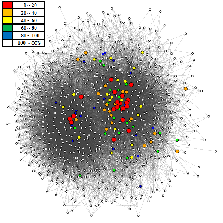
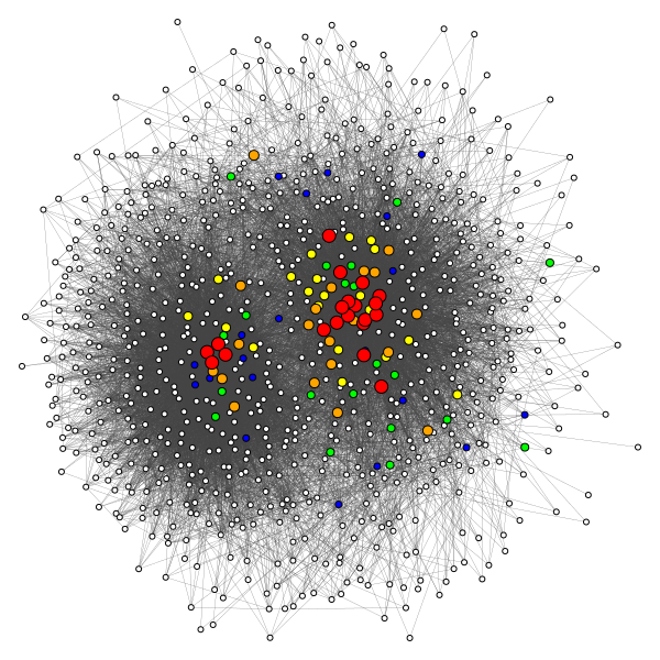
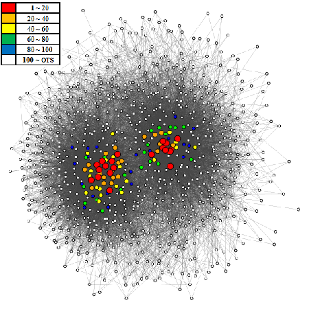
In Figure 3, we show the distribution of ranking by and . Same as Figure 1, theta has the same effect for gathering node in the middle of graphs. In addition, we can observe that the hitmen by setting and are slightly different from ranking by . The reason is that when we have the information from our neighbors’ neighbor, some messages that our neighbors are unwilling to tell may be revealed. Therefore, these hidden hitmen will emerge due to the exposure of these secret messages. More details are provided in Table II.
In Table II, the values for the three Jaccard indexes we proposed are listed. As the theta increases, the positive Jaccard index does increase as a very similar way as listed in Table I. However, the positive Jaccard index in Table I is one when is 0.2878 and the positive Jaccard index is one when is one. We can find if we consider the path which length is two, the positive Jaccard index converges slowly. It is because we have to consider more information than only consider the path which length is one. The obvious difference is that the negative Jaccard index values are much lower compared to the result that only consider the path which length is one. Due to the fact that when considering not just the neighbors of a node but both its neighbors and its neighbors’ neighbors, we would get more information and thus find a more global ranking. The negative Jaccard index and the total Jaccard index have very similar changes of behavior as the positive Jaccard index when considering the path which length is two. To study more about the difference between these two path sampling, Figure 4 provides more graphical details.
For the negative Jaccard index, it is relatively lower compared to the result of considering the path which length is one in Figure 4. Since considering the path which length is two would consider two edges rather than one, it means that there will be four circumstances to consist a two-step edge pair including negative/negative, negative/positive, positive/negative and positive/positive. We have to consider the positive/negative and negative/positive edge pairs to figure out the negative Jaccard index. Therefore, the lower negative Jaccard index has been generated. In the same way, we have to add the positive/positive and negative/negative edge pairs into our consideration for the calculation of the positive Jaccard index. We also look forward to a relatively lower positive Jaccard index when is not too large same as the negative Jaccard index does. However, there are only 8.5% of negative edges in this network such that the influence of negative edges can be ignored. As a result, the positive Jaccard index acts in the same way as it does in considering the path which length is only one when theta grows larger.
In opinion dynamic, we say that the spread of the information is a way to define centrality. Considering the path which length is only one provides a way to find the influence centrality for a node to its neighbors. Moreover, if we want to find the influence centrality for a node to those nodes which can not be reached in random walk only one step, we have to apply random walk more step to figure this out.
IV-B Experiment for trust centrality
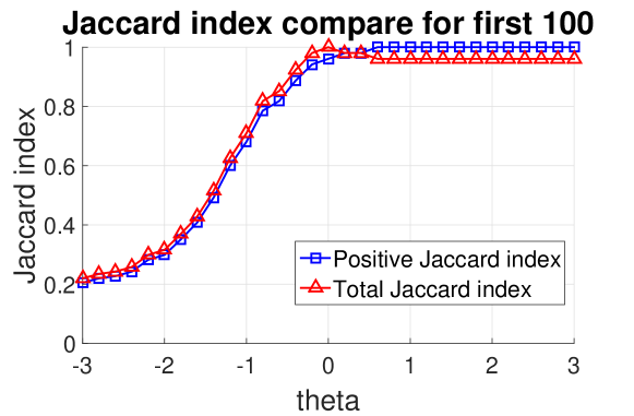
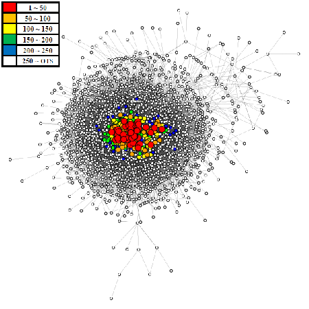
We use the same data as used in the experiment for influence centrality. In trust centrality, we have to consider the path which length is two because if only considering the path which length is one the result is as same as the influence centrality considering only the path which length is one. In Figure 5, no matter how we adjust theta, figure (a), (b) and (c) look similar. It is because the higher ranking node has more positive edges in trust centrality, and we have to consider positive/positive edges in two-step approach. Then in this dataset, the positive edges accounted for 91.5%. When theta is closer to zero, the rank is more similar to rank by total edges. When theta is larger, the rank is more similar to rank by positive edges. It is different from Figure 4.
In Figure 4, the line of positive Jaccard index slowly close to one when theta is larger. It is because it has to consider the negative/negative and positive/positive edges. In Figure 6, we only have to consider positive/positive edges, so the line is equal to one when theta is larger. It is as same as the line in Figure 2. With the increase of theta, we can find who is worthy of our trust. It is our definition of trust centrality.
|

|
|
| (a) =0 | (b) =0.05 | (c) =0.1 |
IV-C Experiment for advertisement-specific influence centrality
We evaluate our model on MemeTracker dataset [24], which tracks the quotes and phrases that frequently appear over time across mass media and personal blogs. Each cascade is composed of a ”meme’ (the phrase being mentioned), and the timestamps records of sites which have mentioned that phrase. To get advertisement information from these memes, we leverage Carrot2 [25], an open source clustering engine, with STC clustering algorithm to classify memes into fifteen topics including People, Going, Know, Years, Way, United States, States, Life, Believe, Lot, Love, America, Country, Barack Obama and Obama. For the data-independency purpose, we delete United States and Barack Obama since they are subsets of topic States and Obama. Therefore, we obtain a dataset with thirteen regularly-used phrases in it. Before we rank these nodes, we have to delete the nodes with degree smaller than 7 and self-loop edges, that is, their ranks are not important. As a result, we obtain the attributed network containing 2082 nodes and 16,503 edges.
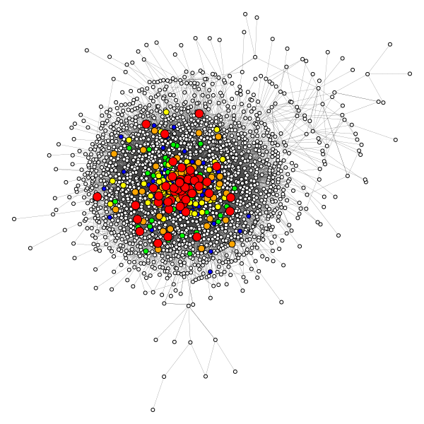
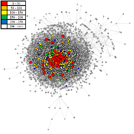
We choose the phrase ”Going” as an advertisement and input it into the existing attributed network that has node attribute. Since the ranking results by the sampling with path length 1 and the sampling with path length 2 are almost the same, we simply use the rank of sampling with path length 1 to do performance evaluation. Then, treating the advertisement as a sampling bias to find the pass measure and plot it as Figure 7 varying with . As so, it is obvious to see that the red nodes with higher rank gradually gather in the middle of the graph while slowly decrease down to zero. Then, we use Jaccard index for more detail explanation.
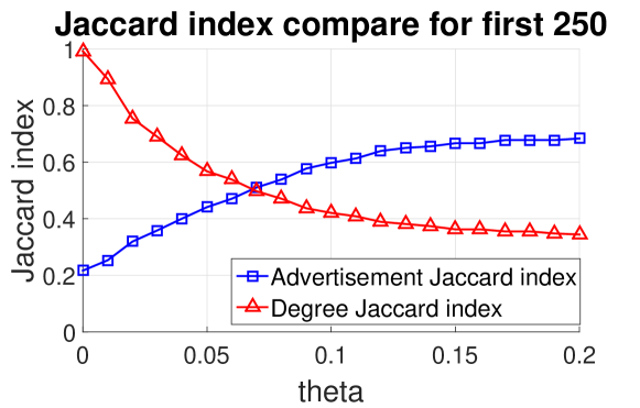
In this paper, we simply call the Jaccard index between the rank of degree and the rank generated by setting as Degree Jaccard index. Also, we call the Jaccard index between the rank of the regularly-used phrases and rank generated by setting the as Advertisement Jaccard index. In Figure 8, we show the relationship between and the two Jaccard index respectively. Degree Jaccard index has an escalating trend while is close to zero. On the other hand, Advertisement Jaccard index raises up as grows large, we claim it as advertisement-specific influence centrality. Then, the smaller the is, the more similar the ranking is to the rank of degree. On the contrary, if the increases, the rank would be more relevant to the rank of advertisement.
|

|
|
| (a) Going | (b) Know | (c) People |
|

|
|
| (a) Years | (b) America | (c) Obama |
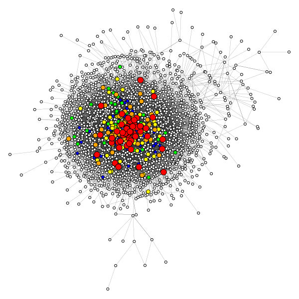
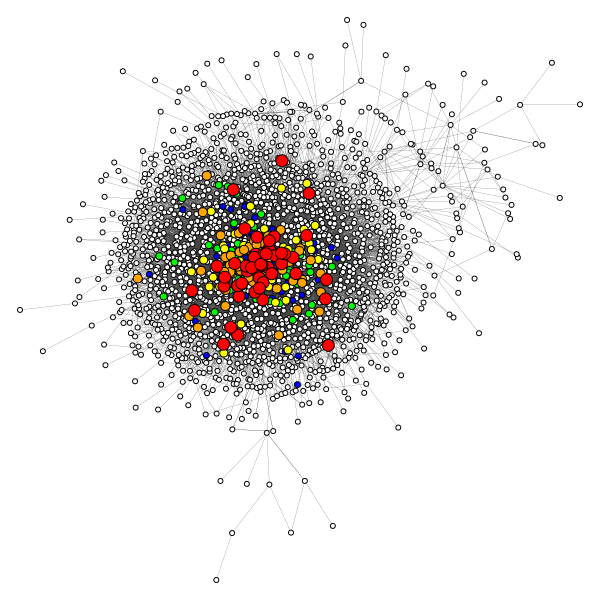
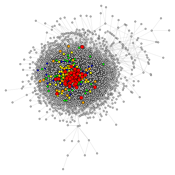
For experimental settings, we set as 0.2 because the top 250 nodes do not change by increasing the over than 0.2. Then we choose the top six most frequently-used phrases as test data, including Going, Know, People, Years, America, and Obama. We apply each phrase to our algorithm one by one and find that the top rank nodes are not in complete accord. Figure 9 leads to the fact that the top rank nodes may not be the same between any two topics.

|

|
| (a) Going and Obama | (b) Know and America |
Besides, we combine advertisements from different aspects and do the performance evaluation to find the top rank node of these advertisements. In Figure 10, figure (a) is combined by two advertisements that is ”Going” and ”Obama,” and figure (b) is combined by the advertisement ”Know” and the advertisement ”America”. The result is not necessarily the same compared to the result of each advertisement we used to combine in.
As a result, if there is an advertisement containing all sort of contents and we would like to know who is the most influential person to it in the existing network, we can get the answer through this experiment. Briefly speaking, we pick up those important phrases in the contents manually and apply them to our algorithms. Thus, those nodes which are truly beneficial to the promotion for the advertisement can be found out. This may be very different to the fact that people usually think the higher degree a node has the more value the node can create for an advertisement.
V Conclusion
In this paper, we extend our previous work in [16] to attributed networks. Our approach is to extend the bivariate distributions in an unsigned network to a signed network by using the exponential change of measure. Hence, the centrality is also being separated into three different terms of centrality which are the positive influence centrality, negative influence centrality, and the total influence centrality. Besides, the experimental results also help us learn the relationship between temperature (theta) and the three centralities. We also would like to extend this definition to community detection and not just using it as centrality.
References
- [1] L. C. Freeman, “A set of measures of centrality based on betweenness,” Sociometry, pp. 35–41, 1977.
- [2] M. Newman, Networks: an introduction. Oxford university press, 2010.
- [3] L. C. Freeman, “Centrality in social networks conceptual clarification,” Social networks, vol. 1, no. 3, pp. 215–239, 1978.
- [4] P. J. Mucha, T. Richardson, K. Macon, M. A. Porter, and J.-P. Onnela, “Community structure in time-dependent, multiscale, and multiplex networks,” science, vol. 328, no. 5980, pp. 876–878, 2010.
- [5] S. Boyd, A. Ghosh, B. Prabhakar, and D. Shah, “Gossip algorithms: Design, analysis and applications,” in INFOCOM 2005. 24th Annual Joint Conference of the IEEE Computer and Communications Societies. Proceedings IEEE, vol. 3. IEEE, 2005, pp. 1653–1664.
- [6] C.-S. Chang, C.-Y. Hsu, J. Cheng, and D.-S. Lee, “A general probabilistic framework for detecting community structure in networks,” in INFOCOM, 2011 Proceedings IEEE. IEEE, 2011, pp. 730–738.
- [7] L. Page, S. Brin, R. Motwani, and T. Winograd, “The pagerank citation ranking: Bringing order to the web.” Stanford InfoLab, Tech. Rep., 1999.
- [8] V. Latora and M. Marchiori, “A measure of centrality based on network efficiency,” New Journal of Physics, vol. 9, no. 6, p. 188, 2007.
- [9] E. Estrada and J. A. Rodriguez-Velazquez, “Subgraph centrality in complex networks,” Physical Review E, vol. 71, no. 5, p. 056103, 2005.
- [10] A. Mohammadinejad, R. Farahbakhsh, and N. Crespi, “Employing personality feature to rank the influential users in signed networks,” in Big Data and Cloud Computing (BDCloud), Social Computing and Networking (SocialCom), Sustainable Computing and Communications (SustainCom)(BDCloud-SocialCom-SustainCom), 2016 IEEE International Conferences on. IEEE, 2016, pp. 346–353.
- [11] H. Kim and R. Anderson, “Temporal node centrality in complex networks,” Physical Review E, vol. 85, no. 2, p. 026107, 2012.
- [12] D. Taylor, S. A. Myers, A. Clauset, M. A. Porter, and P. J. Mucha, “Eigenvector-based centrality measures for temporal networks,” Multiscale Modeling & Simulation, vol. 15, no. 1, pp. 537–574, 2017.
- [13] J. Jung, W. Jin, L. Sael, and U. Kang, “Personalized ranking in signed networks using signed random walk with restart,” in Data Mining (ICDM), 2016 IEEE 16th International Conference on. IEEE, 2016, pp. 973–978.
- [14] J. Weng, E.-P. Lim, J. Jiang, and Q. He, “Twitterrank: finding topic-sensitive influential twitterers,” in Proceedings of the third ACM international conference on Web search and data mining. ACM, 2010, pp. 261–270.
- [15] C.-S. Chang, C.-J. Chang, W.-T. Hsieh, D.-S. Lee, L.-H. Liou, and W. Liao, “Relative centrality and local community detection,” Network Science, vol. 3, no. 4, pp. 445–479, 2015.
- [16] C.-S. Chang, D.-S. Lee, L.-H. Liou, S.-M. Lu, and M.-H. Wu, “A probabilistic framework for structural analysis in directed networks,” in Communications (ICC), 2016 IEEE International Conference on. IEEE, 2016, pp. 1–6.
- [17] S. Brin and L. Page, “Reprint of: The anatomy of a large-scale hypertextual web search engine,” Computer networks, vol. 56, no. 18, pp. 3825–3833, 2012.
- [18] M. Rosvall and C. Bergstrom, “Maps of information flow reveal community structure in complex networks,” arXiv preprint physics.soc-ph/0707.0609, 2007.
- [19] R. Lambiotte, J.-C. Delvenne, and M. Barahona, “Random walks, markov processes and the multiscale modular organization of complex networks,” IEEE Transactions on Network Science and Engineering, vol. 1, no. 2, pp. 76–90, 2014.
- [20] T. M. Cover and J. A. Thomas, Elements of information theory. John Wiley & Sons, 2012.
- [21] C.-S. Chang, Performance guarantees in communication networks. Springer Science & Business Media, 2012.
- [22] S. Juneja and P. Shahabuddin, “Rare-event simulation techniques: an introduction and recent advances,” Handbooks in operations research and management science, vol. 13, pp. 291–350, 2006.
- [23] L. A. Adamic and N. Glance, “The political blogosphere and the 2004 us election: divided they blog,” in Proceedings of the 3rd international workshop on Link discovery. ACM, 2005, pp. 36–43.
- [24] J. Leskovec, L. Backstrom, and J. Kleinberg, “Memetracker data,” 2008.
- [25] S. Osiński and D. Weiss, “Carrot2: Design of a flexible and efficient web information retrieval framework,” in International atlantic web intelligence conference. Springer, 2005, pp. 439–444.