Self-Supervised Learning for Spinal MRIs

Abstract

A significant proportion of patients scanned in a clinical setting have follow-up scans. We show in this work that such longitudinal scans alone can be used as a form of “free” self-supervision for training a deep network. We demonstrate this self-supervised learning for the case of T2-weighted sagittal lumbar Magnetic Resonance Images (MRIs). A Siamese convolutional neural network (CNN) is trained using two losses: (i) a contrastive loss on whether the scan is of the same person (i.e. longitudinal) or not, together with (ii) a classification loss on predicting the level of vertebral bodies. The performance of this pre-trained network is then assessed on a grading classification task. We experiment on a dataset of 1016 subjects, 423 possessing follow-up scans, with the end goal of learning the disc degeneration radiological gradings attached to the intervertebral discs. We show that the performance of the pre-trained CNN on the supervised classification task is (i) superior to that of a network trained from scratch; and (ii) requires far fewer annotated training samples to reach an equivalent performance to that of the network trained from scratch.

1 Introduction

A prerequisite for the utilization of machine learning methods in medical image understanding problems is the collection of suitably curated and annotated clinical datasets for training and testing. Due to the expense of collecting large medical datasets with the associated ground-truth, it is important to develop new techniques to maximise the use of available data and minimize the effort required to collect new cases.

In this paper, we propose a self-supervision approach that can be used to pre-train a CNN using the embedded information that is readily available with standard clinical image data. Many patients are scanned multiple times in a so-called longitudinal manner, for instance to assess changes in disease state or to monitor therapy. We define a pre-training scheme using only the information about which scans belong to the same patient. Note, we do not need to know the identity of the patient; only which images belong to the same patient. This information is readily available in formats such as DICOM (Digital Imaging and Communications in Medicine) that typically include a rich set of meta-data such as patient identity, date of birth and imaging protocol (and DICOM anonymization software typically assigns the same ‘fake-id’ to images of the same patient).

Here, we implement this self-supervision pre-training for the case of T2-weighted sagittal lumbar MRIs. We train a Siamese CNN to distinguish between pairs of images that contain the same patient scanned at different points in time, and pairs of images of entirely different patients. We also illustrate that additional data-dependent self-supervision tasks can be included by specifying an auxiliary task of predicting vertebral body levels, and including both types of self-supervision in a multi-task training scheme. Following the pre-training, the learned weights are transferred to a classification CNN that, in our particular application of interest, is trained to predict a range of gradings related to vertebra and disc degeneration. The performance of the classification CNN is then used to evaluate the success of the pre-training. We also compare to pre-training a CNN on a large dataset of lumbar T2-weighted sagittal MRIs fully annotated with eight radiological gradings [5].

Related Work: Models trained using only information contained within an image as a supervisory signal have been proven to be effective feature descriptors e.g. [4] showed that a CNN trained to predict relative location of pairs of patches, essentially learning spatial context, is better at a classification task (after fine-tuning) then a CNN trained from scratch. The task of learning scans from the same unique identity is related to slow-feature learning in videos [7, 10, 11].

Transfer learning in CNNs has been found to be extremely effective especially when the model has been pre-trained on a large dataset like ImageNet [3], and there have been several successes on using models pre-trained on natural images on medical images e.g.  lung disease classification [8]. However, since a substantial portion of medical images are volumetric in nature, it is also appropriate to experiment with transfer learning with scans of the same modality rather than using ImageNet-trained models.

2 Self-Supervised Learning

This section first describes the details of the input volumes extraction: the vertebral bodies (VBs) that will be used for the self-supervised training; and the intervertebral discs (IVDs) that will be used for the supervised classification experiments. We then describe the loss functions and network architecture.

2.1 Extracting Vertebral Bodies and Intervertebral Discs

For each T2-weighted sagittal MRI we automatically detect bounding volumes of the (T12 to S1) VBs alongside the level labels using the pipeline outlined in [5, 6]. As per [5], we also extract the corresponding IVD volumes (T12-L1 to L5-S1, where T, L, and S refer to the thoracic, lumbar, and sacral vertebrae) from the pairs of vertebrae e.g. a L5-S1 IVD is the disc between the L5 and S1 vertebrae. Fig. 1 shows the input and outputs of the extraction pipeline. The slices of both the VB and IVD volumes are mid-sagittally aligned (to prevent misalignment that can occur from scoliosis and other disorders) and zero-padded slice-wise if the number of slices is below the predefined 9 channels. The volumes are rescaled according to the width of the VB or IVD and normalized such that the median intensity of the VB above and below the current VB or IVD is $0.5$.

Figure 1: Extracting VB and IVD Volumes: For each MRI, we extract 7 VB (T12 to S1) and 6 IVD (T12-L1 to L5-S1) volumes. The dimensions of the volumes are: (i) $224\times 224\times 9$ for the VBs, and (ii) $112\times 224\times 9$ for the IVDs. The whole volume is centred at the detected middle slice of the volume of the VB/IVD.

2.2 Longitudinal Learning via Contrastive Loss

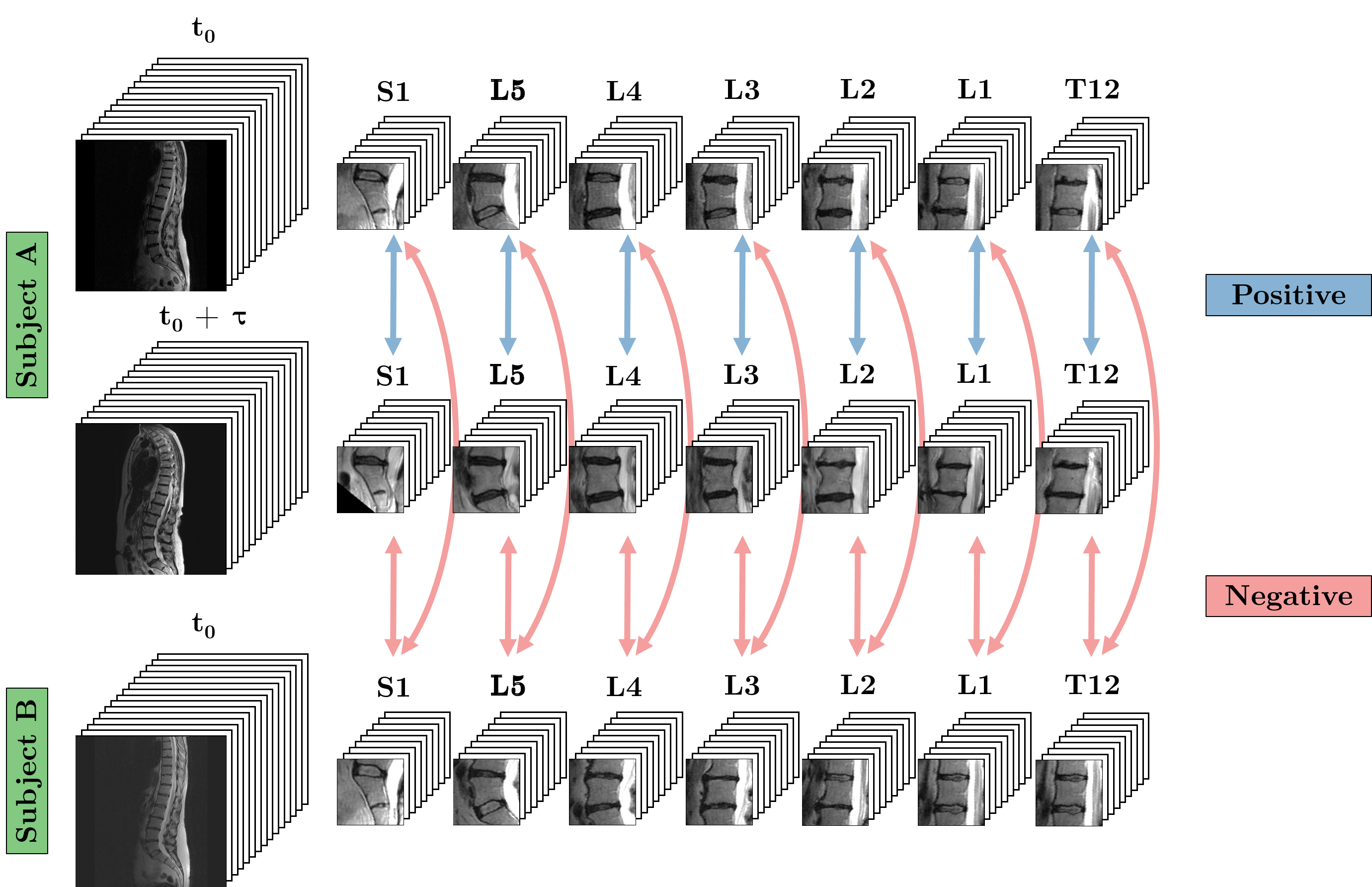
The longitudinal information of the scans is used to train a Siamese network such that the embeddings for scans of the same person are close, whereas scans of different people are not. The input is a pair of VBs of the same level; an S1 VB is only compared against an S1 VB and vice versa. We use the contrastive loss in [2], $\mathcal{L}_{C}=\sum_{n=1}^{N}(y)d^{2}+(1-y)\max(0,m-d)^{2}$, where $d=\|a_{n}-b_{n}\|_{2}$, and $a_{n}$ and $b_{n}$ are the 1024-dimensional FC7 (embedding) vectors for the first and second VB in an input pair, and $m$ is a predefined margin. Positive, $y=1$, VB pairs are those that were obtained from a single unique subject (same VB scanned at different points in time) and negative, $y=0$, pairs are VBs from different individuals (see Fig. 3).

We use the VBs instead of the IVDs due to the fact that vertebrae tend to be more constant in shape and appearance over time. Fig. 2 shows examples of both VB and IVD at different points in time. In other medical tasks the pair of VBs can easily be changed to other anatomies for example comparing lungs in chest X-rays.

Figure 2: VB and IVD Across Time: The VB appears unchanged but over time the IVD loses intensity of its nucleus and experiences a loss in height. Furthermore, in the IVD example, we can observe a vertebral slip, or spondylolisthesis, which does not change the appearance of the VBs themselves but significantly changes the IVD.

Figure 3: Generating the positive/negative pairs: The arrows mark a pair of VBs, where blue arrows highlight positive pairs while negative are highlighted in red. Each pair is generated from two scans. $\mathbf{t_{0}}$ refers to the time of the initial scan and $\boldsymbol{\uptau}$ is the time between the baseline and the follow-up scans, typically 10 years in our dataset.

2.3 Auxiliary Loss – Predicting VB Levels

In addition to the contrastive loss, we also employ an auxiliary loss to give complementary supervision. Since each VB pair is made up of VBs of the same level, we train a classifier on top of the FC7 layer, i.e. the discriminative layer, to predict the seven levels of the VB (from T12 to S1). The overall loss can then be described as a combination of the contrastive and softmax log losses, $\mathcal{L}=\mathcal{L}_{C}-\sum_{n=1}^{N}\alpha_{c}\left(y_{c}(x_{n})-\log\sum_{j=1}^{7}e^{y_{j}(x_{n})}\right)$, where $y_{j}$ is the $j$th component of the FC8 output, $c$ is the true class of $x_{n}$, and $\alpha_{c}$ is the class-balanced weight as in [5].

2.4 Architecture

The base architecture trained to distinguish VB pairs is based of the VGG-M network in [1] (see Fig. 4). The input to the Siamese CNN is the pairs of VBs, with dimension $224\times 224\times 9$. We use 3D kernels from Conv1 to Conv4 layers followed by a 2D Conv5. To transform the tensor to be compatible with 2D kernels, the Conv4 kernel is set to be $3\times 3\times 9$ with no padding, resulting in a reduction of the slice-wise dimension after Conv4. We use $2\times 2$ max pooling. The output dimension of the FC8 layer depends on the number of classes i.e. seven for the self-supervisory auxiliary task of predicting the seven VB levels.

Figure 4: The Siamese network architecture is trained to distinguish between VB pairs from the same subject (same VB scanned a decade apart) or VB pairs from different subjects. There is also an additional loss (shown as aux) to predict the level of the VB.

3 Dataset & Implementation Details

We experimented on a dataset of 1016 recruited subjects (predominantly female) from the TwinsUK registry (www.twinsuk.ac.uk) not using backpain as an exclusion or selection criterion. As well as a baseline scan for each subject, 423 subjects have follow-up scans taken 8-12 years after the original baseline. A majority of the subjects with the follow-up scans have only two scans (one baseline and one follow-up) while a minority have three (one baseline and two follow-up). The baseline scans were taken with a 1.0-Tesla scanner while the follow-up scans were taken with a 1.5-Tesla machine but both adhered to the same scanning protocol (slice thickness, times to recovery and echo, TR and TE). Only T2-weighted sagittal scans were collected for each subject.

3.1 Radiological Gradings

The subjects were graded with a measure of Disc Degeneration, not dissimilar to Pfirrmann Grading. The gradings were annotated by a clinician and were done on a per disc basis: from L1-L2 to L5-S1 discs (5 discs per subject). We use these gradings to assess the benefits of pre-training a classification network on longitudinal information. Examples of the gradings can be seen in Fig. 5. 920 of the 1016 subjects are graded.

Figure 5: Disc Degeneration: A four-class grading system based on Pfirrmann grading that depends on the intensity and height of the disc.

3.2 Training

Data augmentation: The augmentation strategies are identical to that described in [5] for the classification CNN while we use slightly different augmentations to train the Siamese network. The augmentations are: (i) rotation with $\theta$ = $-15^{\circ}$ to $15^{\circ}$, (ii) translation of $\pm 48$ pixels in the x-axis, $\pm 24$ pixels in the y-axis, $\pm 2$ slices in the z-axis, (iii) rescaling with a scaling factor between $90\%$ to $110\%$, (iv) intensity variation $\pm 0.2$, and (v) random slice-wise flip i.e. reflection of the slices across the mid-sagittal (done on a per VB pair basis).

Details: Our implementation is based on the MatConvNet toolbox [9] and the networks were trained using an NVIDIA Titan X GPU. The hyperparameters are: batch size 128 for classification and 32 for the Siamese network; momentum 0.9; weight decay 0.0005; learning rate $1e^{-3}$ (classification) and $1e^{-5}$ (self-supervision) and lowered by a factor of 10 as the validation error plateaus, which is also our stopping criterion, normally around 2000 epochs for the classification network and 500 epochs for the Siamese network.

4 Experiments & Results

4.1 Longitudinal Learning & Self-supervision

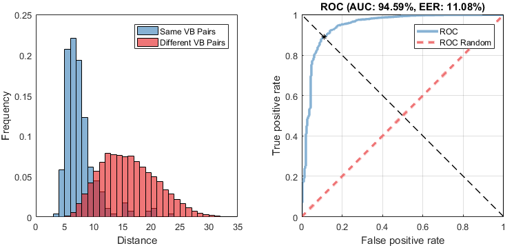
The dataset is split by subject 80:10:10 into train, validation, and test sets. For the 423 subjects with multiple scans this results in a 339:42:42 split. Note, a pair of twins will only be in one set i.e. one subject part of a twin pair can’t be in training and the other in test. With the trained network, each input VB can be represented as a 1024-dimensional FC7 vector. For each pair of VBs i.e. two FC7 vectors, we can calculate the $L_{2}$ distance between two samples, which is the same distance function used during training. Fig. 6 shows the histogram of the distances (both positive and negative) for all the VB pairs in the test set. In general, VB pairs that are from the same subject have lower distances compared to pairs from different subjects. Using the distances between pairs as classification scores of predicting whether the VB pairs are from the same or different subjects, we achieve an AUC of $\mathbf{94.6}$%. We also obtain a very good performance of $\mathbf{97.8}$% accuracy on the auxiliary task of predicting VB level.

Figure 6: Left: Histogram of VB pairs distances in the test set. Positive pairs in blue, negative in red. Right: The ROC of the classification of positive/negative VB pairs.

4.2 Benefits of Pre-training

To measure the performance gained by pre-training using the longitudinal information we use the convolution weights learnt in the Siamese network, and train a classification CNN to predict the Disc Degeneration radiological grading (see Fig. 7). For this classification task we use the 920 subjects that possess gradings and split them into the following sets: 670 for training, 50 in validation, and 200 for testing. Subjects with follow-up scans ($>1$ scans) are only used in training and not for testing so, in essence, the Siamese network will never have seen the subjects in the classification test set.

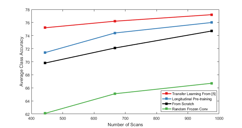
We transfer and freeze convolutional weights of the Siamese network and only train the randomly-initialized fully-connected layers. We also experimented with fine-tuning the convolutional layers but we find the difference in performance to be negligible. For comparison, we also train: (i) a CNN from scratch, (ii) a CNN with a frozen randomly initialized convolutional layers (to see the power of just training on the fully-connected layers) as a baseline, and (iii) a CNN using convolutional weights of a CNN trained on a fully-annotated spinal MRI dataset with multiple radiological gradings in [5]. The performance measure is the average class accuracy, calculated as the average of the diagonal elements of the normalized confusion matrix.

Figure 7: The architecture of the classification CNN. The convolutional weights are obtained from the Siamese network.

Fig. 8 shows the performance of all the models as the number of training samples is varied at [240, 361, 670] subjects or [444, 667, 976] scans. It can be seen that with longitudinal pre-training, less data is required to reach an equivalent point to that of training from scratch, e.g. the performance is $\mathbf{74.4}$% using only 667 scans by pre-training, whereas training from scratch requires 976 scans to get to $\mathbf{74.7}$%. This performance gain can also be seen with a lower amount of training data. As would be expected, transfer learning from a CNN trained with strong supervision using the data in [5] is better, with an accuracy at least $\mathbf{2.5}$% above training from scratch. Unsurprisingly, a classifier trained on top of fully random convolutional weights performs the worst.

Figure 8: Accuracy as the number of training samples for IVD classification is increased. Longitudinal pre-training improves over training from scratch, showing its benefit, and this performance boost persists even at 976 scans. Transfer learning from a CNN trained on a strongly-supervised dataset (including IVD classification) is better and provides an ‘upper bound’ on transfer performance. Note, even with 976 scans in the training set, the performance has not plateaued hinting at further improvements with the availability of more data.

Since longitudinal information is essentially freely available when collecting data, the performance gain from longitudinal pre-training is also free. It is interesting to note that even though the Siamese network is trained on a slightly different input, VBs instead of IVDs, transferring the weights for classification task on IVDs still achieves better performance than starting from scratch. However, we suspect this difference in inputs is the primary reason why the performance gain is lower when the amount of training data is low as the network needs more data to adapt to the IVD input/task (in contrast, the strongly supervised CNN is trained on both VB and IVD classification).

5 Conclusion

We have shown that it is possible to use self-supervision to improve performance on a radiological grading classification task and we hope to explore the benefits of adding more auxiliary tasks in the near future e.g. predicting gender, age and weight. The performance improvement is nearing that of transfer learning from a model trained on a fully annotated dataset given that the target training set itself contains enough data. Furthermore, having a distance function between vertebral pairs opens up the possibility of identifying people using their MRIs.

Acknowledgements.

We are grateful for discussions with Prof. Jeremy Fairbank, Dr. Jill Urban, and Dr. Frances Williams. This work was supported by the RCUK CDT in Healthcare Innovation (EP/G036861/1) and the EPSRC Programme Grant Seebibyte (EP/M013774/1). TwinsUK is funded by the Wellcome Trust; European Community’s Seventh Framework Programme (FP7/2007-2013). The study also receives support from the National Institute for Health Research (NIHR) Clinical Research Facility at Guy’s & St Thomas’ NHS Foundation Trust and NIHR Biomedical Research Centre based at Guy’s and St Thomas’ NHS Foundation Trust and King’s College London.

References

- [1] Chatfield, K., Simonyan, K., Vedaldi, A., Zisserman, A.: Return of the devil in the details: Delving deep into convolutional nets. In: Proc. BMVC. (2014)
- [2] Chopra, S., Hadsell, R., LeCun, Y.: Learning a similarity metric discriminatively, with application to face verification. In: Proc. CVPR (2005)
- [3] Deng, J., Dong, W., Socher, R., Li, L.J., Li, K., Fei-Fei, L.: Imagenet: A large-scale hierarchical image database. In: Proc. CVPR (2009)
- [4] Doersch, C., Gupta, A., Efros, A.A.: Unsupervised visual representation learning by context prediction. In: Proc. ICCV (2015)
- [5] Jamaludin, A., Kadir, T., Zisserman, A.: Spinenet: Automatically pinpointing classification evidence in spinal mris. In: MICCAI (2016)
- [6] Lootus, M., Kadir, T., Zisserman, A.: Vertebrae detection and labelling in lumbar mr images. In: MICCAI Workshop: CSI (2013)
- [7] Mobahi, H., Collobert, R., Weston, J.: Deep learning from temporal coherence in video. In: ICML (2009)
- [8] Shin, H.C., Roth, H.R., Gao, M., Lu, L., Xu, Z., Nogues, I., Yao, J., Mollura, D., Summers, R.M.: Deep convolutional neural networks for computer-aided detection: Cnn architectures, dataset characteristics and transfer learning. IEEE Transactions on Medical Imaging 35(5), 1285–1298 (May 2016)
- [9] Vedaldi, A., Lenc, K.: Matconvnet – convolutional neural networks for matlab. CoRR abs/1412.4564 (2014)
- [10] Wang, X., Gupta, A.: Unsupervised learning of visual representations using videos. In: ICCV (2015)
- [11] Wiskott, L., Sejnowski, T.J.: Slow feature analysis: Unsupervised learning of invariances. Neural Computation 14(4), 715–770 (April 2002)