Learning the kernel matrix by resampling

Abstract

In this abstract paper, we introduce a new kernel learning method by a nonparametric density estimator. The estimator consists of a group of k-centroids clusterings. Each clustering randomly selects data points with randomly selected features as its centroids, and learns a one-hot encoder by one-nearest-neighbor optimization. The estimator generates a sparse representation for each data point. Then, we construct a nonlinear kernel matrix from the sparse representation of data. One major advantage of the proposed kernel method is that it is relatively insensitive to its free parameters, and therefore, it can produce reasonable results without parameter tuning. Another advantage is that it is simple. We conjecture that the proposed method can find its applications in many learning tasks or methods where sparse representation or kernel matrix is explored. In this preliminary study, we have applied the kernel matrix to spectral clustering. Our experimental results demonstrate that the kernel generated by the proposed method outperforms the well-tuned Gaussian RBF kernel. This abstract paper is used to protect the idea, full versions will be updated later.

I Introduction

Learning data representations is an important issue for machine learning. One type of data representations are produced by hand-crafted features, such as various kinds of filters and kernels. Another type are produced by density estimators, such as k-means, Gaussian mixture models, kernel learning, etc. This paper focuses on kernel methods. Common predefined kernel functions include the linear kernel, polynomial kernels, Gaussian RBF kernels, etc. Some kernel matrices are produced by density estimators, such as SDP or metric learning.

In this paper, we introduce a new kernel learning method, which generates a kernel matrix from a simple nonparametric density estimator. The estimator consists of a group of k-centroids clusterings. Each clustering randomly selects data points with randomly selected features as its centroids, and learns a one-hot encoder by one-nearest-neighbor optimization. The estimator generates a sparse representation for each data point. Then, the nonlinear kernel matrix is constructed from the sparse representation of data. One major advantage of the proposed kernel method is that it can produce reasonable result without parameter tuning, compared to traditional nonlinear kernels, such as Gaussian RBF. Another advantage is that it is simple. We believe that the proposed method can find its applications in many learning tasks or methods where sparse representation or kernel matrix is explored, such as unsupervised learning, semisupervised learning, supervised learning. In this initial study, we have applied the kernel matrix to spectral clustering. Our experimental results demonstrate that the kernel generated by the proposed method outperforms the well-tuned Gaussian RBF kernel.

II Method

Given a $d$-dimensional input data set $\mathcal{X}=\left\{\mathbf{x}_{1},\ldots,\mathbf{x}_{n}\right\}$, the method trains $V$ ($V\gg 1$) $k$-centroids clusterings. For training each layer either from the lower layer or from the original data space, we simply need to focus on training each $k$-centroids clustering, which consists of the following three steps:

• Random feature selection. The first step randomly selects $\hat{d}$ dimensions of $\mathcal{X}$ ($\hat{d}\leq d$) to form a subset of $\mathcal{X}$, denoted as $\hat{\mathcal{X}}=\left\{\hat{\mathbf{x}}_{1},\ldots,\hat{\mathbf{x}}_{n}\right\}$.

• Random sampling. The second step randomly selects $k=\lfloor\delta n\rfloor$ data points from $\hat{{\mathcal{X}}}$ as the $k$ centroids of the clustering, denoted as $\{\mathbf{w}_{1},\ldots,\mathbf{w}_{k}\}$, where $\delta\in(0,1)$ is a free parameter.

• Sparse representation learning. The third step assigns each input data point $\hat{\mathbf{x}}$ to one of the $k$ clusters and outputs a $k$-dimensional indicator vector $\mathbf{h}=[h_{1},\ldots,h_{k}]^{T}$, where operator ^T denotes the transpose of vector. For example, if $\hat{\mathbf{x}}$ is assigned to the second cluster, then $\mathbf{h}=[0,1,0,\ldots,0]^{T}$. The assignment is calculated according to the similarities between $\hat{\mathbf{x}}$ and the $k$ centroids, in terms of some predefined similarity metric at the original data space, such as the squared Euclidean distance $\arg\min_{i=1}^{k}\|\mathbf{w}_{i}-\hat{\mathbf{x}}\|^{2}$, or in terms of $\arg\max_{i=1}^{k}\mathbf{w}_{i}^{T}\hat{\mathbf{x}}$ at all other hidden layers.

• Kernel matrix construction. The last step constructs the similarity matrix ${\mathbf{K}}$ by $K_{i,j}={\mathbf{x}}^{T}_{i}{\mathbf{x}}_{j},\forall i=1,\ldots,n\mbox{ and }\forall j=1,\ldots,n$. It is obvious that ${\mathbf{K}}$ is a kernel matrix.

III Applications

We apply the kernel matrix to spectral clustering [1]. To prevent the local minima of $k$-means clustering in spectral clustering, we run the $k$-means clustering multiple times (in this paper, 50 times), and pick the clustering result that corresponds to the lowest objective value among the candidate objective values as the final clustering result of the spectral clustering.

IV Experiments

The data sets for evaluation were summarized in Table I. For each data set, we ran the spectral clustering 10 times and reported the average performance. The clustering results were evaluated by NMI and clustering accuracy (ACC).

We compared the proposed method with the RBF kernel based spectral clustering. For the proposed method, parameter $\delta$ was searched in grid through $[0.1:0.1:0.9]$ where the symbol $[A:b:C]$ denotes a set of numbers starting from $A$ and ending by $C$ with an interval of $b$; parameter $a$ was fixed to $0.5$; parameter $V=400$. For the Gaussian RBF kernel, the kernel width $\sigma$ was set from $2^{[-4:1:4]}A$ where $A$ is the average of the pairwase Euclidean distances between data points.

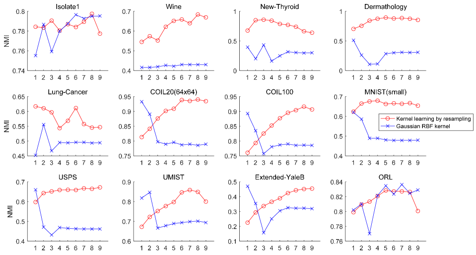
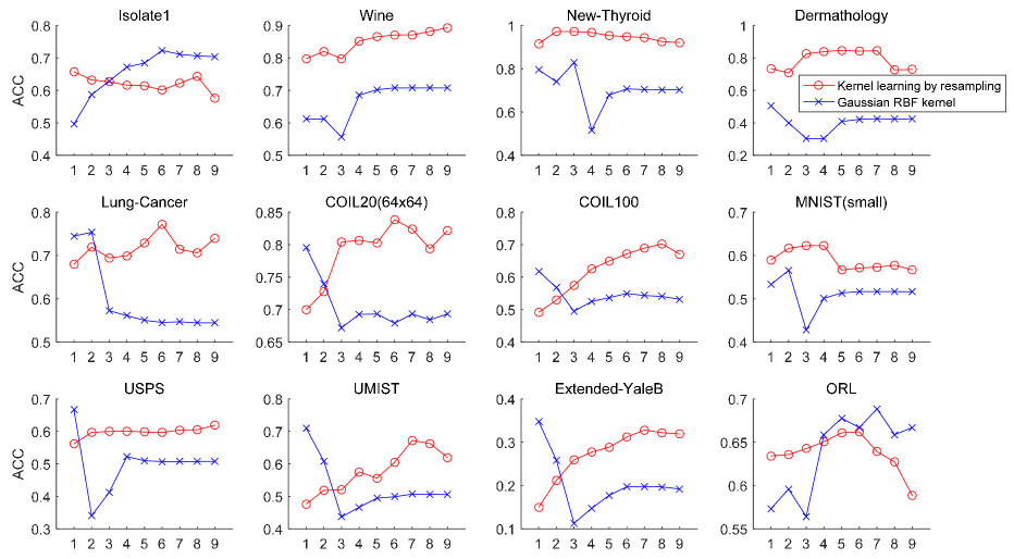
Experimental comparison results with the Gaussian RBF kernels are shown in Figs. 1 and 2. From the figures, we can see that, the proposed method generally reaches the optimal performance when $\delta\in[0.6,0.8]$. This empirical conclusion is invalid apparently only on “New-Thyroid” and “Lung-Cancer”. On the other side, the Gaussian RBF kernel reaches the optimal performance when $\sigma\in[2^{-4}A,2^{-3}A]$, and this empirical conclusion is invalid apparently on “Isolate1” and “ORL”.

For unsupervised learning and clustering, because we usually do not have prior knowledge on selecting optimal free parameters, we have to fix the free parameters without manual tuning. Here, we selected $\delta=0.7$ for the proposed method, and $\sigma=2^{-4}A$ for the Gaussian RBF kernel. The comparison results were summarized in Tables II and III where the best performance with the optimal free parameters was also reported. The statistical difference was evaluated by the two-tailed $t$-test where the $p$-value was set to $0.05$. Comparison results show that, given the free parameters that are no matter fixed or well-tuned, the proposed method outperforms the Gaussian RBF kernel in most of the data sets, particularly in terms of NMI.

We also compared the proposed method with $\delta$ fixed to 0.7 with the well-tuned Gassian RBF kernel. From the comparison results in Tables IV and V, we found that the the proposed method even without parameter tuning is comparable the well-tuned Gassian RBF kernel.

TABLE I: Description of data sets.

ID Name # data points # dimensions # classes Attribute 1 Isolet1 1560 617 26 Speech data 2 Wine 178 13 3 Chemical data 3 New-Thyroid 215 5 3 Biomedical data 4 Dermathology 366 34 6 Biomedical data 5 Lung-Cancer 203 12600 5 Biomedical data 6 COIL20(64x64) 1440 4096 20 Images 7 COIL100 7200 1024 100 Images 8 MNIST(small) 5000 768 10 Images (handwritten digits) 9 USPS 11000 1024 10 Images (handwritten digits) 10 UMIST 575 1024 20 Images (faces) 11 Extended-YaleB 2414 1024 38 Images (faces) 12 ORL 400 1024 40 Images (faces)

Figure 1: NMI Comparison of the proposed method and the Gaussian RBF kernel. Note that X-axis consists of the indices of the free parameters of either the proposed method or the Gaussian kernel. For the proposed method, the numbers $1,2,\ldots,9$ indexes the values $0.1,0.2,\ldots,0.9$ of the free parameter $\delta$ respectively. For the Gaussian RBF kernel, the numbers $1,2,\ldots,9$ indexes the values $2^{-4}A,2^{-3}A,\ldots,2^{4}A$ of the free parameter $\sigma$ respectively.

Figure 2: ACC Comparison of the proposed method and the Gaussian RBF kernel.

TABLE II: NMI on 12 data sets. The number after the symbol $\pm$ is the standard deviation.

$k$-means $k$-means+PCA Spectral+Gaussian_kernel^no_tuning Proposed^no_tuning Spectral+Gaussian_kernel^optimal Proposed^optimal 1 Isolet1 77.21%$\pm$0.92% 56.74%$\pm$0.75% 75.51%$\pm$0.58% 78.93%$\pm$0.44% 79.66%$\pm$0.58% 79.74%$\pm$0.39% 2 Wine 42.88%$\pm$0.00% 40.92%$\pm$0.00% 41.58%$\pm$0.00% 63.94%$\pm$0.00% 43.02%$\pm$0.00% 68.36%$\pm$0.00% 3 New-Thyroid 49.46%$\pm$0.00% 49.46%$\pm$ 0.00% 39.63%$\pm$0.00% 74.08%$\pm$0.00% 43.20%$\pm$0.00% 85.91%$\pm$0.00% 4 Dermathology 9.11%$\pm$0.11% 59.50%$\pm$0.10% 51.04%$\pm$0.15% 88.61%$\pm$0.00% 51.04%$\pm$0.15% 89.42%$\pm$0.00% 5 Lung-Cancer 48.59%$\pm$1.07% 49.17%$\pm$ 0.96% 45.18%$\pm$4.60% 55.70%$\pm$0.00% 55.58%$\pm$4.60% 61.70%$\pm$0.00% 6 COIL20(64x64) 78.03%$\pm$1.14% 79.00%$\pm$1.35% 93.29%$\pm$0.81% 93.54%$\pm$1.26% 93.29%$\pm$0.81% 93.97%$\pm$0.83% 7 COIL100 76.98%$\pm$0.27% 69.64%$\pm$0.45% 89.28%$\pm$0.59% 90.45%$\pm$0.25% 89.28%$\pm$0.59% 91.58%$\pm$0.52% 8 MNIST(small) 49.69%$\pm$0.14% 27.86%$\pm$0.08% 62.06%$\pm$0.04% 66.30%$\pm$0.01% 62.06%$\pm$0.04% 67.94%$\pm$0.01% 9 USPS 43.63%$\pm$1.78% 43.00%$\pm$0.05% 66.05%$\pm$2.38% 66.75%$\pm$0.84% 66.05%$\pm$0.18% 67.21%$\pm$0.28% 10 UMIST 65.36%$\pm$1.21% 66.25%$\pm$1.10% 81.83%$\pm$0.58% 85.88%$\pm$1.65% 84.66%$\pm$2.38% 85.88%$\pm$1.65% 11 Extended-YaleB 12.71%$\pm$0.63% 16.54%$\pm$0.56% 47.11%$\pm$0.58% 44.30%$\pm$0.72% 47.11%$\pm$0.58% 45.49%$\pm$0.58% 12 ORL 75.55%$\pm$1.36% 75.81%$\pm$1.17% 80.21%$\pm$1.13% 82.72%$\pm$0.97% 83.62%$\pm$1.13% 82.83%$\pm$0.61% summary win:10; tied:1; lose:1 win:7; tied:4; lose:1

TABLE III: Clustering accuracy on 16 data sets.

$k$-means $k$-means+PCA Spectral+Gaussian_kernel^no_tuning Proposed^no_tuning Spectral+Gaussian_kernel^optimal Proposed^optimal 1 Isolet1 61.47%$\pm$1.93% 38.62%$\pm$0.99% 49.63%$\pm$1.88 62.22%$\pm$1.05% 72.29%$\pm$1.92% 65.77%$\pm$1.63% 2 Wine 70.22%$\pm$0.00% 78.09%$\pm$0.00% 61.24%$\pm$0.00 87.08%$\pm$0.00% 70.79%$\pm$0.00% 89.33%$\pm$0.00% 3 New-Thyroid 86.05%$\pm$0.00% 86.05%$\pm$0.00% 79.49%$\pm$0.94 94.42%$\pm$0.00% 82.79%$\pm$0.00% 97.21%$\pm$0.00% 4 Dermathology 26.17%$\pm$0.28% 61.67%$\pm$0.26% 50.38%$\pm$0.35 84.43%$\pm$0.00% 50.38%$\pm$0.35% 84.70%$\pm$0.00% 5 Lung-Cancer 54.83%$\pm$2.29% 55.52%$\pm$1.89% 74.48%$\pm$3.33 71.43%$\pm$0.00% 75.37%$\pm$3.82% 77.19%$\pm$0.00% 6 COIL20(64x64) 65.42%$\pm$2.49% 69.15%$\pm$2.38% 79.56%$\pm$2.72 82.38%$\pm$3.66% 79.56%$\pm$2.72% 83.85%$\pm$0.47% 7 COIL100 49.75%$\pm$1.31% 43.42%$\pm$1.21% 61.83%$\pm$2.27 68.93%$\pm$1.98% 61.83%$\pm$2.27% 70.26%$\pm$1.94% 8 MNIST(small) 52.64%$\pm$0.14% 34.49%$\pm$0.10% 53.30%$\pm$0.01 57.30%$\pm$0.01% 56.55%$\pm$0.20% 62.28%$\pm$0.00% 9 USPS 43.70%$\pm$2.84% 47.63%$\pm$0.05% 66.69%$\pm$0.09 60.43%$\pm$0.90% 66.69%$\pm$0.09% 61.93%$\pm$1.01% 10 UMIST 43.20%$\pm$1.66% 43.44%$\pm$1.92% 70.99%$\pm$2.19 67.22%$\pm$3.21% 70.99%$\pm$2.19% 67.22%$\pm$3.21% 11 Extended-YaleB 9.61%$\pm$0.52% 10.59%$\pm$0.49% 34.74%$\pm$0.90 32.83%$\pm$0.80% 34.74%$\pm$0.90% 32.83%$\pm$0.80% 12 ORL 54.37%$\pm$2.41% 54.55%$\pm$2.81% 57.33%$\pm$2.37 63.93%$\pm$2.67% 68.85%$\pm$2.48% 66.20%$\pm$1.46% summary win:7; tied:1; lose:4 win:6; tied:1; lose:5

TABLE IV: NMI Comparison between the proposed method without parameter tuning and the well-tuned Gaussian RBF kernel.

Proposed^no_tuning Spectral+Gaussian_kernel^optimal 1 Isolet1 78.93%$\pm$0.44% 79.66%$\pm$0.58% 2 Wine 63.94%$\pm$0.00% 43.02%$\pm$0.00% 3 New-Thyroid 74.08%$\pm$0.00% 43.20%$\pm$0.00% 4 Dermathology 88.61%$\pm$0.00% 51.04%$\pm$0.15% 5 Lung-Cancer 55.70%$\pm$0.00% 55.58%$\pm$4.60% 6 COIL20(64x64) 93.54%$\pm$1.26% 93.29%$\pm$0.81% 7 COIL100 90.45%$\pm$0.25% 89.28%$\pm$0.59% 8 MNIST(small) 66.30%$\pm$0.01% 62.06%$\pm$0.04% 9 USPS 66.75%$\pm$0.84% 66.05%$\pm$0.18% 10 UMIST 85.88%$\pm$1.65% 84.66%$\pm$2.38% 11 Extended-YaleB 44.30%$\pm$0.72% 47.11%$\pm$0.58% 12 ORL 82.72%$\pm$0.97% 83.62%$\pm$1.13% summary win:6; tied:4; lose:2

TABLE V: ACC Comparison between the proposed method without parameter tuning and the well-tuned Gaussian RBF kernel.

Proposed^no_tuning Spectral+Gaussian_kernel^optimal 1 Isolet1 62.22%$\pm$1.05% 72.29%$\pm$1.92% 2 Wine 87.08%$\pm$0.00% 70.79%$\pm$0.00% 3 New-Thyroid 94.42%$\pm$0.00% 82.79%$\pm$0.00% 4 Dermathology 84.43%$\pm$0.00% 50.38%$\pm$0.35% 5 Lung-Cancer 71.43%$\pm$0.00% 75.37%$\pm$3.82% 6 COIL20(64x64) 82.38%$\pm$3.66% 79.56%$\pm$2.72% 7 COIL100 68.93%$\pm$1.98% 61.83%$\pm$2.27% 8 MNIST(small) 57.30%$\pm$0.01% 56.55%$\pm$0.20% 9 USPS 60.43%$\pm$0.90% 66.69%$\pm$0.09% 10 UMIST 67.22%$\pm$3.21% 70.99%$\pm$2.19% 11 Extended-YaleB 32.83%$\pm$0.80% 34.74%$\pm$0.90% 12 ORL 63.93%$\pm$2.67% 68.85%$\pm$2.48% summary win:5; tied:1; lose:6

V Conclusions

In this paper, we have proposed a kernel learning method by a nonparametric density estimator. We have applied the kernel learning method to spectra clustering. Initial experimental results show that the proposed method outperforms the Gaussian RBF kernel, no matter whether the free parameters are fixed or not. Results further show that the proposed kernel learning method is insensitive to its free parameters.

References

- [1] A. Y. Ng, M. I. Jordan, and Y. Weiss, “On spectral clustering: Analysis and an algorithm,” in NIPS, 2001.