Robust PCA by Manifold Optimization
Abstract
Robust PCA is a widely used statistical procedure to recover a underlying low-rank matrix with grossly corrupted observations. This work considers the problem of robust PCA as a nonconvex optimization problem on the manifold of low-rank matrices, and proposes two algorithms (for two versions of retractions) based on manifold optimization. It is shown that, with a proper designed initialization, the proposed algorithms are guaranteed to converge to the underlying low-rank matrix linearly. Compared with a previous work based on the Burer-Monterio decomposition of low-rank matrices [40], the proposed algorithms reduce the dependence on the conditional number of the underlying low-rank matrix theoretically. Simulations and real data examples confirm the competitive performance of our method.
Keywords: principal component analysis, low-rank modeling, manifold of low-rank matrices, Burer-Monterio decomposition.
1 Introduction
In many data science problems, such as in computer vision [17, 20], machine learning [16], and bioinformatics [31], the underlying data matrix is assumed to be approximately low-rank. Principal component analysis (PCA) is a standard statistical procedure to recover such underlying low-rank matrix. However, PCA is highly sensitive to outliers in the data, and robust PCA [9, 10, 13, 18, 5, 40, 11, 19, 12, 28] is hence proposed as a modification to handle grossly corrupted observations. It has been shown to have applications in many fields including background detection [25], face recognition [4], ranking, and collaborative filtering [9]. Mathematically, the robust PCA problem is formulated as follows: suppose that given a data matrix that can be written as the sum of a low-rank matrix (signal) and a sparse matrix (noise) with only a few nonzero elements, can we recover both components accurately? While there are many algorithms proposed for solving robust PCA, we only review the ones that have the theoretical guarantee on the recovery of underlying low-rank matrix.
Given the fact that the set of all low-rank matrix is nonconvex, it is generally very difficult to obtain a theoretical guarantee since there is no tractable optimization algorithm for this nonconvex problem. To solve this issue, the works [9, 10] consider the convex relaxation of the original problem instead,
| (1) |
where represents the nuclear norm (i.e., Schatten -norm) of , defined by the sum of its singular values and represents the sum of the absolute values of all elements of . Since this problem is convex, its global minimizer can be solved efficiently. In addition, it is shown that the global minimizer recovers the correct low-rank matrix when has at most fraction of corrupted non-zero entries, where is the rank of and is the incoherence level of [21]. If the sparsity of is assumed to be random, then [9] shows that the algorithm succeeds with high probability, even when the percentage of corruption can be in the order of while the rank (this work defines slightly differently, but the value is comparable).
However, the aforementioned algorithms based on convex relaxation have a complexity of per iteration, which could be prohibitive when and are very large. Alternatively, some other algorithms based on non-convex optimization are proposed. In particular, the work by [23] proposes a method based on the projected gradient method. However, it assumes that the sparsity pattern of is random, and the algorithm still has the same computational complexity as the convex methods. [28] proposes a method based on the alternating projecting, which allows , with the computational complexity of per iteration. [11] assumes that is positive semidefinite and applies the gradient descent method on the Cholesky decomposition factor of , but the positive semidefinite assumption is usually not satisfied in practice. [19] decomposes into the product of two matrices and performs alternating minimization over both matrices. It shows that the algorithm allows and has the complexity of per iteration. [40] applies a similar decomposition and applies the gradient descent algorithm with a complexity of per iteration and allows , where is the conditional number of the underlying low-rank matrix. [28] proposes a method based on alternating projection, which has a complexity of per iteration. They show that the algorithm can still succeed when the corruption level . There is another line of works that further reduces the complexity of the algorithm by subsampling the entries of the observation matrix , including [27, 26, 32, 12] and [40, Algorithm 2], we will discuss it later in Section 3.1.
The common idea shared by [19] and [40] is as follows. Since any low-rank matrix with rank can be written as the product of two low-rank matrices by with and , we can optimize the pair instead of , and a smaller computational cost is expected since has parameters, which is smaller than , the number of parameters in . In fact, such a re-parametrization technique has a long history [33], and has been popularized by Burer and Monteiro [7, 8] for solving semi-definite programs (SDPs). The same idea has been used in other low-rank matrix estimation problems such as dictionary learning [35], phase synchronization [6], community detection [3], matrix completion [22], recovering matrix from linear measurements [36], and even general problems [11, 39, 29, 39, 30]. In addition, the property of associated stochastic gradient descent algorithm is studied in [15],
The main contribution of this work is a new algorithm for solving the robust PCA, based on the gradient descent algorithm on the manifold of low-rank matrices, with a theoretical guarantee on the exact recovery of the underlying low-rank matrix. Compared with [40], the proposed algorithm utilizes the tool of manifold optimization, which leads to a simpler and more naturally structured algorithm with a stronger theoretical guarantee. In particular, with a proper initialization, our method can still succeeds with , which means that it can tolerate more corruption than [40] by a factor of . In addition, the theoretical convergence rate is also faster than [40] by a factor of . Simulations also verified the advantage of the proposed algorithm over [40]. Considering the popularity of Burer-Monteiro decomposition, we expect that manifold optimization could be applied to other low-rank matrix estimation problems.
The paper is organized as follows. We review the background of manifold optimization and the manifold of low-rank matrices in Section 2. In Section 3, we present our gradient descent algorithms on the manifold. We analyze their theoretical properties and compare them with previous algorithms in Section 4. In Section 5, we conduct simulations and real data analysis on the Shoppingmall dataset to show that our algorithms have superior performances to the original gradient descent on the factorized space. A discussion about the proposed algorithms is then presented in Section 6, followed by the proofs of the results in Appendix.
2 Algorithm
2.1 Optimization on manifold
The purpose of this section is to review the framework of the gradient descent method on manifolds. It summarizes mostly the framework used in [37, 34, 1], and we refer readers to these work for more details.
Given a smooth manifold and a differentiable function , the procedure of the gradient descent algorithm for solving is as follows:
- Step 1.
-
Consider as a function from to and calculate the Euclidean gradient .
- Step 2.
-
Calculate its Riemannian gradient, which is the direction of steepest ascent of among all directions in the tangent space . This direction is given by , where is the projection operator to the tangent space .
- Step 3.
-
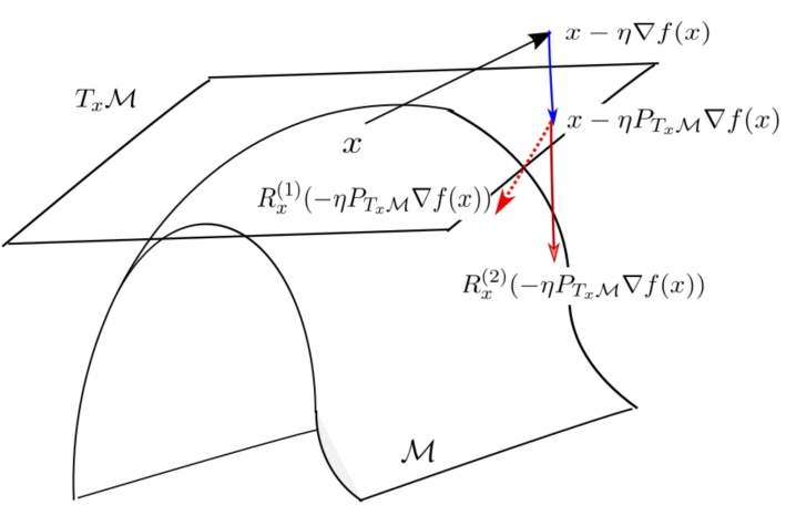
Define a retraction that maps the tangent space back to the manifold, i.e. , where needs to satisfy the conditions in [37, Definition 2.2]. In particular, , as , and needs to be smooth. Then the update of the gradient descent algorithm is defined by
(2) where is the step size.
Note that the definition of retraction is not unique. In Figure 1, we visualize the gradient descent method on the manifold with two different kinds of retractions (orthographic and projective). We will discuss the details of those two retractions in Section 2.2.
2.2 The geometry of the manifold of low-rank matrices
Now we apply the above gradient descent algorithm to the manifold of the low-rank matrices. Let be the manifold of all matrices with rank and denote a specific matrix . The tangent space and the retraction of the manifold of the low-rank matrices have been well-studied [2]. The tangent space can be defined by where and according to [2]. The explicit formula for the projection is given in [2, (9)]. Assume . Denote the SVD decomposition of as , then
| (3) |
The formula (13) can be verified as follows. Note that can be equivalently defined by for any matrices , , such that and , thus . Furthermore, let be the Frobenius inner product of two matrices, then
and similarly . As a result, for all and , which verifies the formula (13).
There are various ways of defining retractions for the manifold of low-rank matrices, and we refer the reader to [2] for more details. In this work, we consider only two types of retractions. One is called the projective retraction [34, 37], defined as the nearest low-rank matrix to in terms of Frobenius norm:
| (4) |
for and the solution is given by , where are the ordered singular values and vectors of respectively. In order to further improve computation efficiency, we also consider the orthographic retraction [2]. Denoted by , it is the nearest low-rank matrix to such that
| (5) |
[2, Section 3.2] gives an explicit formula for the orthographic retraction,
| (6) |
Later we will show that the solution has a simple explicit formula and there is no need to calculate singular value decomposition as the projective retraction.
3 Proposed algorithms
To recover , we solve the following optimization problem:
| (7) |
where is a hard thresholding procedure defined by
| (8) |
Here represents the -th row of , and represents the -th column of . and represent the -th percentile of the absolute values of the entries of the -th row and the -th column respectively. In other words, those elements that are simultaneously among the largest -fraction entries in terms of absolute values in the corresponding row and column of are removed. The threshold is set by users. If some entries of or have the elements with identical absolute values, the ties can be broken down arbitrarily.
By applying (2), the iterative algorithm for solving (7) can be written by
| (9) |
In the following we provide the explicit formulas for the gradient , projection and retraction operations in (9).
To find , we define the operator :
Then if the absolute values of all entries of are different, the sparsity pattern does not change under a small perturbation, i.e., Then by definition of ,
where represents the Hadamard product, i.e., the elementwise product between matrices. This implies
| (10) |
Therefore, the gradient descent algorithm with projective retraction can be written as follows, with defined later in (13):
| (11) |
and for orthographic retraction,
| (12) |
Now we get the explicit formula for the projection . Write . Given the SVD decomposition , we have the projection
| (13) |
To compute the projective retraction , where , we get the singular value decomposition . The projective retraction is
where is a matrix consists of the first columns of ; is a matrix consists of the first columns of ; is the upper left submatrix of , and . The orthographic retraction is
| (14) |
We remark that for the formula (12) can be further simplified. Note that
| (15) |
and similarly,
Let and , by (10) and (3), we have
and
So the update formula (12) can be simplified to
| (16) |
In addition, it can be shown that and in (14) and (16) can be replaced by and for any nonsingular matrices . That is, and in (14) and (16) can be replaced by any matrices and that have the same column spaces as and respectively.
The complete procedures of the implementation are summarized in Algorithm 1 and Algorithm 2. It can be shown that both algorithms have a complexity of per iteration, but empirically the gradient descent with the orthographic retraction is faster since it does not need to compute the singular value decomposition of in each iteration.
Input: Observation ; Rank ; Thresholding value ; Step size .
Initialization: Set ; Initialize using the rank- approximation to .
Loop: Iterate Steps 1–3 until convergence:
- 1.
-
2.
Let be the rank approximation of or .
-
3.
.
Output: Estimation of the low-rank matrix, given by .
Input: Observation ; Rank ; Thresholding value ; Step size .
Initialization: Set ; Initialize using the rank- approximation to .
Loop: Iterate Steps 1–3 until convergence:
- 1.
-
2.
Let consists of any independent columns of , and consists of any independent rows of , and
-
3.
.
Output: Estimation of the low-rank matrix, given by .
3.1 Partial Observations
The proposed algorithm can be generalized to the setting of partial observations, i.e., in addition to gross corruptions, the data matrix has a large number of missing values. We assume that each entry of is observed with probability , and denote the set of all observed entries by .
For this case, our optimization problem is given by
where is defined by
| (17) |
Here and represent the -th percentile of the absolute values of the observed entries of the -th row and the -th column respectively.
4 Theoretical analysis
In this section, we analyze the theoretical properties of our gradient descent algorithms on the manifold and compare them with previous algorithms. To avoid identifiability issues, we need to make sure that can not be both low-rank and sparse. Specifically, we make the following standard assumptions on and :
-
1.
Each row of contains at most nonzero entries and each column of contains at most nonzero entries. In other words, for , assume where
(18) -
2.
The low-rank matrix is not near-sparse. To achieve this, we require that must be -coherent. Given the singular value decomposition (SVD) , where and , we assume
(19) where the norm is defined by and .
With assumptions (18) and (19), we have the following theoretical results regarding the convergence rate, initialization and stability of Algorithm 1 and Algorithm 2:
Theorem 1 (Convergence rate, partially-observed case).
The gradient descent algorithms have a linear convergence rate. Suppose that , where is the -th largest singular value of , , and , then there exists such that for all ,
Remark 1.
In particular, if there exists and such that if , and , then one can choose .
Theorem 2 (Convergence rate, partially-observed case).
There exists such that for , if , then with probability , for all ,
for
Remark 2.
In particular, if there exists such that when , , and , then we can choose , thus when ,
Since both statements require proper initializations, the question arises as to how to choose proper initializations. The work by [40] shows that if the rank- approximation to is used as the initialization , then such initialization has the upper bound according to the proofs of [40, Theorems 1 and 3] (we borrow this estimation along with the fact that ).
Theorem 3 (Initialization, partially-observed case).
If and we initialize using the rank- approximation to , then
Theorem 4 (Initialization, partially-observed case).
There exists and such that if , and , and we initialize using the rank- approximation to , then
with probability at least , where is the largest singular value of
The combination of Theorem 1 and 3 implies that, for the partially-observed setting, the tolerance of the proposed algorithms to corruption is at most , where is the conditional number of . The combination of Theorem 2 and 4 implies that, for the partially-observed setting, the proposed algorithm allows the corruption level .
We also study the stability of the algorithm for the partially-observed case.
Theorem 5 (Stability, partially-observed case).
Theorem 5 shows that when the observation is contaminated with a random Gaussian noise, if is properly initialized such that , Algorithms 1 and 2 can converge to a neighborhood of given by
with high probability.
4.1 Comparison with previous works
Theorems 1 and 2 are in parallel with the analysis in [40], which is natural since the objective function (7) is equivalent to the one in [40]. Our methods use the gradient descent on the manifold of low-rank matrices, while the methods in [40] use the Burer-Monteiro decomposition. In the following we compare the results of both works from four aspects:
-
1.
Accuracy of initialization. What is the largest value that the algorithm can tolerate, such that for any initialization satisfying , the algorithm is guaranteed to converge to ?
-
2.
Convergence rate. What is the smallest number of iteration steps such that the algorithm reaches a given convergence criterion , i.e. ?
-
3.
Corruption level (perfect initialization). Suppose that the initialization is in a sufficiently small neighborhood of (i.e. there exists a very small such that satisfies ), what is the maximum corruption level that can be tolerated in the convergence analysis?
- 4.
These comparisons are summarized in Table 1. We can see that in the full observed setting, our results remove or reduce the dependence on the conditional number , while keeping other values unchanged. In the partially-observed setting our results still have the advantage of less dependence on , but sometimes require an additional dependence on . The simulation results discussed in the next section also verify that when is large our algorithms have better performance, while that the slowing effect of in the partially-observed setting is not significant.
The results in [28] and [12] are less comparable since these algorithms are based on the alternative projection instead of the gradient descent. In fact, in the partially-observed case, [28] achieves exact recovery when . Compared with obtained from combining Theorem 1 and 3, [28] removes the dependence on and reduces the dependence on , but requires a stronger dependence on . In addition, the algorithm in [28] has a complexity of . It is slightly more expensive than , which is the complexity of our algorithms and the algorithms in [40].
| Criterion | 1 | 2 | 3 | 4 |
|---|---|---|---|---|
| Proposed method (full) | ||||
| [40] (full) | ||||
| Proposed method (partial) | ||||
| [40] (partial) |

5 Simulations
In this section, we compare the computational performances of our method and the method in [40]. In simulations, we let , , and is generated from , where and are random orthogonal matrices of size and . We consider the following two settings:
-
•
Setting 1. (the condition number is thus 1), is obtained by replacing elements in each column of by a random number from Gaussian distribution , and let .
-
•
Setting 2. (the condition number is thus 10), , and let .
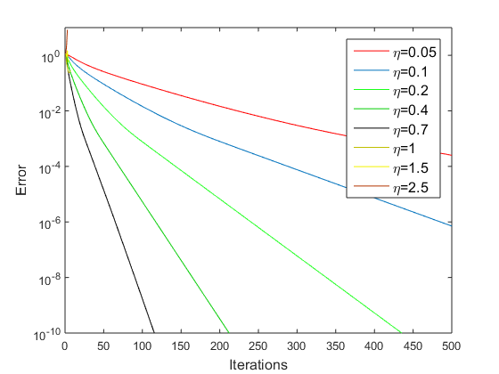
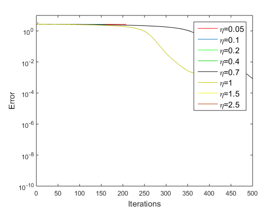
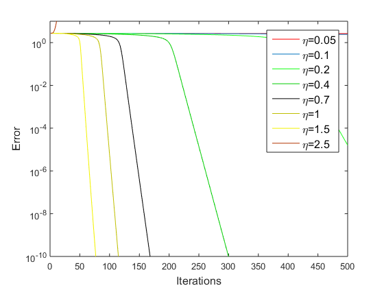
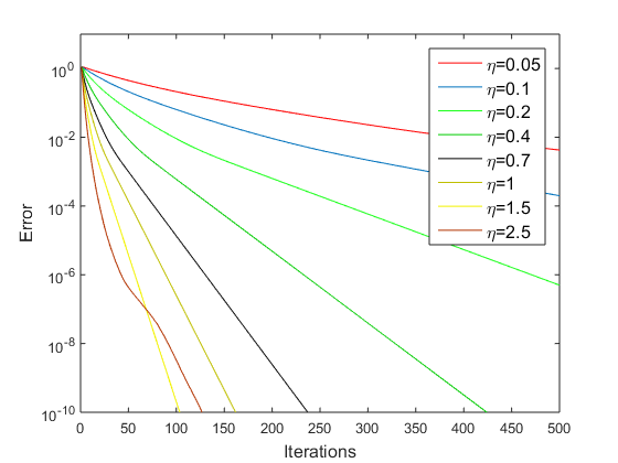
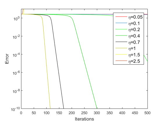
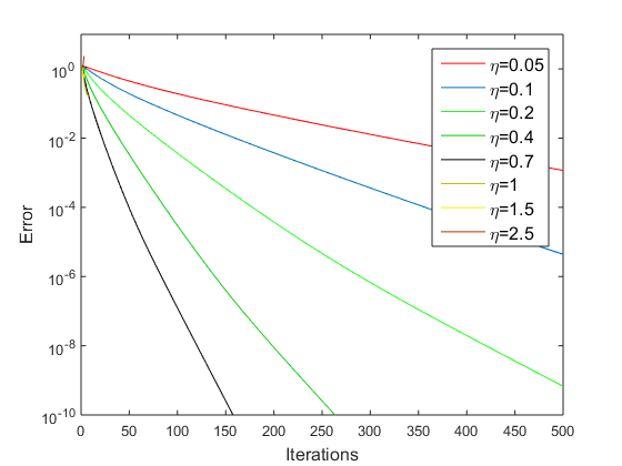
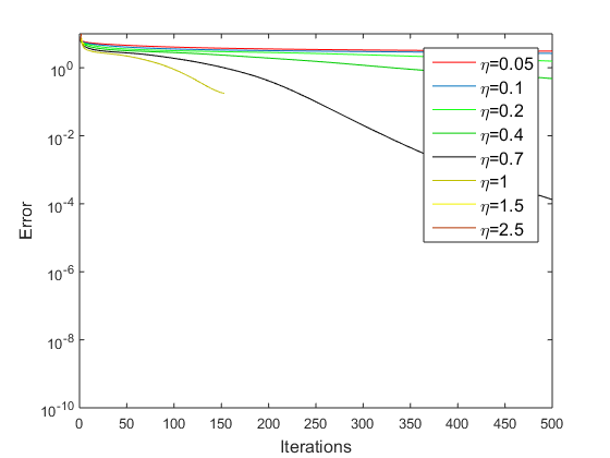
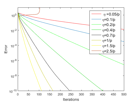
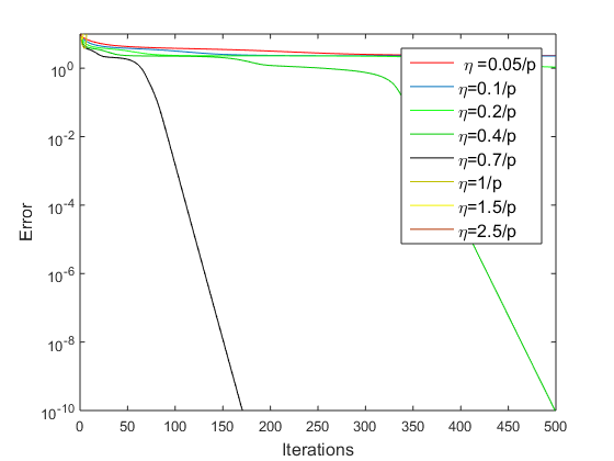
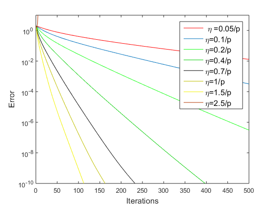
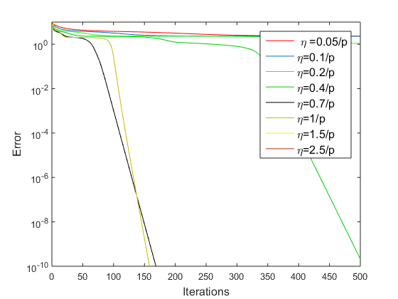
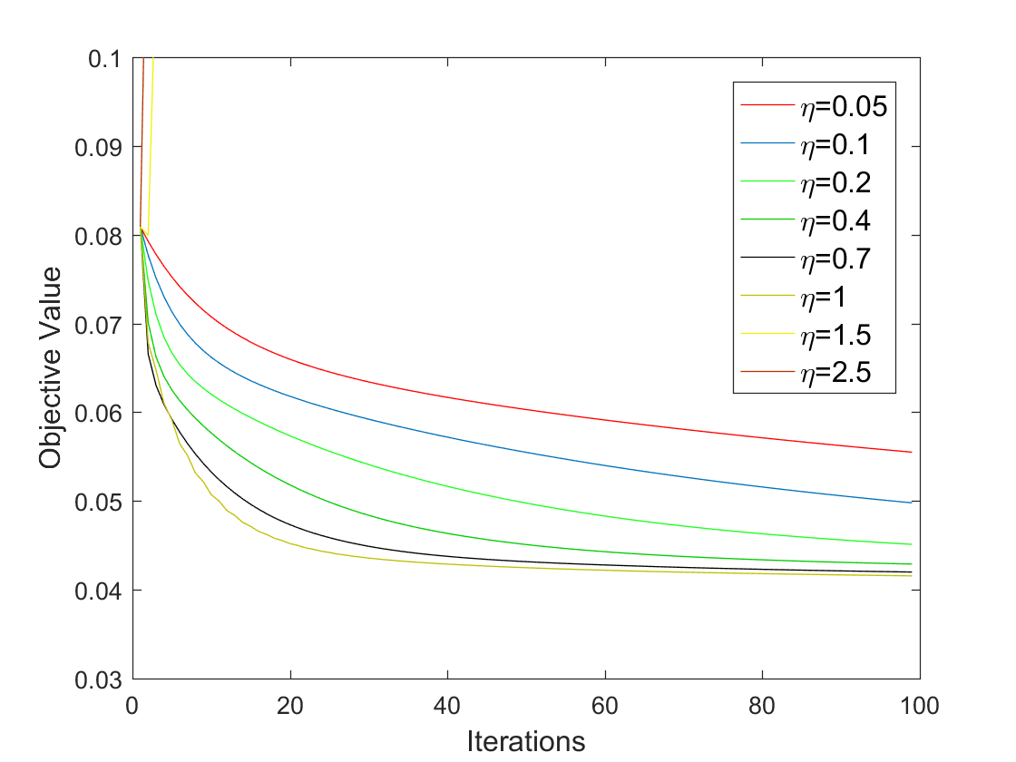
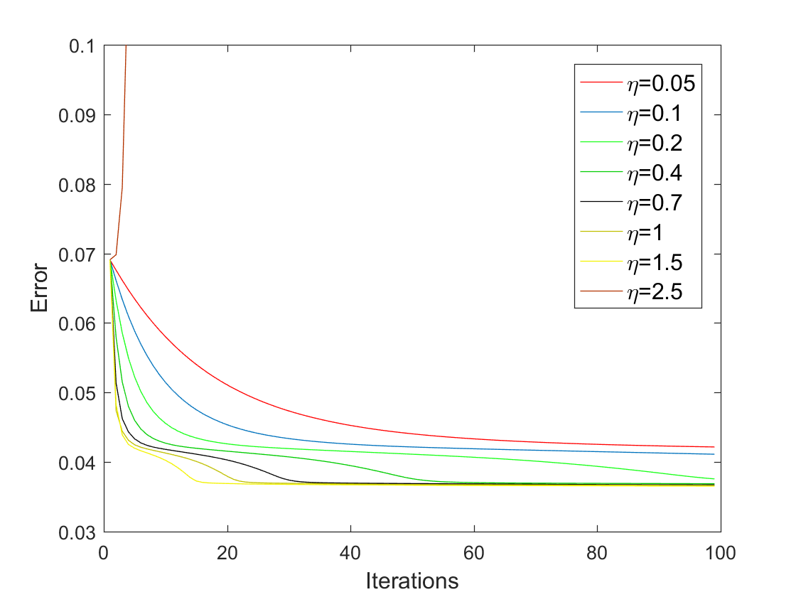
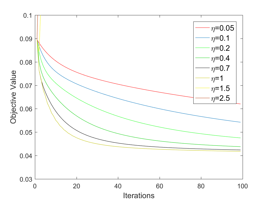
The performance of the algorithms with various choices of step sizes are recorded in Figure 2 and 3, where the error is measured by the Frobenius norm of the difference to the underlying low-rank matrix, i.e. for all . For all cases of the simulation results, the algorithms usually converge faster with larger step sizes, but will diverge once reach a certain threshold. Therefore in all simulations we test a wide range of step sizes , so that the best step sizes are included. For example, for the upper-left figure in Figure 2 and 3, the algorithm converges when is between and , and diverges when , and is the best step size in terms of convergence rate. For the partially-observed setting, we use the step sizes with a factor as it works well empirically.
Figure 2 and 3 show that our algorithms converge linearly, and faster than the algorithm in [40] when the step sizes are well-chosen. The performance our algorithms is also less sensitive to the choice of step sizes. For both Setting 1 and 2, both partially-observed cases and partially-observed cases, our algorithms converge within iterations for a wide range of . The advantage of our algorithms are more obvious when the conditional number is large. In particular, the right columns of Figure 2 and 3 visualize the cases for Setting 2 when the conditional number of is . Under these cases, the advantage of our algorithms in convergence rate becomes more obvious. This verifies the analysis in Section 4.1 that our algorithms remove or reduce the dependence of the convergence on the conditional number . In addition, we observed that the performance of our algorithms in the partially-observed case is not significantly affected by the presence of the additional dependence on the observation probability .
In addition, the simulations shows that the projective retraction and the orthographic retraction usually has no significant difference in terms of performance. In fact, their performance are almost identical except in Figure 2, when for partially-observed case and in Figure 3, when for partially-observed case, both under Setting 2. Since it is less computationally extensive to calculate the orthographic retraction (the projective retraction requires an additional singular value decomposition in each iteration), we recommend to use Algorithm 2, especially when the computational complexity is concerned.
We test Algorithm 2 in a real data application for video background subtraction. We adopt the public data set Shoppingmall studied in [40],111The data set is originally from http://perception.i2r.a-star.edu.sg/bk_model/bk_index.html, and is available at https://sciences.ucf.edu/math/tengz/. A few frames are visualized in the first column of Figure 4. There are 1000 frames in this video sequence, represented by a matrix of size , where each column corresponds to a frame of the video and each row corresponds to a pixel of the video. We apply Algorithm 2 with and , for the partially-observed case, the step size . We stop the algorithm after 100 iterations. Figure 4 shows that our algorithms obtain desirable low-rank approximations within iterations. In Figure 5, we also compare Algorithm 2 and the method in [40] with respect to the convergence of the objective function value, and we expect that a smaller objective function implies a better low-rank approximation. It turns out that our algorithm can consistently obtain smaller objective value within 100 iterations under both fully-observed and partially-observed settings.


6 Conclusion
In this paper we propose two robust PCA algorithms (one for projective retraction and one for orthographic retraction) based on the gradient descent algorithm on the manifold of low-rank matrices. Theoretically, compared with the gradient descent algorithm with Burer-Monteiro decomposition, our approach has a faster convergence rate, better tolerance of the initialization accuracy and corruption level. The approach removes or reduces the dependence of the algorithms on the conditional number of the underlying low-rank matrix. Numerically, the proposed algorithms performance is less sensitive to the choice of step sizes. We also find that under the partially-observed setting, the performance of the proposed algorithm is not significantly affected by the presence of the additional dependence on the observation probability. Considering the popularity of the Burer-Monteiro decomposition, it is an interesting future direction to apply manifold optimization to other low-rank matrix estimation problems.
Appendix for “Robust Principal Component Analysis by Manifold Optimization”
A. Proof of Theorem 1
In this proof, we will investigate , where
It is sufficient to prove that when with satisfying the conditions in Theorem 1, then
| (20) |
To prove (20), we first introduce three auxiliary lemmas.
Lemma 1.
-
(a) Let , then
(21) -
(b) For the noisy setting where , and , we have
(22) where .
Lemma 2.
If and , then
| (23) | ||||
| (24) |
Lemma 3.
For , then
To prove (20), first we note that
| (25) |
Lemma 2 and the assumptions , imply
| (26) |
Combining it with the estimation of in Lemma 1, we have
| (27) |
When ths RHS of (27) is positive (i.e., when ), (27) implies and
| (28) |
In addition,
| (29) |
and Lemma 3 give
| (30) |
Therefore, Theorem 1 is proved when , and is chosen such that
B. Proof of Theorem 2
This proof borrows two lemmas from [40, lemma 9, 10] as follows.
Lemma 4.
[40, Lemma 9] There exists such that for all , if , then with probability at least , for any
Lemma 5.
[40, Lemma 10] If , the with probability at least , the number of entries in per row is in the interval , and the number of entries in per column is in .
Then we introduce the following lemma parallel to Lemma 1:
The proof of Theorem 2 is parallel to the proof of Theorem 1, with defined slightly differently by
Defining by
Then . Following a similar analysis as (25),
| (32) |
and combining it with the estimation of in Lemma 6, the RHS of (32) is larger than
| (33) |
In addition, Lemma 4 implies
and combining it with Lemma 3,
Combining it with (33) and Lemma 2, we have
and Theorem 2 is proved.
C. Proof of Theorem 5
The proof of the noisy case also follows similarly from the proofs of Theorem 1 and 2. Note that
and define , then following the proof of Theorem 1 and applying Lemma 1 (b), we have
In addition, (30) gives
Combining it with the estimation of , , and in Lemma 7 and the fact that (which follows from Lemma 2), the Theorem is proved.
Lemma 7.
If is elementwisely i.i.d. sampled from , then
(a) with probability , , and , and as a result, .
(b) There exists such that as , the probability that
| (34) |
holds for all converges to 1.
D. Proof of Lemmas
Proof of Lemma 1(a)
Proof.
By the definition of , is a sparse matrix. Denote the locations of the nonzero entries by , and divide it into two sets as follows:
and
For , . As a result, .In addition, by definition, each row or column has at most percentage of points in .
For , . Therefore, for each row or column, at most percentage of points lie in . Since , and
we have
Applying the estimations above, and repeatedly use the fact that , we have
| (35) |
In another aspect, Lemma 2 implies
| (36) |
In addition, since there exists such that , and for each row or column, at most percentage of points lie in ,
| (37) |
Similarly,
| (38) |
Proof of Lemma 1(b)
Proof.
Let , then applying the fact that for any ,
we have
where the last inequality follows from the proof of part (a) and the definition of .∎
Proof of Lemma 6
Proof of Lemma 2
Proof.
Let the SVD decomposition of be , and be orthogonal matrices of sizes and such that and (here represents the spanned spanned by the columns of ), and
Since , we have
Since all singular values of are larger than , if the singular value decomposition of is given by
then the . Applying
and the fact that for a square, diagonal matrix , , we have
| (39) |
Proof of Lemma 3
Proof of Lemma 7
Proof.
In the proof WLOG we assume and the generic cases can be proved similarly.
(a) It follows from the estimation of distribution of the maximum of i.i.d. Gaussian variables :
where the first inequality applies the estimation of the cumulative distribution function of the Gaussian distribution [24, pg 8].
Combining this estimation for each column of and applying the union bound, the second inequality in part (a) holds with probability . Similarly, the first inequality in part (a) holds with the same probability.
(b) First, we parameterize by . Then we claim that, for any and such that , there exists depending on such that
| (40) |
To prove (40), apply (24) and obtain
| (41) |
Since , and using Davis-Kahan theorem [14] and the assumption , there exists , depending on such that
so there exists depending on such that
| (42) | ||||
Second, based on (40), we will apply an -net covering argument to finish the proof that combines probabilistic estimation for each and a union bound (-net covering argument is a standard argument in probabilistic estimation [38]). Use the estimation of the cumulative distribution function of the Gaussian distribution [24, pg 8], for any ,
For any such that , applying (40),
Using union bound, there is an -net of the set with at most points. Therefore, for all such that ,
| (43) |
Let and , then when (which holds with high probability as goes to infinity), then using we have , and when ,
| (44) |
where the last inequality applies the assumption . Combining (43) and (44) and recall that , we have that for all such that ,
| (45) |
Let with , then
| (46) |
where the last inequality uses when . Clearly, the RHS goes to as .
References
- [1] P. Absil, R. Mahony, and R. Sepulchre. Optimization Algorithms on Matrix Manifolds. Princeton University Press, 2009.
- [2] P.-A. Absil and I. V. Oseledets. Low-rank retractions: a survey and new results. Computational Optimization and Applications, 62(1):5–29, 2015.
- [3] A. S. Bandeira, N. Boumal, and V. Voroninski. On the low-rank approach for semidefinite programs arising in synchronization and community detection. In V. Feldman, A. Rakhlin, and O. Shamir, editors, 29th Annual Conference on Learning Theory, volume 49 of Proceedings of Machine Learning Research, pages 361–382, Columbia University, New York, New York, USA, 23–26 Jun 2016. PMLR.
- [4] R. Basri and D. Jacobs. Lambertian reflectance and linear subspaces. IEEE Transactions on Pattern Analysis and Machine Intelligence, 25(2):218–233, February 2003.
- [5] S. Bhojanapalli, P. Jain, and S. Sanghavi. Tighter low-rank approximation via sampling the leveraged element. In Proceedings of the Twenty-sixth Annual ACM-SIAM Symposium on Discrete Algorithms, SODA ’15, pages 902–920, Philadelphia, PA, USA, 2015. Society for Industrial and Applied Mathematics.
- [6] N. Boumal. Nonconvex phase synchronization. SIAM Journal on Optimization, 26(4):2355–2377, 2016.
- [7] S. Burer and R. D. Monteiro. A nonlinear programming algorithm for solving semidefinite programs via low-rank factorization. Mathematical Programming, 95(2):329–357, 2003.
- [8] S. Burer and R. D. Monteiro. Local minima and convergence in low-rank semidefinite programming. Mathematical Programming, 103(3):427–444, 2005.
- [9] E. J. Candès, X. Li, Y. Ma, and J. Wright. Robust principal component analysis? J. ACM, 58(3):11:1–11:37, June 2011.
- [10] V. Chandrasekaran, S. Sanghavi, P. A. Parrilo, and A. S. Willsky. Rank-sparsity incoherence for matrix decomposition. SIAM Journal on Optimization, 21(2):572–596, 2011.
- [11] Y. Chen and M. J. Wainwright. Fast low-rank estimation by projected gradient descent: General statistical and algorithmic guarantees. CoRR, abs/1509.03025, 2015.
- [12] Y. Cherapanamjeri, K. Gupta, and P. Jain. Nearly-optimal robust matrix completion. CoRR, abs/1606.07315, 2016.
- [13] K. L. Clarkson and D. P. Woodruff. Low rank approximation and regression in input sparsity time. In Proceedings of the Forty-fifth Annual ACM Symposium on Theory of Computing, STOC ’13, pages 81–90, New York, NY, USA, 2013. ACM.
- [14] C. Davis and W. M. Kahan. The rotation of eigenvectors by a perturbation. iii. SIAM Journal on Numerical Analysis, 7(1):1–46, 1970.
- [15] C. De Sa, K. Olukotun, and C. Ré. Global convergence of stochastic gradient descent for some non-convex matrix problems. In Proceedings of the 32Nd International Conference on International Conference on Machine Learning - Volume 37, ICML’15, pages 2332–2341. JMLR.org, 2015.
- [16] S. Deerwester, S. T. Dumais, G. W. Furnas, T. K. Landauer, and R. Harshman. Indexing by latent semantic analysis. Journal of the American Society for Information Science, 41(6):391–407, 1990.
- [17] R. Epstein, P. Hallinan, and A. Yuille. eigenimages suffice: An empirical investigation of low-dimensional lighting models. In IEEE Workshop on Physics-based Modeling in Computer Vision, pages 108–116, June 1995.
- [18] A. Frieze, R. Kannan, and S. Vempala. Fast monte-carlo algorithms for finding low-rank approximations. J. ACM, 51(6):1025–1041, Nov. 2004.
- [19] Q. Gu, Z. Wang, and H. Liu. Low-rank and sparse structure pursuit via alternating minimization. In A. Gretton and C. C. Robert, editors, AISTATS, volume 51 of JMLR Workshop and Conference Proceedings, pages 600–609. JMLR.org, 2016.
- [20] J. Ho, M. Yang, J. Lim, K. Lee, and D. Kriegman. Clustering appearances of objects under varying illumination conditions. In Proceedings of International Conference on Computer Vision and Pattern Recognition, volume 1, pages 11–18, 2003.
- [21] D. Hsu, S. M. Kakade, and T. Zhang. Robust matrix decomposition with sparse corruptions. IEEE Transactions on Information Theory, 57(11):7221–7234, Nov 2011.
- [22] P. Jain, P. Netrapalli, and S. Sanghavi. Low-rank matrix completion using alternating minimization. In Proceedings of the Forty-fifth Annual ACM Symposium on Theory of Computing, STOC ’13, pages 665–674, New York, NY, USA, 2013. ACM.
- [23] A. Kyrillidis and V. Cevher. Matrix alps: Accelerated low rank and sparse matrix reconstruction. In 2012 IEEE Statistical Signal Processing Workshop (SSP), pages 185–188, Aug 2012.
- [24] M. Ledoux and M. Talagrand. Probability in Banach Spaces: Isoperimetry and Processes. A Series of Modern Surveys in Mathematics Series. Springer, 1991.
- [25] L. Li, W. Huang, I. Gu, and Q. Tian. Statistical modeling of complex backgrounds for foreground object detection. Image Processing, IEEE Transactions on, 13(11):1459 –1472, nov. 2004.
- [26] X. Li and J. Haupt. Identifying outliers in large matrices via randomized adaptive compressive sampling. IEEE Transactions on Signal Processing, 63(7):1792–1807, April 2015.
- [27] L. W. Mackey, M. I. Jordan, and A. Talwalkar. Divide-and-conquer matrix factorization. In J. Shawe-Taylor, R. S. Zemel, P. L. Bartlett, F. Pereira, and K. Q. Weinberger, editors, Advances in Neural Information Processing Systems 24, pages 1134–1142. Curran Associates, Inc., 2011.
- [28] P. Netrapalli, N. U N, S. Sanghavi, A. Anandkumar, and P. Jain. Non-convex robust pca. In Z. Ghahramani, M. Welling, C. Cortes, N. D. Lawrence, and K. Q. Weinberger, editors, Advances in Neural Information Processing Systems 27, pages 1107–1115. Curran Associates, Inc., 2014.
- [29] D. Park, A. Kyrillidis, S. Bhojanapalli, C. Caramanis, and S. Sanghavi. Provable Burer-Monteiro factorization for a class of norm-constrained matrix problems. jun 2016.
- [30] D. Park, A. Kyrillidis, C. Carmanis, and S. Sanghavi. Non-square matrix sensing without spurious local minima via the Burer-Monteiro approach. In A. Singh and J. Zhu, editors, Proceedings of the 20th International Conference on Artificial Intelligence and Statistics, volume 54 of Proceedings of Machine Learning Research, pages 65–74, Fort Lauderdale, FL, USA, 20–22 Apr 2017. PMLR.
- [31] A. L. Price, N. J. Patterson, R. M. Plenge, M. E. Weinblatt, N. A. Shadick, and D. Reich. Principal components analysis corrects for stratification in genome-wide association studies. Nature genetics, 38(8):904–909, aug 2006.
- [32] M. Rahmani and G. K. Atia. High dimensional low rank plus sparse matrix decomposition. IEEE Transactions on Signal Processing, 65(8):2004–2019, April 2017.
- [33] A. Ruhe. Numerical Computation of Principal Components when Several Observations are Missing. Univ., 1974.
- [34] U. Shalit, D. Weinshall, and G. Chechik. Online learning in the embedded manifold of low-rank matrices. J. Mach. Learn. Res., 13(1):429–458, Feb. 2012.
- [35] J. Sun, Q. Qu, and J. Wright. Complete dictionary recovery over the sphere i: Overview and the geometric picture. IEEE Transactions on Information Theory, 63(2):853–884, Feb 2017.
- [36] S. Tu, R. Boczar, M. Simchowitz, M. Soltanolkotabi, and B. Recht. Low-rank solutions of linear matrix equations via procrustes flow. In Proceedings of the 33nd International Conference on Machine Learning, ICML 2016, New York City, NY, USA, June 19-24, 2016, pages 964–973, 2016.
- [37] B. Vandereycken. Low-rank matrix completion by riemannian optimization. SIAM Journal on Optimization, 23(2):1214–1236, 2013.
- [38] R. Vershynin. Introduction to the non-asymptotic analysis of random matrices. In Y. C. Eldar and G. Kutyniok, editors, Compressed Sensing: Theory and Practice, pages 210–268. Cambridge University Press, 2012.
- [39] L. Wang, X. Zhang, and Q. Gu. A Unified Computational and Statistical Framework for Nonconvex Low-rank Matrix Estimation. In A. Singh and J. Zhu, editors, Proceedings of the 20th International Conference on Artificial Intelligence and Statistics, volume 54 of Proceedings of Machine Learning Research, pages 981–990, Fort Lauderdale, FL, USA, 20–22 Apr 2017. PMLR.
- [40] X. Yi, D. Park, Y. Chen, and C. Caramanis. Fast algorithms for robust PCA via gradient descent. In Advances in Neural Information Processing Systems 29: Annual Conference on Neural Information Processing Systems 2016, December 5-10, 2016, Barcelona, Spain, pages 4152–4160, 2016.