Optical spectroscopy of a microsized Rb vapour sample in magnetic fields up to 58 tesla

Abstract

We use a magnetometer probe based on the Zeeman shift of the rubidium resonant optical transition to explore the atomic magnetic response for a wide range of field values. We record optical spectra for fields from few tesla up to 60 tesla, the limit of the coil producing the magnetic field. The atomic absorption is detected by the fluorescence emissions from a very small region with a submillimiter size. We investigate a wide range of magnetic interactions from the hyperfine Paschen-Back regime to the fine one, and the transitions between them. The magnetic field measurement is based on the rubidium absorption itself. The rubidium spectroscopic constants were previously measured with high precision, except the excited state Landé $g$-factor that we derive from the position of the absorption lines in the transition to the fine Paschen-Back regime. Our spectroscopic investigation, even if limited by the Doppler broadening of the absorption lines, measures the field with a 20 ppm uncertainty at the explored high magnetic fields. Its accuracy is limited to 75 ppm by the excited state Landé $g$-factor determination

I Introduction

The present large effort of the quantum control research is the miniaturization and manipulation from the micron scale down to the single atom. This objective is important for a complete quantum control and also for the development of new tools for applications, as geophysics, biophysics, brain imaging, and more. Recently a large attention was concentrated on the magnetic response and the measurement of weak magnetic fields with a high spatial resolution. Technologies capable of micron-scale magnetic microscopy include SQUID devices, scanning Hall probe microscopes, magnetic force microscopes, magneto-optical imaging techniques. Magnetic fields may also be measured by detecting the Zeeman splitting for warm and ultracold atoms Kominis et al. (2003); Vengalattore et al. (2007), nuclei in a ferromagnetic material Mamin et al. (2007), or impurities in diamond (NV-centers) Taylor et al. (2008); Pham et al. (2011); Rondin et al. (2014).
The same large attention was not reserved to the measurement of high magnetic fields, whose application range is steadily growing. Nowadays accurate measurements of high magnetic fields are performed via the Zeeman splitting in nuclear magnetic resonance of hydrogen in water. This technique based on radiofrequency/microwave frequency absorption, is applied mainly to continuous magnetic fields, with an uncertainty better than 1 ppm over a volume of a few mm³. As well know from optical pumping, the detection of higher energy photons, i.e. as optical ones, greatly increases the measurement efficiency Budker and Kimball (2013). In presence of an applied magnetic field, atomic optical transitions experience a Zeeman frequency shift, and today laser frequency are measured with very high precision. The measure of a Zeeman shift is routinely applied to magnetic field in plasmas produced by an exploding wire Garn et al. (1966); Hori et al. (1982); Gomez et al. (2014); Banasek et al. (2016), where the high sample temperature limits the precision.
We have developed an optical spectroscopy magnetic field probe based on the Zeeman splitting in a rubidium atomic sample with a volume of 0.11 mm${}^{3}~{}$George et al. (2017). The present investigation of atomic spectroscopy at high magnetic fields is based on that probe. Our experiment operates with pulsed magnetic fields having rise and fall times around 100 milliseconds. Even if the detection is based on Doppler limited absorption spectroscopy, at the explored fields around 60 T the reached 20 ppm uncertainty allows us to perform high resolution optical spectroscopy.
We report a precise study of the Zeeman effect for the rubidium $5^{2}S_{1/2}\to 5^{2}P_{3/2}$ resonance line in magnetic field regimes not well explored. Our results demonstrate that under a high resolution investigation the classification of the regimes as hyperfine or fine Paschen-Back ones Kopfermann (1958) represents a rough schematization for the atomic response. The data evidence that the hyperfine Paschen-Back regime is fully reached at magnetic fields larger than the standard comparison between electronic Zeeman energy and hyperfine structure splitting. On the other side, a theoretical description based on the fine Paschen-Back approach is required to interpret data collected at magnetic fields lower than the standard comparison between electronic Zeeman energy and fine structure splitting.
As original feature, our measurement does not rely on the presence of an independent magnetometer, and the magnetic field value is derived directly from the measured rubidium optical absorption. The determination is based on the existence of an optical Zeeman shift characterized by a field linear dependence, at all magnetic field values. That measurement combined with the magnetic field temporal evolution detected by a pick-up coil provides the absolute scale for the whole explored magnetic range. All atomic constants determining the rubidium absorption frequencies are well known from previous investigations, except for the Landé $g$-factor of the excited 5P state. Within the target of using the rubidium optical transitions for an atomic magnetometer, its precise value is required. We have derived the excited state Landé $g$-factor by exploring the magnetic field dependence of different optical transitions. The ratio of the associated resonance fields, independent on the magnetic field absolute calibration, provides this atomic constant with high precision. The accuracy of the rubidium based magnetometry is limited to 75 ppm by our $g$-factor uncertainty.
Section II describes the response to high magnetic fields, presenting eigenstates, eigenenergies and optical transitions starting from the hyperfine Paschen-Back approximation. The diamagnetic contribution to the rubidium energy levels of interest is discussed. We introduce the optical transition line used for the magnetic field calibration. The Section is completed by a brief discussion on the atomic magnetic data required for our analyses. Section III describes the experimental set-up, with the absorption detection based on the fluorescence detection in order to decrease the observation volume. Section IV reports examples of recorded spectra, their analysis and the role played by the nuclear interaction. This Section includes also the analysis of the ratio of the high/low magnetic resonant fields for the $\sigma^{+}$ lines. The modification of the full fine structure multiplet is required for the data interpretation leading us to the Landé $g$-factor determination. A final Section concludes our work.

II Rubidium in high magnetic field

II.1 Paramagnetism

For an alkali atom, the magnetic interaction of the valence electron is described through several quantum numbers, for the nucleus the $(I,m_{I})$ spin components, for the electron the $(L,m_{L})$ orbital angular momentum, the $(S,m_{S})$ spin, the vector composition of $\mathbf{L}$ and $\mathbf{S}$ with $(J,m_{J})$ components, and finally the vector composition of $\mathbf{J}$ and $\mathbf{I}$ with components $(F,m_{F})$. As in textbooks Kopfermann (1958), at very low magnetic fields, where the electron-nucleus hyperfine interaction is larger than the electronic Zeeman interaction, $(F,m_{F})$ are the correct quantum numbers. Increasing the magnetic field the hyperfine Paschen-Back regime is reached when the role between hyperfine interaction and electronic Zeeman energy is reversed Kopfermann (1958). There $(J,m_{J})$ are the good quantum numbers. Because for rubidium the $5^{2}S_{1/2}$ ground state hyperfine interaction is around fifty times larger than the $5^{2}P_{3/2}$ excited state one, the hyperfine Paschen-Back regime should be reached when the electron Zeeman energy is roughly equal to the the ground state interaction, around 0.5 T for ⁸⁷Rb. While for the ground state $(J,m_{J})$ remain good quantum numbers for all higher magnetic fields, for the excited state the fine structure splitting between $5^{2}P_{1/2}$ and $5^{2}P_{3/2}$ states must be compared to the electronic Zeeman splitting. For rubidium the fine Paschen-Back regime is reached at fields around 500 T. There $(L=1,m_{L})$ and $(S=1/2,m_{S})$ are the quantum numbers, combined with the nuclear spin. This regime was never explored in rubidium, while owing to the smaller fine structure splitting it was explored for sodium in experiments with exploding wires Garn et al. (1966); Hori et al. (1982); Gomez et al. (2014); Banasek et al. (2016).
At high fields the diamagnetism contribution to the magnetic interaction should be included in the analysis, as in Sec IIC. However our experiment demonstrates this contribution negligible for fields up to 60 T. For completeness refs. Lipson et al. ; Fortson explored for the rubidium ground state a Zeeman energy term induced by the magnetic dipole hyperfine interaction, through a coupling of higher electronic levels into the ground state, term quadratic in $m_{I}$ and equivalent to a modification of the nuclear $g$-factor. This shift is only few Hz at our largest explored field.
Following the above classification, the 1-60 T explored magnetic field range corresponds to the hyperfine Paschen-Back regime. Thus the rubidium ground state is specified by $(J_{g}=1/2,m_{Jg})$, combined with $(I,m_{I})$. The two stable isotopes, ⁸⁵Rb and ⁸⁷Rb, have nuclear spin, $I=5/2$ and $I=3/2$, respectively, characterized by the nuclear Landé $g$-factor $g_{I}$, assumed negative as in Arimondo et al. (1977). For the alkali ground state, the eigenenergies are given by the Breit-Rabi formula Kopfermann (1958); Foot (2012), including the electronic and nuclear Zeeman energies and the $A_{g}$ dipolar hyperfine coupling.
For the excited state, no analytical formula exist for the eigenenergies, to be derived by diagonalizing numerically the Hamiltonian. For the hyperfine Paschen-Back regime the Hamiltonian contains the magnetic interactions and the hyperfine dipolar ($A_{e}$) and quadrupolar ($B_{e}$) contributions. For the fine Paschen-Back regime, the Hamiltonian includes the above contributions and the fine structure splitting of the excited 5${}^{2}P_{1/2,3/2}$ states.
For an applied $B$ field and in the hyperfine Paschen-Back regime, the energies of the ground and excited states, $E_{g}$ and $E_{e}$, respectively, expressed in frequency units are given by

$$E_{g}(J_{g}=1/2,m_{Jg};I,m_{Ig})=\mu_{B}\left(g_{5S}m_{Jg}+g_{I}m_{Ig}\right)B$$

$$+A_{g}m_{Jg}m_{Ig},$$

$$E_{e}(J_{e}=3/2,m_{Je};I,m_{Ie})=\mu_{B}\left(g_{5P_{3/2}}m_{Je}+g_{I}m_{Ie}\right)B$$

$$+A_{e}m_{Je}m_{Ie}+B_{e}\frac{6(m_{Je}m_{Ie})^{2}+3m_{Je}m_{Ie}-2I(I+1)J_{e}(J_{e}+1)}{4I(2I-1)J_{e}(2J_{e}-1)}.$$ (1)

where $\mu_{B}$ is the Bohr magneton in MHz/T, $g_{5S}$ and $g_{5P_{3/2}}$ are the electronic Landé $g$-factors. For the investigated magnetic field range the nuclear Zeeman contribution is larger than the hyperfine coupling for the excited state, and comparable for the ground state. That determines different dependences of the state energy on the nuclear quantum number, as shown Figs. 1 (a) and (b).

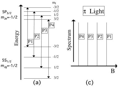
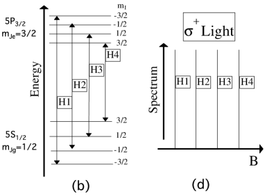
Figure 1: In (a) and (b) energy levels at a given $B$ value. In (c) and (d) the spectrum produced by transitions between the levels of (a) and (b), respectively, at a given laser frequency and scanning the $B$ magnetic field. The top and bottom plots correspond to the nuclear components of different electronic ground/excited states. (a) and (c) correspond to the $|J_{g}=1/2,m_{Jg}=-1/2\rangle\to|J_{e}=3/2,m_{Je}=-1/2\rangle$ $\pi$ transitions, denoted as $\pi$Pi with $(i=1,4)$. (b) and (d) correspond to the $|J_{g}=1/2,m_{Jg}=1/2\rangle\to|J_{e}=3/2,m_{Je}=3/2\rangle$ $\sigma^{+}$ transitions, denoted as $\sigma^{+}$Hi. Notice the energy order of the nuclear levels for different electronic states, producing a different order of the $\pi$Pi and $\sigma^{+}$Hi lines while scanning $B$.

II.2 Absorption lines

The energy levels and the optical transitions are here discussed for the ⁸⁷Rb isotope with $I=3/2$. For a given magnetic field B and a given laser frequency $\nu_{L}$, the absorption spectrum is composed by lines at frequencies

$$\nu_{L}=\nu_{0}+[E_{e}(\frac{3}{2},m_{Je};\frac{1}{2},m_{Ie})-E_{g}(\frac{1}{2},m_{Jg};\frac{3}{2},m_{Ig})],$$ (2)

where $\nu_{0}$ is the rubidium absorption center of gravity at $B=0$, Within the strong magnetic field regimes the light induces mainly transitions with $\Delta m_{I}=0$ selection rules. Because of the small diamagnetic contributions, as in Secs. II.3 and IV.1, the position of absorption lines is dominated by the paramagnetic contributions of Eqs. (1).
Our experimental approach is based on imposing an offset $\Delta\nu_{L}=\nu_{L}-\nu_{0}$ and pulsing the magnetic field from zero to a preset maximum value. At specific times the atoms reach a resonance with the laser by the Zeeman effect. The fluorescence emission monitors the atomic absorption. For our $\Delta\nu_{L}$ positive values, the spectra observed by scanning the magnetic field contain three sets of lines, denoted $\pi$Pi, $\sigma^{+}$Hi, and $\sigma^{+}$Li, starting from a high resonant field to a low one, with $(i=1,4)$ corresponding to the $(m_{I}=\pm 3/2,\pm 1/2)$ components.
The $\pi$ polarized Pi lines, produced by the $|J_{g}=1/2,m_{Jg}=-1/2\rangle\to|J_{e}=3/2,m_{Je}=-1/2\rangle$ transitions, experience the smallest Zeeman shift. Fig. 1(a) shows the energy levels corresponding to these transitions at given $B$. Fig. 1(c) schematizes their nuclear structure as observed at fixed $\Delta\nu_{L}$ and scanning $B$.
Fig. 1(b) shows the energy levels corresponding to the $|J_{g}=1/2,m_{Jg}=1/2\rangle\to|J_{e}=3/2,m_{Je}=3/2\rangle$ $\sigma^{+}$Hi polarized transitions at fixed $B$. The ground state nuclear structure is dominated by the hyperfine interaction even at the highest explored magnetic field, and produces an opposite ranking of the $m_{I}$ levels in Fig. 1(a) and (b) because of the different $m_{Jg}$ sign. The excited state nuclear structure, dominated by the nuclear Zeeman effect, is the same for the two cases. As a consequence scanning the $B$ field, the order of the lines is opposite for the $\pi$Pi and $\sigma^{+}$Hi cases, as in Fig. 1(c) and (d). The centers of gravity of the absorption lines eliminating the hyperfine structure contribution play a key role in our data analysis. For both hyperfine and fine Paschen-Back regimes the center of gravity for the $\sigma^{+}$Hi transitions is

$$B^{H}_{\rm Center}=\frac{\Delta\nu_{L}}{\mu_{B}(3g_{5P_{3/2}}-g_{5S})/2}.$$ (3)

Similar $\sigma^{+}$ transitions denoted $\sigma^{+}$Li are the $|J_{g}=1/2,m_{Jg}=-1/2\rangle\to|J_{e}=3/2,m_{Je}=1/2\rangle$ ones. These transitions appear at a magnetic field lower than the previous ones, because they experience a larger Zeeman shift. The order of the $\sigma^{+}$Li lines observed while scanning the magnetic field is reversed in respect to that of the $\sigma^{+}$Hi lines and similar to the $\pi$Pi ones. For the hyperfine Paschen-Back regime only, the center of gravity of the $\sigma^{+}$Li transitions is

$$B^{L}_{\rm Center}=\frac{\Delta\nu_{L}}{\mu_{B}(g_{5P_{3/2}}+g_{5S})/2}.$$ (4)

Within the hyperfine and fine Paschen-Back regimes, the $\pi$Pi, $\sigma^{+}$Hi, and $\sigma^{+}$Li nuclear transitions are not equally spaced, because of the small excited state hyperfine quadrupole coupling.

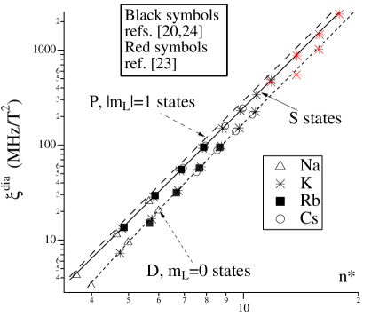
Figure 2: Experimental results and theoretical predictions of $\xi^{dia}$ vs the $n^{*}$ effective quantum number for $S$, $(P,m_{L}=\pm 1)$ and $(D,m_{L}=0)$ low energies states of alkalis. Eq. (6) predictions for those states correspond to the continuous, dashed and dotted lines, respectively. Triangles, stars, filled squares and open circles refer to Na, K, Rb and Cs results, respectively, measured in the references reported within the top box. For our $5S$ and $5P$ states the $n^{*}$ values are 1.81 and 2.30, respectively.

II.3 Diamagnetism

Diamagnetic corrections are necessary for accurate measurements at high magnetic fields. If the magnetic perturbation is smaller than the energy separation between states with different $L$ quantum numbers, the $E^{dia}$ diamagnetic energy for a single valence electron may be written

$$E^{dia}=\xi^{dia}B^{2}\\$$ (5)

on the basis of the susceptibility $\xi^{dia}$. Within an hydrogen-like description, for an electron with quantum numbers $n,L,m_{L}$, and an effective quantum number $n^{*}=n-\delta$ determined by the quantum defect $\delta$, $\xi^{dia}$ derived by Schiff and Snyder (1939); Garstang (1977) was rewritten by Otto et al. (2002) as

$$\xi^{dia}=\frac{5e^{2}a_{0}^{2}}{8\mu_{e}}\left[1+\frac{1-3l(l+1)}{5(n^{*})^{2}}\right]\frac{l(l+1)+m_{l}^{2}-1}{(2l-1)(2l+3)}(n^{*})^{4},$$ (6)

with $a_{0}$ the Bohr radius, $e$ the electron charge and $\mu_{e}$ the electron reduced mass.
Fig. 2 reports experimental determinations and theoretical predictions for $\xi^{dia}$ vs $n^{*}$ in alkalis for low $n$ quantum numbers. Early measurements were performed on P states in Na and K at 2.7 T Jenkins and Segrè (1939) and in K, Rb, Cs at 2.3 T Harting and Klinkenberg (1949). The diamagnetic contribution was measured using two-photon spectroscopy excited S and D states originally by (Harper and Levenson, 1977), and later more systematically for all alkalis by Hüttner et al. (1996); Otto et al. (2002). The measurements by Otto et al. (2002) for $S$ and $D$ states on different alkalis span $n$ quantum numbers as low as three. The simple hydrogen atom description of Eq. ((6)) with quantum defects derived from Gallagher (1994); Li et al. (2003) provides a good fit to the susceptibilities of the figure. The $P$ states measurements by Jenkins and Segrè (1939); Harting and Klinkenberg (1949) on several alkalis focused on quantum numbers between 12 and 30. Those low precision data are also fitted by that equation, except that for Rydberg states with $n>20$ the inter-$L$ perturbation interactions introduce deviations from the predicted values.
Eq. (6) predicts the $\xi^{dia}$ diamagnetic values of 0.29 MHz/T² and 0.68 MHz/T², respectively, for our $5S$ and $5P$ states. That leads to a predicted $\Delta\nu^{dia}=0.39$ MHz/T² diamagnetic shift for the $\sigma^{+}$H4 line, compared to its $\approx 14$ GHz/T paramagnetic shift. All these values should be considered only as an order of magnitude, because of the limited validity of the hydrogen-like description for our states with the low $n^{*}$ values reported in the figure caption. At 58 T the predicted diamagnetic shift is around 1.3 GHz, corresponding to about three times the Doppler linewidth of the absorption lines, whence measurable. Our $\xi^{dia}$ result is presented at the end of Sec. IV.1.

II.4 Data analysis

Our ⁸⁷Rb spectral analysis is based on the atomic constants reported in Steck (2001), except for the Landé $g$-factors. For ⁸⁷Rb the ground state Landé g-factor was precisely measured in Tiedeman and Robinson (1977) with respect to the $g_{e}$ free electron $g$-factor. Making use of the $g_{e}$ value given in Mohr et al. (2016) we obtain $g_{5S}=2.002331070(26).$ A larger indetermination is associated to the Landé $g_{5P_{3/2}}$-factor. The data of Arimondo et al. (1977) point out that for all the alkali atoms the $g$-factor of the first excited $P_{3/2}$ state is $\approx 1.33411$, as predicted by the Russel-Saunders coupling between the orbital magnetic moment, with $g_{L}=1$, and the spin magnetic moment, using $g_{e}$ or $g_{5S}$. For the ⁸⁷Rb $5P_{3/2}$ state, ref. Arimondo et al. (1977) reported 1.3362(13) as a weighted average of all the measurements available at that time and still today. That value is largely determined by fitting the level crossing measurements by Belin and Svanberg Belin and Svanberg (1971), who derived simultaneously $g_{5P_{3/2}}$ and the dipolar and quadrupolar hyperfine constants. We have reanalysed those level-crossing measurements by fixing the hyperfine constants to the very precise values of ref. Ye et al. (1996) reported in Steck (2001) and using the ⁸⁷Rb nuclear magnetic moment of ref. Arimondo et al. (1977). A new $g_{5P_{3/2}}=1.3341(2)$ value is obtained, in agreement with the above Russel-Saunders prediction, to be used as the starting point of our analysis. Following ref. Labzowsky et al. (1999); Goidenko et al. (2002); Indelicato et al. (2007); Gossel et al. (2013), QED and relativistic corrections are at the level of 10^-4-10^-5.

II.5 Rb atom as magnetometer

Our magnetic field determination is based on the rubidium spectrum itself. It relies on the existence of two eigenstates, ground and excited, denoted as extreme, whose energy dependence on the magnetic field is exactly linear, excluding the diamagnetic contribution. These eigenstates correspond to the highest values of all the atomic quantum numbers. The $5^{2}S_{1/2}$ $|J_{g}=1/2,m_{gJ}=1/2;I,m_{gI}=I\rangle$ ground state has the following energy:

$$E_{g}^{+}=\mu_{B}\left(\frac{g_{5S}}{2}+g_{I}I\right)B+\frac{1}{2}A_{g}I.$$ (7)

The excited eigenstate with the highest energy, i.e., the $5P_{3/2}$ $|J_{e}=3/2,m_{eJ}=3/2;I,m_{eI}=I\rangle$ state has the following energy whichever magnetic field value:

$$E_{e}^{+}=\mu_{B}\left(\frac{3g_{5P_{3/2}}}{2}+g_{I}I\right)B+\frac{3}{2}A_{e}I+\frac{1}{4}B_{e}.$$ (8)

These formula for the extreme states, even if derived from Eqs. (1) valid in the hyperfine Paschen-Back regime, apply to all regimes, even for the fine Paschen-Back one.
Combining together Eqs. (2), (7) and  (8), the Zeeman frequency shift of the $\sigma^{+}$H4 optical transition linking the Rb linear dependent states is given by

$$\Delta\nu_{L}(\sigma^{+}H4)=\mu_{B}B\frac{3g_{5P_{3/2}}-g_{5S}}{2}+\frac{I}{2}(3A_{e}-A_{g})+\frac{1}{4}B_{e}.$$ (9)

The inversion of this equation allows to derive the $B$ value from the laser frequency exciting the Rb atoms.
For our Doppler limited spectroscopy with the Gaussian absorption center determined at one twentieth of its linewidth, the magnetic field precision is $\approx 0.002$ T. The above determination leads to the 20 ppm precision at high fields. The Rb magnetometry accuracy is determined by the $g_{5P3/2}$ uncertainty, 750 ppm for the value reported in Arimondo et al. (1977) and 75 ppm for the value derived in Sec. IV.

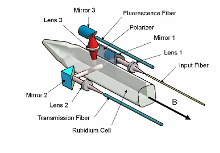
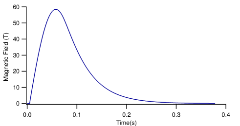
Figure 3: On the top, optical scheme of the Rb cell with a single mode fiber for the laser input and multimode fibers for the transmission light and the fluorescence light output. Matching lenses and a 45^∘ linear polarizer controlling the light reaching the Rb atoms are shown. The cell is oriented parallel to the $B$ field direction and the interrogation light propagates orthogonally to the field. On the bottom, magnetic field temporal dependence for a typical pulse.

III Probe and magnet

The experimental set-up is composed by the rubidium probe located at the center of a solenoid magnet, immersed into liquid nitrogen. The Rb probe is composed by a quartz cell located at the end of a long pipe placing the cell within the magnet and hosting all the electrical and optical connections. The cell with $3\times 3\times 30$ mm³ internal dimensions is filled with natural rubidium. To maintain the cell at room temperature the atomic probe is placed within an evacuated double-walled stainless steel cryostat inserted into the magnet bore. As in the top of Fig. 3, a single mode optical fiber provides the input beam, while the transmitted light and the atomic fluorescence emission reach the outside detectors through multimode fibres. Before entering into the cell the light, generated by a DLX100 Toptica laser, is polarized at 45^∘ with respect to the magnetic field direction in order to induce both $\pi$ and $\sigma$ transitions. The Faraday rotation, experienced by the light propagating through the input single mode fiber and parallely to the magnetic field direction, modifies the total intensity, not the polarization on the atoms. The reported data for a laser intensity fifteen times the saturation intensity are produced by a few ten thousand atoms. Previous tests, performed before assembling the cell within the magnet, demonstrated that the minimum number of detectable atoms is around 100. The fluorescence observation instead of the transmission allows to reduce the influence of the magnetic field inhomogeneity. In fact from the fiber diameter and the collection lens parameters, we evaluate that the fluorescence light is produced from a $0.4\times 0.4\times 0.7$ mm³ volume, smaller than the cell volume probed by transmission.
The 60 T pulsed magnetic field coil, a standard one at the High-Field National Laboratory (LNCMI) in Toulouse, has a 28 mm free bore diameter and is is immersed into the liquid nitrogen in order to facilitate the heat dissipation Debray and Frings (2013). The magnetic field homogeneity on the probed atomic volume is estimated better than 10 ppm. The risetime and decaytime of the field temporal evolutions are around 55 ms and 100 ms, respectively, as shown in the bottom of Fig. 3. The field temporal evolution is monitored by a pick-up coil located at 7 mm from the atoms. Its frequency response bandwidth is larger than 500 kHz. The pick-up signal is calibrated in a separate carefully designed solenoid. The integrated pick-up signal reproduces the time profile of the magnetic pulse. That signal, corrected for the distance from the probe center position, provides a reference measurement $B_{PU}$ of the magnetic field experienced by the atoms. The field calibration is based on the $B_{H4}$ theoretical prediction for the $\sigma^{+}$H4 resonance derived from Eq. (9) at a given laser frequency. From the analysis of $\approx$70 spectra, a linear dependence between $B_{PU}$ and $B_{H4}$ was verified, with slope $0.9899(2)$ using the Russell-Saunders $g$-factor reported above. For a more detailed set-up description see George et al. (2017).

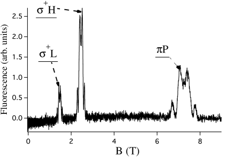
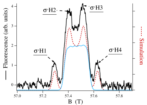
Figure 4: Rb fluorescence spectra observed by scanning the magnetic field, on the top for $\Delta\nu_{L}=34.692(5)$ and on the bottom for $\Delta\nu_{L}=812.331(5)$, all in GHz, with uncertainty given by the accuracy of the wavelength meter reading. For both spectra the sinusoidal periodic fluorescence variation produced by the fiber Faraday effect was subtracted. The bottom plot, on an expanded scale, shows the individual $\sigma^{+}$Hi lines for a very high magnetic field. The quantum number assignment is in Fig. 1. Each fluorescent structure is composed by four resolved lines associated to the ⁸⁷Rb nuclear spin states and by a central unresolved broad structure associated to the ⁸⁵Rb nuclear components. The dotted red line reports a simulation including the Gaussian Doppler broadening for each absorption line, while the blue continuous line reports only the ⁸⁵Rb contribution, with an offset for both of them, for presentation clarity. The simulation only free parameter is the overall scale.

IV Experimental results

IV.1 Spectra

Examples of the observed fluorescence spectra are reported in Fig. 4 for two different values of the $\Delta\nu_{L}$ while the magnetic field is scanned during the pulse decaytime. Similar spectra are obtained while the magnetic field is scanned up. The top spectrum, obtained for a low $\Delta\nu_{L}$, is characterized by the presence of all the $\sigma^{+}$Li, $\sigma^{+}$Hi and $\pi$Pi lines in sequence at increasing $B$ values. The lines at higher $B$ values experience a smaller Zeeman shift. The intensities are proportional to the theoretically predicted line strengths. In the bottom spectrum, obtained for a large $\Delta\nu_{L}$, the $\sigma^{+}$Hi lines appears for a magnetic field close to the coil maximum operational current. The horizontal scales are obtained combining the information provided by the $B_{H4}$ value and the temporal magnetic field dependence measured by the pick-up coil.
Each fluorescent set includes the ⁸⁵Rb and ⁸⁷Rb contributions. The four peak structure observed for each set corresponds to the nuclear structure of the ⁸⁷Rb $I=3/2$ spin. Because for ⁸⁵Rb the $A_{g}$ hyperfine coupling is two times smaller than for ⁸⁷Rb, and because of its higher spin value $I=5/2$, the nuclear structure cannot be resolved by the Doppler limited spectroscopy. We have performed simulations of the spectra including the Doppler Gaussian broadening, an example represented by the red dotted line of Fig. 4 bottom. The simulation reproduces the four ⁸⁷Rb $\sigma^{+}$Hi lines having the same intensity and the central broadening due to the unresolved ⁸⁵Rb lines. On the bottom spectrum, the asymmetry between the two sides of the absorption structure, clearly visible on the ⁸⁵Rb simulation, is produced by the unequal spacing among the nuclear levels, around 0.002 T in the resonant magnetic field.
Analysing spectra obtained for different $\Delta\nu_{L}$ values, we derive the linear relation between $B_{PU}$ and $B_{H4}$ reported within Sec. III. In order to test the presence of a quadratic diamagnetic nonlinearity, we repeat the previous analysis of $B_{PU}$ vs $B_{H4}$ by including into the fit function a quadratic term. The fit quality is not improved and the derived $\xi^{dia}$ value is smaller than the above theoretical prediction by a factor ten and compatible with zero owing to a large error bar.

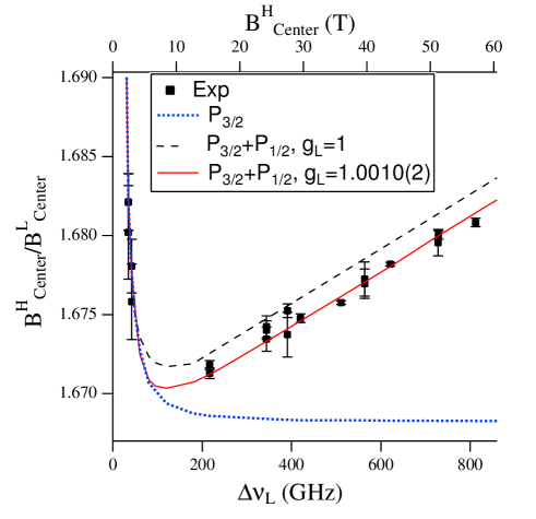
Figure 5: Ratio between $BH_{\rm Center}$ and $BL_{\rm Center}$ magnetic fields versus the $\Delta\nu_{L}$ laser detuning (bottom axis) and $BH_{\rm Center}$ value (top axis). Squares for the measured values, including error bars, in several cases smaller than the square. Lines report theoretical predictions. The dotted blue line is based on the 5²P_3/2 eigenergies, at high magnetic fields leading to the hyperfine Paschen-Back regime with a constant value of the ratio. The black dashed line and the red continuous line are based on the magnetic eigenenergies of the whole fine structure 5²P_3/2 and 5²P_1/2 manifold, describing at high fields the fine Pachen-Back regime. Different $g_{L}$-values, shown in the inset, with $g_{S}=g_{5S}$, are used for the two cases. The red line results are obtained also for other $[g_{L}$, $g_{S}]$ combinations discussed in the text.

IV.2 Ratio between $B^{H}_{\rm Center}$ and $B^{L}_{\rm Center}$

This Subsection targets the $g_{5P_{3/2}}$ value that among the Rb data has a low accuracy. Eqs. (3) and  (4) show the different dependence of $B^{H}_{\rm Center}$ and $B^{L}_{\rm Center}$ on $g_{5P_{3/2}}$ because of the different excited state $m_{Je}$ quantum numbers. Those equations don’t have the same regime of validity: the $B^{H}_{\rm Center}$ expression is valid at all fields; the $B^{L}_{\rm Center}$ is based on the hyperfine Paschen-Back approximation. Within this approximation, at high magnetic fields, for a given $\Delta\nu_{L}$ laser detuning the $B^{H}_{\rm Center}/B^{L}_{\rm Center}$ ratio is a constant. This prediction is shown by the dotted blue line in Fig. 5 where also the experimental results for the ratio are plotted as function of $\Delta\nu_{L}$ on the bottom axis, or the corresponding $B^{H}_{\rm Center}$ center on the top axis. Notice the high precision reached by the measurements at very high fields, where the Doppler linewidth is a small fraction of the Zeeman shift. Our data do not follow the constant value theoretically predicted by the dotted line of the hyperfine Paschen-Back description. Instead the ratio increases with the $\Delta\nu_{L},B^{H}_{\rm Center}$ values.
After excluding technical issues, as the shift of the probe position within the magnet at very high fields, we have searched a different explanation. As in Sec. IIA, for the rubidium first resonance line the fine Paschen-Back regime is fully reached for a magnetic field around 500 T. Fig. 5 explores a range of $B$ values lower than this limit. Nevertheless we have calculated the eigenergies of all the fine structure levels, i.e., both 5${}^{2}P_{3/2}$ and 5${}^{2}P_{1/2}$ states, including the hyperfine outdiagonal matrix elements as in ref. Arimondo et al. (1977). The operating magnetic field, ”low” for fully reaching the fine Paschen-Back regime, produces a deviation of the $|5^{2}P_{3/2};J_{e}=3/2,m_{Je}=1/2;I,m_{Ie}\rangle$ energies (those of the $\sigma^{+}$Li transitions) from the hyperfine Paschen-Back prediction, at the $\approx 10^{-4}$ level. As a consequence also the $B^{H}_{\rm Center}/B^{L}_{\rm Center}$ ratio is modified.
As starting point, the theoretical analysis for the fine Paschen-Back regime is based on the orbital Landé $g_{L}$-factor equal 1 and the spin $g_{S}$-factor equal to $g_{5S}$, leading within the Russell-Saunders coupling to the $g_{5P_{3/2}}$ value presented in Section II.4. This analysis, represented in Fig. 5 by the black dashed line, reproducing the observed behaviour at low magnetic fields, agrees qualitatively with the measured increase at high magnetic fields.
By exploring the role of the $g$-factor values on the high field slope of the $B^{H}_{\rm Center}/B^{L}_{\rm Center}$ ratio, we find that the experimental data can be reproduced by modifying $g_{L}$ and $g_{S}$. Several contributions modify those values, as perturbations by excited core states Phillips (1952), configuration mixing Childs and Goodman (1971), combined action of exchange core polarization and spin-orbit interaction Gossel et al. (2013), relativistic and QED corrections  Labzowsky et al. (1999); Goidenko et al. (2002); Indelicato et al. (2007); Gossel et al. (2013). By scanning the $[g_{L},g_{S}]$ plane we reach a good agreement between theory and experiment as shown by the red continuous line in Fig 5. The data are fitted by all the values lying on the line segment bounded by the $[1.0012(2),g_{5S}]$ and $[1.,2.0049(2)]$ points. The first extreme assumes that an atomic perturbation modifies the $g_{L}$-factor of the $5P$ state without modification of $g_{S}$. The second extreme assumes no perturbation on $g_{L}$ and a $g_{S}$ increase larger than the predicted relativistic and QED corrections. Because our single result cannot discriminate between all these mechanisms, only an atomic physics theoretical calculation may determine the precise corrections for the $g$-factors. The $[g_{L},g_{S}]$ combinations lying on the above segment lead to very close values for the $5P_{3/2}$ Landé factor globally described by

$$g_{5P_{3/2}}=1.33494(15),$$ (10)

with included error propagation. This value lies between the one reported in the review Arimondo et al. (1977) and that derived in Sec. II.4 from our reanalysis of the level crossing of Belin and Svanberg (1971). It is more precise than both of them.
Owing to the $5\times 10^{-4}$ fractional difference between the above $g_{5P_{3/2}}$ value and the Russel-Saunders starting value, the linear relation between $B_{PU}$ and $B_{H4}$ of Sec. III is modified by a quantity roughly equal to the the error bar of that relation.

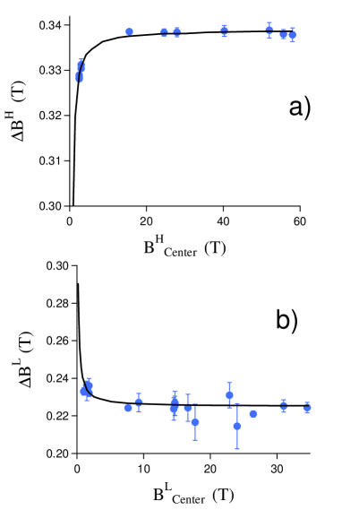
Figure 6: Hyperfine interaction splitting of the $\sigma^{+}$Hi absorption lines, in (a), and $\sigma^{+}$Li, in (b), versus the magnetic field center of those lines. Dots for the experimental data with their error bars, and theoretical predictions derived from the Hamiltonan eigenenergies. The constant values at high field correspond to the predictions of the hyperfine/fine Paschen-Back regime. The $g_{5P_{3/2}}$ value of Eq. (10) is inserted into the theoretical analysis.

IV.3 Hyperfine structure

As a test of the comparison between experimental results and theoretical predictions, we have examined the magnetic field separations between the nuclear components of the $\sigma^{+}$Hi and $\sigma^{+}$Li lines. We have measured the ⁸⁷Rb quantities $\Delta B^{\mathrm{H}}=B_{\rm H4}-B_{\mathrm{H}1}$ and $\Delta B^{\mathrm{L}}=B_{\mathrm{L}1}-B_{\mathrm{L}4}$ as a function of $BH_{\mathrm{C}enter}$ and $BL_{\mathrm{C}enter}$, respectively. The data and the theoretical predictions are plotted in Fig. 6. For the few experimental data having large error bars, the input fiber Faraday rotation reduces the fluorescence signal intensity and deteriorates the spectra fitting procedure. The nuclear structure is entirely produced by the hyperfine coupling between electronic and nuclear spins, because owing to the $\Delta m_{I}=0$ selection the nuclear Zeeman energy does not modify the resonant frequency. Within the hyperfine Paschen-Back regime where $\mathbf{J}$ and $\mathbf{I}$ are fully decoupled, the $m_{I}$ levels are nearly equally spaced, producing a constant frequency separation, as shown in Figs. 1 (b) and (d). That is not true at the low $B$ fields where $\mathbf{F}$ is the good quantum number. This difference explains why the theoretical curves rise up or fall down before saturating to a well defined value. The experimental/theoretical agreement demonstrates the precision of our measurements and the correctness of the atomic eigenenergy derivation.
The hyperfine Paschen-Back regime is reached for $\mu_{B}B$ larger than the ground state hyperfine splitting. For rubidium Sec. II.1 places this transition around 0.5 T. Instead the data of Fig. 6 demonstrate that the transition takes place at different magnetic fields, starting roughly around 0.4 T or 1.5 T depending on the observable, and terminating at higher fields. The excited state Landé $g$-factor determines the magnetic field amplitudes where constant values of $\Delta B^{\mathrm{H}}$ and $\Delta B^{\mathrm{L}}$ are reached. However the smooth transitions between the different regimes and our error bars do not allow a determination of the $g$-factor. Notice that while the $g$-factor of Eq. (10) was used for the theoretical predictions of the figure, the use of the Russell-Saunders produces theoretical curves modified on their high-field value, but with no visible modification in the transition regions.

V Conclusion

We have performed high resolution spectroscopy of a rubidium optical transition at a field slightly larger than 58 T. Our Rb sensor shows performances more than an order of magnitudes better than standard pick-up coils in terms of uncertainty, compactness and direct access to a micrometer size explored region.
The high precision data collected in a two-week run at the LNCMI facility allowed an investigation of the atomic response for high magnetic fields not fully explored previously. We have investigated in detail the transition between different magnetic regimes. We were forced to analyze theoretically our data on the basis of a treatment typically applied only to the fine Paschen-Back regime, even operating at magnetic fields lower than those naively associated to that regime. The focus of our experiment was to test rubidium atom as a magnetometer, therefore we have not accumulated enough data, as for the Pi lines, and none for the $\sigma^{-}$ transitions. A complete investigation will increase the precision of the measured excited state Landé $g$-factor.
While our work relies on the Doppler limited absorption spectroscopy, the application of sub-Doppler spectroscopy will lead to an increased resolution by a factor hundred. In our setup the observation of sub-Doppler absorption features relies on technical improvements. Another straightforward way to improve the probe precision is to operate with a cell containing a single rubidium isotope.
Our rubidium magnetometry accuracy is presently limited by the $g_{5P3/2}$ value, whose precision even if improved by us cannot yet compete with the hydrogen nuclear magnetic resonance. When the precision of the $g$-factor and of the diamagnetic corrections will be improved, the Rb magnetometer accuracy could compete with the hydrogen NMR magnetometer.
Our results opens the way to dilute matter optical tests in high magnetic fields. Precise measurements of $g$-factors of excited states at a level interesting to verify QED predictions appear feasible. The use of other atomic transitions or of very narrow optical transitions as in alkaline-earths will expand the atomic physics at high magnetic fields and its applications.

References

- Kominis et al. (2003) I. K. Kominis, T. W. Kornack, J. C. Allred, and M. V. Romalis, Nature 422, 596 (2003).
- Vengalattore et al. (2007) M. Vengalattore, J. M. Higbie, S. R. Leslie, J. Guzman, L. E. Sadler, and D. M. Stamper-Kurn, Phys. Rev. Lett. 98, 200801 (2007).
- Mamin et al. (2007) H. J. Mamin, M. Poggio, C. L. Degen, and D. Rugar, Nat Nano 2, 301 (2007).
- Taylor et al. (2008) J. M. Taylor, P. Cappellaro, L. Childress, L. Jiang, D. Budker, P. R. Hemmer, A. Yacoby, R. Walsworth, and M. D. Lukin, Nat. Phys. 4, 810 (2008).
- Pham et al. (2011) L. M. Pham, D. L. Sage, P. L. Stanwix, T. K. Yeung, D. Glenn, A. Trifonov, P. Cappellaro, P. R. Hemmer, M. D. Lukin, H. Park, A. Yacoby, and R. L. Walsworth, NJP 13, 045021 (2011).
- Rondin et al. (2014) L. Rondin, J.-P. Tetienne, T. Hingant, J.-F. Roch, P. Maletinsky, and V. Jacques, Rep. Progr. Phys. 77, 056503 (2014).
- Budker and Kimball (2013) F. Budker, D. Derek and J. Kimball, Optical Magnetometry (Cambridge University Press, 2013).
- Garn et al. (1966) W. B. Garn, R. S. Caird, D. B. Thomson, and C. M. Fowler, Rev. Sci. Instrum. 37, 762 (1966).
- Hori et al. (1982) H. Hori, M. Miki, and M. Date, J. Phys. Soc. Japan 51, 1566 (1982).
- Gomez et al. (2014) M. R. Gomez, S. B. Hansen, K. J. Peterson, D. E. Bliss, A. L. Carlson, D. C. Lamppa, D. G. Schroen, and G. A. Rochau, Rev. Sci. Instrum. 85, 11E609 (2014).
- Banasek et al. (2016) J. T. Banasek, J. T. Engelbrecht, S. A. Pikuz, T. A. Shelkovenko, and D. A. Hammer, Rev. Sci. Instrum. 87, 103506 (2016).
- George et al. (2017) S. George, N. Bruyant, J. B. Béard, S. Scotto, E. Arimondo, R. Battesti, D. Ciampini, and C. Rizzo, Rev. Sci. Instrum. 88, 073102 (2017).
- Kopfermann (1958) H. Kopfermann, Nuclear Moments (Academic Press, New York, 1958).
- (14) S. J. Lipson, G. D. Fletcher, and D. J. Larson, Phys. Rev. Lett. 57, 567.
- (15) N. Fortson, Phys. Rev. Lett. 59, 988.
- Arimondo et al. (1977) E. Arimondo, M. Inguscio, and P. Violino, Rev. Mod. Phys. 49, 31 (1977).
- Foot (2012) C. Foot, Atomic Physics (Oxford University Press, 2012).
- Schiff and Snyder (1939) L. Schiff and H. Snyder, Phys. Rev. 55, 59 (1939).
- Garstang (1977) R. Garstang, Rep. Progr. Phys. 40, 105 (1977).
- Otto et al. (2002) P. Otto, M. Gamperling, M. Hofacker, T. Meyer, V. Pagliari, A. Stifter, M. Krauss, and W. Hüttner, Chem. Phys. 282, 289 (2002).
- Jenkins and Segrè (1939) F. Jenkins and E. Segrè, Phys. Rev. 55, 52 (1939).
- Harting and Klinkenberg (1949) D. Harting and P. Klinkenberg, Physica 14, 669 (1949).
- Harper and Levenson (1977) C. Harper and M. Levenson, Opt. Commun. 20, 107 (1977).
- Hüttner et al. (1996) W. Hüttner, P. Otto, and M. Gamperling, Phys. Rev. A 54, 1318 (1996).
- Gallagher (1994) T. Gallagher, Rydberg Atoms (Cambridge University Press, 1994).
- Li et al. (2003) W. Li, I. Mourachko, M. Noel, and T. Gallagher, Phys. Rev. A 67, 052502 (2003).
- Steck (2001) D. Steck, “Rubidium 87 D line data, 2001,” (2001).
- Tiedeman and Robinson (1977) J. S. Tiedeman and H. G. Robinson, Phys. Rev. Lett. 39, 602 (1977).
- Mohr et al. (2016) P. J. Mohr, D. B. Newell, and B. N. Taylor, Rev. Mod. Phys. 88, 035009 (2016).
- Belin and Svanberg (1971) G. Belin and S. Svanberg, Physica Scripta 4, 269 (1971).
- Ye et al. (1996) J. Ye, S. Swartz, P. Jungner, and J. L. Hall, Opt. Lett. 21, 1280 (1996).
- Labzowsky et al. (1999) L. Labzowsky, I. Goidenko, and P. Pyykkö, Phys. Lett. A 258, 31 (1999).
- Goidenko et al. (2002) I. Goidenko, L. Labzowsky, G. Plunien, and G. Soff, Phys. Rev. A 66, 032115 (2002).
- Indelicato et al. (2007) P. Indelicato, J. P. Santos, S. Boucard, and J.-P. Desclaux, Eur. Phys. J. D 45, 155 (2007).
- Gossel et al. (2013) G. H. Gossel, V. A. Dzuba, and V. V. Flambaum, Phys. Rev. A 88, 034501 (2013).
- Debray and Frings (2013) F. Debray and P. Frings, C. R. Phys. 14, 14 (2013).
- Phillips (1952) M. Phillips, Phys. Rev. 88, 202 (1952).
- Childs and Goodman (1971) W. J. Childs and L. S. Goodman, Phys. Rev. A 3, 25 (1971).