PROBE-GK: Predictive Robust Estimation using Generalized Kernels

Abstract

Many algorithms in computer vision and robotics make strong assumptions about uncertainty, and rely on the validity of these assumptions to produce accurate and consistent state estimates. In practice, dynamic environments may degrade sensor performance in predictable ways that cannot be captured with static uncertainty parameters. In this paper, we employ fast nonparametric Bayesian inference techniques to more accurately model sensor uncertainty. By setting a prior on observation uncertainty, we derive a predictive robust estimator, and show how our model can be learned from sample images, both with and without knowledge of the motion used to generate the data. We validate our approach through Monte Carlo simulations, and report significant improvements in localization accuracy relative to a fixed noise model in several settings, including on synthetic data, the KITTI dataset, and our own experimental platform.

I Introduction

Modern ground, aerial, and underwater vehicles are able to carry exteroceptive sensors capable of observing the world with high spatial and temporal resolution. Despite steady improvements in computing power, it remains impractical in many situations for robots to reason directly over all of the available sensor data. Instead, it is common to use feature extraction and interest point detection algorithms to provide a simplified representation of the environment, and to perform tasks like odometry and mapping using that simplified feature-based representation.

However, not all features are created equal; most feature-based methods rely on random sample consensus algorithms [1] to partition the extracted features into inliers and outliers, and perform estimation based only on inliers. It is common to guard against misclassifying an outlier as an inlier by using robust estimation techniques, such as the Cauchy costs employed in [2] or the dynamic covariance scaling devised by [3]. These approaches, often grouped under the title of M-estimation, aim to maintain a quadratic influence of small errors, while reducing the contribution of larger errors. The robustness and accuracy of feature-based visual odometry often hinges on the tuning of the parameters of inlier selection and robust estimation. Performance can vary significantly from one environment to the next, and most algorithms require careful tuning to work in a given environment.

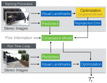
Figure 1: Our proposed system builds a predictive noise model for stereo visual odometry. (a) At training time, we extract landmarks from two pairs of stereo images, and use egomotion ground truth to compute reprojection errors to build a covariance model. (b) At run time, we predict a covariance for each visual landmark. We use these covariances in a robust nonlinear least-squares problem, which is solved to estimate the transform between camera poses. (c) If the ground truth egomotion is not known, we iteratively apply an optimization procedure (yellow box) to estimate them.

In this paper, we describe a principled, data-driven way to build a noise model for visual odometry. We combine our previous work [4] on predictive robust estimation (PROBE) with our work on covariance estimation [5] to formulate a predictive robust estimator for a stereo visual odometry pipeline. We frame the traditional non-linear least squares optimization problem as a problem of maximum likelihood estimation with a Gaussian noise model, and infer a distribution over the covariance matrix of the Gaussian noise from a predictive model learned from training data. This results in a Student’s $t$ distribution over the noise, and naturally yields a robust nonlinear least-squares optimization problem. In this way, we can predict, in a principled manner, how informative each visual feature is with respect to the final state estimate, which allows our approach to intelligently weight observations to produce more accurate odometry estimates. Our pipeline is outlined in Figure 1.

The central contributions of our paper are:

1. a probabilistic model for sparse stereo visual odometry, leading to a predictive robust algorithm for inference on that model,

2. a procedure for training our model using pairs of stereo images with known relative transform, and

3. an iterative, expectation-maximization approach to train our model when the relative ground truth egomotion is unavailable.

II System Overview

II-A Sparse stereo visual odometry

In our frame-to-frame sparse stereo odometry pipeline, the objective is to find $\mathcal{T}_{t}\in\text{SE}(3)$, the rigid transform between two subsequent stereo camera poses (note that the temporal index $t$ refers to the set of two stereo camera poses). We begin by rectifying, then stereo and temporally matching the set of 4 images to generate the corresponding locations of a set of $N_{t}$ visual landmarks in each stereo pair. Each landmark corresponds to a point in space, expressed in homogeneous coordinates in the camera frame as $\boldsymbol{p}_{i,t}:={\begin{bmatrix}p_{1}&p_{2}&p_{3}&p_{4}\end{bmatrix}}^{\top}\in\mathbb{P}^{3}$. The stereo-camera model, $f$, projects a landmark expressed in homogeneous coordinates into image space, so that $\mathbf{\boldsymbol{y}}_{i,t}$, the stereo pixel coordinates of landmark $i$ in the first camera pose at time $t$, is given by

$$\mathbf{\boldsymbol{y}}_{i,t}=\begin{bmatrix}u_{l}\\ v_{l}\\ u_{r}\\ v_{r}\end{bmatrix}=f(\boldsymbol{p}_{i,t})=\mathbf{M}\frac{1}{p_{3}}\boldsymbol{p}_{i,t},$$ (1)

where

$$\mathbf{M}=\begin{bmatrix}f_{u}&0&c_{u}&f_{u}\frac{b}{2}\\ 0&f_{v}&c_{v}&0\\ f_{u}&0&c_{u}&-f_{u}\frac{b}{2}\\ 0&f_{b}&c_{v}&0\end{bmatrix}.$$ (2)

Here, $\{c_{u},c_{v}\}$, $\{f_{u},f_{v}\}$, and $b$ are the principal points, focal lengths and baseline of the stereo camera respectively. Note that in this formulation, the stereo camera frame is centered between the two individual lenses.

We triangulate landmarks in the first camera frame, $\mathbf{\boldsymbol{y}}_{i,t}$, and re-project them into the second frame, $\mathbf{\boldsymbol{y}}_{i,t}^{\prime}$. We model errors due to sensor noise and quantization as a Gaussian distribution in image space with a known covariance $\mathbf{R}$,

$$p(\mathbf{\boldsymbol{y}}_{i,t}^{\prime}|\mathbf{\boldsymbol{y}}_{i,t},\mathcal{T}_{t},\mathbf{R})=\mathcal{N}\left(\mathbf{\boldsymbol{e}}_{i,t}(\mathcal{T}_{t});\mathbf{\boldsymbol{0}},\mathbf{R}\right),$$ (3)

where

$$\mathbf{\boldsymbol{e}}_{i,t}=\mathbf{\boldsymbol{y}}_{i,t}^{\prime}-f(\mathcal{T}_{t}f^{-1}(\mathbf{\boldsymbol{y}}_{i,t})).$$ (4)

The maximum likelihood transform, $\mathcal{T}_{t}^{*}$, is then given by

$$\mathcal{T}_{t}^{*}=\underset{\mathcal{T}_{t}\in\text{SE}(3)}{\text{arg\,min}}\,\sum_{i=1}^{N_{t}}{\mathbf{\boldsymbol{e}}_{i,t}}^{\top}\mathbf{R}^{-1}\mathbf{\boldsymbol{e}}_{i,t}.$$ (5)

This is a nonlinear least squares problem, and can be solved iteratively using standard techniques. During iteration $n$, we represent the transform as the product of an estimate $\mathcal{T}^{(n)}\in\text{SE}(3)$ and a perturbation $\delta\mathbf{\boldsymbol{\xi}}\in\mathbb{R}^{6}$ represented in exponential coordinates:

$$\mathcal{T}_{t}=\exp{\left(\delta\mathbf{\boldsymbol{\xi}}^{\wedge}\right)}\mathcal{T}_{t}^{(n)}.$$ (6)

The wedge operator $(\cdot)^{\wedge}$ is defined (following [6]) as both the map $\mathbb{R}^{3}\to\mathfrak{so}(3)$,

$$\mathbf{\boldsymbol{\phi}}^{\wedge}\triangleq\begin{bmatrix}\phi_{1}\\ \phi_{2}\\ \phi_{3}\end{bmatrix}^{\wedge}=\begin{bmatrix}0&-\phi_{3}&\phi_{2}\\ \phi_{3}&0&-\phi_{1}\\ -\phi_{2}&\phi_{1}&0\end{bmatrix},$$ (7)

and the map $\mathbb{R}^{6}\to\mathfrak{se}(3)$,

$$\mathbf{\boldsymbol{\xi}}^{\wedge}\triangleq\begin{bmatrix}\mathbf{\boldsymbol{\rho}}\\ \mathbf{\boldsymbol{\phi}}\end{bmatrix}^{\wedge}=\begin{bmatrix}\mathbf{\boldsymbol{\phi}}^{\wedge}&\mathbf{\boldsymbol{\rho}}\\ {\mathbf{\boldsymbol{0}}}^{\top}&0\end{bmatrix}.$$ (8)

Linearizing the transform for small perturbations $\delta\mathbf{\boldsymbol{\xi}}$ yields a linear least-squares problem:

$$\mathcal{L}(\delta\mathbf{\boldsymbol{\xi}})=\frac{1}{2}\sum_{i=1}^{N_{t}}{\left(\mathbf{\boldsymbol{e}}_{i,t}^{(n)}-\mathbf{J}_{i,t}^{(n)}\delta\mathbf{\boldsymbol{\xi}}\right)}^{\top}\mathbf{R}^{-1}\left(\mathbf{\boldsymbol{e}}_{i,t}^{(n)}-\mathbf{J}_{i,t}^{(n)}\delta\mathbf{\boldsymbol{\xi}}\right)$$ (9)

Here, $\mathbf{J}_{i,t}^{(n)}$ is the Jacobian matrix of the reprojection error. The explicit form of the Jacobian matrix is omitted for brevity but can be found in our supplemental materials.

Rearranging, we see the minimizing perturbation is the solution to a linear system of equations:

$$\delta\mathbf{\boldsymbol{\xi}}^{(n)}=\left(\sum_{i=1}^{N_{t}}{\mathbf{J}}^{\top}_{i,t}\mathbf{R}_{,}^{-1}\mathbf{J}_{i,t}\right)^{-1}\sum_{i=1}^{N_{t}}{\mathbf{J}}^{\top}_{i,t}\mathbf{R}^{-1}\mathbf{\boldsymbol{e}}_{i,t}^{(n)}.$$ (10)

We then update the estimated transform and proceed to the next iteration.

$$\mathcal{T}_{t}^{(n+1)}=\exp{\left(\delta\mathbf{\boldsymbol{\xi}}^{(n)\wedge}\right)}\mathcal{T}_{t}^{(n)}.$$ (11)

There are many reasonable choices for both the initial transform $\mathcal{T}_{t}^{(0)}$ and for the conditions under which we terminate iteration. We initialize the estimated transform to identity, and iteratively perform the update given by eq. 11 until we see a relative change in the squared error of less than one percent after an update.

II-B Predictive noise models for visual odometry

The process described in the previous section employs a fixed noise covariance $\mathbf{R}$. However, not all landmarks are created equal: differing texture gradients can cause feature localization to degrade in predictable ways, and effects like motion blur can lead to landmarks being less informative. If we had a good estimate of the noise covariance for each landmark, we could simply replace the fixed covariance $\mathbf{R}$ with one that varies for each stereo observation, $\mathbf{R}_{i,t}$. Such a predictive model would allows us to better account for observation errors from a diverse set of noise sources, and incorporate information from landmarks that may otherwise be discarded by a binary outlier rejection scheme.

However, estimating these covariances in a principled way is a nontrivial task. Even when we have reasonable heuristic estimates available, it is difficult to guarantee those estimates will be reliable. Instead of relying solely on such heuristics, we propose to learn these image-space noise covariances from data.

We associate with each landmark $\mathbf{\boldsymbol{y}}_{i,t}$ a vector of predictors, $\mathbf{\boldsymbol{\phi}}_{i,t}\in\mathbb{R}^{M}$. Each predictor can be computed using both visual and inertial cues, allowing us to model effects like motion blur and self-similar textures. We then compute the covariance as a function of these predictors, so that $\mathbf{R}_{i,t}=\mathbf{R}(\mathbf{\boldsymbol{\phi}}_{i,t})$. In order to exploit conjugacy to a Gaussian noise model, we formulate our prior knowledge about this function using an inverse Wishart (IW) distribution over positive definite $d\times d$ matrices (the IW distribution has been used as a prior on covariance matrices in other robotics and computer vision contexts, see for example, [7]). This distribution is defined by a scale matrix $\mathbf{\Psi}\in\mathbb{R}^{d\times d}\succ 0$ and a scalar quantity called the degrees of freedom $\nu\in\mathbb{R}>d-1$:

$$p\left(\mathbf{R}\right) =\text{IW}\left(\mathbf{R};\mathbf{\Psi},\nu\right)$$ (12)

$$=\frac{|\mathbf{\Psi}|^{\nu/2}}{2^{\frac{\nu d}{2}}\Gamma_{d}(\frac{\nu}{2})}|\mathbf{R}|^{-\frac{\nu+d+1}{2}}\exp\left(-\frac{1}{2}\text{tr}\left(\mathbf{\Psi}\mathbf{R}^{-1}\right)\right).$$

We use the scale matrix to encode our prior estimate of the covariance, and the degrees of freedom to encode our confidence in that estimate. Specifically, if we estimate the covariance $\mathbf{R}$ associated with predictor $\mathbf{\boldsymbol{\phi}}$ to be $\hat{\mathbf{R}}$ with a confidence equivalent to seeing $n$ independent samples of the error from $\mathcal{N}(\mathbf{\boldsymbol{0}},\hat{\mathbf{R}})$, we would choose $\nu(\mathbf{\boldsymbol{\phi}})=n$ and $\mathbf{\Psi}(\mathbf{\boldsymbol{\phi}})=n\hat{\mathbf{R}}$.

Given a sequence of observations and ground truth transformations,

$$\mathcal{D}=\{\mathcal{I}_{t},\mathcal{T}_{t}\},\quad t\in[1,N]$$ (13)

where

$$\mathcal{I}_{t}=\{\mathbf{\boldsymbol{y}}_{i,t},\mathbf{\boldsymbol{y}}_{i,t}^{\prime},\mathbf{\boldsymbol{\phi}}_{i,t}\}\quad i\in[1,N_{t}],$$ (14)

we can use the procedure of generalized kernel estimation [8] to infer a posterior distribution over the covariance matrix $\mathbf{R}_{*}$ associated with some query predictor vector $\mathbf{\boldsymbol{\phi}}_{*}$:

$$p(\mathbf{R}_{*}|\mathcal{D},\mathbf{\boldsymbol{\phi}}_{*}) \propto\prod_{i,t}\mathcal{N}(\mathbf{\boldsymbol{e}}_{i,t}|\mathbf{\boldsymbol{0}},\mathbf{R}_{*})^{k(\mathbf{\boldsymbol{\phi}}_{*},\mathbf{\boldsymbol{\phi}}_{i,t})}$$

$$\qquad\times\text{IW}(\mathbf{R}_{*};\mathbf{\Psi}(\mathbf{\boldsymbol{\phi}}_{*}),\nu(\mathbf{\boldsymbol{\phi}}_{*}))$$ (15)

$$=\text{IW}(\mathbf{R}_{*};\mathbf{\Psi}_{*},\nu_{*}).$$ (16)

Here, $\mathbf{\boldsymbol{e}}_{i,t}=\mathbf{\boldsymbol{y}}_{i,t}^{\prime}-f(\mathcal{T}_{t}f^{-1}(\mathbf{\boldsymbol{y}}_{i,t}))$ as before. The function $k:\mathbb{R}^{M}\times\mathbb{R}^{M}\to[0,1]$ is a kernel function which measures the similarity of two points in predictor space. Note also that the posterior parameters $\mathbf{\Psi}_{*}$ and $\nu_{*}$ can be computed in closed form as

$$\mathbf{\Psi}_{*} =\mathbf{\Psi}(\mathbf{\boldsymbol{\phi}}_{*})+\sum_{i,t}k(\mathbf{\boldsymbol{\phi}}_{*},\mathbf{\boldsymbol{\phi}}_{i,t})\mathbf{\boldsymbol{e}}_{i,t}{\mathbf{\boldsymbol{e}}_{i,t}}^{\top},$$ (17)

$$\nu_{*} =\nu(\mathbf{\boldsymbol{\phi}}_{*})+\sum_{i,t}k(\mathbf{\boldsymbol{\phi}}_{*},\mathbf{\boldsymbol{\phi}}_{i,t}).$$ (18)

If we marginalize over the covariance matrix, we find that the posterior predictive distribution is a multivariate Student’s $t$ distribution:

$$p(\mathbf{\boldsymbol{y}}_{i,t}^{\prime} |\mathcal{T}_{t},\mathbf{\boldsymbol{y}}_{i,t},\mathcal{D},\mathbf{\boldsymbol{\phi}}_{i,t})$$ (19)

$$=\int\mathrm{d}\mathbf{R}_{i,t}\mathcal{N}\left(\mathbf{\boldsymbol{e}}_{i,t};\mathbf{\boldsymbol{0}},\mathbf{R}_{i,t}\right)\text{IW}(\mathbf{R}_{i,t};\mathbf{\Psi}_{*},\nu_{*})$$ (20)

$$=\text{t}_{\nu_{*}-d+1}\left(\mathbf{\boldsymbol{e}}_{i,t};\mathbf{\boldsymbol{0}},\frac{1}{\nu_{*}-d+1}\mathbf{\Psi}_{*}\right)$$ (21)

$$=\frac{\Gamma(\frac{\nu_{*}+1}{2})}{\Gamma(\frac{\nu_{*}-d+1}{2})}|\mathbf{\Psi_{*}}|^{-\frac{1}{2}}\pi^{-\frac{d}{2}}\left(1+{\mathbf{\boldsymbol{e}}_{i,t}}^{\top}\mathbf{\Psi_{*}}^{-1}\mathbf{\boldsymbol{e}}_{i,t}\right)^{-\frac{\nu_{*}+1}{2}}.$$ (22)

Given a new landmark and predictor vector, we can infer a noise model by evaluating eqs. 17 and 18. In order to accelerate this computation, it is helpful to choose a kernel function with finite support: that is, $k(\mathbf{\boldsymbol{\phi}},\mathbf{\boldsymbol{\phi}}^{\prime})=0$ if $\|\mathbf{\boldsymbol{\phi}}-\mathbf{\boldsymbol{\phi}}^{\prime}\|_{2}>\rho$. Then, by indexing our training data in a spatial index such as a $k$-d tree, we can identify the subset of samples relevant to evaluating the sums in eqs. 17 and 18 in $\mathcal{O}(\log N+\log N_{t})$ time. Algorithm 1 describes the procedure for building this model.

Algorithm 1 Build the covariance model given a sequence of observations, $\mathcal{D}$.

function BuildCovarianceModel($\mathcal{D}$)

     Initialize an empty spatial index $\mathcal{M}$

     for all $\mathcal{I}_{t},\mathcal{T}_{t}$ in $\mathcal{D}$ do

         for all $\{\mathbf{\boldsymbol{y}}_{i,t},\mathbf{\boldsymbol{y}}_{i,t}^{\prime},\mathbf{\boldsymbol{\phi}}_{i,t}\}$ in $\mathcal{I}_{t}$ do

              $\mathbf{\boldsymbol{e}}_{i,t}=\mathbf{\boldsymbol{y}}_{i,t}^{\prime}-f(\mathcal{T}_{t}f^{-1}(\mathbf{\boldsymbol{y}}_{i,t}))$

              Insert $\mathbf{\boldsymbol{\phi}}_{i,t}$ into $\mathcal{M}$ and store $\mathbf{\boldsymbol{e}}_{i,t}$ at its location

         end for

     end for

     return $\mathcal{M}$

end function

Once we have inferred a noise model for each landmark in a new image pair, the maximum likelihood optimization problem is given by

$$\mathcal{T}_{t}^{*}=\underset{\mathcal{T}_{t}\in\text{SE}(3)}{\text{arg\,min}}\,\sum_{i=1}^{N_{t}}(\nu_{i,t}+1)\log\left(1+{\mathbf{\boldsymbol{e}}_{i,t}}^{\top}\mathbf{\Psi}_{i,t}^{-1}\mathbf{\boldsymbol{e}}_{i,t}\right).$$ (23)

The final optimization problem thus emerges as a nonlinear least squares problem with a rescaled Cauchy-like loss function, with error term ${\mathbf{\boldsymbol{e}}_{i,t}}^{\top}(\frac{1}{\nu_{i,t}+1}\mathbf{\Psi}_{i,t})^{-1}\mathbf{\boldsymbol{e}}_{i,t}$ and outlier scale $\nu_{i,t}+1$. This is a common robust loss function which is approximately quadratic in the reprojection error for ${\mathbf{\boldsymbol{e}}_{i,t}}^{\top}\mathbf{\Psi}_{i,t}^{-1}\mathbf{\boldsymbol{e}}_{i,t}\ll\nu_{i,t}+1$, but grows only logarithmically for ${\mathbf{\boldsymbol{e}}_{i,t}}^{\top}\mathbf{\Psi}_{i,t}^{-1}\mathbf{\boldsymbol{e}}_{i,t}\gg\nu_{i,t}+1$. It follows that in the limit of large $\nu_{i,t}$—in regions of predictor space where there are many relevant samples—our optimization problem becomes the original least-squares optimization problem.

Solving nonlinear optimization problems with the form of Equation 23 is a well-studied and well-understood task, and software packages to perform this computation are readily available. Algorithm 2 describes the procedure for computing the transform between a new image pair, treating the optimization of Equation 23 as a subroutine.

Algorithm 2 Compute the transform between two images, given a set, $\mathcal{I}_{t}$, of landmarks and predictors extracted from an image pair and a covariance model $\mathcal{M}$.

function ComputeTransform($\mathcal{I}_{t}$, $\mathcal{M}$)

     for all $\{\mathbf{\boldsymbol{y}}_{i,t},\mathbf{\boldsymbol{y}}_{i,t}^{\prime},\mathbf{\boldsymbol{\phi}}_{i,t}\}$ in $\mathcal{I}_{t}$ do

         $\mathbf{\Psi},\nu\leftarrow$ InferNoiseModel($\mathcal{M}$, $\mathbf{\boldsymbol{\phi}}_{i,t}$)

         $g(\mathcal{T})=\mathbf{\boldsymbol{y}}_{i,t}-f(\mathcal{T}f^{-1}(\mathbf{\boldsymbol{y}}_{i,t}^{\prime}))$

         $\mathcal{L}\leftarrow\mathcal{L}+(\nu+1)\log\left(1+{g(\mathcal{T})}^{\top}\mathbf{\Psi}^{-1}g(\mathcal{T})\right)$

     end for

     return $\underset{\mathcal{T}\in\text{SE}(3)}{\text{arg\,min}}\,\mathcal{L}(\mathcal{T})$

end function

function InferNoiseModel($\mathcal{M}$, $\mathbf{\boldsymbol{\phi}}_{*}$)

     $\textsc{neighbors}\leftarrow$ GetNeighbors($\mathcal{M},\mathbf{\boldsymbol{\phi}}_{*},\rho$)

     $\triangleright$ $\rho$ is the radius of the support of the kernel $k$

     $\mathbf{\Psi}_{*}\leftarrow\mathbf{\Psi}(\mathbf{\boldsymbol{\phi}}_{*})$

     $\nu_{*}\leftarrow\nu(\mathbf{\boldsymbol{\phi}}_{*})$

     for $(\mathbf{\boldsymbol{\phi}}_{i,t},\mathbf{\boldsymbol{e}}_{i,t})$ in Neighbors do

         $\mathbf{\Psi}_{*}\leftarrow\mathbf{\Psi}_{*}+k(\mathbf{\boldsymbol{\phi}}_{*},\mathbf{\boldsymbol{\phi}}_{i,t})\mathbf{\boldsymbol{e}}_{i,t}{\mathbf{\boldsymbol{e}}_{i,t}}^{\top}$

         $\nu_{*}\leftarrow\nu_{*}+k(\mathbf{\boldsymbol{\phi}}_{*},\mathbf{\boldsymbol{\phi}}_{i,t})$

     end for

     return $\mathbf{\Psi}_{*},\nu_{*}$

end function

We observe that Algorithm 2 is predictively robust, in the sense that it uses past experiences not just to predict the reliability of a given image landmark, but also to introspect and estimate its own knowledge of that reliability. Landmarks which are not known to be reliable are trusted less than landmarks which look like those which have been observed previously, where “looks like” is defined by our prediction space and choice of kernel.

II-C Inference without ground truth

Algorithm 1 requires access to the true transform between training image pairs. In practice, such ground truth data may be difficult to obtain. In these cases, we can instead formulate a likelihood model $p(\mathcal{D}^{\prime}|\mathcal{T}_{1},\dots,\mathcal{T}_{t})$, where $\mathcal{D}^{\prime}=\{\mathcal{I}_{t}\}$ is a dataset consisting only of landmarks and predictors for each training image pair. We can construct a model for future queries by inferring the most likely sequence of transforms for our training images. The likelihood has the following factorized form:

$$p(\mathcal{D}^{\prime}|\mathcal{T}_{1:T})\propto\int\prod_{i,t}\mathrm{d}\mathbf{R}_{i,t}\,p(\mathbf{\boldsymbol{y}}_{i,t}^{\prime}|\mathbf{\boldsymbol{y}}_{i,t},\mathcal{T}_{t},\mathbf{R}_{i,t})\\ \times p(\mathbf{R}_{i,t}|\mathbf{\boldsymbol{\phi}}_{i,t},\mathcal{D},\mathcal{T}_{1:T}).$$ (24)

We cannot easily maximize this likelihood, since marginalizing over the noise covariances removes the independence of the transforms between each image pair. To render the optimization tractable, we follow our previous work [5] and formulate an iterative expectation-maximization (EM) procedure. Given an estimate $\mathcal{T}_{t}^{(n)}$ of the transforms, we can compute the expected log-likelihood conditioned on our current estimate:

$$Q(\mathcal{T}_{1:T}|\mathcal{T}_{1:T}^{(n)})=\int\left(\prod_{i,t}\mathrm{d}\mathbf{R}_{i,t}\,p(\mathbf{R}_{i,t}|\mathcal{D}_{\setminus i,t},\mathcal{T}_{1:T}^{(n)})\right)\\ \times\log\prod_{i,t}p(\mathbf{\boldsymbol{y}}_{i,t}^{\prime}|\mathbf{\boldsymbol{y}}_{i,t},\mathcal{T}_{t},\mathbf{R}_{i,t}).$$ (25)

This has the effect of rendering the likelihood of each transform to be estimated independently. Moreover, the expected log-likelihood can be evaluated in closed form:

$$Q(\mathcal{T}_{1:T}|\mathcal{T}_{1:T}^{(n)})\cong-\frac{1}{2}\sum_{t=1}^{T}\sum_{i=1}^{N_{t}}{\mathbf{\boldsymbol{e}}_{i,t}}^{\top}\left(\frac{1}{\nu_{i,t}^{(n)}}\mathbf{\Psi}_{i,t}^{(n)}\right)^{-1}\mathbf{\boldsymbol{e}}_{i,t}.$$ (26)

The symbol $\cong$ is used to indicate equality up to an additive constant. A derivation of this observation can be found in our supplemental material.

We can iteratively refine our estimate by maximizing the expected log-likelihood

$$\mathcal{T}_{1:T}^{(n+1)}=\underset{\mathcal{T}_{1:T}\in\text{SE}(3)^{T}}{\text{arg\,max}}\,Q(\mathcal{T}_{1:T}|\mathcal{T}_{1:T}^{(n)}).$$ (27)

Due to the additive structure of $Q(\mathcal{T}_{1:T}|\mathcal{T}_{1:T}^{(n)})$, this takes the form of $T$ separate nonlinear least-squares optimizations:

$$\mathcal{T}_{t}^{(n+1)}=\underset{\mathcal{T}_{t}\in\text{SE}(3)}{\text{arg\,min}}\,\sum_{i=1}^{N_{t}}{\mathbf{\boldsymbol{e}}_{i,t}}^{\top}\left(\frac{1}{\nu_{i,t}^{(n)}}\mathbf{\Psi}_{i,t}^{(n)}\right)^{-1}\mathbf{\boldsymbol{e}}_{i,t}.$$ (28)

Algorithm 3 describes the process of training a model without ground truth. We refer to this process as PROBE-GK-EM, and distinguish it from PROBE-GK-GT (Ground Truth). We note that the sequence of estimated transforms, $\mathcal{T}_{1:T}^{(n)}$, is guaranteed to converge to a local maxima of the likelihood function [9]. It is also possible to use a robust loss function (Equation 23) in place of Equation 28 during EM training. Although not formally motivated by the derivation above, this approach often leads to lower test errors in practice. Characterizing when and why this robust learning process outperforms its non-robust alternative is part of ongoing work.

Algorithm 3 Build the covariance model without ground truth given a sequence of observations, $\mathcal{D^{\prime}}$, and an initial odometry estimate $\mathcal{T}_{1:T}^{(0)}$.

function BuildCovarianceModel($\mathcal{D^{\prime}}$, $\mathcal{T}_{1:T}^{(0)}$)

     Initialize an empty spatial index $\mathcal{M}$

     for all $\mathcal{I}_{t}$ in $\mathcal{D^{\prime}}$ do

         for all $\{\mathbf{\boldsymbol{y}}_{i,t},\mathbf{\boldsymbol{y}}_{i,t}^{\prime},\mathbf{\boldsymbol{\phi}}_{i,t}\}$ in $\mathcal{I}_{t}$ do

              $\mathbf{\boldsymbol{e}}_{i,t}=\mathbf{\boldsymbol{y}}_{i,t}-f(\mathcal{T}_{t}^{(0)}f^{-1}(\mathbf{\boldsymbol{y}}_{i,t}^{\prime}))$

              Insert $\mathbf{\boldsymbol{\phi}}_{i,t}$ into $\mathcal{M}$ and store $\mathbf{\boldsymbol{e}}_{i,t}$ at its location

         end for

     end for

     repeat

         for all $\mathcal{I}_{t}$ in $\mathcal{D^{\prime}}$ do

              for all $\{\mathbf{\boldsymbol{y}}_{i,t},\mathbf{\boldsymbol{y}}_{i,t}^{\prime},\mathbf{\boldsymbol{\phi}}_{i,t}\}$ in $\mathcal{I}_{t}$ do

                  $\mathbf{\Psi},\nu\leftarrow$ InferNoiseModel($\mathcal{M},\mathbf{\boldsymbol{\phi}}_{i,t}$)

                  $g(\mathcal{T})=\mathbf{\boldsymbol{y}}_{i,t}-f(\mathcal{T}f^{-1}(\mathbf{\boldsymbol{y}}_{i,t}^{\prime}))$

                  $\mathcal{L}\leftarrow\mathcal{L}+{g(\mathcal{T})}^{\top}\left(\frac{1}{\nu}\mathbf{\Psi}\right)^{-1}g(\mathcal{T})$

              end for

              $\mathcal{T}_{t}\leftarrow\underset{\mathcal{T}\in\text{SE}(3)}{\text{arg\,min}}\,\mathcal{L}(\mathcal{T})$

              $\mathbf{\boldsymbol{e}}_{i,t}=\mathbf{\boldsymbol{y}}_{i,t}-f(\mathcal{T}_{t}^{(0)}f^{-1}(\mathbf{\boldsymbol{y}}_{i,t}^{\prime}))$

              Update the error stored at $\mathbf{\boldsymbol{\phi}}_{i,t}$ in $\mathcal{M}$ to $\mathbf{\boldsymbol{e}}_{i,t}$

         end for

     until converged

     return $\mathcal{M}$

end function

II-D Implementation Details

We implemented PROBE-GK using a combination of MATLAB and C++. We used the open-source library LIBVISO2 [10] for feature extraction and matching. We implemented our own Levenberg-Marquardt optimization routine, and used a custom C++ library to maintain the covariance model and perform inference.

III Results and Discussion

To validate PROBE-GK, we used three types of data: synthetic simulations, the KITTI dataset, and our own experimental data collected at the University of Toronto.

III-A Simulation

III-A1 Monte-Carlo Verification

To begin, we verified that PROBE-GK can predict increasingly accurate estimates of the true error covariance as more training data is added. We developed a basic simulation environment consisting of a large amount of point landmarks being observed by a stereo camera. In our simulation, the camera traversed a single step in one direction, and recorded empirical reprojection errors based on ground truth poses. We simulated additive Gaussian noise on image coordinates, and used Monte Carlo simulations (propagating the additive noise through Equation 4) to estimate the true covariances. Figure 2 shows the mean Frobenius norm (as defined in [6]) between the covariances estimated by PROBE-GK and the true covariances for a test trial. The mean norm tends to zero as more landmarks are added, indicating that PROBE-GK does learn the correct covariances.

Figure 2: Mean Frobenius norm of the error between the estimated and true noise covariance as a function of training data size. The norm tends to zero as training data is added which indicates that PROBE-GK is learning the correct covariances.

III-A2 Synthetic World

Next, we formulated a synthetic dataset wherein a stereo camera traverses a circular path observing 2000 randomly distributed point features. We added Gaussian noise to each of the ideal projected pixel co-ordinates for visible landmarks at every step. We varied the noise variance as a function of the vertical pixel coordinate of the feature in image space. In addition, a small subset of the landmarks received an error term drawn from a uniform distribution to simulate the presence of outliers. The prediction space was composed of the vertical and horizontal pixel locations in each of the stereo cameras.

We simulated independent training and test traversals, where the camera moved for 30 and 60 seconds respectively (at a forward speed of 3 metres per second for final path lengths of 90 and 180 meters). Figure 3 and Table I document the qualitative and quantitative comparisons of PROBE-GK (trained with and without ground-truth) against two baseline stereo odometry frameworks. Both baseline estimators were implemented based on Section II-A. The first utilized fixed covariances for all reprojection errors, while the second used a modified robust cost (i.e. M-estimation) based on Student’s $t$ weighting, with $\nu=5$ (as suggested in [2]). These benchmarks served as baseline estimators (with and without robust costs) that used fixed covariance matrices and did not include a predictive component.

Using PROBE-GK with ground truth data for training, we significantly reduced both the translation and rotational Average Root Mean Squared Error (ARMSE) by approximately 50%. In our synthetic data, the Expectation Maximization approach was able to achieve nearly identical results to the ground-truth-aided model within 5 iterations.

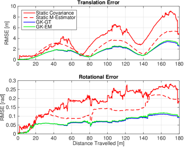
Figure 3: A comparison of translational and rotational Root Mean Square Error on simulated data (RMSE) for four different stereo-visual odometry pipelines: two baseline bundle adjustment procedures with and without a robust Student’s $t$ cost with a fixed and hand-tuned covariance and degrees of freedom (M-Estimation), a robust bundle adjustment with covariances learned from ground truth with algorithm 1 (GK-GT), and a robust bundle adjustment using covariances learned without ground truth using expectation maximization, with algorithm 3 (GK-EM). Note in this experiment, the RMSE curves for GK-GT and GK-EM very nearly overlap. The overall translational and rotational ARMSE values are shown in Table I.

III-B KITTI Dataset

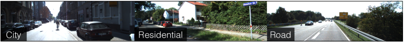
Figure 4: The KITTI dataset contains three different environments. We validate PROBE-GK by training on each type and testing against a baseline stereo visual odometry pipeline.

To evaluate PROBE-GK on real environments, we trained and tested several models on the KITTI Vision Benchmark suite [11, 12], a series of datasets collected by a car outfitted with a number of sensors driven around different parts of Karlsruhe, Germany. Within the dataset, ground truth pose information is provided by a high grade inertial navigation unit which also fuses measurements from differential GPS. Raw data is available for different types of environments through which the car was driving; for our work, we focused on the city, residential and road categories (Figure 4). From each category, we chose two separate trials for training and testing.

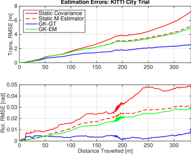
Figure 5: RMSE comparison of stereo odometry estimators evaluated on data from the city category in the KITTI dataset. See Table I for a quantitative summary.

Our prediction space consisted of inertial magnitudes, high and low image frequency coefficients, image entropy, pixel location, and estimated transform parameters. The choice of predictors is motivated by the types of effects we wish to capture (in this case: grassy self-similar textures, as well as shadows, and motion blur). For a more detailed explanation of our choice of prediction space, see our previous work [4].

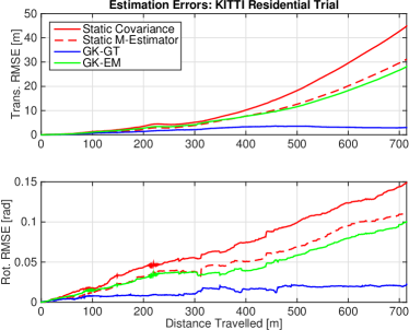
Figure 6: RMSE comparison of stereo odometry estimators evaluated on data from the residential category in the KITTI dataset. See Table I for a quantitative summary.

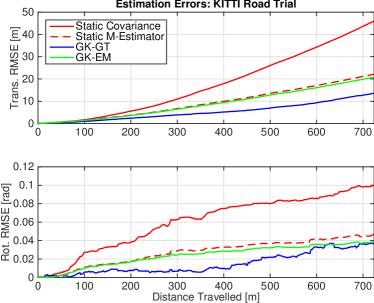
Figure 7: RMSE comparison of stereo odometry estimators evaluated on data from the road category in the KITTI dataset. See Table I for a quantitative summary.

Figures 5, 6 and 7 show typical results; Table I presents a quantitative comparison. PROBE GK-GT produced significant reductions in ARMSE, reducing translational ARMSE by as much as 80%. In contrast, GK-EM showed more modest improvements; this is unlike our synthetic experiments, where both GK-EM and GK-GT achieved similar performance. We are still actively exploring why this is the case; we note that although our simulated data is drawn from a mixture of Gaussian distributions, the underlying noise distribution for real data may be far more complex. With no ground truth, EM has to jointly optimize the camera poses and sensor uncertainty. It is unclear whether this is feasible in the general case with no ground truth information.

Further, we observe that the performance of PROBE-GK depends on the similarity of the training data to the final test trials. A characteristic training dataset was important for consistent improvements on test trials.

III-C Experimental Dataset

TABLE I: Comparison of average root mean squared errors (ARMSE) for rotational and translational components. Each trial is trained and tested from a particular category of raw data from the synthetic and KITTI datasets.

		Trans. ARMSE [m]				Rot. ARMSE [rad]
	Length [m]	Fixed Covar.	Static M-Estimator	GK-GT	GK-EM	Fixed Covar.	Static M-Estimator	GK-GT	GK-EM
Synthetic	180	3.87	2.49	1.59	1.66	0.18	0.13	0.070	0.073
City	332.9	3.84	2.99	1.69	2.87	0.032	0.021	0.0046	0.018
Residential	714.1	13.48	9.37	1.97	8.80	0.068	0.050	0.013	0.044
Road	723.8	17.69	9.38	5.24	8.87	0.060	0.027	0.015	0.024

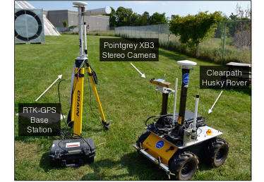
Figure 8: Our experimental apparatus: a Clearpath Husky rover outfitted with a PointGrey XB3 stereo camera and a differential GPS receiver and base station.

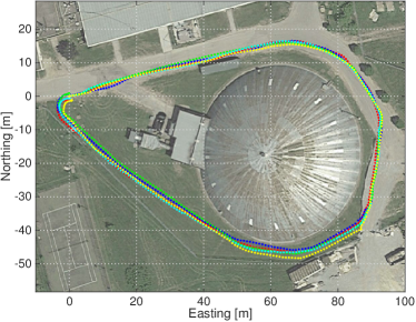
Figure 9: GPS ground truth for 5 experimental trials collected near the UTIAS Mars Dome. Each trial is approximately 250 m long.

To further investigate the capability of our EM approach, we evaluated PROBE-GK on experimental data collected at the University of Toronto Institute for Aerospace Studies (UTIAS). For this experiment, we drove a Clearpath Husky rover outfitted with an Ashtech DG14 Differential GPS, and a PointGrey XB3 stereo camera around the MarsDome (an indoor Mars analog testing environment) at UTIAS (Figure 8) for five trials of a similar path. Each trial was approximately 250 m in length and we made an effort to align the start and end points of each loop. We used the wide baseline (25 cm) of the XB3 stereo camera to record the stereo images. The approximate trajectory for all 5 trials, as recorded by GPS, is shown in Figure 9. Note that the GPS data was not used during training, and only recorded for reference.

For the prediction space in our experiments, we mimicked the KITTI experiments, omitting inertial magnitudes as no inertial data was available. We trained PROBE-GK without ground truth, using the Expectation Maximization approach. Figure 10 shows the likelihood and loop closure error as a function of EM iteration.

The EM approach indeed produced significant error reductions on the training dataset after just a few iterations. Although it was trained with no ground truth information, our PROBE-GK model was used to produce significant reductions in the loop closure errors of the remaining 4 test trials. This reinforced our earlier hypothesis: the EM method works well when the training trajectory more closely resembles the test trials (as was the case in this experiment). Table II lists the statistics for each test.

TABLE II: Comparison of loop closure errors for 4 different experimental trials with and without a learned PROBE-GK-EM model.

		Loop Closure Error [m]
Trial	Path Length [m]	PROBE-GK-EM	Static M-Estimator
2	250.3	3.88	8.07
3	250.5	3.07	6.64
4	205.4	2.81	7.57
5	249.9	2.34	7.75

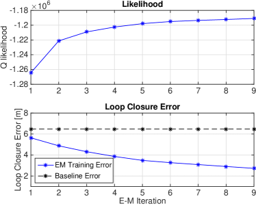
Figure 10: Training without ground truth using PROBE-GK-EM on a 250.2m path around the Mars Dome at UTIAS. The likelihood of the data increases with each iteration, and the loop closure error decreases, improving significantly from a baseline static M-estimator.

IV Related Work

There is a large and growing body of work on the problem of deriving accurate, consistent state estimates from visual data. Although our approach to noise modelling is applicable in other domains, for simplicity we focus our attention on the problem of inferring egomotion from features extracted from sequential pairs of stereo images; see [13] for a survey of techniques. The spectrum of alternative approaches to visual state estimation include monocular techniques, which may be feature-based [14], direct [15], or semi-direct [16].

Apart from simply rejecting outliers, a number of recent approaches attempt to select the optimal set of features to produce an accurate localization estimate from tracked visual features. For example, [17] amend Random Sample Consensus (RANSAC) with statistical hypothesis testing to ensure that tracked visual features have normally distributed residuals before including them in the estimator. Unlike our predictive approach, their technique relies on the availability of feature tracks, and requires scene overlap to work continuously. In a different approach, [18] choose an optimally observable feature subset for a monocular SLAM pipeline by selecting features with the highest informativeness - a measure calculated based on the observability of the SLAM subsystem. Observability, however, is governed by the 3D location of the features, and therefore cannot predict systematic feature degradation due to environmental or sensor-based effects. In contrast, PROBE-GK can leverage prior data to learn such effects and map them to predicted uncertainty on visual observations, optimally weighting the contribution of each observation to the final state estimate.

V Conclusion

The method presented in this paper applies the technique of generalized kernel estimation to improve on the uncorrelated and static Gaussian error models typically employed in stereo odometry. By inferring a more accurate noise model given past sensory experience, we can reduce the tracking error of a sequence of estimates and improve the robustness of our estimator, even when the training data does not have associated ground truth. Our method has the advantage of having relatively few tuning parameters, meaning it can be applied to new problems with very little user intervention. We do rely on the availability of a good set of predictors, and have found that for problems of interest finding a good set is not difficult; a principled choice of an optimal set of predictors, however, remains an interesting open problem.

Although our experiments demonstrate utility only in the context of sequential maximum likelihood estimation on stereo vision data, we believe the model presented here can be applied to a more general class of filter or factor-based estimation algorithms, as well as to a more general class of sensors. In future work, we plan to investigate the applicability of our method to problems of simultaneous localization and mapping, explore the possibility of learning the predictive model online (obviating the need for training data), and examine more principled approaches to selecting an informative prediction space.

References

- [1] M. Fischler and R. Bolles, “Random sample consensus: a paradigm for model fitting with applications to image analysis and automated cartography,” Comm. ACM, vol. 24, no. 6, pp. 381–395, 1981.
- [2] C. Kerl, J. Sturm, and D. Cremers, “Robust odometry estimation for RGB-D cameras,” in Proc. IEEE Int. Conf. Robot. Automat. (ICRA), 2013, pp. 3748–3754.
- [3] P. Agarwal, G. D. Tipaldi, L. Spinello, C. Stachniss, and W. Burgard, “Robust map optimization using dynamic covariance scaling,” in Proc. IEEE Int. Conf. Robot. Automat. (ICRA), 2013, pp. 62–69.
- [4] V. Peretroukhin, L. Clement, M. Giamou, and J. Kelly, “PROBE: Predictive robust estimation for visual-inertial navigation,” in Proc. IEEE/RSJ Int. Conf. Intell. Robots Syst. (IROS), 2015, pp. 3668–3675.
- [5] W. Vega-Brown and N. Roy, “CELLO-EM: Adaptive sensor models without ground truth,” in Proc. IEEE/RSJ Int. Conf. Intell. Robots Syst. (IROS), 2013, pp. 1907–1914.
- [6] T. D. Barfoot and P. T. Furgale, “Associating uncertainty with three-dimensional poses for use in estimation problems,” IEEE Trans. Robot., vol. 30, no. 3, pp. 679–693, 2014.
- [7] A. W. Fitzgibbon, D. P. Robertson, A. Criminisi, S. Ramalingam, and A. Blake, “Learning priors for calibrating families of stereo cameras,” in Proc. IEEE Int. Conf. Computer Vision (ICCV), 2007, pp. 1–8.
- [8] W. R. Vega-Brown, M. Doniec, and N. G. Roy, “Nonparametric bayesian inference on multivariate exponential families,” in Advances in Neural Information Processing Systems 27, 2014, pp. 2546–2554.
- [9] A. Dempster, N. Laird, and D. Rubin, “Maximum likelihood from incomplete data via the EM algorithm,” Journal of the Royal Statistical Society. Series B (Methodological), pp. 1–38, 1977.
- [10] A. Geiger, J. Ziegler, and C. Stiller, “StereoScan: Dense 3D reconstruction in real-time,” in Proc. IEEE Intelligent Vehicles Symp. (IV), June 2011, pp. 963–968.
- [11] A. Geiger, P. Lenz, and R. Urtasun, “Are we ready for autonomous driving? The KITTI vision benchmark suite,” in Proc. IEEE Conf. on Computer Vision and Pattern Recognition (CVPR), 2012.
- [12] A. Geiger, P. Lenz, C. Stiller, and R. Urtasun, “Vision meets robotics: The KITTI dataset,” Int. Journal Robot. Research (IJRR), 2013.
- [13] N. Sünderhauf and P. Protzel, “Stereo odometry: a review of approaches,” Chemnitz University of Technology Technical Report, 2007.
- [14] D. Scaramuzza and F. Fraundorfer, “Visual odometry [tutorial],” IEEE Robot. Automat. Mag., vol. 18, no. 4, pp. 80–92, 2011.
- [15] M. Irani and P. Anandan, “About direct methods,” in Vision Algorithms: Theory and Practice. Springer, 2000, pp. 267–277.
- [16] C. Forster, M. Pizzoli, and D. Scaramuzza, “SVO: Fast semi-direct monocular visual odometry,” in Proc. IEEE Int. Conf. Robot. Automat.(ICRA). IEEE, 2014, pp. 15–22.
- [17] K. Tsotsos, A. Chiuso, and S. Soatto, “Robust inference for visual-inertial sensor fusion,” in Proc. IEEE Int. Conf. Robot. Automat. (ICRA), 2015, pp. 5203–5210.
- [18] G. Zhang and P. Vela, “Optimally observable and minimal cardinality monocular SLAM,” in Proc. IEEE Int. Conf. Robot. Automat. (ICRA), 2015, pp. 5211–5218.