Ordering dynamics of self-propelled particles in an inhomogeneous medium

Abstract

Ordering dynamics of self-propelled particles in an inhomogeneous medium in two-dimensions is studied. We write coarse-grained hydrodynamic equations of motion for density and polarisation fields in the presence of an external random disorder field, which is quenched in time. The strength of inhomogeneity is tuned from zero disorder (clean system) to large disorder. In the clean system, the polarisation field grows algebraically as $L_{\rm P}\sim t^{0.5}$. The density field does not show clean power-law growth; however, it follows $L_{\rm\rho}\sim t^{0.8}$ approximately. In the inhomogeneous system, we find a disorder dependent growth. For both the density and the polarisation, growth slow down with increasing strength of disorder. The polarisation shows a disorder dependent power-law growth $L_{\rm P}(t,\Delta)\sim t^{1/\bar{z}_{\rm P}(\Delta)}$ for intermediate times. At late times, there is a crossover to logarithmic growth $L_{\rm P}(t,\Delta)\sim(\ln t)^{1/\varphi}$, where $\varphi$ is a disorder independent exponent. Two-point correlation functions for the polarisation shows dynamical scaling, but the density does not.

(Accepted in Europhysics Letters)

Collective behaviour of self-propelled particles (SPPs) is observed in a wide variety of systems ranging from micron scales (as in a bacterial colony) to scales of the order of a few kilometers, e.g., animal herds, bird flocks, etc. animalgroup ; helbing ; feder ; kuusela31 ; hubbard ; rauch ; benjacob ; harada ; nedelec ; schaller . Since the seminal work by Vicsek et al. vicsek , collective behaviours of SPPs on homogeneous substrates are studied extensively tonertu ; tonertusr ; srrmp ; vicsekrev ; chatepre ; sppexp . In these studies, the authors characterise different varieties of orientationally ordered steady states in these systems. Recently, work has begun to study the effect of different kinds of inhomogeneity on the steady states of a collection of SPPs disorderst ; bechinger , as inhomogeneity is an inevitable fact of most natural systems.

The study of SPPs is complicated by the fact that the system settles into a non-equilibrium steady state (NESS). There have been very few studies chatepre of the coarsening kinetics from a homogeneous initial state to this asymptotic NESS, though this is of great experimental interest. Previous studies of coarsening or domain growth have primarily focused upon systems approaching an equilibrium state ajbray1994 ; puribook . The ordering dynamics of an assembly of SPPs, both in clean and inhomogeneous environments, is important to understand growth processes in many natural and granular systems. This is the problem we address in the present paper.

The SPPs are defined by their position and orientation (direction of velocity). Each particle moves along its orientation with a constant speed $v_{0}$ and tries to align with its neighbours. In addition to this, we introduce an inhomogeneous random field ${\bf h}$ of fixed strength $\Delta$ and random orientation, but quenched in time. This random field locally aligns the orientation field along a preferred (but random) direction. Such a field may arise from physical inhomogeneities in the substrate, e.g., pinning sites, impurities, obstacles, channels. The random field we introduce here is analogous to the random field in equilibrium spin systems im75 ; tn98 . We write the coarse-grained equations of motion for hydrodynamic variables: density and polarisation. We numerically solve these coupled nonlinear equations for different strengths of disorder. Starting from a random isotropic state, we observe coarsening of the density and the polarisation fields. Our primary focus in this study is the scaling behaviour and growth laws puribook which characterise the emergence of the asymptotic NESS from the disordered state.

Before proceeding, we should stress that there does not as yet exist a clear understanding of the nature of the NESS in the case with substrate inhomogeneity. This problem definitely requires further study. Nevertheless, it is both useful and relevant to study the coarsening kinetics, even without a clear knowledge of the asymptotic state puribook . As a matter of fact, a proper understanding of coarsening kinetics in the inhomogeneous system might also provide valuable information about the corresponding NESS.

In the absence of any inhomogeneity, i.e., in a clean system, the polarisation field grows algebraically with exponent $0.5$, while the density grows with an exponent close to $0.8$. However, the presence of inhomogeneities slows down the growth rate of the hydrodynamic fields in a complicated manner. For intermediate times, domains of the polarisation field follow a power-law growth with a disorder-dependent exponent. At late times, the polarisation field shows a crossover to logarithmic growth, and the logarithmic growth exponent does not depend on the disorder. For large disorder strength, the local polarisation remains pinned in the direction of the quenched random field. However, for the density field, we could not find corresponding unambiguous growth laws.

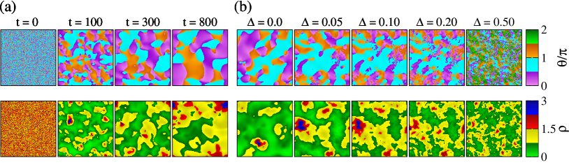
Fig. 1: (colour online) Heat map of (upper panel) the orientation $\theta({\bf r},t)=\tan^{-1}\left({\frac{{\rm P}_{y}({\bf r},t)}{{\rm P}_{x}({\bf r},t)}}\right)$, and (lower panel) the density. (a) shows the evolution of the respective fields with time in the clean system ($\Delta=0$). Starting with random orientation and uniform density at $t=0$, the system coarsens with time. (b) is drawn for different disorder strengths at the same time ($t=1000$). Size of the ordered domains reduces with increasing strength of disorder.

Let us first discuss our model. We consider a collection of SPPs of length $l$, moving on a two-dimensional substrate of friction coefficient $\chi$. Each particle is driven by an internal force $F$ acting along the long axis of the particle. The ratio of the force $F$ to the friction coefficient gives a constant self-propulsion speed $v_{0}=F/\chi$ to each particle. On time-scales large compared to the interaction time, and length scales much larger than the particle size, the dynamics of the system is governed by two hydrodynamic fields: density (which is conserved), and polarisation vector (which is a broken-symmetry variable in the ordered state). The ordered state is also a moving state with mean velocity $v_{0}{\bf P}$. The dynamics of the system is characterised by the coupled equation of motion for the density and polarisation vector. The coarse-grained density equation is

$$\frac{\partial\rho}{\partial t}=-v_{0}\nabla\cdot({\bf P}\rho)+D_{\rho}\nabla^{2}\rho.$$ (1)

The corresponding polarisation equation is

$$\frac{\partial{\bf P}}{\partial t} =[\alpha_{1}(\rho)-\alpha_{2}{\bf P}\cdot{\bf P}]{\bf P}-\frac{v_{0}}{2\rho}\nabla\rho+\lambda_{1}({\bf P}\cdot\nabla){\bf P}$$

$$+\lambda_{2}\nabla(|{\bf P}|^{2})+\lambda_{3}{\bf P}(\nabla\cdot{\bf P})+K\nabla^{2}{\bf P}+{\bf h}.$$ (2)

The hydrodynamic eqs. (1) and (2) are of the same form as proposed on a phenomenological basis by Toner and Tu tonertu to describe the physics of a collection of SPPs. Next we discuss the details of different terms in the above two equations.

In eq. (1), $D_{\rho}$ represents diffusivity in the density field. Since the number of particles is conserved, we can express the R.H.S. of eq. (1) as $-\nabla\cdot{\bf J}$, where the current ${\bf J}$ consists of terms ${\bf J}_{D}\propto\nabla\rho$ and an active current ${\bf J}_{A}\propto v_{0}{\bf P}\rho$. The active current arises because of the self-propelled nature of the particles.

The $\alpha$-terms on the R.H.S. of eq. (2) represent mean-field alignment in the system. For metric distance interaction models, e.g., the Vicsek model, these terms depend on the microscopic model parameters, viz., mean density, noise strength etc. bertinnjop2009 . We choose $\alpha_{1}(\rho)=\frac{\rho}{\rho_{c}}-1$ and $\alpha_{2}=1$. Then the clean system (${\bf h}={\bf 0}$) shows a mean field transition from an isotropic disordered state with ${\rm P}=0$ for mean density $\rho_{0}<\rho_{c}$ to a homogeneous ordered state with ${\rm P}=\sqrt{\frac{\alpha_{1}(\rho_{0})}{\alpha_{2}}}$ for $\rho_{0}>\rho_{c}$. The $\nabla\rho$ term in eq. (2) represents pressure in the system appearing because of density fluctuations. Here, ${\bf P}$ plays a dual role in the SPP system. First, it acts like a polarisation vector order parameter of same symmetry as a two-dimensional $XY$ model. Second, $v_{0}{\bf P}$ is the flock velocity with which the density field is convected. Therefore, we choose same $v_{0}$ for the active current term in the density equation and the pressure term in the polarisation equation, because origin of both is the presence of non-zero self-propelled speed. As soon as we turn off $v_{0}$, the active current turns zero, and the density shows usual diffusive behaviour. Then we can ignore density fluctuations as well as the pressure term. However, in general they can be treated as two independent parameters. $\lambda$ terms are the convective nonlinearities, present because of the absence of the Galilean invariance in the system. $K$ represents diffusivity in the polarisation equation.

To introduce inhomogeneity, i.e., disorder in the system, a random-field term $\mathcal{F}_{h}=-{\bf h}\cdot{\bf P}$ is added in the ‘free energy’. This contributes the term $-\frac{\delta\mathcal{F}_{h}}{\delta\bf P}={\bf h}$ in the polarisation equation. We should stress that such a term coupling to the polarisation field would not arise in the free energy of an equilibrium fluid, but may be realised in the context of the XY model where the polarisation vector is a spin variable. The random field is modeled as ${\bf h}({\bf r})=\Delta\left(\cos\psi({\bf r}),\sin\psi({\bf r})\right)$ where $\Delta$ represents the disorder strength, and $\psi({\bf r})$ is a uniform random angle $\in[0,2\pi]$. We call the model defined by the hydrodynamic eqs. (1) and (2) as a ‘random field active model’ (RFAM). This terminology originates from the well-known random-field Ising model (RFIM), which has received great attention in the literature on disordered systems im75 ; tn98 . We are presently studying the phase diagram of the RFAM. However, a clear determination of this is complicated by the presence of long-lived metastable states. Apart from the RFAM, it is also natural to consider a random-bond active model (RBAM), where the average orientation in the microscopic Vicsek model is weighted with ‘random bonds’ for different neighbours. In this letter, we will focus on the RFAM.

For zero self-propelled speed, i.e., $v_{0}=0$, eq. (1) decouples from the polarisation field and contains only the diffusion current. Hereafter, we refer to this as a ‘zero-SPP model’ (zero-SPPM). In the zero-SPPM, although it contains convective non-linearities, but coupling to density is only diffusive type. For $\Delta=0$, eqs. (1) and (2) reduce to the continuum equations introduced by Toner and Tu tonertu , which represent the clean system. While writing eqs. (1)-(2), all lengths are rescaled by the interaction radius in the underlying microscopic model, and time by the microscopic interaction time. In doing that all the coefficients (speed $v_{0}$, diffusivities $D_{\rho}$, $K$, non-linear coupling $\lambda$’s and field ${\bf h}$) are in dimensionless units. Thus, eqs. (1)-(2) are in dimensionless units.

We should stress that the most general forms of eqs. (1)-(2) also contain noise or “thermal fluctuations”. For domain growth in non-active systems ajbray1994 ; puribook , coarsening kinetics is dominated by a zero-noise (or zero-temperature) fixed point. This is because noise only affects the interfaces between domains, which become irrelevant compared to the divergent domain size po88 . In the present problem, we again have divergent (though different) domain scales for the density and polarisation fields, as we will see shortly. Therefore, it is reasonable to first study the zero-noise versions in eqs. (1)-(2), as we do in the present paper. However, it is also important to undertake a study of the noisy model and confirm the irrelevance of noise.

We numerically solve eqs. (1) and (2) for the hydrodynamic variables. The substrate size is $L\times L$ ($L=256,512,1024,2048$) with periodic boundary conditions in both directions. An isotropic version of Euler’s discretization scheme is used to approximate the partial derivatives appearing in the hydrodynamic equations of motion. In our numerical implementation, the first and second order derivatives for an arbitrary function $f({\bf r},t)$ are discretized as

$$\frac{\partial f}{\partial t} = \frac{f(t+\Delta t)-f(t)}{\Delta t},$$

$$\frac{\partial f}{\partial x} = \frac{f(x+\Delta x)-f(x-\Delta x)}{2\Delta x},$$

$$\frac{\partial^{2}f}{\partial x^{2}} = \frac{f(x+\Delta x)-2f(x)+f(x-\Delta x)}{(\Delta x)^{2}},$$ (3)

where $\Delta t$ and $\Delta x$ are mesh sizes. While solving the equations, the field is specified on each grid point. Thus, we have a field of strength $\Delta$ and random orientation (which is quenched in time) at each grid point. The random angle is chosen from a uniform distribution in the range $[0,2\pi]$. Our numerical scheme is convergent and stable for the chosen grid sizes $\Delta x=1.0$ and $\Delta t=0.1$.

We treat the parameters as phenomenological, and choose $-\lambda_{1}=\lambda_{2}=\lambda_{3}=0.5$, $D_{\rho}=1$, $K=1$ and $v_{0}=0.5$. The above values of $\lambda$’s are chosen for simplicity. We checked that the homogeneous ordered steady state in the clean system is stable shradhapre for the above choice of the parameters, and that can become unstable for large $\lambda$’s. We start with a homogeneous isotropic disordered state with mean density $\rho_{0}=0.75$ and random polarisation, and observe ordering dynamics for different strengths of the random field $\Delta\in[0,1]$. We assume the mean field critical density $\rho_{c}=0.5$ for the clean system.

Fig. 2: (colour online) The main figures show the two-point correlation functions for (a) the polarisation and (b) the density in the clean system ($\Delta=0$), plotted with scaled distances. $C_{\rm P}$ shows good collapse. The insets show plots of correlation function versus distance for the respective fields at different times.

We first study the ordering dynamics of the clean system, i.e., $\Delta=0$. In fig. 1(a), we show snapshots of the orientation (upper panel) $\theta({\bf r},t)=\tan^{-1}\left({\frac{{\rm P}_{y}({\bf r},t)}{{\rm P}_{x}({\bf r},t)}}\right)$, and the density (lower panel) fields at different times. Starting from an initial isotropic state, high density domains with ordered orientation emerge in the system, and the size of these domains increases with time. In the studies of domain growth in far-from equilibrium systems ajbray1994 ; puribook , the standard tool to characterise the evolution of morphologies is the equal-time correlation function $C(r,t)$ of the order-parameter field. We use the same tool for the two fields ${\bf P}({\bf r},t)$ and $\rho({\bf r},t)$, which are relevant in the present context. We introduce the two-point correlation functions:

$$C_{\rm P}(r,t)=\langle{\bf P}({\bf r_{0}},t)\cdot{\bf P}({\bf r_{0}}+{\bf r},t)\rangle_{\bf r_{0}},$$ (4)

and

$$C_{\rm\rho}(r,t)=\langle\delta\rho({\bf r_{0}},t)\delta\rho({\bf r_{0}}+{\bf r},t)\rangle_{\bf r_{0}}.$$ (5)

Here $\delta\rho$ represents fluctuation in the density from its instantaneous local mean value. Angular brackets denote spherical averaging (assuming isotropy), plus an average over space (${\bf r_{0}}$) and over 10 independent runs.

In fig. 2 (a,b) insets, we show the correlation functions $C_{\rm P}$ and $C_{\rm\rho}$ at different times for $\Delta=0$. The data shows coarsening for both the fields, since the correlations increase with time. Characteristic lengths $L_{\rm P}(t,\Delta)$ and $L_{\rm\rho}(t,\Delta)$ are defined as the distance over which the corresponding correlation functions fall to 0.5. In fig. 2(a,b) (main), we plot the correlation functions $C_{\rm P}$ and $C_{\rm\rho}$, respectively, as a function of scaled distance $r/L_{\rm P}$ and $r/L_{\rm\rho}$. We find nice scaling collapse for the polarisation, however, not for the density. Similar results are found for other disorder strengths (data not shown). The absence of dynamical scaling for the density correlation is consistent with the absence of the single energy scale associated with the density growth dynamics ajbray1994 .

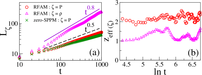
Fig. 3: (colour online) (a) Growth law of the hydrodynamic variables in the clean ($\Delta=0$) system. The self-propelled speed $v_{0}=0.5$ for the random field active model (RFAM), whereas $v_{0}=0$ for the zero-SPP model (zero-SPPM). The straight lines are drawn for the respectively indicated power-laws. (b) Plot of effective growth exponent of the hydrodynamic fields versus time in the clean system for the RFAM.

In fig. 3(a), we show the time dependence of these length scales $L_{\rm\zeta}(t,0)$ where $\zeta\equiv({\bf P},\rho)$. We calculate the growth of the polarisation field for two cases: (i) RFAM with self-propelled speed $v_{0}=0.5$ and (ii) zero-SPPM with $v_{0}=0.0$. For the clean system, we find that the characteristic length follows the similar growth law $L_{\rm P}(t,0)\sim t^{0.5}$ for both the RFAM and the zero-SPPM. The density shows usual diffusive growth for the zero-SPPM (data not shown). Although the data does not show clean power-law for the density, fig. 3(a) shows the growth of the characteristic length as $L_{\rm\rho}(t,0)\sim t^{0.8}$ for the RFAM in the clean system. Faster growth of the density field in our study is consistent with the previous study of self-propelled particles chatepre . We define the algebraic growth law of the hydrodynamic fields in the clean system as $L_{\rm\zeta}(t,0)\sim t^{1/z_{\rm eff(\rm\zeta)}}$, where $z_{\rm eff(\rm\zeta)}$ is the effective growth exponent. In fig. 3(b), we show the variation of the effective growth exponent $z_{\rm eff(\zeta)}$ with time on log-linear scale for the two fields in the RFAM. We find $z_{\rm eff(P)}\sim 2$ for almost two-decades, and $z_{\rm eff(\rho)}\sim 1.2$, when averaged over intermediate and late times, although it shows large oscillations. These oscillations are not due to poor averaging, but rather an intrinsic feature of the density growth in active systems. These may arise due to the absence of a single energy scale for the density growth.

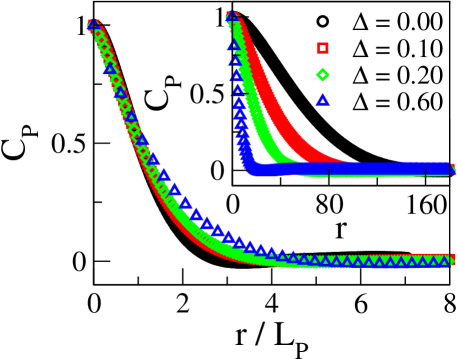
Fig. 4: (colour online) Two-point correlation function for the polarisation, drawn for different disorder strengths. The inset shows $C_{\rm P}$ versus $r$ plot, and the main figure shows scaling collapse of $C_{\rm P}$ as a function of $r/L_{\rm P}$. Morphology of the polarisation field is approximately independent of disorder.

Now we study the effect of disorder in the RFAM. In studies of domain growth, it has been found that random-field and random-bond disorder slows down the coarsening puriepl2017 ; huse1985prl ; lai1988prb ; puriparekh1992 ; paulpurireiger2004 ; purizannetti2011 . This is attributed to the trapping of domain boundaries by sites of quenched disorder puriepl2017 ; huse1985prl ; lai1988prb . As most of the experimental systems contain disorder, here we investigate the effect of random-field disorder on coarsening in the SPPs. In fig. 1(b), we show snapshots of the orientation (upper panel) and the density (lower panel) at time $t=1000$ for different strength of disorder. We find that domain size decreases with increasing $\Delta$. The effect of inhomogeneity in the system is also inferred from the polarisation two-point correlation function shown in fig. 4(inset). Consequently, the characteristic lengths $L_{\rm P,\rho}$ decrease with $\Delta$ as shown in figs. 5(a,b). In fig. 4(main), we plot the two point correlation function $C_{\rm P}$ vs. scaled distance $r/L_{\rm P}$ for fixed time and different strengths of disorder $\Delta=0.0,0.1,0.2$ and $0.6$. We find good scaling collapse of the correlation functions. This suggests that the morphology of the polarisation field is approximately unaffected by disorder. However, this ‘super-universality’ purichowparekh1991 does not extend to the density field which does not even show simple dynamical scaling.

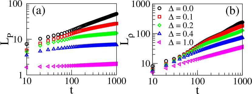
Fig. 5: (colour online) Growth law of the field variables - (a) the polarisation and (b) the density in the RFAM, drawn for different disorder strengths. In the disordered environments, the growth deviates from the power-law at late times.

As stated before for the clean system, $z_{\rm eff(P)}$ shows a mean value $\bar{z}_{\rm P}(\Delta=0)\sim 2$ for an extended range of time. In the RFAM, there is a preasymptotic regime with an effective exponent $\bar{z}_{\rm P}(\Delta)$. As shown in fig. 6(a), $\bar{z}_{\rm P}$ increases with $\Delta$. Also the preasymptotic regime decreases with increasing $\Delta$, and disappears for $\Delta>0.4$. Beyond the mean growth exponent regime, $z_{\rm eff(P)}(t,\Delta)$ increases sharply with time, that signifies pinning of the interfaces because of large disorder strength purizannetti2011 ; equidis .

For the density field, we find $z_{\rm eff(\rho)}(t,0)\sim 1.2$ (not clean power-law). As we increase disorder strength, the effective growth exponent increases, but it does not show a clean power-law and fluctuates very much (data not shown). Hereafter, we characterise the growth law in the presence of disorder for the polarisation field only.

In the presence of disorder, we find a deviation from the power-law growth of the polarisation field. To analyse the effect of disorder, we use the method introduced by Corberi et al. equidis ; purizannetti2011 . They propose the following scaling form for the growth law:

$$L(t,\Delta)\sim t^{1/z_{\rm eff}}=t^{1/{z}}F(\Delta/t^{\phi}).$$ (6)

Here $z_{\rm eff}(t,\Delta)$ represents the effective growth exponent, and $\phi$ is the crossover exponent. The scaling function $F(x)$ behaves as

$$F(x)\sim\begin{cases}\textrm{const.},&\textrm{for }x\rightarrow 0,\\ x^{1/(z\phi)}\textrm{ }\ell\left(x^{-1/\phi}\right),&\textrm{for }x\rightarrow\infty,\end{cases}$$ (7)

where $x=\Delta/t^{\phi}$. For $\phi<0$, scaling form in eq. (6) shows a crossover from the power-law $L\sim t^{1/z}$ to an asymptotic behaviour $L\sim\ell(t\Delta^{1/\lvert\phi\rvert})$. We evaluate the effective growth exponent for the polarisation field using the relation $t=L^{z}G(L/\lambda)$ where the crossover length scale $\lambda=\Delta^{1/\phi z}$, and $G(y)=[F(x)]^{-z}$ with $y=L/\lambda$. Then the effective growth exponent is represented as a function of $y$ as

$$z_{\rm eff}(y)=\frac{\partial\ln t}{\partial\ln L}=z+\frac{\partial\ln G(y)}{\partial\ln y}.$$ (8)

In fig. 6(a), we show the time dependence of $z_{\rm eff(P)}(t,\Delta)$ for $\Delta=0.05,0.1,0.2$ and $0.4$. For the clean system, we find that $z_{\rm eff(P)}$ is close to $2$, as shown in fig. 3(b). For non-zero $\Delta$, the plots show $z_{\rm eff(P)}\simeq\bar{z}_{\rm P}$ for sufficient range of time. $\bar{z}_{\rm P}$ is a disorder-dependent constant. This is followed by late time regime, where $z_{\rm eff(P)}$ is time-dependent. This scenario seems to be a common feature of domain growth in disordered systems as shown in ref. equidis . Hence we can write eqs. (6), (7) and (8) by replacing $z\rightarrow\bar{z}$.

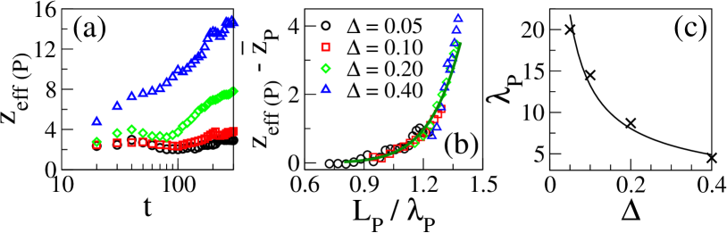
Fig. 6: (colour online) (a) Time variation of the effective growth exponent of the polarisation field in the RFAM, shown for different disorder strengths. (b) The scaling collapse of $z_{\rm eff(P)}-\bar{z}_{\rm P}$ versus $L_{\rm P}/\lambda_{\rm P}$. The best fit $z_{\rm eff(P)}-\bar{z}_{\rm P}\simeq 0.193(L_{\rm P}/\lambda_{\rm P})^{8.86}$ is shown by the solid line. (c) Disorder dependence of $\lambda_{\rm P}$. The solid line shows a power-law fit $\lambda_{\rm P}\sim\Delta^{-0.72}$.

Now we study the dependence of $z_{\rm eff}$ on $L$. From eq. (8), we can say that $z_{\rm eff}-\bar{z}$ only depends on $y=L/\lambda$. In fig. 6(b), we plot $z_{\rm eff(P)}-\bar{z}_{\rm P}$ vs. $L_{\rm P}/\lambda_{\rm P}$ for various disorder values. We choose different $\lambda_{\rm P}$-values for different $\Delta$ to ensure the data collapse. The corresponding values of $\lambda_{\rm P}$ and $\bar{z}_{\rm P}$ for different $\Delta$ are listed in table 1. The solid curve in fig. 6(b) is the best-fit to the power-law form

$$z_{\rm eff}-\bar{z}=by^{\varphi}$$ (9)

with $b=0.193$ and $\varphi=8.86$. In fig. 6(c), we show the $\Delta$ dependence of $\lambda_{\rm P}$, which is fitted by $\lambda_{\rm P}\sim\Delta^{-0.72}$. The negative exponent implies that the disorder is indeed a relevant scaling field. From eq. (9) it is easy to confirm the logarithmic domain growth. The scaling function $G(y)$ can be evaluated by

$$\frac{\partial\ln G(y)}{\partial\ln y}=by^{\varphi}\Rightarrow G(y)\sim\exp\left(\frac{b}{\varphi}y^{\varphi}\right).$$ (10)

Substituting for $G(y)$ in eq. (8) gives the asymptotic logarithmic growth form:

$$\frac{L}{\lambda}\simeq\left[\frac{\varphi}{b}\ln(t/\lambda^{\bar{z}})\right]^{1/\varphi}.$$ (11)

The exponent $\varphi$ has important physical significance in domain-growth studies as it measures how the trapping barriers scale with domain size. In our RFAM, we find $\varphi=8.86$.

Table 1: Parameters $\bar{z}_{\rm P}$ and $\lambda_{\rm P}$ in the RFAM with different $\Delta$ values.

$\Delta$	$0$	$0.05$	$0.10$	$0.20$	$0.40$
$\bar{z}_{\rm P}$	$2.0$	$2.06$	$2.60$	$3.40$	$6.50$
$\lambda_{\rm P}$	$\infty$	$20.0$	$14.50$	$8.70$	$4.50$

In summary, we have studied ordering dynamics in a collection of polar self-propelled particles in an inhomogeneous medium. We use a coarse-grained model, where inhomogeneity is introduced as an external disorder field, which is quenched in time and random in space. The strength of disorder is tuned from $\Delta=0$ to $1.0$ and kept fixed during the evolution of the system.

When the system is quenched from a random isotropic state, both the density and the polarisation fields coarsen with time. In the clean system, i.e., $\Delta=0$, the polarisation field follows the power-law growth $L_{\rm P}(t)\sim t^{0.5}$, while the density field approximately grows as $L_{\rm\rho}(t)\sim t^{0.8}$. We find that the polarisation shows dynamical scaling, whereas the density does not. This indicates that the approach towards the ordered state for the density field is no longer controlled by a single energy scale associated with the cost of a domain wall.

The presence of disorder slows down the growth rate of the hydrodynamic fields. For intermediate time, domains of the polarisation field follow a power-law growth $L_{\rm P}(t,\Delta)\sim t^{1/\bar{z}_{\rm P}(\Delta)}$ with a disorder-dependent exponent $\bar{z}_{\rm P}(\Delta)$. At late times, the polarisation field shows a crossover to logarithmic growth $L_{\rm P}(t,\Delta)\sim(\ln t)^{1/\varphi}$, where the exponent $\varphi$ does not depend on disorder. We find the logarithmic exponent is $\varphi=8.86$ for our two-dimensional RFAM. For large $\Delta$, the local polarisation remains pinned in the direction of the quenched random field. However, we could not find clean growth law for the density field. The scaling function for $C_{\rm P}(r,t)$ is approximately independent of disorder, showing that the morphology of the polarisation field is relatively unaffected by disorder.

In our present study, we find that the disorder plays an important role in the phase ordering dynamics and scaling in a collection of SPPs. Our study provides novel insights on ordering dynamics in a collection of active polar particles in clean as well as disordered environments. The disorder we introduce in our model is analogous to random fields introduced in usual spin systems. It would be interesting to study the effects of other kinds of disorder on ordering dynamics in active systems shradha2014phil ; sdeyprl2012 ; amb2014natcomm .

*****************

R D thanks Manoranjan Kumar for useful discussion regarding the project. S M and S P would like to thank Sriram Ramaswamy for useful discussions at the beginning of the project. S M also thanks S N Bose National Centre for Basic Sciences, Kolkata for kind hospitality (where part of the work is done), and the DST-INDIA (INSPIRE) Research Award for partial financial support.

References

- (1) PARRISH J. K. and HAMNER W. M. (Editors), Animal Groups in Three Dimensions (Cambridge University Press, Cambridge) 1997.
- (2) HELBING D., FARKAS I. J. and VICSEK T., Nature (London), 407 (2000) 487; HELBING D., FARKAS I. J. and VICSEK T., Phys. Rev. Lett., 84 (2000) 1240.
- (3) FEDER T., Phys. Today, 60 (2007) 28; FEARE C., The Starlings (Oxford University Press, Oxford) 1984.
- (4) KUUSELA E., LAHTINEN J. M. and ALA-NISSILA T., Phys. Rev. Lett., 90 (2003) 094502.
- (5) HUBBARD S., BABAK P., SIGUADSSON S. and MAGNUSSON K., Ecol. Modell., 174 (2004) 359.
- (6) RAUCH E., MILLONAS M. and CHIALVO D., Phys. Lett. A, 207 (1995) 185.
- (7) BEN-JACOB E., COHEN I., SHOCHET O., TENENBAUM A., CZIRÓK A. and VICSEK T., Phys. Rev. Lett., 75 (1995) 2899.
- (8) HARADA Y., NOGUSHI A., KISHINO A. and YANAGIDA T., Nature (London), 326 (1987) 805; BADOUAL M., JÜLICHER F. and PROST J., Proc. Nat. Acad. Sci. U.S.A., 99 (2002) 6696.
- (9) NÉDÉLEC F. J., SURREY T., MAGGS A. C. and LEIBLER S., Nature (London), 389 (1997) 305.
- (10) SCHALLER V., WEBER C., SEMMRICH C., FREY E. and BAUSCH A. R., Nature, 467 (2010) 73.
- (11) VICSEK T., CZIRÓK A., BEN-JACOB E., COHEN I. and SHOCHET O., Phys. Rev. Lett., 75 (1995) 1226.
- (12) TONER J. and TU Y., Phys. Rev. Lett., 75 (1995) 4326; TONER J. and TU Y., Phys. Rev. E., 58 (1998) 4858.
- (13) TONER J., TU Y. and RAMASWAMY S., Ann. Phys., 318 (2005) 170.
- (14) MARCHETTI M. C. et al., Rev. Mod. Phys., 85 (2013) 1143.
- (15) VICSEK T. and ZAFEIRIS A., Phys. Rep., 517 (2012) 71.
- (16) CHATÉ H., GINELLI F., GRÉGOIRE G. and RAYNAUD F., Phys. Rev. E, 77 (2008) 046113.
- (17) NARAYAN V., RAMASWAMY S. and MENON N., Science, 317 (2007) 105.
- (18) CHEPIZHKO O., ALTMANN E. G. and PERUANI F., Phys. Rev. Lett., 110 (2013) 238101.
- (19) BECHINGER C., LEONARDO R. D., LÖWEN H., REICHHARDT C., VOLPE G. and VOLPE G., Rev. Mod. Phys., 88 (2016) 045006.
- (20) BRAY A. J., Adv. Phys., 43 (1994) 357.
- (21) PURI S. and WADHAWAN V. K. (Editors), Kinetics of Phase Transitions (CRC Press, Boca Raton) 2009.
- (22) IMRY Y. and MA S.K., Phys. Rev. Lett., 35 (1975) 1399.
- (23) NATTERMANN T., in Spin Glasses and Random Fields, edited by YOUNG A. P. (World Scientific, Singapore) 1998.
- (24) BERTIN E., DROZ M. and GRÉGOIRE G., J. Phys. A: Math. and Theor., 42 (2009) 445001.
- (25) PURI S. and OONO Y., J. Phys. A, 21 (1988) L755.
- (26) MISHRA S., BASKARAN A. and MARCHETTI M. C., Phys. Rev. E, 81 (2010) 061916.
- (27) HUSE D. A. and HENLEY C. L., Phys. Rev. Lett., 54 (1985) 2708.
- (28) LAI Z., MAZENKO G. F. and VALLS O. T., Phys. Rev. B, 37 (1988) 9481.
- (29) KUMAR M., BANERJEE V. and PURI S., EPL, 117 (2017) 10012.
- (30) PURI S. and PAREKH N., J. Phys. A: Math. Gen., 25 (1992) 4127.
- (31) PAUL R., PURI S. and RIEGER H., EPL, 68 (2004) 881.
- (32) CORBERI F., LIPPIELLO E., MUKHERJEE A., PURI S. and ZANNETTI M., J. Stat. Mech: Theo. Exp., (2011) P03016.
- (33) PURI S., CHOWDHURY D. and PAREKH N., J. Phys. A: Math. Gen., 24 (1991) L1087.
- (34) CORBERI F., LIPPIELLO E., MUKHERJEE A., PURI S. and ZANNETTI M., Phys. Rev. E, 85 (2012) 021141.
- (35) MISHRA S., PURI S. and RAMASWAMY S., Phil. Trans. R. Soc. A, 372 (1988) 20130364.
- (36) DEY S., DAS D. and RAJESH R., Phys. Rev. Lett., 108 (2012) 238001.
- (37) WITTKOWSKI R., TIRIBOCCHI A., STENHAMMAR J., ALLEN R. J., MARENDUZZO D. and CATES M. E., Nat. Comm, 5 (2014) 4351.