Target Selection for the SDSS-IV APOGEE-2 Survey

Abstract

APOGEE-2 is a high-resolution, near-infrared spectroscopic survey observing $\sim$3$\times$10⁵ stars across the entire sky. It is the successor to APOGEE and is part of the Sloan Digital Sky Survey IV (SDSS-IV). APOGEE-2 is expanding upon APOGEE’s goals of addressing critical questions of stellar astrophysics, stellar populations, and Galactic chemodynamical evolution using (1) an enhanced set of target types and (2) a second spectrograph at Las Campanas Observatory in Chile. APOGEE-2 is targeting red giant branch (RGB) and red clump (RC) stars, RR Lyrae, low-mass dwarf stars, young stellar objects, and numerous other Milky Way and Local Group sources across the entire sky from both hemispheres. In this paper, we describe the APOGEE-2 observational design, target selection catalogs and algorithms, and the targeting-related documentation included in the SDSS data releases.

1. Introduction

Understanding the parameter space of galaxies, and the processes that drive galaxy evolution, require precise, accurate, multi-wavelength measurements of not only galaxies, but also of their stellar and interstellar building blocks. Photometric and spectroscopic surveys of galaxies can provide global dynamical and chemical properties as a function of redshift, along with spatial variations in these properties down to scales of $\sim$1 kpc for galaxies at $z\sim 0.1$. This is a factor of several larger than the resolution achievable with current MHD simulations of $L_{*}$ galaxies ($\sim$1–50 pc; e.g., Wetzel et al., 2016; Hopkins et al., 2017).

In the Local Group, individual stars can be targeted for spectroscopy in several satellite galaxies, including the Magellanic Clouds, and in the haloes of M31 and M33. But our only access to large numbers of stars in the disk and bulge of a typical $L_{*}$-sized galaxy (where most of the stars in the Universe reside) comes from studies of the Milky Way (MW) Galaxy. A comprehensive understanding of these stellar populations, and the interstellar medium (ISM) between them, provides a critical and unique data point to compare to the end products of cosmological and galactic evolutionary models. This is the advantage of the so-called “near field cosmology”, the use of high-resolution information at very low redshift to constrain the generic physical processes operating at very high redshift.

Surveys of the MW’s stars make up the oldest dedicated astronomical efforts, dating back to Hipparcos and Herschel (1785), among others. Starting in the mid 20th century (shortly after it was proven that the MW was a galaxy; e.g., Curtis, 1917; Hubble, 1926), photometric stellar surveys began to reveal complex structures in the MW, including numerous streams in the halo and the presence of two, seemingly coplanar stellar disks. These surveys have been critically discriminatory datasets used to fuel or reject theories of galaxy formation and evolution. While the basic structure and stellar populations in our Galaxy have been known for this past century, surprises do continue to this day, for example, with the discoveries of the X-shaped bulge in the center (McWilliam & Zoccali, 2010; Nataf et al., 2010; Ness & Lang, 2016) and the presence of multiple stellar populations in globular clusters (e.g., Piotto, 2009; Gratton et al., 2012).

The pace of discovery has been further spurred by the accessibility of long-wavelength optical and infrared (IR) detection technology, which allow photometric and spectroscopic measurements of stars behind the previously-inpenetrable dust in the Galactic disk. These datasets have provided a wealth of both refinements to existing knowledge and new discoveries: for example, the properties of stellar substructure in the outskirts of the disk (with 2MASS; Rocha-Pinto et al., 2003), the existence of a long bar extending 2 kpc beyond the bulge (with GLIMPSE; Benjamin et al., 2005), variations in the IR dust exinction law (with 2MASS and GLIMPSE; Nishiyama et al., 2009; Zasowski et al., 2009), spatially varying peaks in the bulge metallicity distribution (with ARGOS; Ness et al., 2013), and second-generation asymptotic giant branch (AGB) stars and multiple stellar populations in metal-poor and metal-rich bulge globular clusters, respectively (with APOGEE; García-Hernández et al., 2015; Schiavon et al., 2017).

Of course, it is not simply the size or spatial coverage of the observed sample that leads to a deeper understanding of galaxy evolution across cosmic time. Stars occupy a high dimensionality of phase space ($\vec{X}$, $\vec{V}$, [X/H], etc), and mapping their distribution along all of these axes is a key aim of “galactic archeology”, an approach named for its parallels to archeological studies of humans. In both fields, many pieces of complementary evidence from different aspects of a system’s evolution are fitted together into a coherent, multi-layered model. In archeological/historical studies of humans, this may mean combining evidence from tax records, public art, oral histories, and rubbish heaps to understand a complex society’s rise and fall. In galactic archeology, we combine as many dimensions of spatial, dynamical, chemical, and age information as possible to produce a comprehensive model of either a particular galaxy’s evolutionary path, or the full range of evolutionary paths that galaxies can have.

Stellar spectroscopy can access dimensions of stellar phase space largely unreachable by photometry: namely, radial velocities (RVs), precise stellar atmospheric parameters, and metallicity information; at high spectral resolution, individual elemental abundances also become available, which reflect the detailed enrichment history of each star’s natal ISM cloud. When this spectroscopy is performed in the IR on luminous giant stars, these dimensions can be readily obtained for stars throughout the dusty, densely packed inner regions of the MW.

This goal of obtaining high-dimensional stellar information throughout the MW served as the inspiration for the APOGEE survey (Majewski et al., 2017), one of the components of the third generation of the Sloan Digital Sky Survey (SDSS-III; Eisenstein et al., 2011). During 2011–2014, APOGEE obtained high-resolution ($R\sim 22,000$), high SNR, $H$-band spectra for $\sim$163,000 stars in the bulge, disk, and halo of the MW (Zasowski et al., 2013; Holtzman et al., 2015), spanning up to $\sim$12 kpc away in the midplane. Data products publicly released by the survey (Holtzman et al., 2015) include the raw and reduced spectra, radial velocities (Nidever et al., 2015), fundamental stellar parameters (García Pérez et al., 2016; Mészáros et al., 2013; Zamora et al., 2015), and abundances for $\sim$20-25 elements per star (Shetrone et al., 2015; Smith et al., 2013).

The APOGEE-2 survey (Majewski et al., 2016), part of SDSS-IV (2014–2020; Blanton et al., 2017), expands and significantly enhances the original APOGEE sample, with the key addition of a second spectrograph at Las Campanas Observatory (LCO) to make a unqiue all-sky H-band spectroscopic survey. APOGEE-2 thus comprises two complementary components: APOGEE-2 North (APOGEE-2N), using the Sloan Foundation 2.5-meter telescope at APO (Gunn et al., 2006) and original APOGEE spectrograph (Wilson et al., 2012), and APOGEE-2 South (APOGEE-2S), using the duPont 2.5-m telescope at LCO and a cloned spectrograph. The APOGEE-2 sample expands the original red giant sample in both distance and spatial coverage, and further enhancements come from an increasing diversity of targeted objects and scientific goals. The first public release of APOGEE-2 data is contained in Data Release 14 in the summer of 2017 (Abolfathi et al., 2017).

In this paper, we present the target selection and observing strategy of the APOGEE-2 survey. These are critical factors to understand when analyzing data from any survey, to account for selection effects and biases in the base sample (e.g., Schlesinger et al., 2012). In §2, we describe the design of the survey footprint and the organization and prioritization of the targeted objects in each pointing. The logistics of identifying selection criteria applied to individal sample objects is presented in §3. In §4.1, we outline the criteria used to select the primary red giant sample, and §§4.2–4.13 contain information on the numerous other classes of targets, including stellar clusters (§4.2), satellite galaxies (§4.5), and ancillary programs (§4.13). In §5, we describe special calibration targets observed for the purposes of correcting observational artifacts (§5.1) and comparing derived stellar parameters to previous work (§§5.2–5.3). A summary of the targeting information included in the SDSS data releases is presented in §6. A glossary of SDSS- and APOGEE-specific terminology is provided in Appendix A.

2. Field Plan and Observing Strategies

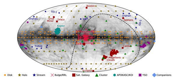
Figure 1.— The current APOGEE-2 field plan in Galactic coordinates, with fields colored by the primary driver of their placement. The background grayscale is the integrated $E(B-V)$ map from Schlegel et al. (1998); the concentration of APOGEE-2 observations in some of the dustiest parts of the Milky Way highlights the targeting advantage of NIR surveys compared to optical ones. The dashed line indicates the approximate declination limit of $-10^{\circ}$ adopted for the Northern (upper, left) and Southern (lower, right) survey components; fields with declinations within $\sim$15^∘ of this line may be observed from either hemisphere. The gray meridians and parallels are spaced every $\Delta l,\Delta b=30^{\circ}$.

2.1. Field Properties

Throughout this paper, we will refer to “fields” or “pointings”, which indicates a patch of sky spanned by a given set or design of targets (§2.3), defined by a central position and radial extent (see below). We will often classify these pointings as “disk fields”, “bulge fields”, “ancillary fields”, etc., which indicates either the dominant MW component in the field or the motivation behind targeting that particular patch of sky. The current APOGEE-2 field plan is shown in Figure 1, with fields colored by type.

The radial extent of a field is driven by the field of view (FOV) of the telescope and the declination of the field itself. The 2.5-m SDSS telescope at APO has a maximal FOV of 1.5^∘ in radius, and the APOGEE instrument on the 2.5-m duPont telescope at LCO has a maximal FOV of 0.95^∘ in radius; these are the maximum design radii of APOGEE-2N and -2S fields, respectively. However, smaller size limits may be imposed on fields observed at high airmass, due to the high differential refraction across the large FOV. Thus, for example, fields with $\delta<-20^{\circ}$ or $\delta>85^{\circ}$ observed from APO have a design radius of $0.9^{\circ}$. At LCO, due to vignetting, we typically impose a limit of 0.8^∘ on survey targets, though exceptions to these rules may exist in special cases.

At the center of each SDSS plate is a hole that blocks targets being placed (e.g., Owen et al., 1994). At APO, plates have a central post that obscures targets within 1.6$\arcmin$, while the use of a central acquisition camera at LCO (which also acts as a post) prevents targets within 5.5$\arcmin$ from the plate center.

The other large class of fields are those in which APOGEE targets are drilled and observed on plates driven by the MaNGA survey of resolved galaxies (Bundy et al., 2015). Because of the MaNGA galaxy selection, these are located towards the Galactic caps, and the APOGEE target selection there is similar to APOGEE-led halo pointings (§4.1). APOGEE does not control the positioning or observing prioritization of these fields. For MaNGA observing details, see Law et al. (2015).

2.2. Field Locations

As in APOGEE-1, fields can be divided into two rough categories: “grid” pointings, which form a semi-regular grid in Galactic longitude and latitude over a particular projected component of the MW, and non-grid pointings, which are placed on particular objects of interest (such as stellar clusters).

The locations of the grid fields in APOGEE-2 are driven by a number of considerations. We note that the separation between Northern and Southern pointings below is largely driven by accessibility and time constraints only; that is, the majority of the total APOGEE-2 field plan, especially the grid pointings, was designed as a coherent strategy to explore the MW, and then divided by hemisphere and slightly modified by time constraints (the North has $\sim$2$\times$ the total amount of observing time as the South). The details of this chronological development of the plan are omitted here, but when considering the motivation for fields that are classified as “North” or “South”, it may be helpful to keep this in mind.

For the Northern program, fields probing the Galactic disk were placed to fill in the APOGEE-1 coverage, or to revisit fields and complete the sample of bright red giants at those locations. Fields in the halo with a faint magnitude limit, the so-called “long” 24-visit fields, are placed on the location of shorter, 3-visit APOGEE-1 fields (Zasowski et al., 2013), to extend the sample at those locations with a larger number of distant stars. Shorter APOGEE-2N halo fields are placed to fill in the grid of short APOGEE-1 halo fields. The few APOGEE-2N bulge fields are dedicated to a pilot study of red clump targets (§4.12).

For the Southern program, we placed fields in the disk and halo to mirror the Northern fields, both APOGEE-1 and -2, as closely as possible. Because of the greater accessibility of the Galactic bulge at LCO, its coverage is significantly expanded than what was achievable from APO. We placed fields in a grid pattern that included revisits to APOGEE-1 pointings and new locations, with a mixture of 1-, 3-, and 6-visit depths. Longer (deeper) fields were placed on key regions of the bulge where larger, fainter samples are expected to be most useful — the bulge/halo interface at $|b|\sim 10^{\circ}$, and along the Galactic major and minor axes, for instance.

Non-grid fields in both hemispheres target stars in particular structures. Fields placed on stellar clusters (§4.2 & 4.7), Kepler or K2 pointings (§4.3–4.4), dwarf galaxies (§4.5), tidal streams (§4.6), or certain ancillary progam targets (§4.13) fall in this category. The exact center of these fields is chosen to include the maximum number of stars of interest, accounting for the FOV of the field (§2.1).

We note that as APOGEE-2 is still ongoing, additional fields may be added before the end of SDSS-IV. For example, because of rapid survey progress enabled by better-than-average weather, program expansions are being considered for the remaining years of bright time at APO. These expansions may include additional fields, or additional observations of existing fields on disk/halo substructures, stellar clusters, or calibration targets, among others. Future publications and the online documentation will describe these changes in detail if they have a significant impact on the targeting strategy or anticipated yields for any part of the APOGEE-2 sample.

2.3. Fields, Cohorts, Designs, Plates

APOGEE-2 targeting employs the same “cohort” strategy adopted in APOGEE-1 to maximize both targeting sample size and magnitude range (Zasowski et al., 2013).

In summary: a “cohort” is a group of stars that are observed together on the exact same visits to their field. Thus, cohorts are selected and grouped based on the number of visits each star is expected to receive; most commonly, this is done by magnitude (e.g., a 12-visit field’s bright targets might only need three visits, but the faintest targets need all 12), but there are exceptions. These exceptions include bright stars being targeted for variability, which would be placed into the longest available cohort (e.g., §4.8) rather than a shorter one with stars of comparable magnitude. For this reason, cohorts are referred to as “short”, “medium”, and “long” — defined by number of visits relative to that of other cohorts in the field — rather than “bright” or “faint”. Which types of cohort are present, and how many visits they correspond to, varies by field.

A “design” is composed of one or more cohorts, and refers to the set of stars (including observational calibration targets: §5.1) observed together in a given visit. A “plate” is the physical piece of aluminum into which holes for all targets in a design are drilled and then plugged with optical fibers leading to the spectrograph. A plate has only one design, but a design can be drilled onto multiple plates. More details can be found in the Glossary in Appendix A, and §2.1 and Figure 1 of Zasowski et al. (2013).

2.4. Design Priorities

The order in which fields are started and completed over the course of the survey depends on a number of factors. For a given night of observing, plates are selected by SDSS scheduling software that takes into account both the plate’s observability at various times of the night and the priority of the plate’s design. For example, if two plates have identical survey priority, but one is observable for one hour that night and the other for three hours, the first one will be chosen for that slot, because the second can be more easily observed later.

The “priority” of a design, as used in this section, is set by the survey. APOGEE-2 has three primary categories of scientific priority for designs: “core”, “goal”, and “ancillary”. The core designs are those that address APOGEE-2’s primary science goals: the bulge, disk, and halo grid pointings (§4.1); stellar clusters (§4.2); a complete astroseismic sample in the original Kepler field (§4.3); satellite galaxies (§4.5); halo stream candidates (§4.6); and red clump and RRL stars in the bulge (§4.9 and §4.12). “Goal” designs are those that use APOGEE-2’s unique capabilities to address related questions: Kepler Objects of Interest (KOIs; §4.4), young star-forming clusters (§4.7), K2 asteroseismic targets (§4.3), and substellar companions (§4.8). There are two other target classes labeled “goal” (M dwarfs and eclipsing binaries, §4.10 and §4.11, respectively), but these targets are sparsely distributed on the sky and appear on designs driven by other factors. Finally, “ancillary” designs are those dominated by ancillary targets (§4.13); small numbers of ancillary targets may also appear on core and goal designs.

These design classifications set a relative priority level in the observation scheduling software, but in practice, observability constraints (including weather) play a greater role in deciding whether a design will be observed or not on any given night. The order in which designs are selected and drilled onto plates, and thus available to be observed, is set by the APOGEE-2 team’s desire for early and ongoing diverse science output. Thus some fields were designed in their entirety early in the survey, and others are gradually designed and observed over the course of several years, in order to both observe a wide range of target types and build large statistical samples within the observing limits of the survey.

The array of fields and targets (and their various stages of completion) that are available in a given data release is a result of all of these factors.

3. Targeting Flags

Understanding how representative APOGEE-2’s spectroscopic target sample is of the stellar populations in the survey footprint requires knowing how that sample was selected from the underlying population. APOGEE-2 uses three 32-bit integers (“targeting flags”, composed of “targeting bits”) to encode the criteria that are used to select targets. Every target in a given design is assigned one of each of these integers, whose bits indicate which criteria were applied to select that particular target for that particular design (e.g., color limit, calibration target, ancillary program). Thus each target may have up to 96 bits of targeting information associated with it (currently, not all bits are in use). These targeting flags are design-specific, because targets can be selected for different reasons in different designs covering the same spatial location. In practice, this situation is rare, but we note the possibility for completeness.

As in APOGEE-1 and the online documentation, throughout this paper we will use the shorthand notation “${\rm APOGEE2\_TARGET}X={\rm A}$” to indicate that the targeting flag APOGEE2_TARGETX has targeting bit A set. Technically, this bit is set by adding $2^{\rm A}$ to the targeting flag. Frequently, targets will have multiple bits set, and their final targeting flags are sums of these bits:

$${\rm APOGEE2\_TARGET}X=\sum_{i=0}^{N}{2^{{\rm bit}(i)}}.$$ (1)

A list of APOGEE-2’s current targeting bits is given in Table 1. Targets observed during APOGEE-1 use the APOGEE_TARGETX flags (note the difference between APOGEE_$\ast$ and APOGEE2_$\ast$); see the SDSS DR12 documentation and Table 1 of Zasowski et al. (2013) for these definitions.

For example, a star that is chosen as a calibration cluster member (§4.2) that was also observed in APOGEE-1 (§5.3) would have ${\rm APOGEE2\_TARGET2=10}$ and ${\rm APOGEE2\_TARGET2=6}$ set; if this star also happens to have been simultaneously selected as a member of the random red giant sample (§4.1), it will have the associated dereddening method and cohort color and magnitude limit bits set as well. See the DR14 SDSS bitmask documentation and APOGEE-2 targeting documentation for examples of targeting bit usage.

Finally, we note that these are targeting flags — they indicate why a particular object was selected for spectroscopic observation. They do not indicate the actual nature of the object or include any information learned from those observations. For example, stars targeted as possible members of open clusters may turn out not be actual members, and stars not targeted (and flagged) as possible members may in fact be members. The targeting flags should be used to reconstruct the survey selection functions and identify targets associated with certain programs (such as ancillary projects), not to identify a comprehensive list of particular types of objects.

Table 1APOGEE-2 Targeting Bits

APOGEE2_TARGET1		APOGEE2_TARGET2		APOGEE2_TARGET3
Bit	Criterion	Bit	Criterion	Bit	Criterion
0	Single $(J-K_{s})_{0}>0.5$ bin	0	—	0	KOI target
1	“Blue” $0.5<(J-K_{s})_{0}<0.8$ bin	1	—	1	Eclipsing binary
2	“Red” $(J-K_{s})_{0}>0.8$ bin	2	Abundance/parameters standard	2	KOI control target
3	Dereddened with RJCE/IRAC	3	RV standard	3	M dwarf
4	Dereddened with RJCE/WISE	4	Sky fiber	4	Substellar companion search target
5	Dereddened with SFD $E(B-V)$	5	External survey calibration	5	Young cluster target
6	No dereddening	6	Internal survey calibration (APOGEE-1+2)	6	—
7	Washington+DDO51 giant	7	—	7	—
8	Washington+DDO51 dwarf	8	—	8	Ancillary target
9	Probable (open) cluster member	9	Telluric calibrator	9	—
10	—	10	Calibration cluster member	10	– QSOs
11	Short cohort (1–3 visits)	11	—	11	– Cepheids
12	Medium cohort (3–6 visits)	12	—	12	– The Distant Disk
13	Long cohort (12–24 visits)	13	Literature calibration	13	– Emission Line Stars
14	Random sample member	14	Gaia-ESO overlap	14	– Moving Groups
15	MaNGA-led design	15	ARGOS overlap	15	– NGC 6791 Populations
16	Single $(J-K_{s})_{0}>0.3$ bin	16	Gaia overlap	16	– Cannon Calibrators
17	No Washington+DDO51 classification	17	GALAH overlap	17	– Faint APOKASC Giants
18	Confirmed tidal stream member	18	RAVE overlap	18	– W3-4-5 Star Forming Regions
19	Potential tidal stream member	19	APOGEE-2S commissioning target	19	– Massive Evolved Stars
20	Confirmed dSph member (non Sgr)	20	—	20	– Extinction Law
21	Potential dSph member (non Sgr)	21	—	21	– Kepler M Dwarfs
22	Confirmed Mag Cloud member	22	1-m target	22	– AGB Stars
23	Potential Mag Cloud member	23	Modified bright limit cohort ($H<10$)	23	– M33 Clusters
24	RR Lyra star	24	Carnegie (CIS) program target	24	– Ultracool Dwarfs
25	Potential bulge RC star	25	Chilean (CNTAC) community target	25	– SEGUE Giants
26	Sgr dSph member	26	Proprietary program target	26	– Cepheids
27	APOKASC “giant” sample	27	—	27	– Kapteyn Field SA57
28	APOKASC “dwarf” sample	28	—	28	– K2 M Dwarfs
29	“Faint” target	29	—	29	– RV Variables
30	APOKASC sample	30	—	30	– M31 Disk

4. Science Sample Target Selection

4.1. Main Red Giant Sample

The targeting strategy for the primary red giant sample is very similar to that in APOGEE-1. We begin with the 2 Micron All Sky Survey Point Source Catalog (2MASS PSC; Skrutskie et al., 2006) and add mid-IR photometry from the Spitzer-IRAC GLIMPSE (Benjamin et al., 2005; Churchwell et al., 2009) and AllWISE (Wright et al., 2010; Cutri et al., 2013) catalogs. After applying data quality limits to ensure reliable photometry (Table 2), we use the RJCE method to calculate dereddened $(J-K_{s})_{0}$ colors (Majewski et al., 2011). In some cases, particularly in the low-extinction halo fields, integrated $E(B-V)$ values from the Schlegel et al. (1998, hereafter SFD) maps are used for dereddening instead of the RJCE values. The method used for each target is stored in that object’s targeting flags (§3).

Table 2Main Red Giant Sample Data Quality Requirements

Parameter	Requirement
2MASS total photometric uncertainty for $J$, $H$, and $K_{s}$	$\leq$0.1
2MASS quality flag for $J$, $H$, and $K_{s}$	$=$“A” or “B”
Distance to nearest 2MASS PSC source	$\geq$6′′
2MASS confusion flag for $J$, $H$, and $K_{s}$	$=$“0”
2MASS galaxy contamination flag	$=$“0”
2MASS read flag	$=$“1” or “2”
2MASS extkey ID	$=$Null
Photometric uncertainty for IRAC [4.5$\mu$m]	$\leq$0.1
Photometric uncertainty for WISE [4.6$\mu$m]	$\leq$0.1
chi for $M$, $T_{2}$, and DDO51 data	$<$3
$|$sharp$|$ for $M$, $T_{2}$, and DDO51 data	$<$1

Stellar cohorts in the disk, bulge, and some halo fields are selected from candidate pools defined by ranges of $(J-K_{s})_{0}$ color and $H$ magnitude. Bulge and halo field cohorts use a single color limit of $(J-K_{s})_{0}\geq 0.5$ and $(J-K_{s})_{0}\geq 0.3$, respectively. MaNGA-led fields, which lie towards the Galactic halo, are treated like halo fields in this respect.

In a departure from APOGEE-1, the APOGEE-2 disk fields utilize a two-color-bin scheme, with $N_{\rm blue}$ stars drawn from $0.5\leq(J-K_{s})_{0}\leq 0.8$, and $N_{\rm red}$ stars drawn from $(J-K_{s})_{0}\geq 0.8$. This scheme is designed to increase the fraction of distant red giant stars. The ratio between $N_{\rm blue}$ and $N_{\rm red}$ is set by the disk field’s longitude: if the central longitude is $<120^{\circ}$ or $>240^{\circ}$, then half of that cohort’s fibers are drawn from each bin (i.e., $N_{\rm blue}=N_{\rm red}$). For outer disk fields with $120^{\circ}\leq l\leq 240^{\circ}$, the blue bin contains 25% of the cohort fibers, and the red bin contains 75%. Figure 2 illustrates these selection bins for one of the disk fields. If there aren’t enough stars available in a color bin, the “extra” fibers are assigned targets drawn from the other bin.

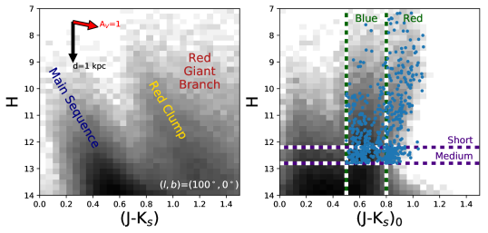
Figure 2.— RJCE dereddening and target selection in the 6-visit disk field 100+00. The left panel shows the observed $(J-K_{s},H)$ CMD, with the primary populations labeled. The right panel contains the same stars in the dereddened $([J-K_{s}]_{0},H)$ CMD, overplotted with this field’s targets (blue points). As described in §4.1, targets are drawn from multiple bins in $H$ magnitude and dereddened $(J-K_{s})_{0}$ color.

The faint magnitude limit of a cohort is set by the anticipated number of visits to that cohort, such that the faintest stars achieve the target summed S/N of 100 per pixel (see Table 3). For Northern cohorts, these faint limits are identical to APOGEE-1. The bright limit is set by the faint limit of shorter cohorts in the design, or by $H>7$ (the approximate saturation limit for a single visit) for the shortest cohort. For some disk fields, a fainter bright limit of $H>10$ is adopted to avoid very nearby stars; targets in these designs have targeting bit APOGEE2_TARGET2=23 set. All of the designs in MaNGA-led fields were anticipated to be 3-visit cohorts, but with a slightly brighter faint limit of $H<11.5$ to account for flux loss due to MaNGA’s arcsec-sized spatial dither pattern (Table 3).

Table 3Typical $H$ Magnitude Limits of Primary APOGEE Cohorts

$N_{\rm visits}$	$H_{\rm min}-H_{\rm max}$
1	7.0–11.0
3	7.0–12.2
6	7.0–12.8 or 12.2–12.8
12	12.8–13.3
24	13.3–13.8

Furthermore, a number of the Northern halo fields have additional target selection and prioritization based on stellar colors in the Washington $M$ & $T_{2}$ and DDO51 filters (hereafter “W+D photometry”). This technique takes advantage of the fact that because of the gravity sensitivity of the DDO51 filter, dwarf and giant stars form distinct loci in the $(M-T_{2})$ vs. $(M-DDO51)$ color-color plane over a wide range of stellar temperature (e.g., Majewski et al., 2000). The application of this technique to select and prioritize giant stars in APOGEE targeting is described in §4.2 of Zasowski et al. (2013), and APOGEE-2 uses the same classification method and subsequent observing priorities. That is, when selecting stars for a cohort with given color and magnitude limits, stars classified as “giants” based on their W+D photometry are chosen first; if any fibers allocated to that cohort remain, stars without W+D photometric classifications are chosen next, followed by those classified as “dwarfs.”

Proper motions for the APOGEE-2 main sample stars are drawn from the URAT1 catalog (Zacharias et al., 2015) and used to correct the target positions to the proper epoch before drilling the plates. No proper motion data are used in the selection or prioritization of main sample targets. APOGEE-2 observations later in the survey may use other proper motion catalogs, as improved ones become available (e.g., Gaia and UCAC5; Gaia Collaboration et al., 2016a; Zacharias et al., 2017).

We emphasize that the color, magnitude, and W+D photometric criteria described here apply to stars selected as part of the primary red giant sample only. This component comprised $\sim$2/3 of the total APOGEE-1 sample, and we anticipate a similar fraction of the total APOGEE-2 sample. The exact final proportion of main-sample red giant stars will depend on, e.g., the presence of additional ancillary programs, re-allocation of bright time made available by rapid observing progress, or other survey improvements. Users of the main sample data should always check the documentation for the relevant data release for any updates to these criteria. The subsections below describe the selection procedures for other components of the APOGEE-2 survey.

4.2. Open and Globular Clusters

Stellar clusters are valuable targets for chemical or dynamical surveys of the MW. They provide a large number of stars with nearly identical ages, distances, and velocities, which can thus be measured more accurately and precisely than for isolated field stars. Despite this, globular clusters are known to generally host multiple stellar populations (e.g., Milone et al., 2017), with well-characterized patterns in certain elemental abundances (see Gratton et al., 2012, for a review). In contrast, open clusters are generally considered to represent single populations with internally consistent abundances (e.g., Bovy, 2016; Ness et al., 2017, but see also Liu et al. (2016a, b)). Together, clusters represent star formation histories in a range of mass, metallicity, and Galactic environment.

Globular clusters in particular have been extensively studied with both photometry and spectroscopy, and this wealth of dynamical and chemical literature provides valuable benchmarks to calibrate newly derived datasets onto existing scales. In addition, because clusters have little internal spread in age and (generally) in [Fe/H], their RGBs are useful for calibrating the behavior of $T_{\rm eff}$ and $\log{g}$ at fixed abundance.

For all of these reasons, open and globular clusters are targeted by APOGEE-2 for both scientific analysis and calibration. APOGEE-1 observed a benchmark set of the globular clusters, and many of the open clusters, accessible in the Northern Hemisphere (see Mészáros et al., 2013; Holtzman et al., 2015, for calibration details). In APOGEE-2, we revisit some Northern globular clusters (including M5, PAL 5, M12, M15, and M71) to increase the number of observed members. In addition, the circumpolar open cluster NGC 188 is periodically observed from the North to monitor any long-term changes in the survey data properties, and other systems (including the open cluster NGC 2243) are observed with both the Northern and Southern instruments for internal cross-calibration (§5.3).

APOGEE-2S is targeting a large number of globular and open clusters that are inaccessible to APOGEE-1 and APOGEE-2N. Dedicated survey fields are placed on well-studied globular clusters with substantial pre-existing literature parameters, listed in Table 4, and another $\sim$10 globular clusters located towards the inner Galaxy fall at least partially within planned APOGEE-2S disk or bulge survey fields. Targets in these clusters are selected and prioritized using a combination of pre-existing information and observing constraints imposed by APOGEE-2S’s magnitude and fiber collision limits. As in APOGEE-1, targeted members are selected according to the following priorities:

1. presence of stellar atmospheric parameters and/or abundances derived from high-resolution data,

2. RV membership,

3. proper motion membership, and

4. location in the color-magnitude diagram (CMD), guided by the CMD locus of known members according to the previous criteria.

Figure 3 shows the targets chosen with these selection categories for the globular cluster NGC 6752.

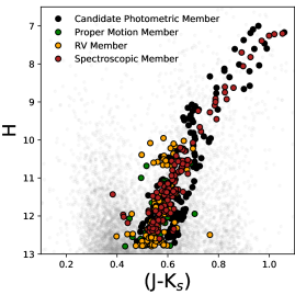
Figure 3.— CMD of targets in the globular cluster NGC 6752 and their priority classes, from stars with 2MASS colors consistent with the cluster locus (lowest priority, black circles), through known members with previous spectroscopic information (highest priority, red circles). The faint gray points in the background are the rest of the 2MASS sources in the field that were not targeted as part of the cluster selection.

These targets are then sorted into cohorts (§2.3) to maximize the sample size by eliminating fiber colllisions. Additional fibers are filled with cluster members (according to the above criteria) fainter than the nominal magnitude limit for the field or with field stars selected as part of the main survey’s red giant sample (§4.1). Stars selected as calibration cluster members (based on literature spectroscopic parameters and/or proper motion or RV membership probabilities) have the targeting bit APOGEE2_TARGET2=10 set, and stars selected because they have high quality literature parameters or abundances have bit APOGEE2_TARGET2=2 set. Note that these two flags are not mutually exclusive.

Open clusters without significant literature of individual members are generally targeted using the selection algorithm described in Frinchaboy et al. (2013). In summary, this is a spatial and photometric selection that uses information from the stellar sky positions, line-of-sight reddening, and proximity to a cluster isochrone derived from previous work (if known) to identify the likeliest cluster members. Stars selected as potential open cluster members have the targeting bit APOGEE2_TARGET1=9 set. Analysis of APOGEE-1’s open clusters began with Frinchaboy et al. (2013) and Cunha et al. (2016), and APOGEE-2 South is extending this large, homogeneous sample with $\gtrsim$100 clusters in the rich star formation regions of the southern Galactic disk.

Table 4Observed and Anticipated Calibration Clusters

Cluster Name	NGC ID	[Fe/H]	Distance (kpc)	APOGEE-2 Field
M5	NGC 5904	$-1.33\pm 0.02$	7.5	M5PAL5
47Tuc	NGC 104	$-0.76\pm 0.02$	4.5	47TUC
	NGC 288	$-1.32\pm 0.02$	8.9	N288
	NGC 362	$-1.30\pm 0.04$	8.6	N362
	NGC 1851	$-1.18\pm 0.08$	12.1	N1851
M79	NGC 1904	$-1.58\pm 0.02$	12.9	M79
	NGC 2808	$-1.28\pm 0.04$	9.6	N2808
	NGC 3201	$-1.51\pm 0.02$	4.9	N3201
M68	NGC 4590	$-2.27\pm 0.04$	10.3	M68
$\omega$ Cen	NGC 5139	$-1.64\pm 0.09$	5.2	OMEGACEN
M4	NGC 6121	$-1.18\pm 0.02$	2.2	M4
M12	NGC 6218	$-1.33\pm 0.02$	4.8	M12
M10	NGC 6254	$-1.57\pm 0.02$	4.4	M10
	NGC 6388	$-0.45\pm 0.04$	9.9	N6388
	NGC 6397	$-1.99\pm 0.02$	2.3	N6397
	NGC 6441	$-0.44\pm 0.07$	11.6	N6441
M22	NGC 6656	$-1.70\pm 0.08$	3.2	M22
	NGC 6752	$-1.55\pm 0.01$	4.0	N6752
M55	NGC 6809	$-1.93\pm 0.02$	5.4	M55

4.3. Asteroseismic Targets

Precise, high-cadence time-series photometry and spectroscopy of stars reveals that the surfaces of even non-variable, seemingly inactive stars fluctuate in response to standing waves reverberating throughout the star’s layers. Just as in Earth-based seismology, these wave patterns are affected by the density of the layers they encounter. Through the analysis of these “solar-like oscillations” in a star, the fundamental stellar parameters of mass and radius (thus surface gravity) can be determined with high precision; when combined with spectroscopic temperature and abundance measurements, the age of a typical red giant star can be determined with $\sim$30% accuracy. This combination of data also provides masses for stars of known $T_{\rm eff}$ and abundance, rotation-based ages for dwarf stars via gyrochronological relationships, and diagnostics of internal stellar structure and pulsation mechanisms.

Highly precise, asteroseismic measurements of fundamental stellar parameters are valuable calibrators for less precise spectroscopic measurements, and benchmarks for models of stellar interiors and stellar atmospheres. Stars with both asteroseismic and spectroscopic data are very useful for addressing numerous Galactic astrophysical questions, including the chemical and dynamical evolution of stellar populations and the demographics of transiting exoplanet host stars. In APOGEE-1, targets from two space satellites with asteroseismic data were observed. Anders et al. (2017) describes the APOGEE observations of $\sim$600 red giants with asteroseismic data from the CoRoT satellite (Baglin et al., 2006). The APOGEE-Kepler Asteroseismic Science Consortium sample (APOKASC sample; Pinsonneault et al., 2014) includes more than 6000 giant and 400 dwarf stars with measured asteroseismic properties from the Kepler satellite (Borucki et al., 2010).

The initial APOKASC sample came from Kepler’s original pointing in Cygnus. The bulk of the stars were selected based on their brightness, their photometric temperature, and the detection of solar-like oscillations in their light curves. (For details of the rest of the Cygnus APOKASC targets, see §8.3 in Zasowski et al., 2013).

The APOGEE-2 APOKASC program is expanding this selection to build a magnitude-limited sample of Kepler stars, which contains significant improvements over the earlier subset. In APOGEE-1, potential targets meeting the selection criteria were prioritized in ways that bias towards certain kinds of stars (e.g., first ascent RGB stars were preferred over RC stars), and the selection criteria themselves eliminated interesting stars (e.g., RGB stars without solar-like oscillations). In addition, the stellar parameter spece spanned by the initial APOKASC catalog is relatively sparsely sampled.

These limitations were unavoidable, given APOKASC’s available time in APOGEE-1, and APOGEE-2 is dedicating a large amount of observing time to overcome them. In the original Cygnus field, the remaining $\sim$13,500 cool stars with $7\leq H\leq 11$ not yet observed with APOGEE are targeted, regardless of evolutionary state or the presence of oscillations. Giants are identified using $T_{\rm eff}<5500$ K and $\log{g}<3.5$, and dwarfs with $5000\leq T_{\rm eff}\leq 6500$ K and $\log{g}>3.5$; pre-observation temperature and gravity estimates come from the revised Kepler Input Catalog (Huber et al., 2014) and the corrected temperature scale of Pinsonneault et al. (2012). These targets are distributed across the same 21 fields used in APOGEE-1 APOKASC, and are observed with a total of $\sim$50 single-visit designs.

In 2013, the second of the Kepler spacecraft’s four reaction wheels failed, leaving the satellite unable to remain stably pointed at the Cygnus field. The telescope was then repurposed for the K2 mission, performing very similar observations at numerous pointings along the ecliptic plane in 75-day intervals (Howell et al., 2014). Though stellar asteroseismic measurements from these data are noisier than their counterparts from the $\sim$4 year Kepler-Cygnus data, the K2 sample is highly valuable for Galactic stellar and planetary studies because it includes stars spanning an enormous range of Galactic environment, from stellar clusters and the halo to the bulge.

APOGEE-2 is targeting more than 10⁴ giant stars in several of these K2 pointings (called “campaigns”), mostly from the K2 Galactic Archaeology Program’s (GAP) sample of asteroseismic targets. These stars are selected from the pool of GAP candidates based purely on the their magnitude, with additional non-GAP stars selected as oscillators based on K2 data. The total sample is observed over at least 50 visits divided amongst the campaigns, all or nearly all of which are being observed from the North.

All APOKASC targets have targeting bit APOGEE2_TARGET1=30 set, with giants and dwarfs being further identified with APOGEE2_TARGET1=27 and 28, respectively, if applicable.

4.4. Kepler Objects of Interest

The Kepler satellite has identified thousands of transiting planets confirmed through follow-up spectroscopy or imaging. Prior to confirmation, a star with transit signals potentially consistent with orbiting planets is called a “Kepler Object of Interest” (KOI). As a class, KOIs include genuine planet hosts along with eclipsing binary systems, brown dwarf hosts, strongly spotted stars, and other systems with light curves that can masquerade as transiting planet signatures.

High-resolution, high-cadence spectroscopy can distinguish many of the “false positive” cases from true planets (Fleming et al., 2015). While the APOGEE RV precision is generally insufficient to detect planets directly, the data can identify several of the most common classes of false positives, including eclipsing binaries with grazing orbits, tertiary companions diluting binary system eclipse depths, and very low mass stars or brown dwarfs, with radii (and thus transit depths) similar to those of gas giant exoplanets but with much larger masses. The RV signal of these types of systems ranges from several hundred m s^-1 to tens of km s^-1. Using the Kepler planet sample to improve our understanding of planetary system formation and stellar host demographics requires 1) using multi-epoch RV data to strictly constrain the false positive rate as a function of stellar type, and 2) measuring the stellar properties of both planet-hosting and non-planet-hosting populations with significant statistics (see also §4.8).

APOGEE-2 is making observations to address both of these requirements, using samples of confirmed planet hosts, KOIs, and non-hosts in the Kepler Cygnus footprint. The primary goal is to homogeneously measure the binary fraction, chemical compositions, and rotational velocities for significant samples of both KOIs and non-KOIs. The first two properties are thought to have an impact on planet frequency and habitability, and the third can be used to constrain stellar activity and tidal effects, which also affect planetary system properties. Furthermore, the spectroscopic RVs and rotational velocities can help discriminate among different sources of false positives to provide a cleaner planet sample, and some of these sources (such as brown dwarfs) are scientifically interesting objects in their own right.

The APOGEE-2 KOI program contains $\sim$1000 KOIs and $\sim$200 non-hosts distributed across five APOGEE-2 fields, supplemented by $\sim$200 KOIs observed in APOGEE-1. Planet hosts and KOIs were drawn from the NExScI archive using a simple magnitude limit of $H<14$ to identify all CONFIRMED or CANDIDATE targets in the fields. The non-host “control sample” was drawn from the Kepler Input Catalog (Brown et al., 2011), using the same $H<14$ magnitude limit and selected to provide the same $T_{\rm eff}$–$\log{g}$ joint density distribution as in the host+KOI sample. These control sample stars are used to fill fibers unused by the host+KOI sample.

Each APOGEE-2 KOI field is observed over 18 epochs, with cadencing sufficient to characterize a wide range of orbits. The host+KOI targets can be identified with the targeting bit APOGEE2_TARGET3=0, and the control sample targets with APOGEE2_TARGET3=2.

4.5. Satellite Galaxies

The bulk of the APOGEE-2 programs are dedicated to measuring chemo-dynamical properties of stars within the MW. However, placing these properties in the context of the MW’s evolution, and of galaxy evolution in general, requires comparable measurements of other stars in the Local Group. APOGEE-2 is targeting stars in eight Local Group satellite galaxies: the Large and Small Magellanic Clouds (LMC, SMC; §4.5.1) and six dwarf spheroidal galaxies (dSphs; §4.5.2).

4.5.1 Magellanic Clouds

The LMC and SMC are the two most massive satellite galaxies of the MW, and at distances of only $\sim$50 kpc and $\sim$60 kpc, respectively, they span angles on the sky large enough for APOGEE to obtain velocity and chemical information for thousands of individual stars. By mapping the kinematics and abundances of these stars, as well as the interplay between stellar and gas kinematics, across the galaxies and the MW, we can explore the mass dependence of chemical evolution and feedback in the range of $10^{8}-10^{10}~{}M_{\sun}$.

APOGEE-2 is targeting $\sim$3500 stars in $\sim$17 fields spanning the LMC down to a magnitude limit of $H=14.6$, and $\sim$2000 stars in $\sim$9 fields in the SMC down to $H=14.9$; two of the SMC fields include the MW globular clusters 47 Tuc and NGC 362. The LMC fields extend from the center of the LMC out to $\sim$9.5^∘ along the major axis and $\sim$6.5^∘ on the minor axis; the SMC fields span up to $\sim$5^∘ away from the SMC’s center along both axes. These fields cover approximately 1/3 of the sky area within those ranges. Their exact placement is driven by the desire for well-sampled radial and azimuthal coverage, as well as for a high local density of MC RGB stars and the presence of DES or SMASH photometry (Dark Energy Survey Collaboration et al., 2016; Nidever et al., 2017), which can provide star formation histories for the spectroscopic sample.

The MC targets comprise four primary types of stars: RGB stars, AGB stars, young massive stars, and other rare massive evolved stars (Figure 4). RGB stars provide a dense sampling of the abundance gradients and chemical evolution of the MCs, including in the poorly understood SMC and outer regions of the LMC. These outer pointings will also be used to look for tidal streams and other substructures in these low mass halos, which are predicted by hierarchical formation models; one such stream has already been detected (Olsen et al., 2011), and APOGEE’s numerous chemical abundances will be powerful tools for identifying others.

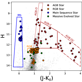
Figure 4.— CMD of targets and target classes in a sample LMC field (LMC-9). Red points indicate AGB stars, comprising AGB-O, AGB-C, and dusty AGB-C (AGB-DC) stars appearing in three different color-magnitude bins. Orange indicates RGB stars, which include both stars selected from the orange box and those with existing literature data. Blue are hot main sequence stars, selected from the drawn box, and green are other massive evolved stars selected from the literature. Gray points are other 2MASS sources in the field that were not targeted as LMC stars.

AGB stars, though poor probes of galactic chemical evolution because of the internal mixing that has modified their atmospheric abundances, are important tracers of stellar chemical evolution for the same reason. Measurement of abundances that are expected to be altered by physical processes and AGB nucleosynthesis, compared to abundances of the less-evolved RGB stars, enable studies of the mass- and metallicity-dependence of processes such as third dredge-up, hot bottom burning, and the synthesis of elements such as N, C, Na, Al, and Mg (e.g., Ventura et al., 2015, 2016). At the other end of the stellar lifecycle, young hot stars in the MCs contain chemodynamical information from very recent and ongoing star formation, to compare with co-spatial gas measurements and with the more evolved stellar populations.

APOGEE-2 targeting in the LMC and SMC uses extensive photometric and spectroscopic information to produce a large, clean set of diverse targets. Candidate stellar targets in LMC and SMC fields are divided into subclasses, including red giants, supergiants, massive young main sequence stars, AGB and post-AGB stars. Subclasses are identified using ($J-K_{S},H$) color-magnitude selections as well as classifications made from Spitzer-IRAC color-color and color-magnitude diagrams, optimal for characterizing O- and C-rich AGB stars (Dell’Agli et al., 2015b, a). Candidate target lists in each LMC/SMC field have also been cleaned of foreground Milky Way dwarfs using color-color limits in W+D photometry. Figure 4 shows the target selection in an example LMC field. We note that, as for young stars targeted elsewhere in the survey (e.g., §4.7), the automated spectral fits produced by ASPCAP may not be reliable for all of these targets, and customized analysis may be required.

Cohorts (§2.3) are not used for LMC/SMC targeting given the faint magnitudes of the targets, although the fraction of stars populating each subclass is tailored from field to field. This allows the LMC/SMC target selection process to accommodate variations in relative stellar density on the sky, ensuring that intrinsically rare objects are observed where possible while simultaneously guaranteeing a sizeable sample of RGB and AGB targets over a range of luminosities.

Stars targeted as confirmed MC members based on existing high resolution spectroscopy are flagged with the targeting bit APOGEE2_TARGET1=22, and those selected as likely members using photometry are flagged with APOGEE2_TARGET1=23.

4.5.2 Dwarf Spheroidals

One of the factors inhibiting the measurement of chemical abundances for large samples of more distant dwarf galaxies is the faintness of their stars, which requires long exposures for a useful high-resolution spectrum. APOGEE-2’s multiplexing capability over a large FOV enables the collection of relatively large samples at a rate competitive with that of instruments on larger telescopes, with the additional benefit that RGB stars in these systems are brighter in the $H$-band than at optical wavelengths.

APOGEE-2 is targeting $\lesssim$200 stars in each of six dSphs: Ursa Minor, Draco, and Boötes I with the APOGEE-2N, and Sculptor, Sextans, and Carina with APOGEE-2S. Each of these fields is being observed for about 24 visits, with fainter stars (which dominate the sample) being assigned fibers on all 24 visits, while any brighter ones switched out after 6 or 12 visits (analogous to the main sample’s cohort scheme; §2.3). The primary goals of this dataset are to: (1) obtain larger chemical abundance samples in the target galaxies than have generally been possible in the past, (2) map any spatial population gradients, and (3) trace high-dimensional chemical patterns, especially in elements that are difficult to measure accurately at optical wavelengths for cool, metal-poor dSph stars, such as O and Si. The data will also (4) enable the measurement of stellar binary fractions, determination of the orbits of identified binaries, and assessment of the impact of binary stars on dSph velocity dispersions and their inferred dark matter content.

Dwarf galaxy targets are selected with a range of spectroscopic and photometric criteria: W+D photometry, other broadband photometry where necessary (e.g., SDSS), and spectroscopic membership information based on radial velocities from the literature. The highest priority targets are previously confirmed member stars. Of next highest priority are stars classified as giants from their $M$, $T_{2}$, and DDO51 colors (similar to the grid halo fields; §4.1) and with broadband colors that place them near the RGB of the dwarf galaxy. For any portions of the field lacking W+D imaging, broadband colors alone are used. Remaining fibers are allocated to W+D photometric giants that are not consistent with the dwarf galaxy RGB or to stars selected under the general halo targeting criteria (§4.1). Figure 5 shows the targets chosen with these selection categories for the Ursa Minor dwarf galaxy (in the URMINOR field). Further details of the targeting for specific galaxies will be described in future papers.

Figure 5.— CMD of targets in the Ursa Minor dwarf galaxy and their priority classes, from W+D giants with broadband colors inconsistent with galaxy membership (lowest priority, black circles), through known members with previous spectroscopic information (highest priority, red circles). The faint gray points in the background are the rest of the 2MASS sources in the field that were not targeted as part of the dSph selection.

Stars selected as targets in these dwarf galaxies using spectroscopic membership information are flagged with the targeting bit APOGEE2_TARGET1=20, and those from photometric criteria alone are flagged with APOGEE2_TARGET1=21.

4.6. Tidal Stream Candidate Members

Though it contains only a tiny fraction of the Galaxy’s total number of stars, the Galactic halo contains a number of evolutionary fossil records: stellar streams that are the remnants of galactic mergers and dissolving stellar clusters. APOGEE-2 is targeting a number of these structures to obtain the chemodynamical information necessary to determine their origin in the context of the halo’s history.

The Triangulum-Andromeda (TriAnd) structure is a diffuse, $\sim$2000 deg² overdensity detected in MSTO stars in the foreground of M31 (Majewski et al., 2004; Rocha-Pinto et al., 2004). TriAnd’s nature as either a satellite remnant or disk substructure, and/or the superposition of multiple structures, remains unresolved (e.g., Martin et al., 2007; Chou et al., 2011; Xu et al., 2015; Price-Whelan et al., 2015). APOGEE-2 is targeting five locations where the standard halo selection criteria, without W+D photometry (§4.1), select the maximum number of TriAnd member candidates from Sheffield et al. (2014) and Chou et al. (2011). These fields are called TRIAND-1, -2, -3, -4, and 5. Both member and non-member stars with chemical analyses from Chou et al. (2011) are included for comparison.

Four additional streams are targeted using a variety of data to identify likely members: Pal-5 (Odenkirchen et al., 2001, 2002, 2003, 2009; Carlberg et al., 2012), GD-1 (Koposov et al., 2010), Orphan (Newberg et al., 2010; Sesar et al., 2013; Casey et al., 2013, 2014), and the Sgr tail (Bellazzini et al., 2003; Yanny et al., 2009; Carrell et al., 2012; Pila-Díez et al., 2014). Each stream has 1–5 numbered fields placed along its length (e.g., GD1-1, GD1-2, etc). The highest likelihood candidate members are identified as those stars (1) classified as “giant” using W+D photometry (§4.1), and (2) falling close to the stream’s expected locus in a ([$J-K_{s}]_{0}$, $H$) CMD. Reddening values for these stars are drawn from the SFD $E(B-V)$ maps, and distance and metallicity information is taken from the references listed above. The isochrones of appropriate metallicities are from the PAdova and TRieste Stellar Evolution Code (PARSEC; Bressan et al., 2012).

At lower priority than the W+D-classified giants matching their stream’s distance-shifted isochrone in the 2MASS CMD, we targeted stars matching the isochrone but without a dwarf/giant classification, then giants farther from the isochrone, then unclassified stars farther from the isochrone. Stars too faint to obtain sufficient S/N in their field, very red ($[J-K_{s}]_{0}>1.3$), and very blue ($[J-K_{s}]_{0}<0.2$) stars are eliminated, along with any stars having UCAC4 proper motions well outside the uncertainties of the stream’s proper motion at that position (if known).

Stream targets have targeting bit APOGEE2_TARGET1=19 set, along with applicable W+D photometric classification flags.

4.7. Embedded Young Clusters

APOGEE-2 is targeting a number of deeply embedded young stellar clusters to characterize the earliest stages of the older populations dominating the rest of the sample. High-precision ($<$1 km s^-1) RVs and fundamental stellar parameters are difficult to measure in these extremely extinguished environments, so APOGEE-2’s IR sensitivity and multiplexing capability are ideally suited to providing a systematic census of the dynamics and binary fractions of these clusters.

The primary science drivers of this target class are to characterize the dynamical processes that drive the formation, evolution, and (usually) disruption of young stellar clusters, and to constrain the frequency and properties of close binaries in these systems. These data will also be useful for refining the global properties of each cluster (e.g., age, distance, IMF), measuring the magnetic field strengths of pre-main sequence (PMS) stars (e.g., Johns-Krull et al., 2009), constraining both average and variable accretion rates, and testing PMS evolutionary tracks.

To these ends, APOGEE-2 is targeting approximately 200–1000 sources in each of several embedded cluster complexes, which are listed in Table 5. An example is shown in Figure 6. This target class is an extension of the young stellar cluster program from APOGEE-1 (IN-SYNC; Cottaar et al., 2014) and shares similar targeting procedures. The need for multiple epochs to measure the apparent RV variability (“jitter”, e.g., due to spots and outflows) of young stars drives a magnitude limit of $H\leq 12.5$; brighter stars, which have more precise single-epochs RVs, are switched out after a smaller number of visits (similar to the main sample cohort scheme; §2.3). The cluster targets are drawn from compiled catalogs of sources with optical/IR photometry consistent with the cluster locus, along with IR excesses, X-ray activity, Li abundance, H$\alpha$ excess, and variability consistent with that seen in young stars (J. Cottle et al., submitted). Targets are prioritized by brightness and by spatial distribution within each cluster to maximize the sampling of the velocity structure. The finer details of targeting for specific clusters will be described in the associated papers.

Figure 6.— Example of targeting in embedded young clusters, here for the extended Orion fields: Orion A, Orion B, and Orion OB1-AB. The background grayscale is WISE 12$\mu$m emission, and the red circles indicate the location of APOGEE-2 fields. The letters in each field identify the field name — e.g., ORIONB-A and ORIONA-E. The inset shows targets in the ORIONB-A field.

Note that APOGEE’s ASPCAP pipeline does not include PMS stellar models, so the automated synthetic spectral fits are not likely to be meaningful for most of these sources. A customized analysis pipeline has been developed for these young objects, which includes PMS-specific considerations such as accretion signatures and flux from the circumstellar disk (Cottaar et al., 2014; Da Rio et al., 2016).

Sources targeted as part of the young cluster program are flagged with APOGEE2_TARGET3=5.

Table 5Embedded Clusters Targeted in APOGEE-2

Cluster	Age [Myr]	Distance [pc]	Number of Targets	APOGEE-2 Field(s)
Orion A	1–3	388-428	500	ORIONA-A, -B, -C, -D, -E
Orion B	1–3	388-428	1000	ORIONB-A, -B
Orion OB1	5–10	388	3300	ORIONOB1AB-A, -B, -C, -D, -E, -F
$\lambda$ Ori	3–5	450	1900	LAMBDAORI-A, -B, -C
Pleiades	115	135	450	PLEIADES-E, -W
Taurus L1495	1–4	$\sim$130	70	TAU1495
Taurus L1521	1–4	$\sim$130	30	TAU1521
Taurus L1527	1–4	130–160	40	TAU1527
Taurus L1536	1–4	$\sim$130	40	TAU1536
$\alpha$ Per	85	172	200	ALPHAPER
NGC 2264	1–6	$\sim$800	400	NGC2264

4.8. Substellar Companions

Studies of substellar and planetary companions are generally focused on finding and characterizing companions orbiting FGK dwarf stars near the solar neighborhood. As yet, no consensus exists regarding the demographics of substellar companions of evolved stars, including the companions’ survivability as the stellar hosts evolve and their prevalence as a function of stellar metallicity (like the metallicity-planet frequency trend seen in dwarf stars; Fischer & Valenti, 2005; Reffert et al., 2015).

The companions of red giant stars are especially challenging to characterize because (1) the stellar host masses are difficult to constrain, and (2) both the planet detectability (influenced by the stellar RV jitter) and the system’s architecture (influenced by star-planet tidal interactions and/or planetary engulfment) are expected to evolve as the star climbs the RGB. Therefore, to understand this class of substellar systems, the frequency of companions must be measured around a statistically large set of evolved stars that vary in age, composition, and galactic environment.

The primary objective for this class of APOGEE-2 targets is to increase the number of red giant stars known to have substellar companions, with particular attention to probing a range of stellar mass, metallicity, and age. An additional benefit to this study is APOGEE-2’s large set of chemical abundances for these hosts. Previous studies of dwarf stars have indicated that planet-hosting stars have unique chemical abundance signatures (e.g., Adibekyan et al., 2012), some of which may be useful for constraining the planets’ composition (e.g., Delgado Mena et al., 2010); however, agreement between the reported signatures varies, and similar studies of the abundance patterns in evolved host stars have just begun to emerge (Jofré et al., 2015; Maldonado & Villaver, 2016).

To maximize the temporal baseline available to characterize companion orbits, APOGEE-2’s substellar companion search focuses on stars with a large number of RV measurements already taken with APOGEE-1. Of the fields with $\geq$4 APOGEE-1 epochs, five were selected for follow-up in APOGEE-2 based on the number of epochs, position in the sky, and diversity of environment. The outer disk fields 120–08-RV, 150–08-RV, and 180–08-RV probe stars in subsolar metallicity environments. The open cluster NGC 188 (field N188-RV) was chosen to provide a sample for which stellar mass and age are known, and in which potential abundance signatures in host stars can be tested against non-host stars of similar chemistry. The field COROTA2-RV includes stars with asteroseismically determined masses, which decreases the uncertainty in the mass of the companions. The evolutionary stage information also allows discrimination between first-ascent red giant and red clump stars to study the process of tidal engulfment of planets on the RGB.

Each of these “-RV” fields is observed numerous times to reach a final count of $\geq$24 epochs for each target. The visits are cadenced such that the RV curves are sensitive to companions having a range of periods from a few days to nearly a decade (when combined with APOGEE-1 observations). Within each field, the stars are selected from those targeted by APOGEE-1, prioritized first by the number of APOGEE-1 epochs and then by brightness, with brighter stars receiving higher priority. Stars targeted as part of this class have the targeting flag APOGEE2_TARGET3=4 set.

4.9. RR Lyrae

Stellar distances larger than the reach of parallax measurements are notoriously difficult to measure accurately. The discovery of the relationship in pulsational variable stars between stellar luminosity and the period of luminosity variation was a significant leap forward in understanding our very location in the Universe (e.g., Leavitt & Pickering, 1912). Now, precision multi-wavelength photometry of variable stars, especially RR Lyrae (RRL) and Cepheids, is enabling increasingly precise distance measurements to structures in the MW and Local Group (e.g., Dékány et al., 2013); for example, individual RRL distance uncertainties of $\sim$1–2% are achievable with IR photometry (e.g., Klein et al., 2014; Scowcroft et al., 2015; Beaton et al., 2016).

APOGEE-2 is targeting $\sim$10,000 RRL stars, predominantly towards the inner Galaxy in the South. A small number are also being observed with the 1-m and 2.5-m telescopes in the North. High-resolution IR spectra of RRL with known proper motions confer some unique information: RVs and chemical abundances for old stars of known distance (thus 3-D space velocity), especially in dusty regions of the Galaxy that the Large Synoptic Survey Telescope, Gaia, and other optical facilities will not generally access (Ivezic et al., 2008; Gaia Collaboration et al., 2016b). The combination of precision distances and precision RVs provides powerful leverage for understanding the 6-D phase space of these obscured relics of the earlier Galaxy.

RRL observed by the 1-m are drawn from a sample of Northern hemisphere stars bright enough ($H\lesssim 10$) that single epochs yield reliable RV measurements. These stars are used to build the “RV templates” — relationships between pulsation phase and atmospheric velocity — needed to correct single-epoch RV measurements to the true systemic velocity. These new $H$-band relationships are needed because the RV templates that have been constructed for optical RV measurements (e.g., Liu, 1991; Sesar, 2012) may not be applicable to $H$-band absorption lines, which probe different physical layers of the stars.

For APOGEE-2S, the RRL sample is drawn from the Optical Gravitational Lensing Experiment (OGLE; Udalski, 2009) catalog of variable stars (Soszyński et al., 2014), and generally spans $|l|\lesssim 11^{\circ}$ and $-8^{\circ}<b<-1^{\circ}$ or $1^{\circ}<b<6^{\circ}$, following the OGLE footprint. Proper motions are being calculated from the OGLE data, supplemented by Gaia. The simple selection criteria comprise (1) a magnitude limit of $H<14.5$, to reach a S/N sufficient for RV measurement, and (2) the requirement that the total flux from nearby stars cannot be greater than 15% of the target flux (within 1.3^′′, roughly 2$\times$ the LCO fiber radius). (We note that the RRL program may evolve, and users are encouraged to confirm these criteria in the relevant data release documentation.)

All OGLE-classified RRL meeting these criteria are targeted for observation, during either normal APOGEE-2 survey time or during CIS-led time (§4.15). These stars are either observed on all-RRL, single-visit plates, or on shared plates where unfilled fibers are placed on main sample red giant stars (§4.1) or other targets.

All pre-selected RRL stars have the targeting bit APOGEE2_TARGET1=24 set, potentially in addition to the 1-m target flag (APOGEE2_TARGET2=22; §4.14) and others, if applicable.

4.10. M Dwarfs

M dwarf stars ($T_{\rm eff}\sim 2300-4000$ K) are highly valued for the study of planetary systems and stellar populations. These stars are being targeted by numerous planet-hunting missions, including K2 and TESS (Ricker et al., 2014), due to the smaller radius of their habitable zones and thus the relatively stronger signal of Earth-sized planets. These long-lived, unevolved stars are also the most numerous stars in the Galaxy, making them useful tracers of the star formation and chemical enrichment history of the Galaxy’s nearby stellar populations. However, the densely lined and essentially continuum-less optical spectra of M dwarfs are notoriously difficult to analyze, and they are fainter at optical wavelengths than in the IR. Thus, IR spectroscopy has become the state-of-the-art tool for measuring the dynamics and chemistry of these stellar tracers (e.g., Önehag et al., 2012; Schmidt et al., 2016; Souto et al., 2017).

APOGEE-1 observed a substantial ancillary program of $\sim$1400 M dwarfs to measure their RVs, RV variability, and rotational velocities (see § C.4 of Zasowski et al. 2013; Deshpande et al., 2013). In APOGEE-2, we enhance this sample by targeting $\sim$5000 known M dwarfs in the MaNGA-led halo fields (§4.1). These M dwarfs were drawn from multiple catalogs (e.g., Reid & Gizis, 2005; Lépine & Shara, 2005; Lépine & Gaidos, 2011; Gaidos et al., 2014), within a magnitude range of $7<H<12$ and with a color requirement of $(V-J)>0$. Within the APOGEE-2 targets on each MaNGA-led design, an average of seven M dwarfs are targeted and prioritized by $(V-J)$ color. In addition, some M dwarfs in the Kepler footprint are targeted as part of the APOGEE-2 ancillary program. These M dwarf targets are flagged with the targeting bit APOGEE2_TARGET3=3 and/or any relevant ancillary program bits.

4.11. Eclipsing Binaries

Eclipsing binary (EB) systems contain at least two stars whose orbits lie in a plane nearly parallel to the line of sight, and thus the stars undergo periodic mutual eclipses. EBs have long been used as laboratories with which to study the fundamental mass-radius relationship of stars (Torres et al., 2010). Most often discovered through photometric variability, EBs usually require spectroscopic follow-up to determine their orbital velocities and fundamental stellar parameters. One benefit of observing these in the IR is that reliable RVs can be measured for systems with favorable flux contrast ratios, such as those with low mass secondaries (e.g., M dwarfs; §4.10) orbiting solar-like stars.

Approximately 100 EBs were targeted in APOGEE-1, predominantly in the Kepler footprint. In APOGEE-2, this sample is roughly tripled to include additional Kepler-detected EBs as well as systems identified in the Kilodegree Extremely Little Telescope survey (KELT; Pepper et al., 2007, 2012), which spans nearly the entire sky.

The Kepler EBs are hand-selected to focus on the most astrophysically-rich systems: those with very shallow secondary eclipse depths, evidence of third-body interactions, very long orbital periods, or out-of-eclipse variations that may be caused by pulsations. The Kepler targets are selected from the Kepler EB Catalog’s list of detached EBs (Prša et al., 2011; Slawson et al., 2011), using a magnitude limit of $H\leq 13$. Up to ten EB targets are selected in each APOGEE-2 Kepler pointing for the EB program.

The KELT-based sample is selected from systems lying in already-planned APOGEE-2 field locations that are anticipated to be observed for eight epochs over the course of the survey. KELT itself is restricted to bright stars ($V<10$), so no additional magnitude cuts are required. KELT targets are selected with very minimal criteria: a well-defined orbital period, with further preference towards those systems that have a detached morphology, are bright, and/or have shallow secondary eclipses. Up to a maximum of five KELT targets are allocated for the fields that include KELT EBs; for most fields there are fewer than five KELT EB targets, so it is rare that anything other than the orbital period and binary nature of the systems are used to assign targets.

All EB targets, both Kepler- and KELT-selected, are flagged with the APOGEE2_TARGET3=1 targeting bit.

4.12. Bar/Bulge Red Clump Giants

Red clump (RC) giants are metal-rich, horizontal branch (He burning) stars. They span a very small range of absolute magnitude and color (e.g., Girardi & Salaris, 2001), thus making them invaluable as standard candles (and standard crayons) to meausure stellar distances and foreground dust reddening (e.g., Stanek et al., 1997; Benjamin et al., 2005; Nataf et al., 2013). Because RC stars meet APOGEE’s main sample color criteria (§4.1), many stars in the disk and halo sample are RC giants; Bovy et al. (2014) compiled a catalog of these stars for general use.

Unfortunately, the magnitude of the central bar/bulge’s RC population ($H\sim 14$) is fainter than APOGEE-2’s typical limits for red giants. But because of the value of these stars for tracing the chemodynamics of distance-resolved structures, such as the bar and X-shape (e.g., McWilliam & Zoccali, 2010; Nataf et al., 2010; Wegg & Gerhard, 2013), APOGEE-2 targets a few “deep” inner Galaxy fields, with a targeting strategy designed to increase the fraction of RC to RGB stars.

Along the bulge’s minor axis ($l=0^{\circ}$), fields at $b=\pm 8^{\circ}$ and $\pm 12^{\circ}$ are planned for up to 18 visits. The candidate RC stars in the $b>0^{\circ}$ fields are selected in a customized range of dereddened color: $(J-K_{s})_{0}\geq 0.745$ for $(0^{\circ},8^{\circ})$ and $(J-K_{s})_{0}\geq 0.52$ for $(0^{\circ},12^{\circ})$; results from these fields will inform the selection in the $b<0^{\circ}$ fields for further optimization of the RC yield. The magnitude range is chosen to bracket the visible number count “peaks” in WISE 4.5$\mu$m and de-reddened $K_{s}$ photometry (associated with the RC stellar density), following Benjamin et al. (2005), Zasowski et al. (2012), and Wegg & Gerhard (2013). Stars within these color and magnitude ranges are randomly selected in order to sample the full RC (and RGB contaminant) distribution between the peaks.

These bar/bulge RC candidates have the targeting bit APOGEE2_TARGET1=25 set.

4.13. Ancillary Programs

Two calls for APOGEE-2 ancillary proposals were issued, resulting in 23 programs. All targets observed as part of an ancillary program have bit ${\rm APOGEE2\_TARGET}3={\rm 8}$ set, along with the ${\rm APOGEE2\_TARGET}3$ bit for specific programs (Table 1). Targeting and other information for each program will be included in data releases containing those data.

4.14. 1-m Targets

The APOGEE2-N spectrograph has a single fiber connection to the NMSU 1-meter telescope located next to the Sloan 2.5-meter at APO (Holtzman et al., 2010; Majewski et al., 2017). When the spectrograph is not employed in observations on the 2.5-m, the 1-m telescope can be used to observe other high-priority targets. These include (1) very bright stars that would saturate during a standard APOGEE visit, such as stars with high-resolution optical measurements or sparsely distributed ancillary program targets, and (2) isolated stars needing numerous epochs, as for the construction of RV template curves for RR Lyrae (§4.9).

Observations taken with the 1-m telescope are flagged with the APOGEE2_TARGET2=22 bit. These data may also have other targeting bits set, but the “field name” associated with each source identifies the targeting type or program.

4.15. External Programs

The APOGEE2-S spectrograph is also used for observations during time allocated independently by the Carnegie Institution of Science (CIS) and the Chilean National Time Allocation Committee (CNTAC). The targeting of sources observed during this time is completely independent from any of the APOGEE-2 procedures outlined in this paper, beyond some basic restrictions so that the same scheduling software can be used. Targets observed during CIS-allocated time are flagged with APOGEE2_TARGET2=24, and those during CNTAC-allocated time are flagged with APOGEE2_TARGET2=25.

The PIs of these “external” programs choose whether the observed data are included in the SDSS Data Releases. Description of the external programs that are contributed to SDSS will be included in the relevant data release documentation. Programs that are non-contributed remain proprietary to the team allocated time by CIS or the CNTAC. These proprietary targets have bit APOGEE2_TARGET2=26 set; by definition, these observations are not intended to appear in the SDSS data releases, but we include the flag here for completeness and in case of future changes.

5. Calibrator Target Selection

APOGEE-2 has two types of targets called “calibrators”: (1) observations used to correct the science data (§5.1) and (2) observations used to calibrate the derived stellar parameters and abundances with those of other studies (§5.2-5.3).

5.1. Telluric Absorption and Sky Emission Calibration

As in APOGEE-1, atmospheric H₂O, CO₂, and CH₄ contribute substantial absorption features to every observed APOGEE-2 spectrum. To separate these lines from the stellar and interstellar features, and perform telluric corrections to the observed spectra, APOGEE-2 continues APOGEE-1’s procedure of observing several early-type stars in every field (§5.1 of Zasowski et al., 2013).

Between 15 and 35 of the bluest stars in the field are targeted in every design. The design’s FOV is divided into several equal-area zones; half of the “telluric calibrator” stars are selected as the bluest star in their zone, and the other half are the bluest stars remaining anywhere in the FOV. This method ensures that the telluric calibrators will be among the earliest-type stars in the field, but also that they are spread somewhat evenly over the FOV. This latter criterion is critical, as the APO and LCO FOVs are large enough that the strength of the telluric absorption lines can vary from target to target. See §5.1 of Zasowski et al. (2013) for further details.

Telluric calibrator targets are prioritized over all other targets in a design, and can be identified by the targeting bit APOGEE2_TARGET2=9.

In addition to telluric absorption, the Earth’s atmosphere contributes substantial $H$-band emission via IR airglow lines (primarily from OH) and scattered light from the Moon; additional background is contributed by zodiacal dust and unresolved stars. APOGEE-2 uses the same strategy adopted in APOGEE-1 of observing several representative “empty” sky positions on each design, to cleanly measure the contaminating emission. The selection procedure is described more fully in §5.2 of Zasowski et al. (2013), but in essence, $\sim$35 positions that are devoid of 2MASS sources within the 6^′′ neighbor limit applied to the main sample sources are targeted as part of every design. These 35 positions are selected from the same areal zones used in the selection of the telluric calibrators (above), ensuring an even sampling across the FOV.

These “sky” targets are prioritized after all other targets in a design, and can be identified with the targeting bit APOGEE2_TARGET2=4.

5.2. Stellar Parameters and Abundances Calibration

A subset of stars in many of the targeted open and globular clusters have existing multi-element abundance, stellar parameter, and radial velocity derivations from high resolution optical spectroscopy, in many cases homogeneously observed and analyzed (e.g., Carretta et al., 2009b, c). These stars have the targeting bits APOGEE2_TARGET2=2 and APOGEE2_TARGET2=10 set, and allow a direct comparison of elemental abundances and stellar parameters derived by ASPCAP against those derived using optical high-resolution spectra (e.g., Mészáros et al., 2013; Holtzman et al., 2015). Literature abundances were used to ensure that these targets span the critical metallicity and abundance ranges. For example, the globular clusters span the known internal cluster abundance anticorrelations in certain elements (e.g., Mg–Al, Na–O), as well as the full observed range of [Fe/H] in the clusters where a spread in [Fe/H] has been observed (e.g., Marino et al., 2011; Villanova et al., 2014).

5.3. Cross- and Inter-Survey Calibration

At least four fields are being observed from both the North and the South with as many stars in common as possible, allowing a direct comparison of instrument performance and derived abundances and stellar parameters between the two spectrographs. These fields include the globular cluster M12, two open clusters (M67 and NGC 2243), and one field at ($l$,$b$)=(0^∘,8^∘).

APOGEE-2 targets overlap, to various extents, with numerous ongoing photometric and spectroscopic surveys. These cases provide valuable opportunities to enhance our knowledge of stellar astrophysics by leveraging APOGEE-2 spectra together with complementary observations exploring other wavelength regimes and/or observational sampling. This is exemplified by recent results from the APOKASC (Tayar et al., 2017) and CoRoGEE (Anders et al., 2017) samples, and a plethora of additional opportunities lie with optical spectroscopic surveys such as GALAH (Martell et al., 2017) and GES (Gilmore et al., 2012). Targets selected to be in common with other datasets, spectroscopic and photometric, have the targeting bit APOGEE2_TARGET2=5 set, as well as bits for specific surveys (Table 1).

6. Targeting Information in Data Releases

In addition to the spectra and derived stellar parameters, APOGEE data releases contain the pre-targeting and selection information necessary to understand the selection function of the sample. Along with the targeting flags described in §3, this information is contained within four types of files:

apogee2Object

ID, coordinates, photometry, proper motions, etc. for each object within all survey field footprints

apogee2Field

central ($\alpha,\delta$), location ID, field name, planned number of visits for each field in the survey

apogee2Design

design ID, central ($\alpha,\delta$), location ID, radius, cohort versions, cohort & calibration fiber allocation, cohort magnitude ranges, color range, planned number of visits for each design in the survey

apogee2Plate

plate ID, design ID, location ID, drill angle, drill temperature, drill epoch for each plate in the survey

APOGEE-2 is providing a unique window into the workings of the MW, at a level of detail unobservable in any other large galaxy. This expansive, homogeneously analyzed, all-sky dataset will enable significant leaps forward in our understanding of star formation, stellar system architecture, stellar astrophysics, and galaxy formation and evolution on all scales.

Appendix A Glossary

This Glossary contains SDSS- and APOGEE-specific terminology appearing in this paper and throughout the data documentation.

1-Meter Target

Target observed with the NMSU 1-m telescope, which has a single fiber connection to the APOGEE-2N instrument (§4.14).

Ancillary Target

Target observed as part of an approved ancillary program.

ASPCAP

The APOGEE Stellar Parameters and Chemical Abundances Pipeline; the analysis software that calculates basic stellar parameters (T_eff, $\log{g}$, [Fe/H], [$\alpha$/Fe], [C/Fe], [N/Fe]) and elemental abundances (Holtzman et al., 2015; García Pérez et al., 2016).

Cohort

Set of targets in the same field that are observed together on all of their visits (§2.3). A given plate may have multiple cohorts on it.

Design

Set of targets drilled together on a plate, consisting of up to one each of short, medium, and long cohorts (§2.3). A design is identified by an integer Design ID.

Design ID

Unique integer assigned to each design.

Drill Angle

Hour angle (distance from the meridian) at which a plate is drilled to be observed. This places the fiber holes in a way that accounts for differential refraction across the FOV.

External Program

General term for programs and targets observed during the APOGEE-2S time allocated by the Carnegie Observatories (OCIS) or the Chilean Time Allocation Committee (CNTAC) (§4.15). These targets may or may not be included in the SDSS dataset.

Fiber Collision

A situation in which two targets, separated by less than the protective ferrule around the fibers, are included in the same design. The higher-priority target will be drilled onto the plate(s); the lower-priority target will be removed.

Fiber ID

Integer (1–300) corresponding to the row on the detector from which the spectrum was extracted. Fiber IDs can vary from visit to visit for a given star.

Field

Location on the sky, defined by central coordinates and a radius (§2.1.

Location ID

Unique integer assigned to each field on the sky.

Plate

Piece of aluminum with a design drilled on it. Note that while “plate” is often used interchangeably with “design”, multiple plates may exist for the same design – e.g., drilled at different hour angles.

Plate ID

Unique integer assigned to each plate.

RJCE

The Rayleigh-Jeans Color Excess method, a technique used to estimate the line-of-sight reddening to a star. APOGEE-2 uses this method to estimate intrinisic colors for many potential targets.

Sky Targets

Empty regions of sky observed on a plate in order to remove the atmospheric airglow lines and sky background from the target spectra.

Special Targets

General term for targets selected with criteria other than the color and magnitude criteria of the main red giant sample (§4.1). For example, special targets include ancillary program targets and calibration cluster members.

Targeting Flag and Bits

A targeting “flag” refers to one of the three long integers assigned to every target in a design, each made up of 31 “bits” that correspond to particular selection or assignment criteria (§3). APOGEE-2’s flags are named APOGEE2_TARGET1, APOGEE2_TARGET2, and APOGEE2_TARGET3; see Table 1 for a list of the bits.

Telluric Standards

Hot blue stars observed on a plate to derive corrections for the telluric absorption lines (§5.1).

Visit

The base unit of observation, equivalent to approximately one hour of on-sky integration (but this can vary) and comprising a single epoch. Repeated visits are used to both build up signal and provide a measure of RV stability.

Washington + DDO51

Also “W+D photometry”; adopted abbreviation for the combination of Washington $M$ and $T_{2}$ photometry with DDO51 photometry, used in the classification of dwarf/giant stars.

References

- Abolfathi et al. (2017) Abolfathi, B., Aguado, D. S., Aguilar, G., et al. 2017, ArXiv e-prints
- Adibekyan et al. (2012) Adibekyan, V. Z., Sousa, S. G., Santos, N. C., et al. 2012, A&A, 545, A32
- Anders et al. (2017) Anders, F., Chiappini, C., Rodrigues, T. S., et al. 2017, A&A, 597, A30
- Baglin et al. (2006) Baglin, A., Auvergne, M., Boisnard, L., et al. 2006, in 36th COSPAR Scientific Assembly, Vol. 36, 3749
- Beaton et al. (2016) Beaton, R. L., Freedman, W. L., Madore, B. F., et al. 2016, ApJ, 832, 210
- Bellazzini et al. (2003) Bellazzini, M., Ibata, R., Ferraro, F. R., & Testa, V. 2003, A&A, 405, 577
- Benjamin et al. (2005) Benjamin, R. A., Churchwell, E., Babler, B. L., et al. 2005, ApJ, 630, L149
- Blanton et al. (2017) Blanton, M. R., Bershady, M. A., Abolfathi, B., et al. 2017, AJ, 154, 28
- Borucki et al. (2010) Borucki, W. J., Koch, D., Basri, G., et al. 2010, Science, 327, 977
- Bovy (2016) Bovy, J. 2016, ApJ, 817, 49
- Bovy et al. (2014) Bovy, J., Nidever, D. L., Rix, H.-W., et al. 2014, ApJ, 790, 127
- Bressan et al. (2012) Bressan, A., Marigo, P., Girardi, L., et al. 2012, MNRAS, 427, 127
- Brown et al. (2011) Brown, T. M., Latham, D. W., Everett, M. E., & Esquerdo, G. A. 2011, AJ, 142, 112
- Bundy et al. (2015) Bundy, K., Bershady, M. A., Law, D. R., et al. 2015, ApJ, 798, 7
- Carlberg et al. (2012) Carlberg, R. G., Grillmair, C. J., & Hetherington, N. 2012, ApJ, 760, 75
- Carrell et al. (2012) Carrell, K., Wilhelm, R., & Chen, Y. 2012, AJ, 144, 18
- Carretta et al. (2009a) Carretta, E., Bragaglia, A., Gratton, R., D’Orazi, V., & Lucatello, S. 2009a, A&A, 508, 695
- Carretta et al. (2009b) Carretta, E., Bragaglia, A., Gratton, R., & Lucatello, S. 2009b, A&A, 505, 139
- Carretta et al. (2009c) Carretta, E., Bragaglia, A., Gratton, R. G., et al. 2009c, A&A, 505, 117
- Casey et al. (2013) Casey, A. R., Da Costa, G., Keller, S. C., & Maunder, E. 2013, ApJ, 764, 39
- Casey et al. (2014) Casey, A. R., Keller, S. C., Da Costa, G., Frebel, A., & Maunder, E. 2014, ApJ, 784, 19
- Chou et al. (2011) Chou, M.-Y., Majewski, S. R., Cunha, K., et al. 2011, ApJ, 731, L30
- Churchwell et al. (2009) Churchwell, E., Babler, B. L., Meade, M. R., et al. 2009, PASP, 121, 213
- Cottaar et al. (2014) Cottaar, M., Covey, K. R., Meyer, M. R., et al. 2014, ApJ, 794, 125
- Cunha et al. (2016) Cunha, K., Frinchaboy, P. M., Souto, D., et al. 2016, Astronomische Nachrichten, 337, 922
- Curtis (1917) Curtis, H. D. 1917, PASP, 29, 206
- Cutri et al. (2013) Cutri, R. M., Wright, E. L., Conrow, T., et al. 2013, Explanatory Supplement to the AllWISE Data Release Products, Tech. rep.
- Da Rio et al. (2016) Da Rio, N., Tan, J. C., Covey, K. R., et al. 2016, ApJ, 818, 59
- Dark Energy Survey Collaboration et al. (2016) Dark Energy Survey Collaboration, Abbott, T., Abdalla, F. B., et al. 2016, MNRAS, 460, 1270
- Dékány et al. (2013) Dékány, I., Minniti, D., Catelan, M., et al. 2013, ApJ, 776, L19
- Delgado Mena et al. (2010) Delgado Mena, E., Israelian, G., González Hernández, J. I., et al. 2010, ApJ, 725, 2349
- Dell’Agli et al. (2015a) Dell’Agli, F., García-Hernández, D. A., Ventura, P., et al. 2015a, MNRAS, 454, 4235
- Dell’Agli et al. (2015b) Dell’Agli, F., Ventura, P., Schneider, R., et al. 2015b, MNRAS, 447, 2992
- Deshpande et al. (2013) Deshpande, R., Blake, C. H., Bender, C. F., et al. 2013, AJ, 146, 156
- Eisenstein et al. (2011) Eisenstein, D. J., Weinberg, D. H., Agol, E., et al. 2011, AJ, 142, 72
- Fischer & Valenti (2005) Fischer, D. A., & Valenti, J. 2005, ApJ, 622, 1102
- Fleming et al. (2015) Fleming, S. W., Mahadevan, S., Deshpande, R., et al. 2015, AJ, 149, 143
- Frinchaboy et al. (2013) Frinchaboy, P. M., Thompson, B., Jackson, K. M., et al. 2013, ApJ, 777, L1
- Gaia Collaboration et al. (2016a) Gaia Collaboration, Brown, A. G. A., Vallenari, A., et al. 2016a, A&A, 595, A2
- Gaia Collaboration et al. (2016b) Gaia Collaboration, Prusti, T., de Bruijne, J. H. J., et al. 2016b, A&A, 595, A1
- Gaidos et al. (2014) Gaidos, E., Mann, A. W., Lépine, S., et al. 2014, MNRAS, 443, 2561
- García-Hernández et al. (2015) García-Hernández, D. A., Mészáros, S., Monelli, M., et al. 2015, ApJ, 815, L4
- García Pérez et al. (2016) García Pérez, A. E., Allende Prieto, C., Holtzman, J. A., et al. 2016, AJ, 151, 144
- Gilmore et al. (2012) Gilmore, G., Randich, S., Asplund, M., et al. 2012, The Messenger, 147, 25
- Girardi & Salaris (2001) Girardi, L., & Salaris, M. 2001, MNRAS, 323, 109
- Gratton et al. (2012) Gratton, R. G., Carretta, E., & Bragaglia, A. 2012, A&A Rev., 20, 50
- Gunn et al. (2006) Gunn, J. E., Siegmund, W. A., Mannery, E. J., et al. 2006, AJ, 131, 2332
- Harris (1996) Harris, W. E. 1996, AJ, 112, 1487
- Harris (2010) —. 2010, ArXiv e-prints
- Herschel (1785) Herschel, W. 1785, Royal Society of London Philosophical Transactions Series I, 75, 213
- Holtzman et al. (2010) Holtzman, J. A., Harrison, T. E., & Coughlin, J. L. 2010, Advances in Astronomy, 2010
- Holtzman et al. (2015) Holtzman, J. A., Shetrone, M., Johnson, J. A., et al. 2015, AJ, 150, 148
- Hopkins et al. (2017) Hopkins, P. F., Wetzel, A., Keres, D., et al. 2017, ArXiv e-prints
- Howell et al. (2014) Howell, S. B., Sobeck, C., Haas, M., et al. 2014, PASP, 126, 398
- Hubble (1926) Hubble, E. P. 1926, ApJ, 64
- Huber et al. (2014) Huber, D., Silva Aguirre, V., Matthews, J. M., et al. 2014, ApJS, 211, 2
- Ivezic et al. (2008) Ivezic, Z., Tyson, J. A., Abel, B., et al. 2008, ArXiv e-prints
- Jofré et al. (2015) Jofré, E., Petrucci, R., Saffe, C., et al. 2015, A&A, 574, A50
- Johns-Krull et al. (2009) Johns-Krull, C. M., Greene, T. P., Doppmann, G. W., & Covey, K. R. 2009, ApJ, 700, 1440
- Klein et al. (2014) Klein, C. R., Richards, J. W., Butler, N. R., & Bloom, J. S. 2014, MNRAS, 440, L96
- Koposov et al. (2010) Koposov, S. E., Rix, H.-W., & Hogg, D. W. 2010, ApJ, 712, 260
- Law et al. (2015) Law, D. R., Yan, R., Bershady, M. A., et al. 2015, AJ, 150, 19
- Leavitt & Pickering (1912) Leavitt, H. S., & Pickering, E. C. 1912, Harvard College Observatory Circular, 173, 1
- Lépine & Gaidos (2011) Lépine, S., & Gaidos, E. 2011, AJ, 142, 138
- Lépine & Shara (2005) Lépine, S., & Shara, M. M. 2005, AJ, 129, 1483
- Liu et al. (2016a) Liu, F., Asplund, M., Yong, D., et al. 2016a, MNRAS, 463, 696
- Liu et al. (2016b) Liu, F., Yong, D., Asplund, M., Ramírez, I., & Meléndez, J. 2016b, MNRAS, 457, 3934
- Liu (1991) Liu, T. 1991, PASP, 103, 205
- Majewski et al. (2016) Majewski, S. R., APOGEE Team, & APOGEE-2 Team. 2016, Astronomische Nachrichten, 337, 863
- Majewski et al. (2000) Majewski, S. R., Ostheimer, J. C., Kunkel, W. E., & Patterson, R. J. 2000, AJ, 120, 2550
- Majewski et al. (2004) Majewski, S. R., Ostheimer, J. C., Rocha-Pinto, H. J., et al. 2004, ApJ, 615, 738
- Majewski et al. (2011) Majewski, S. R., Zasowski, G., & Nidever, D. L. 2011, ApJ, 739, 25
- Majewski et al. (2017) Majewski, S. R., Schiavon, R. P., Frinchaboy, P. M., et al. 2017, AJ, 154, 94
- Maldonado & Villaver (2016) Maldonado, J., & Villaver, E. 2016, A&A, 588, A98
- Marino et al. (2011) Marino, A. F., Sneden, C., Kraft, R. P., et al. 2011, A&A, 532, A8
- Martell et al. (2017) Martell, S. L., Sharma, S., Buder, S., et al. 2017, MNRAS, 465, 3203
- Martin et al. (2007) Martin, N. F., Ibata, R. A., & Irwin, M. 2007, ApJ, 668, L123
- McWilliam & Zoccali (2010) McWilliam, A., & Zoccali, M. 2010, ApJ, 724, 1491
- Mészáros et al. (2013) Mészáros, S., Holtzman, J., García Pérez, A. E., et al. 2013, AJ, 146, 133
- Milone et al. (2017) Milone, A. P., Piotto, G., Renzini, A., et al. 2017, MNRAS, 464, 3636
- Nataf et al. (2010) Nataf, D. M., Udalski, A., Gould, A., Fouqué, P., & Stanek, K. Z. 2010, ApJ, 721, L28
- Nataf et al. (2013) Nataf, D. M., Gould, A., Fouqué, P., et al. 2013, ApJ, 769, 88
- Ness & Lang (2016) Ness, M., & Lang, D. 2016, AJ, 152, 14
- Ness et al. (2013) Ness, M., Freeman, K., Athanassoula, E., et al. 2013, MNRAS, 430, 836
- Ness et al. (2017) Ness, M., Rix, H., Hogg, D. W., et al. 2017, ArXiv e-prints
- Newberg et al. (2010) Newberg, H. J., Willett, B. A., Yanny, B., & Xu, Y. 2010, ApJ, 711, 32
- Nidever et al. (2015) Nidever, D. L., Holtzman, J. A., Allende Prieto, C., et al. 2015, AJ, 150, 173
- Nidever et al. (2017) Nidever, D. L., Olsen, K., Walker, A. R., et al. 2017, ArXiv e-prints
- Nishiyama et al. (2009) Nishiyama, S., Tamura, M., Hatano, H., et al. 2009, ApJ, 696, 1407
- Odenkirchen et al. (2002) Odenkirchen, M., Grebel, E. K., Dehnen, W., Rix, H.-W., & Cudworth, K. M. 2002, AJ, 124, 1497
- Odenkirchen et al. (2009) Odenkirchen, M., Grebel, E. K., Kayser, A., Rix, H.-W., & Dehnen, W. 2009, AJ, 137, 3378
- Odenkirchen et al. (2001) Odenkirchen, M., Grebel, E. K., Rockosi, C. M., et al. 2001, ApJ, 548, L165
- Odenkirchen et al. (2003) Odenkirchen, M., Grebel, E. K., Dehnen, W., et al. 2003, AJ, 126, 2385
- Olsen et al. (2011) Olsen, K. A. G., Zaritsky, D., Blum, R. D., Boyer, M. L., & Gordon, K. D. 2011, ApJ, 737, 29
- Önehag et al. (2012) Önehag, A., Heiter, U., Gustafsson, B., et al. 2012, A&A, 542, A33
- Owen et al. (1994) Owen, R. E., Siegmund, W. A., Limmongkol, S., & Hull, C. L. 1994, in Proc. SPIE, Vol. 2198, Instrumentation in Astronomy VIII, ed. D. L. Crawford & E. R. Craine, 110–114
- Pepper et al. (2012) Pepper, J., Kuhn, R. B., Siverd, R., James, D., & Stassun, K. 2012, PASP, 124, 230
- Pepper et al. (2007) Pepper, J., Pogge, R. W., DePoy, D. L., et al. 2007, PASP, 119, 923
- Pila-Díez et al. (2014) Pila-Díez, B., Kuijken, K., de Jong, J. T. A., Hoekstra, H., & van der Burg, R. F. J. 2014, A&A, 564, A18
- Pinsonneault et al. (2012) Pinsonneault, M. H., An, D., Molenda-Żakowicz, J., et al. 2012, ApJS, 199, 30
- Pinsonneault et al. (2014) Pinsonneault, M. H., Elsworth, Y., Epstein, C., et al. 2014, ApJS, 215, 19
- Piotto (2009) Piotto, G. 2009, in IAU Symposium, Vol. 258, IAU Symposium, ed. E. E. Mamajek, D. R. Soderblom, & R. F. G. Wyse, 233–244
- Price-Whelan et al. (2015) Price-Whelan, A. M., Johnston, K. V., Sheffield, A. A., Laporte, C. F. P., & Sesar, B. 2015, MNRAS, 452, 676
- Prša et al. (2011) Prša, A., Batalha, N., Slawson, R. W., et al. 2011, AJ, 141, 83
- Reffert et al. (2015) Reffert, S., Bergmann, C., Quirrenbach, A., Trifonov, T., & Künstler, A. 2015, A&A, 574, A116
- Reid & Gizis (2005) Reid, I. N., & Gizis, J. E. 2005, PASP, 117, 676
- Ricker et al. (2014) Ricker, G. R., Winn, J. N., Vanderspek, R., et al. 2014, in Proc. SPIE, Vol. 9143, Space Telescopes and Instrumentation 2014: Optical, Infrared, and Millimeter Wave, 914320
- Rocha-Pinto et al. (2003) Rocha-Pinto, H. J., Majewski, S. R., Skrutskie, M. F., & Crane, J. D. 2003, ApJ, 594, L115
- Rocha-Pinto et al. (2004) Rocha-Pinto, H. J., Majewski, S. R., Skrutskie, M. F., Crane, J. D., & Patterson, R. J. 2004, ApJ, 615, 732
- Schiavon et al. (2017) Schiavon, R. P., Johnson, J. A., Frinchaboy, P. M., et al. 2017, MNRAS, 466, 1010
- Schlegel et al. (1998) Schlegel, D. J., Finkbeiner, D. P., & Davis, M. 1998, ApJ, 500, 525
- Schlesinger et al. (2012) Schlesinger, K. J., Johnson, J. A., Rockosi, C. M., et al. 2012, ApJ, 761, 160
- Schmidt et al. (2016) Schmidt, S. J., Wagoner, E. L., Johnson, J. A., et al. 2016, MNRAS, 460, 2611
- Scowcroft et al. (2015) Scowcroft, V., Freedman, W. L., Johnston, K. V., Madore, B., & Crrp Team, S. T. 2015, in American Astronomical Society Meeting Abstracts, Vol. 225, American Astronomical Society Meeting Abstracts, 119.01
- Sesar (2012) Sesar, B. 2012, AJ, 144, 114
- Sesar et al. (2013) Sesar, B., Grillmair, C. J., Cohen, J. G., et al. 2013, ApJ, 776, 26
- Sheffield et al. (2014) Sheffield, A. A., Johnston, K. V., Majewski, S. R., et al. 2014, ApJ, 793, 62
- Shetrone et al. (2015) Shetrone, M., Bizyaev, D., Lawler, J. E., et al. 2015, ApJS, 221, 24
- Skrutskie et al. (2006) Skrutskie, M. F., Cutri, R. M., Stiening, R., et al. 2006, AJ, 131, 1163
- Slawson et al. (2011) Slawson, R. W., Prša, A., Welsh, W. F., et al. 2011, AJ, 142, 160
- Smith et al. (2013) Smith, V. V., Cunha, K., Shetrone, M. D., et al. 2013, ApJ, 765, 16
- Soszyński et al. (2014) Soszyński, I., Udalski, A., Szymański, M. K., et al. 2014, Acta Astronomica, 64, 177
- Souto et al. (2017) Souto, D., Cunha, K., García-Hernández, D. A., et al. 2017, ApJ, 835, 239
- Stanek et al. (1997) Stanek, K. Z., Udalski, A., Szymanski, M., et al. 1997, ApJ, 477, 163
- Tayar et al. (2017) Tayar, J., Somers, G., Pinsonneault, M. H., et al. 2017, ApJ, 840, 17
- Torres et al. (2010) Torres, G., Andersen, J., & Giménez, A. 2010, A&A Rev., 18, 67
- Udalski (2009) Udalski, A. 2009, in Astronomical Society of the Pacific Conference Series, Vol. 403, The Variable Universe: A Celebration of Bohdan Paczynski, ed. K. Z. Stanek, 110
- Ventura et al. (2015) Ventura, P., Karakas, A. I., Dell’Agli, F., et al. 2015, MNRAS, 450, 3181
- Ventura et al. (2016) —. 2016, MNRAS, 457, 1456
- Villanova et al. (2014) Villanova, S., Geisler, D., Gratton, R. G., & Cassisi, S. 2014, ApJ, 791, 107
- Wegg & Gerhard (2013) Wegg, C., & Gerhard, O. 2013, MNRAS, 435, 1874
- Wetzel et al. (2016) Wetzel, A. R., Hopkins, P. F., Kim, J.-h., et al. 2016, ApJ, 827, L23
- Wilson et al. (2012) Wilson, J. C., Hearty, F., Skrutskie, M. F., et al. 2012, in SPIE Conference Series, Vol. 8446
- Wright et al. (2010) Wright, E. L., Eisenhardt, P. R. M., Mainzer, A. K., et al. 2010, AJ, 140, 1868
- Xu et al. (2015) Xu, Y., Newberg, H. J., Carlin, J. L., et al. 2015, ApJ, 801, 105
- Yanny et al. (2009) Yanny, B., Newberg, H. J., Johnson, J. A., et al. 2009, ApJ, 700, 1282
- Zacharias et al. (2017) Zacharias, N., Finch, C., & Frouard, J. 2017, AJ, 153, 166
- Zacharias et al. (2015) Zacharias, N., Finch, C., Subasavage, J., et al. 2015, AJ, 150, 101
- Zamora et al. (2015) Zamora, O., García-Hernández, D. A., Allende Prieto, C., et al. 2015, AJ, 149, 181
- Zasowski et al. (2012) Zasowski, G., Benjamin, R. A., & Majewski, S. R. 2012, in EPJWC, Vol. 19, 6006
- Zasowski et al. (2009) Zasowski, G., Majewski, S. R., Indebetouw, R., et al. 2009, ApJ, 707, 510
- Zasowski et al. (2013) Zasowski, G., Johnson, J. A., Frinchaboy, P. M., et al. 2013, AJ, 146, 81