On the zeros of the spectrogram of white noise

Abstract

In a recent paper, Flandrin (2015) has proposed filtering based on the zeros of a spectrogram, using the short-time Fourier transform and a Gaussian window. His results are based on empirical observations on the distribution of the zeros of the spectrogram of white Gaussian noise. These zeros tend to be uniformly spread over the time-frequency plane, and not to clutter. Our contributions are threefold: we rigorously define the zeros of the spectrogram of continuous white Gaussian noise, we explicitly characterize their statistical distribution, and we investigate the computational and statistical underpinnings of the practical implementation of signal detection based on the statistics of spectrogram zeros. In particular, we stress that the zeros of spectrograms of white Gaussian noise correspond to zeros of Gaussian analytic functions, a topic of recent independent mathematical interest (Hough et al., 2009).

1 Introduction

Spectrograms are a cornerstone of time-frequency analysis (Flandrin, 1998). They are quadratic time-frequency representations of a signal (Gröchenig, 2001, Chapter 4), associating to each time and frequency a real number that measures the energy content of a signal at that time and frequency, unlike global-in-time tools such as the Fourier transform. Since it is natural to expect that there is more energy where there is more information or signal, most methodologies have focused on detecting and processing the local maxima of the spectrogram (Cohen, 1995; Flandrin, 1998; Gröchenig, 2001). Usual techniques include ridge extraction, e.g., to identify chirps, or reassignment and synchrosqueezing, to better localize the maxima of the spectrogram before further quantitative analysis.

In contrast, Flandrin (2015) has recently observed that the locations of the zeros of a spectrogram in the time-frequency plane almost completely characterize the spectrogram, and he proposed to use the point pattern formed by the zeros in filtering and reconstruction of signals in noise. This proposition stems from the empirical observation that the zeros of the short-time Fourier transform of white noise are uniformly spread over the time-frequency plane, and tend not to clutter, as if they repelled each other. In the presence of a signal, zeros are absent in the time-frequency support of the signal, thus creating large holes that appear to be very rare when observing pure white noise. This leads to testing the presence of signal by looking at statistics of the point pattern of zeros, and trying to identify holes. In this paper, we attempt a formalization of the approach of Flandrin (2015). To this purpose, we put together notions of signal processing, complex analysis, probability, and spatial statistics.

Our contributions are threefold: we rigorously define the zeros of the spectrogram of continuous white noise, we explicitely characterize their statistical distribution, and we investigate the computational and statistical underpinnings of the practical implementation of signal detection. In particular, we stress that zeros of spectrograms of white noise correspond to zeros of Gaussian analytic functions, a topic of recent independent mathematical interest (Hough et al., 2009).

In short, our approach starts from the usual definition of white noise as a random tempered distribution. Using a classical equivalence between the short-time Fourier transform and the Bargmann transform, we show that the short-time Fourier transform of white noise can be identified with a random analytic function, so that we can give a precise meaning to the zeros of the spectrogram of white noise. It turns out that real and complex Gaussian white noises lead to recently studied random analytic functions, with completely characterized zeros. We then investigate how to leverage probabilistic information on these zeros to design statistical detection procedures. This includes linking probability and complex analysis results to the discrete implementation of the Fourier transform.

The rest of the paper is organized as follows. In Section 2, we introduce the relevant notions of complex analysis, probability, and spatial statistics. In Section 3, we characterize the zeros of the short-time Fourier transform of real white noise, while the complex and the analytical case are treated in Section 4. In Section 5, we investigate the relation between the previous sections and the usual discrete implementation of the Fourier transform, and we demonstrate a detection task using the spectrogram zeros.

2 Spectrograms, complex analysis, and point processes

In this section, we survey the relevant notions from signal processing, probability, and spatial statistics.

2.1 The short-time Fourier transform

Let $f,g\in L^{2}(\mathbb{R})$, the evaluation at $(u,v)\in\mathbb{R}^{2}$ of the short-time Fourier transform (STFT) of $f$ with window $g$ reads

$$V_{g}f(u,v)=\int f(t)\overline{g(t-u)}e^{-2i\pi tv}dt=\langle f,M_{v}T_{u}g\rangle,$$ (1)

with $\langle\cdot,\cdot\rangle$ denoting the inner product in $L^{2}(\mathbb{R})$, $M_{v}f=e^{2i\pi v\cdot}f(\cdot)$ and $T_{u}f=f(\cdot-u)$. We copy our notation from (Gröchenig, 2001, Chapter 3), to which we refer for a thorough introduction. The squared modulus of the STFT (1) is called a spectrogram, and it is commonly interpreted as a measure of the content of the signal $f$ around time $u$ and frequency $v$. In contrast, the usual Fourier transform only provides the global frequency content of a signal, that is, not localized in time.

The right-hand side of (1) allows a natural extension of the STFT to tempered distributions, see (Gröchenig, 2001, Section 3.1). This is relevant to us, as white noise will be defined in Sections 3 and 4 as a random tempered distribution.

2.2 The Bargmann transform

Let $a>0$ and consider the Gaussian window $g_{a}(x)\propto\exp(-\pi a^{2}x^{2})$, normalized so that $\|g_{a}\|_{2}=1$. When $a=1$, we drop the subscript and write $g(x)=g_{1}(x)=2^{1/4}e^{-\pi x^{2}}$.

We closely follow the textbook by Gröchenig (2001), only introducing arbitrary window width, and gather the important result in the following proposition.

Proposition 1.

(Gröchenig, 2001, Section 3.4) Let $f\in L^{2}(\mathbb{R})$, $u,v\in\mathbb{R}$ and $z=au+i\frac{v}{a}$, then

$$V_{g_{a}}(f)(u,-v) \propto e^{-i\pi uv}e^{-\frac{\pi}{2}|z|^{2}}B\left(f(\cdot/a)\right)(z),$$ (2)

where the Bargmann transform $B$ is defined by

$$Bf(z)=2^{1/4}\int f(t)e^{2\pi tz-\pi t^{2}-\frac{\pi}{2}z^{2}}dt.$$

Proof.

The particular shape of the window allows us to write

$$V_{g_{a}}(f)(u,v) \propto \int f(t)e^{-\pi a^{2}(t-u)^{2}}e^{-2i\pi tv}dt$$

$$= \int f(t)e^{-\pi a^{2}t^{2}}e^{-\pi a^{2}u^{2}}e^{2a^{2}\pi tu}e^{-2i\pi vt}dt$$

$$= e^{-i\pi uv}e^{-\frac{\pi}{2}(a^{2}u^{2}+\frac{v^{2}}{a^{2}})}\int f(t)e^{-\pi a^{2}t^{2}}e^{2a\pi t(au-i\frac{v}{a})}e^{-\frac{\pi}{2}(au-i\frac{v}{a})^{2}}dt.$$

Making the change of variables $s=at$ and denoting

$$z=au+i\frac{v}{a},$$ (3)

we obtain

$$V_{g_{a}}(f)(u,v) \propto e^{-i\pi uv}e^{-\frac{\pi}{2}|z|^{2}}\int f\left(\frac{s}{a}\right)e^{-\pi s^{2}}e^{2\pi s\bar{z}}e^{-\frac{\pi}{2}\bar{z}^{2}}ds,$$

or equivalently

$$V_{g_{a}}(f)(u,-v) \propto e^{-i\pi uv}e^{-\frac{\pi}{2}|z|^{2}}\int f\left(\frac{s}{a}\right)e^{-\pi s^{2}}e^{2\pi sz}e^{-\frac{\pi}{2}z^{2}}ds$$ (4)

$$\propto e^{-i\pi uv}e^{-\frac{\pi}{2}|z|^{2}}B\left(f(\cdot/a)\right)(z),$$

where we have defined the Bargmann transform by

$$Bf(z)=2^{1/4}\int f(t)e^{2\pi tz-\pi t^{2}-\frac{\pi}{2}z^{2}}dt.$$

∎

Equation (4) tells us that the zeros of the spectrogram $u,v\mapsto|V_{g_{a}}(f)(u,v)|^{2}$ are those of the Bargmann transform of $s\mapsto f(s/a)$. Moreover, Equation (4) also readily extends to tempered distributions.

2.3 Hermite functions

Some functions turn out to have a very simple closed-form Bargmann transform. Informally, if we had an orthonormal basis of $L^{2}(\mathbb{R})$ formed by such functions, then we could decompose a white noise onto this basis, and easily compute the STFT of white noise using closed-form Bargmann transforms. We now introduce Hermite functions, which will play this exact role in later sections.

Let $H_{n}$ be the orthonormal polynomials with respect to the Gaussian window $g$, usually called the Hermite polynomials in the literature (Gautschi, 2004). Then, making the change of variables $x^{\prime}=ax$, it comes

$$\int H_{k}(ax)H_{\ell}(ax)g_{a}(x)dx\propto\int H_{k}(x^{\prime})H_{\ell}(x^{\prime})g(x^{\prime})dx^{\prime}=\delta_{k\ell}.$$

The Hermite functions $h_{a,k}\propto H_{k}(a\cdot)\sqrt{g_{a}(\cdot)}$, normed so that $\|h_{a,k}\|_{2}=1$, form an orthonormal basis of $L^{2}(\mathbb{R})$ (Gautschi, 2004). When $a=1$, we again drop a subscript and denote $h_{k}=h_{1,k}$. To compute the STFT of an Hermite function using (4), first note that for all $s$, $h_{a,k}(s/a)\propto h_{k}(s)$, so that

$$V_{g_{a}}(h_{a,k})(u,-v) \propto e^{-i\pi uv}e^{-\frac{\pi}{2}|z|^{2}}B(h_{k})(z)$$

$$= e^{-i\pi uv}e^{-\frac{\pi}{2}|z|^{2}}\frac{\pi^{k/2}z^{k}}{\sqrt{k!}},$$

see (Gröchenig, 2001, Section 3.4) for the last equality.

2.4 Point processes on $\mathbb{C}$

The zeros of the spectrogram of a random signal form a point process. Formally, a point process over $\mathbb{C}$ is a probability distribution over configurations of points in $\mathbb{C}$, i.e., unordered sets of complex numbers. In particular, the cardinality of a realization of a point process is random. In this section, we introduce point processes and basic descriptive statistics.

2.4.1 Generalities

The simplest point process over $\mathbb{C}$ is the Poisson point process with constant rate $\lambda\in\mathbb{R_{+}}$. It is defined as the unique point process such that, for any $B\in\mathbb{C}$ with finite Lebesgue measure $|B|$, $(i)$ the number of points in $B$ is a Poisson random variable with mean $\lambda|B|$, and $(ii)$ conditionally on the number of points in $B$, the points are drawn independently from the uniform measure on $B$. For existence and further properties, see e.g. (Møller and Waagepetersen, 2003, Chapter 3).

More general point processes can be characterized by their $k$-point correlation functions $\rho^{(k)}$ for $k\geq 1$, informally defined by

$$\rho^{(k)}(x_{1},\dots,x_{k})dx_{1}\dots dx_{k}=\mathbb{P}\begin{pmatrix}\text{There are at least $k$ points, one in each of the}\\ \text{infinitesimal balls $B(x_{i},dx_{i}),i=1,\dots,k$}\end{pmatrix},$$ (5)

for all $x_{1},\dots,x_{k}$ in $\mathbb{C}$, see (Daley and Vere-Jones, 2003, Section 5.4) for a rigorous treatment. Of particular interest to us will be the first and second-order interaction between the points in a realization of a point process, encoded by $\rho^{(1)}$ and $\rho^{(2)}$, respectively.

The first order correlation function $\rho^{(1)}$ is often called the intensity of the point process, for it yields, when integrated over a Borel set $B\subset\mathbb{C}$, the average number of points falling in $B$ under the point process distribution. For the Poisson point process with constant rate $\lambda$, for instance, the intensity is precisely $\lambda$, and thus constant over $\mathbb{C}$.

The two-point correlation function $\rho^{(2)}$ is often renormalized to obtain the so-called pair correlation function

$$g(x,y)=\frac{\rho^{(2)}(x,y)}{\rho^{(1)}(x)\rho^{(1)}(y)},$$

see (Møller and Waagepetersen, 2003, Chapter 4). For a Poisson point process with constant rate, $g$ is identically $1$. When $g(x,y)>1$, (5) indicates that pairs are more likely to occur around $(x,y)$ than under a Poisson process with the same intensity function. Similarly $g(x,y)<1$ indicates that pairs are less likely to occur. Finally, when the point process is both stationary (i.e., invariant to translations) and isotropic (i.e., invariant to rotations), then $g$ only depends on the distance $r=|x-y|$, and we denote it by $g_{0}(r)=g(x,y)$.

2.4.2 The Ginibre ensemble

We give here another example of a point process on $\mathbb{C}$, in order to demonstrate a non-constant pair correlation function. If there exists a function $\kappa:\mathbb{C}\times\mathbb{C}\rightarrow\mathbb{C}$ such that the correlation functions (5) with

$$\rho^{(k)}(x_{1},\dots,x_{k})=\det\big{[}\kappa(x_{i},x_{j})\big{]}_{1\leq i,j\leq k}$$ (6)

consistently define a point process, then this point process is called a determinantal point process (DPP) with kernel $\kappa$. DPPs were first introduced by Macchi (1975), and we refer the reader to (Hough et al., 2006; Lavancier et al., 2014) for modern introductions and conditions of existence. A classical example of DPP over $\mathbb{C}$ is the infinite Ginibre ensemble. It is defined by its kernel

$$\kappa^{\text{Gin}}(z,w)=e^{-\frac{\pi}{2}|z|^{2}}e^{\pi z\bar{w}}e^{-\frac{\pi}{2}|w|^{2}}.$$

The Ginibre ensemble is stationary and isotropic, its intensity is constant equal to 1, and its pair correlation is

$$g_{0}^{\text{Gin}}(r)=1-e^{-\pi r^{2}},$$

see (Hough et al., 2009, Section 4.3.7) for these properties, noting that our version is rescaled to have unit intensity. We also plot $g_{0}^{\text{Gin}}$ in Figure 2(a). Importantly for us, $g_{0}^{\text{Gin}}(r)<1$ for all $r>0$, which shows that Ginibre is a repulsive point process: pairs are less likely than Poisson at all scales, which we can interpret as points in a realization repelling each other. Finally, we note that by definition (6), if a DPP is stationary and isotropic, and if it has an Hermitian kernel, that is $\kappa(x,y)=\overline{\kappa(y,x)}$, then $g_{0}<1$.

2.4.3 Functional statistics

We will need to investigate how repulsive a stationary and isotropic point process on $\mathbb{C}$ like Ginibre is, given one of its realizations over a compact window of observation. While estimators of $g_{0}$ have been investigated (Møller and Waagepetersen, 2003, Section 4.3), practitioners usually prefer estimating Ripley’s $K$ function

$$K(r)=2\pi\int_{0}^{r}tg_{0}(t)dt,\quad r>0,$$

and then the so-called variance-stabilized $L$ functional statistic

$$L(r)=\sqrt{K(r)/\pi},$$

which equals $r$ for a unit rate Poisson process. $K$ is proportional to the expected number of pairs at distance smaller than $r$. Estimating $K$ from data is thus relatively straightforward and involves counting pairs distant from a collection of values of $r$. Furthermore, sophisticated edge corrections have been proposed to take into account the fact that the observation window is necessarily bounded (Møller and Waagepetersen, 2003, Section 4.3). Estimating $L$ after one has obtained an estimate of $K$ is then straightforward. Plotting the estimated $K$ or $L$ as a function of $r$ allows identification of scales at which the point process is repulsive, in the sense that we can observe a lack of pairs within a given distance compared to a Poisson process. For instance, we plot in Figure 2(b) the function $r\mapsto L(r)-r$ for Ginibre: there is a clear lack of pairs at small scales, compared to the constant zero of a Poisson process.

(Møller and Waagepetersen, 2003, Section 4.2) cover many more functional statistics for stationary point processes. In particular, we mention for future reference the so-called empty space function $F$ and the nearest neighbour function $G$. For $r>0$, $F(r)$ is defined as the probability that a ball centered at $0$ and with radius $r$ contains at least one point. Stationarity implies that the center of the ball can be chosen arbitrarily, and $F$ thus encodes the distribution of hole sizes in the point process. Similarly, $G$ is the cumulative distribution function of the distance from a typical random point of the point process to its nearest neighbour in the point process.

3 The spectrogram of real white noise

In this section, we define real white noise, and examine the zeros of its spectrogram.

3.1 Definitions

To define white noise, we closely follow (Holden et al., 2010, Chapter 2.1) through a classical approach that does not require defining Brownian motion first. We denote by $\mathcal{S}=\mathcal{S}(\mathbb{R})$ the Schwartz space of rapidly decaying smooth complex-valued functions of a real variable. The dual $\mathcal{S}^{\prime}=\mathcal{S}^{\prime}(\mathbb{R})$, equipped with the weak-star topology, is the space of tempered distributions. The topology yields the Borel sigma-algebra $\mathcal{B}(\mathcal{S}^{\prime})$ on $\mathcal{S}^{\prime}$. Now, the Bochner-Minlos theorem (Holden et al., 2010, Theorem 2.1.1) states that there exists a unique probability measure $\mu_{1}$ on $(\mathcal{S}^{\prime},\mathcal{B}(\mathcal{S}^{\prime}))$ such that

$$\forall\phi\in\mathcal{S},\quad\mathbb{E}_{\mu_{1}}e^{i\langle\cdot,\phi\rangle}=e^{-\frac{1}{2}\|\phi\|_{2}^{2}}.$$ (7)

We call this measure white noise, and $(\mathcal{S}^{\prime},B(\mathcal{S}^{\prime}),\mu_{1})$ the white noise probability space. In particular, (7) implies that for a random variable with distribution $\mu_{1}$ and a set of real-valued orthonormal functions $\varphi_{1},\dots,\varphi_{p}$ in $\mathcal{S}$, the vector $(\langle\xi_{1},\varphi_{1}\rangle,\dots,\langle\xi_{p},\varphi_{p}\rangle)$ follows a real multivariate Gaussian, with mean zero and identity covariance matrix, see (Holden et al., 2010, Lemma 2.1.2). This is in accordance with the usual heuristic of white noise having a Dirac delta covariance function.

Let $\xi$ be a random variable with distribution $\mu_{1}$. If $g\in\mathcal{S}$, then $(u,v)\mapsto M_{v}T_{u}g$ is in $\mathcal{S}$, so that we can define the STFT of $\xi$ as the random function

$$u,v\mapsto\langle\xi,M_{v}T_{u}g\rangle.$$

From now on, we restrict ourselves to the Gaussian window $g(x)=2^{1/4}e^{-\pi x^{2}}$, normalized so that $\|g\|_{2}=1$. We are interested in defining and studying the zeros of the spectrogram

$$S:u,v\mapsto|\langle\xi,M_{v}T_{u}g\rangle|^{2}.$$ (8)

3.2 Characterizing the zeros

We work in two steps: in Proposition 2, we identify each value $S(u,v)$ in (8) as a limit in $L^{2}(\mu_{1})$, and we then show in Proposition 3 that the resulting random field defines an entire function, the zeros of which are known.

Proposition 2.

Let $u,v\in\mathbb{R}^{2}$, and write $z=u+iv\in\mathbb{C}$. Then

$$\langle\xi,M_{v}T_{u}g\rangle=\sqrt{\pi}e^{i\pi uv}e^{-\frac{\pi}{2}|z|^{2}}\sum_{k=0}^{\infty}\langle\xi,h_{k}\rangle\frac{\pi^{k/2}z^{k}}{\sqrt{k!}}$$ (9)

where $(h_{k})$ denote the orthonormal Hermite functions (Holden et al., 2010, Section 2.2.1), and convergence is in $L^{2}(\mu_{1})$.

Remark 1.

Note that in Proposition 2, $u$ and $v$ are fixed, and the equality is a limit in $L^{2}(\mu_{1})$. It is still too early to identify the zeros of the left-hand side to the zeros of the right-hand side.

Remark 2.

Note that our choice of the window $g(x)=2^{1/4}e^{-\pi x^{2}}$ is made to simplify expressions. The proof of Proposition 2, along with Sections 2.3 and 2.2, immediately yield that for a non-unit Gaussian window $g_{a}(x)\propto\exp(-\pi a^{2}x^{2})$, Proposition 2 is unchanged, provided that $z$ is defined as $z=au+iv/a$ and a constant is prepended to the RHS of (9). In other words, given a particular value of $a$, it is always possible to dilate/squeeze the time-frequency axes to obtain the results detailed here for $a=1$.

Proof.

Let $u,v\in\mathbb{R}^{2}$. Decomposing $M_{v}T_{u}g$ in the Hermite basis $(h_{k})$ of $L^{2}(\mathbb{R})$, it comes

$$\langle\xi,M_{v}T_{u}g\rangle = \sum_{k=0}^{\infty}\langle\xi,h_{k}\rangle\langle M_{v}T_{u}g,h_{k}\rangle$$ (10)

$$= \sum_{k=0}^{\infty}\langle\xi,h_{k}\rangle\overline{V_{g}(h_{k})(u,v)}$$

where the limits are in $L^{2}(\mu_{1})$. The STFT of Hermite functions is well-known, see e.g. the proof of (Gröchenig, 2001, Proposition 3.4.4) or our Section 2.2, and it reads

$$V_{g}(h_{k})(u,v)=e^{-i\pi uv}e^{-\frac{\pi}{2}(u^{2}+v^{2})}\frac{\pi^{k/2}}{\sqrt{k!}}(u-iv)^{k}.$$ (11)

Plugging (11) into (10) yields the result. ∎

Now we focus on the regularity of the right-hand side of (9).

Proposition 3.

The random series

$$\sum_{k=0}^{\infty}\langle\xi,h_{k}\rangle\frac{\pi^{k/2}z^{k}}{\sqrt{k!}}$$ (12)

$\mu_{1}$-almost surely defines an entire function.

Proof.

By (Holden et al., 2010, Lemma 2.1.2), ($\langle\xi,h_{k}\rangle)_{k\geq 0}$ are i.i.d. unit real Gaussians. We then apply the first part of (Hough et al., 2009, Lemma 2.2.3). ∎

Since both $L^{2}$ and almost sure convergence imply convergence in probability, $L^{2}$ and almost sure limits have to be the same. In particular, Propositions 2 and 3 together yield that the distribution of the zeros of the spectrogram $S$ in (8) is the same as the distribution of the zeros of the random entire function (12). This answers Remark 1. In particular, we now know that the zeros of $S$ are isolated.

The entire function in (12) is called the symmetric planar Gaussian analytic function (GAF), and a few of its properties are known (Feldheim, 2013). However, its zeros do not define a stationary point process. In particular, a portion of the zeros concentrate on the real axis, see Figure 1(a). Intuitively, one can approximate the zeros of (12) by the zeros of the random polynomial obtained from truncating the series. The resulting polynomial has real coefficients, and it is thus expected to have real zeros as well as pairs of conjugate complex zeros. As a side note, the number of real zeros is a topic of study on its own, see e.g. (Schehr and Majumdar, 2008).

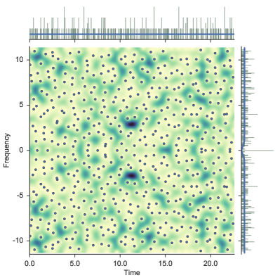
(a) Real white noise/symmetric GAF

(b) Complex white noise/planar GAF

Figure 1: The spectrogram of (a) a realization of real white noise, and (b) a realization of complex white noise. The right and top plots on each panel show marginal histograms, superimposed with the theoretical marginal density, see text for details.

Coming back to our problem of detecting signals, this non-stationarity makes it uneasy to approach via traditional spatial statistics techniques, which often assume some degree of stationarity. However, there is a stationary point process that is a good approximation for the zeros of the symmetric planar GAF, and that has been studied in depth. This point process is the zeros of the planar GAF, the entire function corresponding to the STFT of complex white noise.

4 The case of complex white noise

We now introduce the planar GAF, and explain why its zeros are a good approximation to those of the symmetric planar GAF. In other words, we justify why the spectrogram of the real white Gaussian noise can be approximated by that of the complex white Gaussian noise. We conclude by considering the analytic white noise.

4.1 Definitions

Consider the two-dimensional white noise of (Holden et al., 2010, Section 2.1.2), that is, the space $\mathcal{S}^{\prime}\times\mathcal{S}^{\prime}$, with the Borel $\sigma$-algebra associated to the product weak star topology, and measure $\mu_{1}\times\mu_{1}$. A draw ${\boldsymbol{\xi}}=(\xi_{1},\xi_{2})\sim\mu_{1}\times\mu_{1}$ consists of two independent white noises. Letting $\boldsymbol{\phi}=(\phi_{1},\phi_{2})$ in $\mathcal{S}\times\mathcal{S}$, we define the smoothed complex white noise as in (Holden et al., 2010, Exercise 2.26) through

$$w(\boldsymbol{\phi},\xi)=\langle\xi_{1},\phi_{1}\rangle+i\langle\xi_{2},\phi_{2}\rangle,$$

where ${\boldsymbol{\xi}}\sim\mu_{1}\times\mu_{1}$. It is called “smoothed” because we define it using a pair of test functions $\boldsymbol{\phi}$, which will be enough for our purpose. Note also that in signal processing, this is typically called a proper or circular Gaussian white noise (Picinbono and Bondon, 1997).

Now, if we let both test functions be $t\mapsto M_{v}T_{u}g$, we recover what can reasonably be called the STFT of complex white noise

$$u,v\mapsto\langle\xi_{1},M_{v}T_{u}g\rangle+i\langle\xi_{2},M_{v}T_{u}g\rangle.$$ (13)

4.2 Characterizing the zeros

The same arguments as in the proofs of Propositions 2 and 3 lead to

Proposition 4.

With $\mu_{1}\times\mu_{1}$ probability $1$, the zeros of the STFT (13) are those of the entire function

$$\frac{1}{\sqrt{2}}\sum_{k=0}^{\infty}\left(\langle\xi_{1},h_{k}\rangle+i\langle\xi_{2},h_{k}\rangle\right)\frac{\pi^{k/2}z^{k}}{\sqrt{k!}},$$ (14)

where $z=u+iv$.

We note that under $\mu_{1}\times\mu_{1}$, the random variables $2^{-1/2}(\langle\xi_{1},h_{k}\rangle+i\langle\xi_{2},h_{k}\rangle)$ are i.i.d. unit complex Gaussians, and the entire function (14) is called the planar Gaussian analytic function in the literature. In particular, the planar GAF is one of the three fundamental GAFs in the monograph of Hough et al. (2009), and more is known about its zeros than for the symmetric planar GAF in Proposition 3. We group some known results in Proposition 5, selecting results that could be of statistical use in signal processing.

Proposition 5 (Hough et al. (2009); Nishry (2010)).

The planar GAF satisfies the following properties:

1. The distribution of its zeros is invariant to rotations and translations in the complex plane (Hough et al., 2009, Proposition 2.3.7). In particular, it is a stationary point process.

2. Its correlation functions are known (Hough et al., 2009, Corollary 3.4.2). In particular, the intensity in constant equal to $1$, and with the notation of Section 2.4, for $z,z^{\prime}\in\mathbb{C}$ such that $|z-z^{\prime}|=r$, the pair correlation function reads

   $$\rho^{(2)}(z,z^{\prime})=g_{0}(r)=\frac{\left[\sinh^{2}\left(\frac{\pi r^{2}}{2}\right)+\frac{\pi^{2}r^{4}}{4}\right]\cosh\left(\frac{\pi r^{2}}{2}\right)-\pi r^{2}\sinh(\frac{\pi r^{2}}{2})}{\sinh^{3}\left(\frac{\pi r^{2}}{2}\right)}.$$ (15)

3. The hole probability

   $$p_{r}=\mathbb{P}(\text{no points in the disk centered at $0$ and with radius $r$})$$

   scales as

   $$r^{-4}\log p_{r}\rightarrow-3e^{2}/4$$ (16)

   as $r\rightarrow+\infty$ (Nishry, 2010).

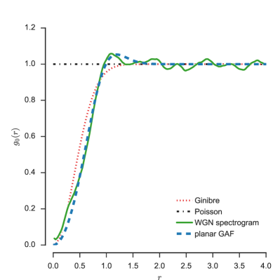
(a) Pair correlation functions $g_{0}$

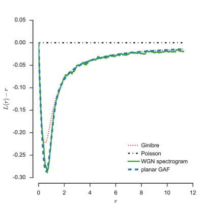
(b) $r\mapsto L(r)-r$ functional statistics

Figure 2: Comparison of the Ginibre point process, the zeros of the planar GAF, and a realization of the zeros of the spectrogram of complex white noise, using (a) pair correlation functions $g_{0}$, and (b) the $L$ functional statistic, see Section 2.4 for definitions.

Figure 2 illustrates Proposition 5. We plot the pair correlation function (15) of the planar GAF, along with the pair correlation functions of the Poisson and Ginibre point processes introduced in Section 2.4. We also superimpose an estimate of $g_{0}$ obtained from the spectrogram of a realization of a complex white noise, see Section 5 for computational procedures. Finally, we also plot the $L$ functional statistic for the same point processes, as introduced in Section 2.4.

Both the planar GAF and Ginibre are repulsive at small scales, but the planar GAF alone has a small ring of attractivity around $r=1$, well visible in Figure 2(a). This implies that the zeros of the planar GAF cannot be a DPP with Hermitian kernel, as introduced in Section 2.4.2, unlike what we and Flandrin (2017) may have intuited. DPPs were indeed a good candidate for the zeros, as they are repulsive point processes and naturally relate to reproducing kernel Hilbert spaces, such as those behind the STFT (Gröchenig, 2001, Theorem 3.4.2). But the zeros of the planar GAF show no repulsion at large scales, and more importantly the pair correlation function (15) is larger than $1$ around $r=1$, while the pair correlation of a DPP with Hermitian kernel cannot exceed 1 by definition (6). Note that strictly speaking, it is still possible that the zeros of the planar GAF are a DPP with a non-Hermitian kernel.

Even if they are not a DPP with Hermitian kernel, the zeros of the planar GAF are often compared to the Ginibre ensemble, which is a DPP and is also invariant to isometries of the plane (Hough et al., 2009, Section 4.3.7). In particular, the decay of the log hole probability (16) is also in $r^{4}$ for the Ginibre process (Hough et al., 2009, Proposition 7.2.1). This is to be compared to the slower decay in $r^{2}$ of a Poisson process with constant rate. This is an indication that locally, the zeros of the planar GAF and the Ginibre ensemble are similarly rigid or regularly spread, and that both are more rigid than Poisson. There are other intriguing similarities between the two point processes, see (Krishnapur and Virág, 2014), where Ginibre is shown to be the zeros of a GAF with a randomized kernel.

4.3 The zeros of the planar GAF approximate those of the symmetric planar GAF

To sum up, the spectrogram of real white noise is described by the symmetric planar GAF, but the zeros of the planar GAF are more amenable to further statistical processing. In this section, we survey results by Feldheim (2013) and Prosen (1996) that support approximating the zeros of the symmetric planar GAF by those of the planar GAF.

The zeros of the symmetric planar GAF (12) have the same distribution as the zeros of

$$f_{\text{sym}}(z)=e^{-\frac{\pi}{2}z^{2}}\sum_{k=0}^{\infty}\frac{a_{k}}{\sqrt{k!}}\pi^{k/2}z^{k},$$ (17)

where $a_{k}$ are i.i.d. unit real Gaussians. Note that the covariance kernel of $f_{\text{sym}}$ is

$$K_{\text{sym}}(z,w) \triangleq \mathbb{E}f_{\text{sym}}(z)\overline{f_{\text{sym}}(w)}$$

$$= e^{-\frac{\pi}{2}z^{2}}e^{-\frac{\pi}{2}\bar{w}^{2}}e^{\pi z\bar{w}}$$

$$= e^{-\frac{\pi}{2}(z-\bar{w})^{2}}.$$

This hints some invariance of $f_{\text{sym}}$ to translations along the real axis. By a limiting argument, see e.g. (Hough et al., 2009, Lemma 2.3.3), (17) is indeed a stationary symmetric GAF in the sense of Feldheim (2013). Namely, for any $n$, any $z_{1},\dots,z_{n}$, and any $t\in\mathbb{R}$, $\left(f_{\text{sym}}(z_{1}+t),\dots,f_{\text{sym}}(z_{n}+t)\right)$ has the same distribution as $\left(f_{\text{sym}}(z_{1}),\dots,f_{\text{sym}}(z_{n})\right)$.

Feldheim (2013) derives the intensity of the zeros of general stationary symmetric GAFs. More precisely, let $n_{\text{sym}}(B)$ be the random number of zeros of $f_{\text{sym}}$ in a Borel set $B\subset\mathbb{C}$, she says that there exists a so-called horizontal counting measure $\nu_{\text{sym}}$ s.t., almost surely, we have the weak convergence of measures

$$\nu_{\text{sym}}(A)=\lim_{T\rightarrow\infty}\frac{n_{\text{sym}}([0,T]\times A)}{T},$$

where $A$ is a Borel set on the vertical axis. In other words, $\nu_{\text{sym}}$ characterizes the density of zeros averaged across the horizontal axis. For our symmetric planar GAF (17), (Feldheim, 2013, Theorem 1) yields

$$\nu_{\text{sym}}(A) = \int_{A}\left[dS(y)+\delta_{0}\right],$$ (18)

where

$$S(y)=\frac{y}{\sqrt{1-e^{-4\pi y^{2}}}}.$$

Equation (18) is the sum of a continuous component and a Dirac mass at $0$. The Dirac mass relates to the accumulation of zeros on the real axis discussed in Section 3. The numerator of the continuous part $S$ is the unnormalized cumulative density of a uniform distribution, and the denominator quickly converges to $1$ as $y$ grows.

Now compare (18) to the horizontal counting measure of the zeros of the planar GAF, which is simply the uniform $dy$, without any atom, see e.g. (Feldheim, 2013, Theorem 1) again. We observe that the two counting measures are quickly approximately equal, as one goes away from the real axis. More precisely, for $A\subset[1,+\infty)$, the ratio of $S(A)$ by the Lebesgue measure of $A$ is within $2\cdot 10^{-6}$ of $1$. For Gaussian windows of arbitrary width, the change of variables (3) yields that the approximation is tight for $\text{Im}(z)\geq a$. This is no obstacle in signal processing practice, as spectrograms are never considered close to the real axis, where ’close’ is defined by the spread of the observation window in frequency, which is of order $a$, see Section 4.4. We also plot the densities of the continuous part of both measures in Figure 1. The Dirac mass of the symmetric planar GAF corresponds to the subset of zeros on the real axis.

A natural question is whether the approximation is also accurate for higher-order interactions in the two point processes. This question can be addressed by comparing $k$-point correlation functions. The case of the planar GAF was derived by Hannay (1998), and closed-form formulas are derived for the symmetric planar GAF in (Prosen, 1996, Equation (12)). The latter are not easy to interpret as they involve nonstandard combinatorial combinations of matrix coefficients. Still, (Prosen, 1996, Equation 25) shows that when $\text{Im}(z)\gg 0$, the $k$-point correlation functions of the zeros of the symmetric planar GAF are well approximated by those of the zeros of the planar GAF.

To conclude, the distribution of the zeros of the STFT of real white Gaussian noise is well approximated by that of complex white Gaussian noise, as long as the observation window is sufficiently far from the time axis.

4.4 On the analytic white noise

A real-valued function $f\in L^{2}$ has an Hermitian Fourier transform. In signal processing, it is thus common to cancel out the negative frequencies of a real-valued signal $f\in L^{2}$ by defining a complex-valued associated function called its analytic signal,

$$f^{+}(x)=2\mathcal{F}^{-1}(\mathbbm{1}_{\mathbb{R}_{+}}\mathcal{F}f)(x),\forall x\in\mathbb{R}.$$ (19)

where $\mathcal{F}$ is the usual Fourier transform. The term “analytic” is related to the alternative definition of $f^{+}$ as the boundary function of a particular holomorphic function on the lower half of the complex plane, see e.g. (Pugh, 1982, Section 2.1) for a concise and rigorous treatment. In signal processing practice, beyond removing redundant frequencies, the modulus and argument of $f^{+}$ have meaningful interpretations for elementary signals (Picinbono, 1997). Since our initial goal is to understand the behaviour of the zeros of a real white noise, it is thus tempting to define and consider an analytic white noise to represent this real white noise. If this approach led to a simple statistical characterization of zeros, then we would avoid the approximation by the complex white noise of Section 4.1.

While folklore has it that the analytic white noise is the circular white noise of Section 4.1, this is not the case for the most natural definition of the analytic signal of a distribution. Following (Pugh, 1982, Section 3.3), we define in this paper the analytic white noise by its action on $L^{2}$: letting $\xi\sim\mu_{1}$ be a real white noise, we take

$$\langle\xi^{+},f\rangle\triangleq 2\langle\xi,\mathcal{F}^{-1}(\mathbbm{1}_{\mathbb{R}_{+}}\mathcal{F}f)\rangle,\qquad\forall f\in L^{2}.$$ (20)

For our purpose, it is enough to consider $\xi^{+}$ through its action (20). In particular, if we want to follow the lines of Sections 3 and 4 and identify the general term of a random series corresponding to the STFT of $\xi^{+}$, we need an orthonormal basis $(\zeta_{k})$ of $L^{2}$ and a window $g$ such that

$$\langle\zeta_{k},\mathcal{F}^{-1}(\mathbbm{1}_{\mathbb{R}_{+}}\mathcal{F}M_{v}T_{u}g)\rangle$$ (21)

is known in closed-form and simple enough. Hermite functions and the Gaussian window definitely do not satisfy our criteria anymore, and we leave this existence as an open question. Still, we have the following heuristic argument: when $g$ is the unit-norm Gaussian, (21) becomes

$$\langle\zeta_{k},\mathcal{F}^{-1}(\mathbbm{1}_{\mathbb{R}_{+}}T_{v}M_{-u}g)\rangle,$$ (22)

so that when $v$ is large enough, say a few times the width of the window $g$, $T_{v}M_{-u}g$ puts almost all its mass on $\mathbb{R}_{+}$, and the indicator in (22) can be dropped. The Hermite basis then satisfies our requirements, giving the planar GAF of Section 4. Intuitively, far from the real axis, the spectrogram of the analytic white noise will look like that of proper complex white noise. This heuristic is to relate to standard time-frequency practice, where one leaves out of the spectrogram a band that is within the width of the window of the lower half plane. This is meant to avoid taking into account both positive and negative frequencies of the signal simultaneously.

5 Practical spatial statistics using the zeros of the STFT

In Section 5.1, we discuss how to relate the continuous complex plane $\mathbb{C}$ with the practical discrete implementation of the Fourier transform. In Section 5.2, we investigate simple hypothesis tests for signal detection, as in (Flandrin, 2015).

5.1 Going discrete

To fully bridge the gap with numerical signal processing practice, there is an additional level of approximation that needs to be discussed: Continuous integrals are replaced by discrete Fourier transforms, so that the fast Fourier transform can be used. We first describe an experimental setting to study the zeros of the spectrogram of Gaussian white noise. In particular, we explain how to reach an asymptotic regime where the noise occupies an infinite range both in time and frequency and the spectrogram is infinitely well resolved. Second, we investigate practical issues related to detecting a signal in white noise by using its influence on the distribution of zeros of the spectrogram.

5.1.1 Zeros of noise only

Let $F_{s}$ the sampling frequency, $\Delta t=1/F_{s}$ the time sampling step size and $T$ the duration of the observation window. The number of samples is then $N+1$ with $N=T/\Delta t$.

Let $K$ be the length of the discretized Gaussian analysis window, i.e. its duration is $K\Delta t$; therefore $\Delta\nu=F_{s}/K=1/K\Delta t$ is the frequency sampling step. In practice, the spectrogram obtained from a discrete STFT is then an array of size $(N+1,K/2+1)$. Then we consider the time-frequency domain $[0,T]\times[0,F_{s}/2]$ only; it corresponds to the analytic signal. This is due to the Hermitian symmetry of the Fourier transform of real signals: negative frequencies do not add any information to that carried by positive frequencies, see also Section 4.4. This Hermitian symmetry can also be seen on the zeros of the symmetric GAF in Figure 1(a), where signal processing practice would have us only consider the upper half-plane ($\nu\geq 0$). From Feldheim (2013)’s results, see (18), we know that the expected number of zeros of the continuous spectrogram is close to $TF_{s}/2$ if we neglect the (asymptotically negligible) region $|\nu|\leq a$ close to the time axis, see Section 4.3. Assuming that we are able to extract every zero, the expected number of zeros in the discrete spectrogram is then $TF_{s}/2=N/2$ in very good approximation.

Let $\sigma_{t}=1/(a\sqrt{2\pi})$ and $\sigma_{\nu}=1/(2\pi\sigma_{t})$ denote the spreads of the Gaussian analysis window $g_{a}$ in time and frequency, respectively. Note that the scale $a$ serves as a fixed reference for scales in the sequel. We would like to retain the stationary properties of the planar GAF in our discrete STFTs. We thus require that, in the discrete setting, the resolution – in number of points – should be the same in time and frequency, that is

$$\frac{\sigma_{t}}{\Delta t}=\frac{\sigma_{\nu}}{\Delta\nu}\Longleftrightarrow\sigma_{t}\cdot F_{s}=\sigma_{\nu}\cdot K\Delta t$$ (23)

This leads to

$$\left(\frac{\sigma_{t}}{\Delta t}\right)^{2}=\frac{K}{2\pi}\Leftrightarrow\sigma_{t}=\sqrt{\frac{K}{2\pi}}\Delta t.$$ (24)

If we want to study the spectrogram of continuous white noise over an infinite time-frequency domain, numerical simulations must obey two necessary conditions:

$$\begin{cases}\text{infinite duration }\Leftrightarrow\text{fine frequency resolution}&:T/\sigma_{t}=2\pi\sigma_{\nu}/\Delta\nu\rightarrow+\infty\\ \text{infinite frequency range }\Leftrightarrow\text{fine time resolution}&:F_{s}/\sigma_{\nu}=2\pi\sigma_{t}/\Delta t\rightarrow+\infty\\ \end{cases}$$ (25)

In terms of samples, these two conditions imply that $N,K\rightarrow\infty$. More precisely,

$$\frac{\sigma_{t}}{T} = \frac{1}{N}\sqrt{\frac{K}{2\pi}}\rightarrow 0\text{ as }N,K\rightarrow\infty$$ (26)

$$\frac{\sigma_{\nu}}{F_{s}} = \frac{1}{\sqrt{2\pi K}}\to 0\text{ as }N,K\rightarrow\infty.$$ (27)

These conditions are directly satisfied for $K\propto N$, where $\propto$ means “proportional to”. Note that in practice because of border effects one chooses $N=2K$ and keeps the $N$ samples whose time index $n$ is such that $K/2\leq n\leq N-K/2$. Then, $\sigma_{\nu}/F_{s}=1/\sqrt{2\pi K}\propto 1/\sqrt{N}$, $\sigma_{t}/T\propto 1/\sqrt{N}$; note that $\Delta t/\sigma_{t}=\Delta\nu/\sigma_{\nu}\propto 1/\sqrt{N}$ as well. As a result, simulations can asymptotically well approximate the continuous spectrogram of Gaussian white noise.

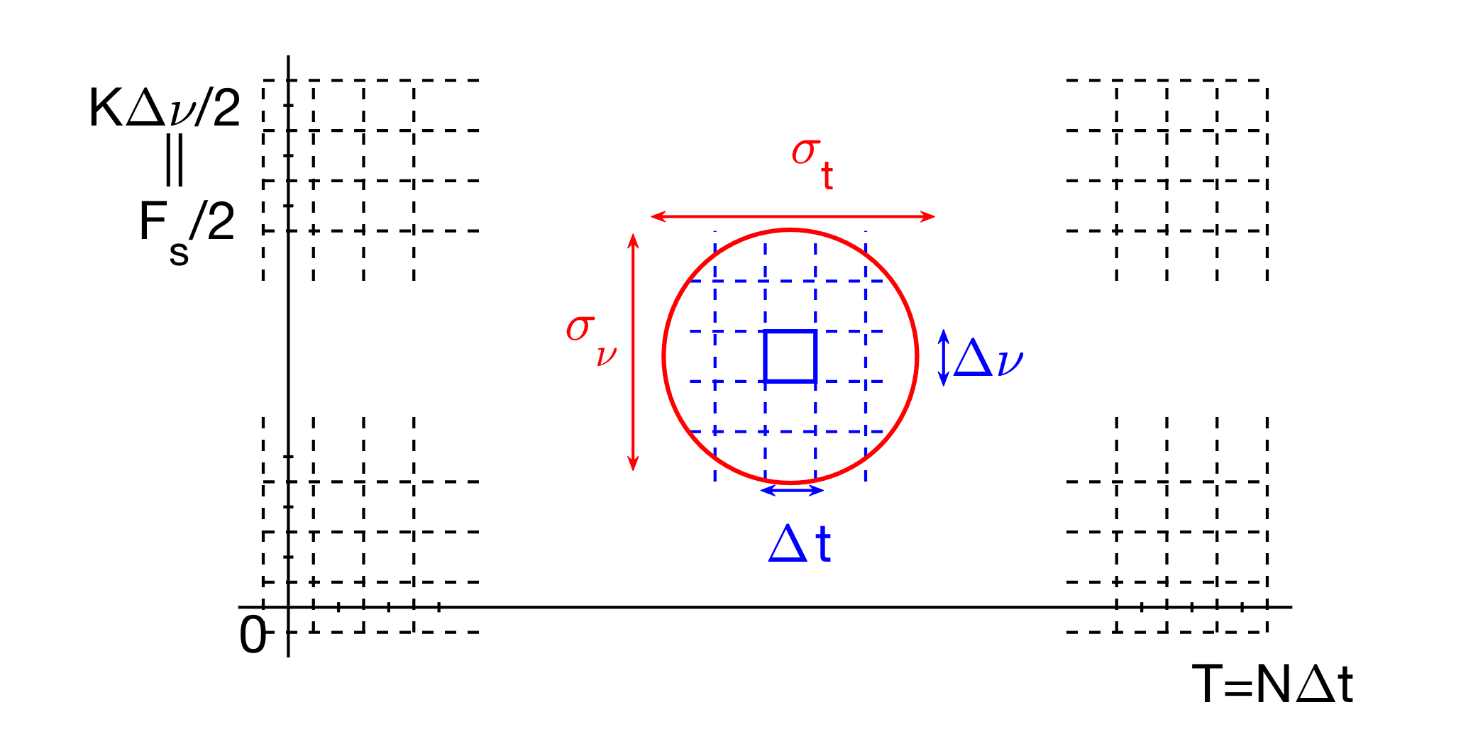
Figure 3: Illustration of the discrete time-frequency plane $\{(n\Delta t,k\Delta\nu),\;0\leq n\leq N-1,\;0\leq k\leq K/2\}$. The resolution of the spectrogram is controlled by the analysis window’s Gabor parameters $(\sigma_{t},\sigma_{\nu})$.

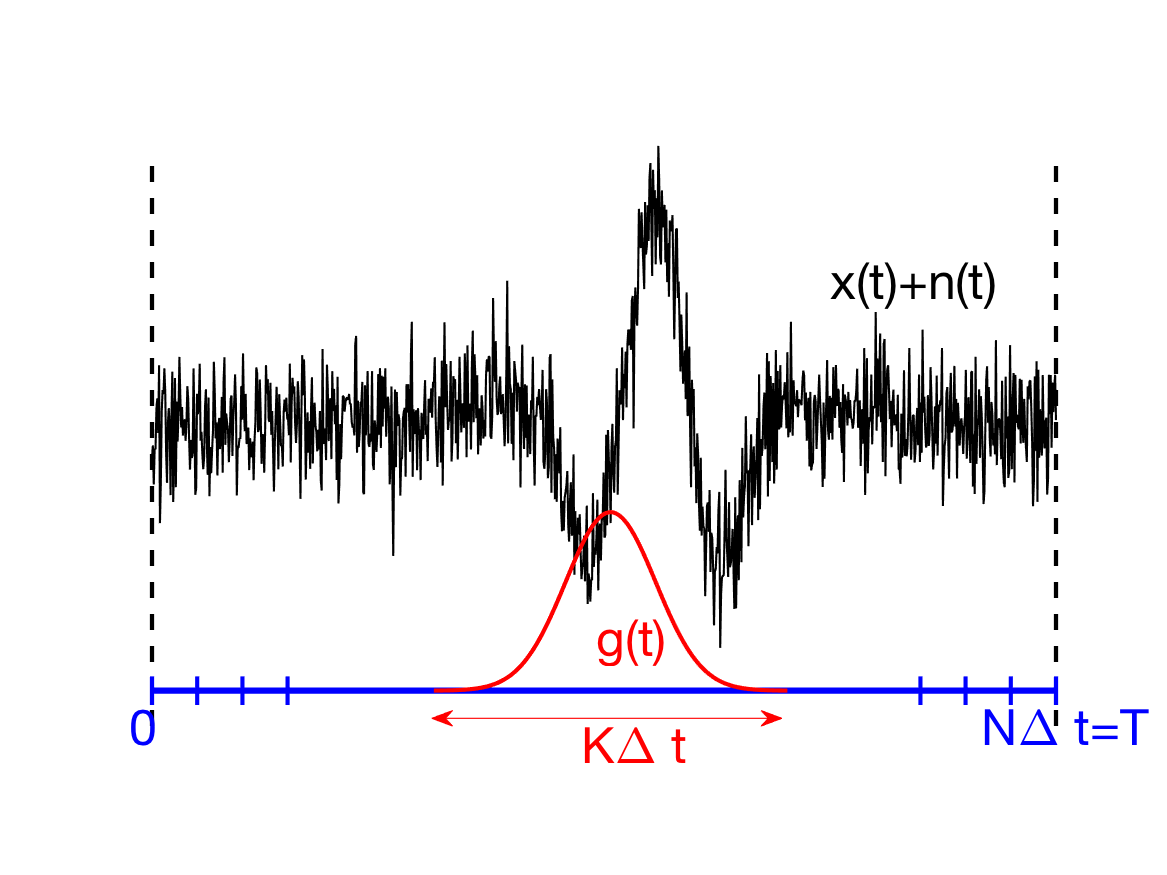
Figure 4: Illustration of the STFT: the noisy signal is convolved with a Gaussian that is translated in time and frequency. The colour code corresponds to Figure 3 for ease of reference.

Figure 3 illustrates the relative scales of the duration $T=N\Delta t$, the frequency range $K/2\Delta t$ (for $\nu\geq 0$), the time and frequency resolutions $\Delta t$ and $\Delta\nu$, as well as the resolution of the time-frequency kernel corresponding to the window $g(t)$ with Gabor spread $(\sigma_{t},\sigma_{\nu})$. For the sake of completeness and the reader new to time-frequency, we include in Figure 3 an illustration of the STFT of a noisy signal.

Now we detail how to relate the discrete coordinates of a discrete spectrogram with the continuous complex plane. For a given value of $a$, one has $\sigma_{t}=1/(a\sqrt{2\pi})$ and thus making the correspondence between samples and time-frequency units implies setting $\Delta t=\sqrt{2\pi/K}\sigma_{t}$. For $a=1$ one has $\Delta t=\sqrt{1/K}$ so that $u=n/\sqrt{K}$ and $v=k/\sqrt{K}$ are the coordinates of the time-frequency plane corresponding to time sample $n$ and frequency sample $k$, respectively. Figure 5 depicts the whole numerical simulation procedure. It represents the simulated spectrogram and the corresponding extracted area, taking border effects in consideration. The bound $\ell$ fixes how many samples close to the zero-frequency axis should be removed. For $a=1$, we have chosen $\ell=\sqrt{K}$, at it corresponds to $y=1$ in (18). Note also that border effects alone would actually allow us to extend the shaded square in Figure 5 on its left and right to include $K$ samples. Instead, we chose to reduce it to $K/2-\ell$ mostly for esthetical concerns: since the point process we observe is almost stationary when only noise is present, we favoured a square window rather than a rectangle.

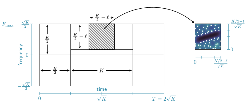
Figure 5: Numerical simulation procedure. Black ticks indicate the number of samples, while blue ticks show time-frequency units for a choice of $\Delta t=1/\sqrt{K}$ (see text for details). In other words, blue ticks are the coordinates in the complex plane that are implicit in the mathematical results of Sections 3 and 4. The dashed region corresponds to the area used in subsequent simulations.

When the conditions above are satisfied, several phenomena occur in the limit of infinite oversampling $N\to\infty$, which is equivalent to letting both the duration $T$ and the sampling frequency $F_{s}$ grow to infinity. In a dual manner, the resolution $(\Delta t,\Delta\nu)$ of the discrete spectrogram tends to zero. The time-frequency extent $(\sigma_{t},\sigma_{\nu})$ of the analysis window remains constant but is described by a number of samples that grows as $\sigma_{t}/\Delta t\propto\sqrt{N}$ while $\sigma_{t}/T\propto 1/\sqrt{N}\to 0$. The analysis window is thus more and more finely resolved, and we become close to a continuous description. In parallel, the expected number of zeros in the spectrogram of the white noise is $F_{s}T/2$ and tends to $\infty$ as $N$ grows. Therefore, assuming perfect zero detection, statistics such as Ripley’s $K$ function or the variance-stabilized $L$ functional statistic of Section 2.4.3 can be asymptotically perfectly well estimated.

In practice, we defined a numerical zero as a local minimum among its eight neighbouring bins, and found that the number of zeros was consistent with what we expected from Proposition 5, even if we did not impose a threshold on the value of the spectrogram at the local minimum.

We leave this section on a mathematical note. In this section, we implicitly assumed that in the limit on an infinite observation window and an infinite sampling rate, the discrete Fourier transforms involved in the computation of the discrete spectrogram converge to their continuous counterpart. For the sake of completeness, we mathematically justify in what sense this convergence can be expected. With the notation of Section 3, subdivide again $[0,T]$ into $N$ equal intervals and denote by $\chi_{n}$ the indicator of the $n$th interval $[(n-1)\Delta t,n\Delta t]$. Let $P_{N,T}:\mathcal{S}\rightarrow L^{2}$ attach to a Schwartz function $f$ the “sampled” simple function $\sum_{n=1}^{N}f(n)\chi_{n}$. Then $P_{N,T}f\rightarrow f$ in $L^{2}$ as $T$ and $N$ go to infinity and $T/\sqrt{N}\rightarrow\alpha>0$, which is the setting described above in this section. On the other hand,

$$\langle\xi,P_{N,T}M_{v}T_{u}g\rangle=\sum_{n=1}^{N}\langle\xi,\chi_{n}\rangle e^{-2i\pi vn\Delta t}g(n\Delta t-u)$$ (28)

is what we call the discrete STFT at $(u,v)$ of a realization of white noise. Note that in distribution, $(\langle\xi,\chi_{n}\rangle)_{n}$ is a sequence of i.i.d. Gaussians with variance $\Delta t$. To see how (28) is a good approximation to our initial continuous STFT, we note that for all $u,v$,

$$\mathbb{E}_{\mu_{1}}|\langle\xi,M_{v}T_{u}g\rangle-\langle\xi,P_{N,T}M_{v}T_{u}g\rangle|^{2} = \mathbb{E}_{\mu_{1}}|\langle\xi,M_{v}T_{u}g-P_{N,T}M_{v}T_{u}g\rangle|^{2}$$

$$= \|M_{v}T_{u}g-P_{N,T}M_{v}T_{u}g\|^{2}_{L_{2}}\rightarrow 0.$$

5.1.2 Zeros of signal plus noise

When a signal is present, its specific scales destroy the scale invariance property of Gaussian white noise and deprives us from any asymptotic regime in our numerical simulations. Let $A_{S}$ denote the typical time and frequency area occupied by the considered signal. The presence of this signal creates a region of the spectrogram of size $A_{S}$ where a decrease in the number of zeros is expected due to the positive amount of energy corresponding to the signal. This decrease is clearly visible in the spectrograms of Figure 7 for linear chirps with various $A_{S}$ and various signal-to-noise ratios (SNR). The approach proposed here to build statistical detection tests is based on this intuition. To this purpose one needs to quantify how far the presence of a signal can influence the statistics used in our tests so that we can maximize this influence and the efficiency of the proposed test.

Given a sampling rate $F_{s}$ and a duration of observation $T$, the unit intensity in Proposition 5 yields that the expected number of zeros in the spectrogram of a real white noise is $F_{s}\cdot T/2=N/2$, neglecting what happens at small frequencies close to the time axis. Note that this is independent of the width $(\sigma_{t},\sigma_{\nu})$ of the Gaussian analysis window $g$. If one wants to increase the number of zeros in the spectrogram to get better statistics, it is enough to increase either $F_{s}$ or $T$. However, the expected decrease in the number of zeros due to the presence of a signal is of the order of the area $A_{S}$, the finite time-frequency area $A_{S}$ corresponding to the spectrogram of the signal alone. As a consequence, an excessive increase in either $F_{s}$ and/or $T$ would result in an asymptotically complete dilution of the influence of the signal on the considered statistics. Thus, our purpose is to build statistics over one or more patches $P$ of the spectrogram of maximal area $A_{P}=\eta_{t}\eta_{\nu}$ such that $A_{S}/A_{P}\simeq 1$. On one hand, a maximal area $A_{P}$ is necessary to ensure that the estimate of the chosen statistic be as accurate as possible (in particular in the presence of noise only, to take into account as many zeros as possible and minimize the false positive detection rate); on the other hand, this statistic will be more sensitive to the presence of a signal if it mostly depends on the influence of the signal on the distribution of zeros in the spectrogram (in particular, in the presence of signal, we maximize the true positive detection rate). In practice, note that one can hope to detect only signals such that $A_{S}\gg\sigma_{t}\sigma_{\nu}=1/2\pi$, which means signals with a time-frequency support that affects more than $\sigma_{t}/\Delta t\cdot\sigma_{\nu}/\Delta\nu=K/2\pi$ samples of the spectrogram.

5.2 Detecting signals through hypothesis testing

5.2.1 Monte Carlo envelope tests

In Section 2.4.3, we reviewed some popular functional statistics for stationary isotropic point processes. We focus here on $L$, the variance-stabilized version of Ripley’s $K$ function, and the empty space function $F$, see Section 2.4. We follow classical Monte Carlo testing methodology based on functional statistics, which we now sketch, see e.g. (Baddeley et al., 2014) for a less concise introduction.

The methodology is independent of the test statistic used, so we introduce it for a general functional statistic $r\mapsto S(r)$, which we later instantiate to be $L$ or $F$. Let $\hat{S}$ denote an empirical estimate obtained from the spectrogram of data, possibly using edge corrections, see (Møller and Waagepetersen, 2003). Let $S_{0}$ be the theoretical functional statistic corresponding to complex white noise. For $S=L$, $L_{0}$ can be easily computed from (15). Note that our noise is real white noise in the applications, but we approximate the corresponding 2-point correlation function by that of complex white noise far from the real axis, as explained in Section 4.3. Detection of signal over white noise can be formulated as testing the hypothesis $H_{0}$ that $\hat{S}$ was built from a realization of a real white noise, versus the alternate hypothesis $H_{1}$ that it was not. To do this, we review Monte Carlo envelope-based hypothesis tests, which are popular across applications.

In a Monte Carlo envelope test, we define a test statistic $T\in\mathbb{R}$ that summarizes the difference $r\mapsto S(r)-S_{0}(r)$ in a single real number, for instance a norm

$$T_{\infty}=\sup_{r\in[r_{\min},r_{\max}]}|S(r)-S_{0}(r)|\qquad\text{ or }\qquad T_{2}=\sqrt{\int_{r_{\min}}^{r_{\max}}|S-S_{0}|^{2}}.$$ (29)

Let $t_{\text{exp}}$ denote the realization of $T$ corresponding to the experimental data to be analyzed. The test consists in simulating $m$ realizations of white noise, obtaining the corresponding functional statistics estimates $S_{1},\dots,S_{m}$, computing the realizations $t_{1},\dots,t_{m}$ of the test statistic, and rejecting $H_{0}$ whenever the observed $t_{\text{exp}}$ is larger than the $k$-th largest value among $t_{1},\dots,t_{m}$. Without loss of generality, we assume $t_{1},\dots,t_{m}$ are in decreasing order, so that $t_{k}$ is the $k$-th largest. Symmetry considerations show that this test has significance level $\alpha=k/(m+1)$. When $S_{0}$ is not available in closed form, one can replace it by a pointwise average

$$\bar{S}_{0}(r)=\frac{1}{m+1}(S_{1}(r)+\dots+S_{m}(r)+\hat{S}(r))$$ (30)

while preserving the significance level, see (Baddeley et al., 2014).

To see why this test is called an envelope test, let $k=10$ and $m=199$ so that $\alpha=0.05$. We use as a signal a synthetic chirp plus white noise as in Figure 7, with SNR$=20$. In Figure 6, we take $r_{\min}=0$ and let $r_{\max}$ vary, showing for each $r_{\max}$ the corresponding $t_{k}$ as the upper limit of the green shaded envelope. The black line shows $t_{\text{exp}}$ at each $r_{\max}$, for the same realizations of the tested signal and the white noise spectrograms. To interpret this plot, imagine the user had fixed $r_{\max}$ to some value, then he would have rejected $H_{0}$ if and only if the corresponding intersection of the black line with $r=r_{\max}$ was above the green area. Note that the significance of the test in only guaranteed if $r_{\max}$ is fixed prior to observing data or simulations. Still, Figure 6 gives a heuristic to identify characteristic scales of interaction after $H_{0}$ is rejected. For instance, characteristic scales could be values of $r_{\max}$ where the data curve in black leaves the green envelope. The user can thus identify regions of the spectrogram that possibly correspond to signal (defined as ”different from white noise”). To illustrate this, consider again both plots of Figure 6. There is a hint of an interaction – an excess or deficit of pairs– between $r_{\max}=0.5$ and $r_{\max}=1$, and this interaction cannot be explained by noise only. Although we do not delve further here and rather focus on how the power of the test varies with parameters, this scale can be used to filter out the noise, in the manner of the Delaunay-based filtering of Flandrin (2015).

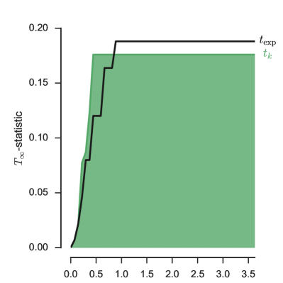
(a) $T_{\infty}$

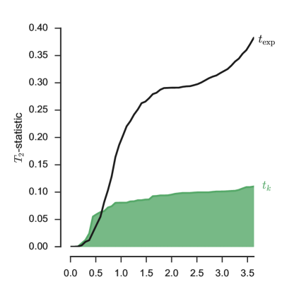
(b) $T_{2}$

Figure 6: Envelope plots for the detection test of Section 5.2 for the supremum and 2-norm of the deviation of the $L$ functional statistic from its pointwise average (30).

5.2.2 Assessing the power of the test

The significance $\alpha$ of the test – the probability of rejecting $H_{0}$ while $H_{0}$ is true – is fixed by the user as in Section 5.2.1. It remains to investigate the power $\beta$ of the test, that is, the probability of rejecting $H_{0}$ when one should. Following Section 5.1.2, we expect $\beta$ to increase with SNR, which should be large enough to “push” zeros away from the time-frequency support of the signal to be detected. We also expect the power to be larger when the observation window is not too much larger than the time-frequency support $A_{S}$ of the signal.

We back these claims by the experiment in Figure 7, where we assume signals take the form of linear chirps. Still taking $m=199$ and $k=10$, so that $\alpha=0.05$, we build each of the six panels as follows: we simulate a mock signal made using a linear chirp plus noise, with SNR indicated on the plot, growing from left to right. We then repeat $200$ times: 1) simulate $m$ white noise spectrograms, 2) check wether $H_{0}$ is rejected for each value of $r_{\max}$. We can thus estimate the probability $\beta$ of rejecting $H_{0}$ for various choices of $r_{\max}$ the user could have made. We plot both the power using $S=L$ or $S=F$, choosing the $2-$norm in (29) and the empirical average (30). We estimate the functional statistics using the spatstat R package. To identify the statistical significance of our estimated powers, we plot Clopper-Pearson confidence intervals for $5$ values of $r_{\max}$, using a Bonferroni correction for the $10$ multiple tests involved on each plot, see e.g. Wasserman (2013). Finally, the top row of Figure 7 corresponds to a signal support that matches the size of the observation window, while the bottom row is half that. On each panel, an inlaid plot depicts the spectrogram for one realization of the signal corrupted by white noise. Spectrogram zeros are in white.

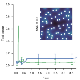
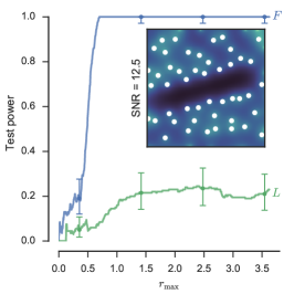
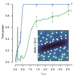
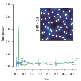
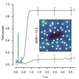
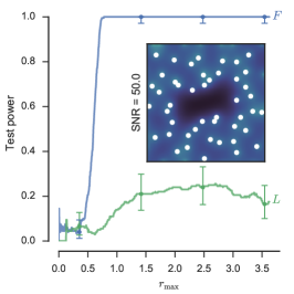
Figure 7: Assessing the power of the test on detecting a linear chirp with various SNRs across columns. The top row corresponds to a larger support of the chirp compared to the observation window.

The results confirm our intuitions: power increases with SNR, and decreases as the size of the support of the signal diminishes with respect to the observation window. In all experiments, the best power is obtained by taking $r_{\max}$ to be as large as possible, which here means half of the observation window. This makes sure that as many points/pairs as possible enter the estimation of the functional statistic $S$. Concerning the choice of functional statistic, the empty space function $F$ performs significantly better for high SNR and large enough $r_{\max}$. The green peaks of power at low $r_{\max}$ for some combinations of SNR and support are due to the excess of small pairwise distances introduced by the chirp signal. The power vanishes quickly once larger pairwise distances are considered, due to the cumulative nature of $L$. It is hard to rely on these peaks as they do not appear systematically and would require a careful hand-tuning of $r_{\max}$ that would likely defeat our purpose of automatizing detection. So overall, we would recommend using $F$ and large $r_{\max}$, which appears to be a robust best choice. We also found (not shown) first that $F$ is superior or equal to the other functional statistics described in Section 2.4 for chirp detection. Second, we found that the tests using the average (30) are consistently more powerful than those using the analytic form $L_{0}$ of $L$. We believe this is due to the edge correction that is implicitly made in (30), while the analytic $L_{0}$ corresponds to an infinite observation window. Third, we also observed the $2-$norm in (29) to be consistently more powerful than the supremum norm.

6 Discussion

We showed how to give a mathematical meaning to the zeros of the spectrogram of white noise, and investigated their statistical distribution for real, complex, and – to a lesser extent – analytical white noise. We have related these zeros to the zeros of Gaussian analytic functions, a topic of booming interest in probability. More pragmatically, we investigated the computational issues raised by implementing tests based on spectrogram zeros.

The connection with GAFs puts signal processing algorithms based on spectrogram zeros on firm ground, and further progress on GAFs is bound to be fruitful for signal processing. Perhaps less obviously, we believe signal processing tools can also bring insight into probabilistic questions on GAFs. For starters, the Bargmann transform, spectrogram zeros and the fast Fourier transform give a novel way to approximately simulate the zeros of the planar GAF, or even the zeros of random polynomials.

As for the detection of signals using spectrogram zeros, we have investigated the application of standard frequentist testing tools. They showed good power for high SNR, but the performance decreases for low SNR and small signal support compared to the observation window. There are various leads to improve on these two points. First, we could transform our global test into several local tests, trying to adapt the tested patch to the support of the signal. Second, models for signals could be fed to Bayesian techniques, allowing to explore all signals compatible with a given pattern of zeros.

Acknowledgments

We thank Patrick Flandrin, Adrien Hardy, and Fred Lavancier for fruitful discussions on various aspects of this paper. RB acknowledges support from ANR BoB (ANR-16-CE23-0003), and all authors acknowledge support from ANR BNPSI (ANR-13-BS03-0006).

References

- Baddeley et al. (2014) A. Baddeley, P. J. Diggle, A. Hardegen, T. Lawrence, R. K. Milne, and G. Nair. On tests of spatial pattern based on simulation envelopes. Ecological Monographs, 84(3):477–489, 2014.
- Cohen (1995) L. Cohen. Time-frequency analysis, volume 778. Prentice Hall PTR Englewood Cliffs, NJ:, 1995.
- Daley and Vere-Jones (2003) D. J. Daley and D. Vere-Jones. An Introduction to the Theory of Point Processes. Springer, 2nd edition, 2003.
- Feldheim (2013) N. D. Feldheim. Zeroes of Gaussian analytic functions with translation-invariant distribution. Israel Journal of Mathematics, 195(1):317–345, 2013.
- Flandrin (1998) P. Flandrin. Time-frequency/time-scale analysis, volume 10. Academic press, 1998.
- Flandrin (2015) P. Flandrin. Time–frequency filtering based on spectrogram zeros. IEEE Signal Processing Letters, 22(11):2137–2141, 2015.
- Flandrin (2017) P. Flandrin. On spectrogram local maxima. In International Conference on Acoustics, Speech and Signal Processing (ICASSP), pages 3979–3983. IEEE, 2017.
- Gautschi (2004) W. Gautschi. Orthogonal polynomials: computation and approximation. Oxford University Press, USA, 2004.
- Gröchenig (2001) K. Gröchenig. Foundations of time-frequency analysis. Birkhäuser, 2001.
- Hannay (1998) J. H. Hannay. The chaotic analytic function. Journal of Physics A: Mathematical and General, 31(49):L755, 1998.
- Holden et al. (2010) H. Holden, B. Øksendal, J. Ubøe, and T. Zhang. Stochastic partial differential equations. Springer, second edition, 2010.
- Hough et al. (2006) J. B. Hough, M. Krishnapur, Y. Peres, and B. Virág. Determinantal processes and independence. Probability surveys, 2006.
- Hough et al. (2009) J. B. Hough, M. Krishnapur, Y. Peres, and B. Virág. Zeros of Gaussian analytic functions and determinantal point processes, volume 51. American Mathematical Society Providence, RI, 2009.
- Krishnapur and Virág (2014) M. Krishnapur and B. Virág. The Ginibre ensemble and Gaussian analytic functions. International Mathematics Research Notices, 2014(6):1441–1464, 2014.
- Lavancier et al. (2014) F. Lavancier, J. Møller, and E. Rubak. Determinantal point process models and statistical inference. Journal of the Royal Statistical Society, 2014.
- Macchi (1975) O. Macchi. The coincidence approach to stochastic point processes. Advances in Applied Probability, 7:83–122, 1975.