A high-order wideband direct solver for electromagnetic scattering from bodies of revolution

Abstract

The generalized Debye source representation of time-harmonic electromagnetic fields yields well-conditioned second-kind integral equations for a variety of boundary value problems, including the problems of scattering from perfect electric conductors and dielectric bodies. Furthermore, these representations, and resulting integral equations, are fully stable in the static limit as $\omega\to 0$ in multiply connected geometries. In this paper, we present the first high-order accurate solver based on this representation for bodies of revolution. The resulting solver uses a Nyström discretization of a one-dimensional generating curve and high-order integral equation methods for applying and inverting surface differentials. The accuracy and speed of the solvers are demonstrated in several numerical examples.

Keywords: Maxwell’s equations, second-kind integral equations, magnetic field integral equation, generalized Debye sources, perfect electric conductor, penetrable media, body of revolution

1 Introduction

In isotropic homogenous media, the time-harmonic Maxwell’s equations (THME) governing the propagation of electric and magnetic fields are given by [41]

$$\nabla\times\bm{{\mathcal{E}}} =i\omega\mu\bm{\mathcal{H}}, \qquad\nabla\times\bm{\mathcal{H}} =\bm{\mathcal{J}}-i\epsilon\omega\bm{{\mathcal{E}}},$$ (1.1)

$$\nabla\cdot\bm{{\mathcal{E}}} =\frac{\rho}{\epsilon}, \nabla\cdot\bm{\mathcal{H}} =0,$$

where $\bm{{\mathcal{E}}}$ and $\bm{\mathcal{H}}$ are the electric and magnetic fields, respectively, and $\omega$ is the angular frequency. The electric charge is denoted by $\rho$ and the electric current by $\bm{\mathcal{J}}$. The electric permittivity and magnetic permeability are given by $\epsilon$ and $\mu$, respectively, and assumed to be piecewise constant in all that follows. It will be useful to define the wavenumber $k$ as $k=\omega\sqrt{\epsilon\mu}$, and we assume that $\Im(k)\geq 0$ as well. The implicit time dependence of $e^{-i\omega t}$ on $\bm{{\mathcal{E}}}$, $\bm{\mathcal{H}}$ has been suppressed.

Maxwell’s equations in the above form provide a surprisingly accurate approximation to physical phenomena, and therefore their accurate numerical solution is of the utmost importance in many fields, such as radio-frequency component modeling [30], meta-material simulation [22], and radar cross-section characterizations [52]. Several computational methods for the solution to (1.1) are used in practice, including finite difference, finite element, spectral methods, and integral equation methods [35, 31, 37, 50]. Finite difference and finite element methods are particularly useful when the material parameters vary in space, especially when that variation is anisotropic.

On the other hand, when applicable – namely in complex geometries with piecewise constant material parameters – integral equation methods have significant advantages. They reduce the dimensionality of the problem to the boundary alone, satisfy the necessary radiation conditions in exterior domains, do not suffer from grid-based dispersion errors (particularly problematic at high frequencies), and are compatible with a variety of fast algorithms, leading to asymptotically optimal schemes. Two standard problems in electromagnetics – scattering from perfect electric conductors and dielectric bodies – fit exactly these assumptions [28]. While high-order accurate methods in arbitrary geometries in three dimensions are still under active development, there are several important applications of Maxwell’s equations in scattering from bodies of revolution [7, 34, 20, 32, 26, 33, 48], where surface representation and quadrature are more straightforward. In this context, it is possible to build very high-order accurate, quasi-optimal solvers using separation of variables and the Fast Fourier Transform (FFT) which scale roughly as $\mathcal{O}(N^{3/2})$, where $N$ is the total number of unknowns needed to fully discretize the body’s surface.

Despite the applicability of integral equation-based solvers to bodies of revolution, however, wideband solvers have yet to be implemented that are robust in the genus-one case and in the low-frequency regime. There are two principal difficulties here: (1) constructing high-order accurate Nyström methods (including quadrature) for the so-called modal Green’s functions [11] is somewhat technical, and (2) existing integral equation methods suffered from ill-conditioning due to dense-mesh breakdown and topological breakdown [12, 13, 15] in the static limit. The algorithm of the present paper, based on the recent generalized Debye source formulations of Maxwell fields [13, 15], overcomes both of these obstacles.

The past few years have seen several methodological developments in electrostatic and acoustic scattering from bodies of revolution that should be noted [25, 51]. The vector-valued case is treated in [33], but with the method of fundamental solutions [4, 17] rather than an on-surface boundary integral discretization. In this work, we provide a thorough discussion of the calculations required in the vector case, as it is more involved than the scalar case. There is a substantial literature on scattering from bodies of revolution in the electrical engineering community which we do not seek to review here. We refer the reader to the papers and books mentioned above. We will point out relevant previous work when discussing particular topics: quadrature, kernel evaluation, and integral equation conditioning.

The paper is organized as follows: Section 2 introduces the generalized Debye source formulation of Maxwell fields on general surfaces and formulates the relevant boundary value problems for scattering from perfect conductors and dielectric (penetrable) bodies. Section 3 derives the necessary formalism required for separating vector-valued functions in cylindrical coordinates on surfaces of revolution. Section 4 describes a high-order Nyström-type solver for electromagnetic scattering. This includes a discussion of quadrature, kernel evaluation, and surface differential application. We provide several numerical examples demonstrating our algorithm in Section 5 and then discuss extensions and drawbacks of the scheme in Section 6.

2 Generalized Debye sources

Classically, most integral equations for electromagnetic scattering problems have been derived in the Lorenz gauge. More precisely, the electric and magnetic fields are represented using a scalar potential $\varphi$ and vector potential $\bm{\mathcal{A}}$ [41]:

$$\bm{{\mathcal{E}}} =i\omega\bm{\mathcal{A}}-\nabla\varphi$$ (2.1)

$$\bm{\mathcal{H}} =\nabla\times\bm{\mathcal{A}},$$

with

$$\bm{\mathcal{A}}(\vectorsym{x})=\frac{1}{\mu}\int\frac{e^{ik|\vectorsym{x}-\vectorsym{x}^{\prime}|}}{4\pi|\vectorsym{x}-\vectorsym{x}^{\prime}|}\,\bm{\mathcal{J}}(\vectorsym{x}^{\prime})\,d\vectorsym{x}^{\prime},\qquad\varphi(\vectorsym{x})=\frac{1}{\epsilon}\int\frac{e^{ik|\vectorsym{x}-\vectorsym{x}^{\prime}|}}{4\pi|\vectorsym{x}-\vectorsym{x}^{\prime}|}\,\frac{\nabla\cdot\bm{\mathcal{J}}(\vectorsym{x}^{\prime})}{i\omega}\,d\vectorsym{x}^{\prime},$$ (2.2)

so that $\nabla\cdot\bm{\mathcal{A}}=i\omega\epsilon\mu\varphi$. In the case of the perfect electric conductor, using these representations yields the Electric Field Integral Equation (EFIE) by enforcing the condition that the tangential electric field vanishes. The Magnetic Field Integral Equation (MFIE) is derived from the fact that the tangential magnetic field must equal the surface current $\bm{\mathcal{J}}$. By taking linear combinations of these equations, one can derive various Combined Field Integral Equations (CFIE) [9] to avoid spurious resonances. However, unless additional preconditioners are used [10], the EFIE and CFIE suffer from what is known as dense-mesh low-frequency breakdown due to the division by $\omega$ in the scalar potential term, leading to catastrophic cancellation. This can be circumvented by introducing electric charge as an additional variable, subject to the consistency condition $\nabla\cdot\bm{\mathcal{J}}=i\omega\rho$, which is implied by Maxwell’s equations (1.1). In that case, we define the scalar potential as $\varphi=\mathcal{S}_{k}\rho/\epsilon$. Here, $\mathcal{S}_{k}$ denotes the single-layer potential operator, as in (2.2). Additional boundary conditions must be added because of the extra unknown, but this is straightforward. (See [44, 47, 46] for various charge-current formulations of scattering problems.) However, as noted in the introduction, the second form of low-frequency breakdown occurs in Maxwell’s equations, which we refer to as topological low-frequency breakdown [13]. This form of breakdown is characterized by increased ill-conditioning as $\omega\to 0$, with a singular limit in the static case. The generalized Debye source representation of Maxwellian fields overcomes both, by taking the genus into account and by using scalar variables rather than currents to avoid catastrophic cancellation [13, 15]. (An alternative robust formulation is the Decoupled Potential Integral Equation (DPIE) [47], which results in separate integral equations for $\bm{\mathcal{A}}$ and $\varphi$.)

For charge- and current-free regions with piecewise constant material parameters $\epsilon$, $\mu$, a simple re-scaling of the equations (1.1) is useful to reduce the dependency to only a single parameter $k$. To this end, we define

$$\vectorsym{E}^{\textnormal{tot}}=\sqrt{\epsilon}\bm{{\mathcal{E}}},\qquad\vectorsym{H}^{\textnormal{tot}}=\sqrt{\mu}\bm{\mathcal{H}},$$ (2.3)

The THME then take the form:

$$\nabla\times\vectorsym{E}^{\textnormal{tot}} =ik\vectorsym{H}^{\textnormal{tot}}, \qquad\nabla\times\vectorsym{H}^{\textnormal{tot}} =-ik\vectorsym{E}^{\textnormal{tot}},$$ (2.4)

$$\nabla\cdot\vectorsym{E}^{\textnormal{tot}} =0, \nabla\cdot\vectorsym{H}^{\textnormal{tot}} =0.$$

where, as before, $k=\omega\sqrt{\epsilon\mu}$. In electromagnetic scattering problems, the total fields $\vectorsym{E}^{\textnormal{tot}}$, $\vectorsym{H}^{\textnormal{tot}}$ consist of the superposition of a known, incoming field $\vectorsym{E}^{\textnormal{in}}$, $\vectorsym{H}^{\textnormal{in}}$ and an unknown scattered field $\vectorsym{E}$, $\vectorsym{H}$:

$$\vectorsym{E}^{\textnormal{tot}} =\vectorsym{E}+\vectorsym{E}^{\textnormal{in}}$$ (2.5)

$$\vectorsym{H}^{\textnormal{tot}} =\vectorsym{H}+\vectorsym{H}^{\textnormal{in}}.$$

Boundary conditions are enforced on the total fields, and the known incoming fields provide data for the resulting integral equations.

In the case of multiple-material (non-conducting) penetrable scattering, the values of $\epsilon$, $\mu$ in region $\ell$ will be denoted by $\epsilon_{\ell}$, $\mu_{\ell}$, and all relevant quantities will inherit the subscripts as well (the electromagnetic fields, scalar/vector functions supported on interfaces, etc.). See Figure 1. The parameters for the unbounded region (air or vacuum) will be denoted by $\epsilon_{0}$, $\mu_{0}$. In the case of exterior scattering from a collection of perfectly conducting objects, there is only one region (the exterior) with non-zero fields, and the subscript $\ell$ can be suppressed. We now briefly describe a representation of electromagnetic fields using generalized Debye sources which is compatible with the multiple region configuration.

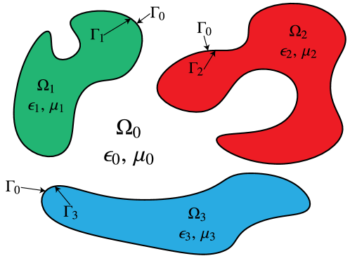
Figure 1: Boundary, domain, and material specifications for piecewise-constant geometries.

The generalized Debye source representation makes use of non-physical variables - using both potentials ($\vectorsym{A},\varphi$) and anti-potentials ($\vectorsym{Q},\psi$):

$$\vectorsym{E}_{\ell} =ik_{\ell}\vectorsym{A}_{\ell}-\nabla\varphi_{\ell}-\nabla\times\vectorsym{Q}_{\ell},$$ (2.6)

$$\vectorsym{H}_{\ell} =ik_{\ell}\vectorsym{Q}_{\ell}-\nabla\psi_{\ell}+\nabla\times\vectorsym{A}_{\ell},$$

where the potentials are given by

$$\vectorsym{A}_{\ell} =\mathcal{S}_{k_{\ell}}\vectorsym{J}_{\ell},\qquad \varphi_{\ell} =\mathcal{S}_{k_{\ell}}\rho_{\ell},$$ (2.7)

$$\vectorsym{Q}_{\ell} =\mathcal{S}_{k_{\ell}}\vectorsym{K}_{\ell}, \psi_{\ell} =\mathcal{S}_{k_{\ell}}\sigma_{\ell},$$

and the layer potentials $S_{k_{\ell}}$ are defined on the support of their argument. Thus,

$$\varphi_{\ell}(\vectorsym{x})=\int_{\Gamma_{\ell}}\frac{e^{ik|\vectorsym{x}-\vectorsym{x}^{\prime}|}}{4\pi|\vectorsym{x}-\vectorsym{x}^{\prime}|}\rho_{\ell}(\vectorsym{x}^{\prime})\,da(\vectorsym{x}^{\prime}),$$ (2.8)

with analogous expressions defining the other potentials in terms of their vector or scalar source densities ($\vectorsym{J}_{\ell},\vectorsym{K}_{\ell}$, and $\sigma_{\ell}$). Here, in a slight abuse of notation, $\rho$ is not the true electric charge, but a charge-like non-physical quantity. The tangential vector fields $\vectorsym{J}_{\ell}$, $\vectorsym{K}_{\ell}$ and the scalar functions $\rho_{\ell}$, $\sigma_{\ell}$ are defined on the boundary of the $\ell$th region $\Gamma_{\ell}$ (see Figure 1), and are responsible for representing the fields in the $\ell$th region. In order for Maxwell’s equations to be satisfied in a source-free region, the potentials must satisfy the relations $\nabla\cdot\vectorsym{A}_{\ell}=ik_{\ell}\varphi_{\ell}$ and $\nabla\cdot\vectorsym{Q}_{\ell}=ik_{\ell}\psi_{\ell}$. It is straightforward to show that this holds when the currents and charges satisfy the consistency conditions:

$$\nabla_{\Gamma_{\ell}}\cdot\vectorsym{J}_{\ell}=ik_{\ell}\rho_{\ell},\qquad\nabla_{\Gamma_{\ell}}\cdot\vectorsym{K}_{\ell}=ik_{\ell}\sigma_{\ell}.$$ (2.9)

Rather than using these conditions to define $\rho_{\ell},\sigma_{\ell}$, leading to catastrophic cancellation, or adding them as additional unknowns, requiring their imposition as additional constraints, we will construct $\vectorsym{J}_{\ell}$ and $\vectorsym{K}_{\ell}$ in such a way that (2.9) is automatically satisfied. That construction lies at the heart of the generalized Debye formalism, and the scalar surface densities $\rho_{\ell}$, $\sigma_{\ell}$ are referred to as generalized Debye sources. Thus, we define the currents $\vectorsym{J}_{\ell}$ and $\vectorsym{K}_{\ell}$ in terms of an explicit Hodge decomposition into divergence-free, curl-free, and harmonic components along each $\Gamma_{\ell}$:

$$\vectorsym{J}_{\ell} =\nabla_{\Gamma_{\ell}}\alpha_{J_{\ell}}+\vectorsym{{n}}\times\nabla_{\Gamma_{\ell}}\beta_{J_{\ell}}+\vectorsym{J}^{h}_{\ell},$$ (2.10)

$$\vectorsym{K}_{\ell} =\nabla_{\Gamma_{\ell}}\alpha_{K_{\ell}}+\vectorsym{{n}}\times\nabla_{\Gamma_{\ell}}\beta_{K_{\ell}}+\vectorsym{K}^{h}_{\ell},$$

where

$$\Delta_{\Gamma_{\ell}}\alpha_{J_{\ell}}=ik_{\ell}\rho_{\ell},\qquad\Delta_{\Gamma_{\ell}}\alpha_{K_{\ell}}=ik_{\ell}\sigma_{\ell},$$ (2.11)

$\nabla_{\Gamma_{\ell}}$ denotes the surface gradient, $\Delta_{\Gamma_{\ell}}$ denotes the surface Laplacian, and $\vectorsym{J}^{h}_{\ell}$, $\vectorsym{K}^{h}_{\ell}$ are harmonic vector fields on $\Gamma_{\ell}$. Recall that a tangential vector field $\vectorsym{L}$ is harmonic if it satisfies the conditions:

$$\nabla_{\Gamma_{\ell}}\cdot\vectorsym{L}=0,\qquad\nabla_{\Gamma_{\ell}}\cdot\vectorsym{{n}}\times\vectorsym{L}=0.$$ (2.12)

The dimension of the linear space of harmonic vector fields on each boundary component $\Gamma_{\ell}$ is simply $2g_{\ell}$, where $g_{\ell}$ is the genus of (the smooth) boundary $\Gamma_{\ell}$. Thus, we will write

$$\vectorsym{J}^{h}_{\ell}=\sum_{j=1}^{2g_{\ell}}a_{\ell j}\,\vectorsym{h}_{\ell j},\qquad\vectorsym{K}^{h}_{\ell}=\sum_{j=1}^{2g_{\ell}}b_{\ell j}\,\vectorsym{h}_{\ell j},$$ (2.13)

where the $\vectorsym{h}_{\ell j}$ form a basis for the harmonic vector fields. It is the coefficients $a_{\ell j}$, $b_{\ell j}$ that must be determined based on boundary data. It is important to note that the equations (2.11) guarantee that (2.9) is satisfied. One slight complication, addressed below, is that the sources $\rho_{\ell}$, $\sigma_{\ell}$ are required to be mean-zero, since the surface Laplacian is invertible only in the space of mean-zero functions [13]. Finally, $\beta_{J_{\ell}}$ and $\beta_{K_{\ell}}$ are chosen to be linear in $\rho_{\ell}$ and $\sigma_{\ell}$ in a manner that depends on the precise boundary conditions of interest.

For boundary-value problems in multiply-connected geometries, the generalized Debye approach requires a set of conditions to fix the harmonic components beyond the local boundary conditions imposed on the field quantities $\vectorsym{E}$, $\vectorsym{H}$. These (non-local) conditions are determined by considering $n_{g}=2\sum_{\ell}g_{\ell}$ separate line integrals of $\vectorsym{E}^{\textnormal{tot}}$, $\vectorsym{H}^{\textnormal{tot}}$ along loops contained in $\Gamma_{\ell}$ which enclose interior and exterior holes – that is to say, these loops $C_{1}$, …, $C_{n_{g}}$ must span the first homology group of $\Gamma_{\ell}.$ They take the general form:

$$\int_{C_{j}}\vectorsym{E}\cdot d\vectorsym{l}=f_{j},\quad\int_{C_{j}}\vectorsym{H}\cdot d\vectorsym{l}=g_{j},$$ (2.14)

for $j=1,\ldots,n_{g}$ and some set of constants $f_{j},g_{j}$. In scattering problems, the constants $f_{j},g_{j}$ usually correspond to some functional of the incoming fields and depend, again, on the particular boundary conditions. We will specify the precise constraints below for perfect conductors and dielectrics. See Figure 2 for an illustration of a possible set of loops $C_{j}$ in the genus 1 case.

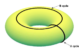
Figure 2: Loops spanning the interior and exterior homologies of a genus 1 surface.

Remark 1.

Since the generalized Debye construction enforces that the electric and magnetic fields satisfy the Maxwell equations, it can be used in applications which do not arise as scattering problems [16]. This is not true of many combined-field and charge-current representations, which work in the scattering setting only because the right-hand side is not arbitrary - it is derived from an incoming Maxwellian electromagnetic field (see, for example, [46]).

We now turn to the particular representation used for electromagnetic fields in the exterior of perfect conducting objects.

2.1 The perfect electric conductor (PEC)

We describe the generalized Debye representation for a single PEC object, since the extension to multiple objects is straightforward. Along the surface $\Gamma$ of $\Omega$ (a PEC), it is well known that

$$\vectorsym{{n}}\times\bm{{\mathcal{E}}}=\vectorsym{0},\qquad\vectorsym{{n}}\cdot\bm{\mathcal{H}}=0.$$ (2.15)

In the case of scattering from a PEC, the current-like vector fields $\vectorsym{J}$ and $\vectorsym{K}$ in the generalized Debye source representation can be constructed as [13]:

$$\vectorsym{J} =ik\left(\nabla_{\Gamma}\Delta_{\Gamma}^{-1}\rho-\vectorsym{{n}}\times\nabla_{\Gamma}\Delta_{\Gamma}^{-1}\sigma\right)+\vectorsym{J}^{h},$$ (2.16)

$$\vectorsym{K} =\vectorsym{{n}}\times\vectorsym{J}.$$

Here, $\Delta_{\Gamma}^{-1}$ denotes the inverse of the Laplace-Beltrami operator (the surface Laplacian) along $\Gamma$ restricted to mean-zero functions. On the space of mean-zero functions defined along $\Gamma$, this operator is uniquely invertible. Using this construction for $\vectorsym{J}$ and $\vectorsym{K}$ and enforcing the preconditioned [37] homogeneous boundary conditions

$$\mathcal{S}_{0}\nabla_{\Gamma}\cdot\vectorsym{E}^{\textnormal{tot}} =0, \text{on }\Gamma,$$ (2.17)

$$\vectorsym{{n}}\cdot\vectorsym{H}^{\textnormal{tot}} =0, \text{on }\Gamma,$$

$$\int_{C_{j}}\vectorsym{E}^{\textnormal{tot}}\cdot d\vectorsym{l} =0, \text{for }j=1,\ldots,2g$$

yields a second-kind integral equation for $\rho$, $\sigma$, and $\vectorsym{J}^{h}=\sum_{j=1}^{2g_{\ell}}a_{j}\,\vectorsym{h}_{j}$ which is uniquely invertible for all values of $k$ with non-negative imaginary part [13]. By construction, the scattered fields automatically satisfy the Silver-Müller radiation conditions at infinity. Here $\mathcal{S}_{0}$ is the zero-frequency single-layer potential operator. The system in (2.17) can be written more explicitly as:

$$\frac{1}{4}\rho+\mathcal{K}_{E}[\rho,\sigma,a_{j}] =-\mathcal{S}_{0}\nabla_{\Gamma}\cdot\vectorsym{E}^{\textnormal{in}}, \text{on }\Gamma,$$ (2.18)

$$\frac{1}{2}\sigma+\mathcal{K}_{H}[\rho,\sigma,a_{j}] =-\vectorsym{{n}}\cdot\vectorsym{H}^{\textnormal{in}}, \text{on }\Gamma,$$

$$\int_{C_{j}}\vectorsym{E}^{\textnormal{tot}}\cdot d\vectorsym{l} =0, \text{for }j=1,\ldots,2g,$$

with the operators $\mathcal{K}_{E}$ and $\mathcal{K}_{H}$ given by

$$\mathcal{K}_{E}[\rho,\sigma,a_{j}] =ik\mathcal{S}_{0}\nabla_{\Gamma}\cdot\mathcal{S}_{k}\vectorsym{J}-\mathcal{C}_{k}\rho-\mathcal{S}_{0}\nabla_{\Gamma}\cdot\nabla\times\mathcal{S}_{k}\vectorsym{K},$$ (2.19)

$$\mathcal{K}_{H}[\rho,\sigma,a_{j}] =ik\vectorsym{{n}}\cdot\mathcal{S}_{k}\vectorsym{K}-\mathcal{S}^{\prime}_{k}\sigma+\vectorsym{{n}}\cdot\nabla\times\mathcal{S}_{k}\vectorsym{J},$$

where

$$\mathcal{S}_{k}^{\prime}f(\vectorsym{x})=\frac{\partial}{\partial n}\int_{\Gamma}G(\vectorsym{x},\vectorsym{x}^{\prime})\,f(\vectorsym{x})\,da(\vectorsym{x}^{\prime}),$$ (2.20)

with $\partial/\partial n$ denoting differentiation in the direction normal to $\Gamma$ at $\vectorsym{x}$ and $G$ denoting the Green’s function for the Helmholtz equation:

$$G(\vectorsym{x},\vectorsym{x}^{\prime})=\frac{e^{ik|\vectorsym{x}-\vectorsym{x}^{\prime}|}}{4\pi|\vectorsym{x}-\vectorsym{x}^{\prime}|}.$$ (2.21)

The operator $\mathcal{C}_{k}$ denotes the principal value part of the operator $\mathcal{S}_{0}\Delta_{\Gamma}\mathcal{S}_{k}$, given by:

$$\mathcal{C}_{k}f(\vectorsym{x}) =\text{p.v. }\int_{\Gamma}\frac{1}{4\pi|\vectorsym{x}-\vectorsym{x}^{\prime}|}\nabla_{\Gamma}\cdot\nabla_{\Gamma}\int_{\Gamma}G(\vectorsym{x}^{\prime},\vectorsym{x}^{\prime\prime})f(\vectorsym{x}^{\prime\prime})\,da(\vectorsym{x}^{\prime\prime})\,da(\vectorsym{x}^{\prime})$$ (2.22)

$$=-\text{p.v. }\int_{\Gamma}\nabla_{\Gamma}^{\prime}\frac{1}{4\pi|\vectorsym{x}-\vectorsym{x}^{\prime}|}\cdot\int_{\Gamma}\nabla_{\Gamma}^{\prime}G(\vectorsym{x}^{\prime},\vectorsym{x}^{\prime\prime})f(\vectorsym{x}^{\prime\prime})\,da(\vectorsym{x}^{\prime\prime})\,da(\vectorsym{x}^{\prime}),$$

where $\nabla_{\Gamma}^{\prime}$ denotes the surface gradient in the $\vectorsym{x}^{\prime}$ variable. See [39] for a computation of a similar operator, $\mathcal{S}_{0}\Delta_{\Gamma}\mathcal{S}_{0}$ using Caldéron projectors.

In the above expression, for simplicity reasons, the dependence of $\vectorsym{J}$ and $\vectorsym{K}$ on the variables $\rho$ and $\sigma$ and the coefficients $a_{j}$ has been suppressed. All integral operators above are interpreted in their on-surface principal-value sense. It is worth pointing out that the third terms in $\mathcal{K}_{E}$ and $\mathcal{K}_{H}$ are in fact order-zero operators with respect to the quantities $\vectorsym{J}$ and $\vectorsym{K}$. They are of order minus-one with regard to the variables $\rho$ and $\sigma$, as can be seen from the construction of $\vectorsym{J}$ and $\vectorsym{K}$.

Remark 2.

The system of integral equations in (2.17) is uniquely invertible with the restriction that $\rho$, $\sigma$ (the generalized Debye sources) and the data are all mean-zero functions. Without explicitly enforcing this condition the system is rank-one deficient, as can be seen from the operator $\mathcal{S}_{0}\Delta_{\Gamma}\mathcal{S}_{k}$ (which has a null-space of rank one). In Section 4.5 we show how to incorporate this constraint as a rank-one update to the system matrix [43].

2.2 Dielectric bodies

If the object $\Omega$ is not perfectly conducting, but rather made of a dielectric material [28], then the interfaces between regions do not support physical current or charge sheets. The materials merely become polarized, without the flow of charge, resulting in conditions at interfaces based on continuity of the normal and tangential components of the electric and magnetic fields. These boundary conditions can be written as:

$$\left[\vectorsym{n}\times\bm{{\mathcal{E}}}\right] =0, \qquad\left[\vectorsym{n}\cdot\epsilon\bm{{\mathcal{E}}}\right] =0,$$ (2.23)

$$\left[\vectorsym{n}\times\bm{\mathcal{H}}\right] =0, \left[\vectorsym{n}\cdot\mu\bm{\mathcal{H}}\right] =0.$$

Recall that the quantities $\bm{{\mathcal{D}}}=\epsilon\bm{{\mathcal{E}}}$ and $\bm{{\mathcal{B}}}=\mu\bm{\mathcal{H}}$ are the electric displacement and magnetic induction vector fields, respectively; it is these fields whose normal components are continuous across interfaces [41].

As in (2.6), we can use the generalized Debye source representation to construct $\vectorsym{E}$, $\vectorsym{H}$ in each dielectric region using layer potentials supported on the interface [15]:

$$\vectorsym{E}_{\ell} =\sqrt{\epsilon_{\ell}\mu_{\ell}}\left(ik_{\ell}\vectorsym{A}_{\ell}-\nabla\varphi_{\ell}-\nabla\times\vectorsym{Q}_{\ell}\right),$$ (2.24)

$$\vectorsym{H}_{\ell} =\sqrt{\epsilon_{\ell}\mu_{\ell}}\left(ik_{\ell}\vectorsym{Q}_{\ell}-\nabla\psi_{\ell}+\nabla\times\vectorsym{A}_{\ell}\right).$$

Along the boundary of each dielectric region $\Omega_{\ell}$ we define tangential vector fields $\vectorsym{J}_{\ell}$, $\vectorsym{K}_{\ell}$ which will be constructed to automatically satisfy the continuity conditions:

$$\nabla_{\Gamma_{\ell}}\cdot\vectorsym{J}_{\ell}=ik_{\ell}\rho_{\ell},\qquad\nabla_{\Gamma_{\ell}}\cdot\vectorsym{K}_{\ell}=ik_{\ell}\sigma_{\ell}.$$ (2.25)

Let us denote by $\rho_{\ell^{\prime}}$, $\sigma_{\ell^{\prime}}$ the generalized Debye sources supported on the opposite side of $\Gamma_{\ell}$ (i.e. those generalized Debye sources which are responsible for generating fields in region $\ell^{\prime}$). Then, as shown in [15], the following construction of $\vectorsym{J}_{\ell}$, $\vectorsym{K}_{\ell}$ leads to a uniquely invertible system of second-kind integral equations. We describe the construction in the case of only one component, $\Omega_{1}$, as it simplifies things greatly. The case of multiple components (and nested components) extends straightforwardly and is detailed in [15]. To this end, define the currents along $\Gamma_{0}$ by:

$$\vectorsym{J}_{0} =i\omega\left(\sqrt{\epsilon_{0}\mu_{0}}\nabla_{\Gamma}\Delta_{\Gamma}^{-1}\rho_{0}-\vectorsym{n}\times\epsilon_{1}\sqrt{\frac{\mu_{1}}{\epsilon_{0}}}\nabla_{\Gamma}\Delta_{\Gamma}^{-1}\rho_{1}\right)+\vectorsym{J}_{0}^{h},$$ (2.26)

$$\vectorsym{K}_{0} =i\omega\left(\sqrt{\epsilon_{1}\mu_{1}}\nabla_{\Gamma}\Delta_{\Gamma}^{-1}\sigma_{0}-\vectorsym{n}\times\mu_{1}\sqrt{\frac{\epsilon_{1}}{\mu_{0}}}\nabla_{\Gamma}\Delta_{\Gamma}^{-1}\sigma_{1}\right)+\vectorsym{K}_{0}^{h},$$

with the (unrelated) harmonic components given by:

$$\vectorsym{J}_{0}^{h}=\sum_{j=1}^{2g}a_{j}\vectorsym{h}_{j},\qquad\vectorsym{K}_{0}^{h}=\sum_{j=1}^{2g}b_{j}\vectorsym{h}_{j},$$ (2.27)

where $g$ denotes the genus of $\Gamma_{0}=\Gamma_{1}$. The Debye currents $\vectorsym{J}_{1}$, $\vectorsym{K}_{1}$ defining vector potentials in the interior domain, $\Omega_{1}$, are then linearly related to the currents $\vectorsym{J}_{0}$ and $\vectorsym{K}_{0}$, similar to the classic Muller integral equation [36]. Acting on tangential vector fields along a boundary $\Gamma$, given in their Hodge decomposition, let the linear operator $\mathcal{U}$ be defined as:

$$\vectorsym{F} =\nabla_{\Gamma}\alpha+\vectorsym{n}\times\nabla_{\Gamma}\beta+\vectorsym{h},$$ (2.28)

$$\mathcal{U}\vectorsym{F} =-\nabla_{\Gamma}\beta+\vectorsym{n}\times\nabla_{\Gamma}\alpha+\vectorsym{h}.$$

The operator $\mathcal{U}$ is known as the clutching map [15], and is equivalent to $\mathcal{U}=\mathcal{I}$ when acting on harmonic components and $\mathcal{U}=\vectorsym{n}\times$ when acting on the complement of the space of harmonic vector fields. The interior Debye currents, $\vectorsym{J}_{1}$, $\vectorsym{K}_{1}$, are then given as

$$\vectorsym{J}_{1}=\sqrt{\frac{\epsilon_{0}}{\epsilon_{1}}}\mathcal{U}\vectorsym{J}_{0},\qquad\vectorsym{K}_{1}=\sqrt{\frac{\mu_{0}}{\mu_{1}}}\mathcal{U}\vectorsym{K}_{0}.$$ (2.29)

This construction ensures uniqueness in the resulting integral equations.

It is important to note that by convention, we assume that $\Gamma_{\ell}$ and $\Gamma_{\ell^{\prime}}$ are oriented in the same manner, i.e. that the unit normal vector along the boundary always points into $\Omega_{0}$, the unbounded component of $\mathbb{R}^{3}$. Other conventions would merely result in a change in some of the signs in the above formulas. Also, note that our indexing of regions is opposite that from [15]. Here, we denote the outermost unbounded region by $\Omega_{0}$, as is standard in the computational electromagnetics literature.

Next, as shown in [15], the following boundary conditions lead to a system of second-kind integral equations that are uniquely invertible for all $\omega$, including in the limit as $\omega\to 0$:

$$\mathcal{S}_{0}\nabla_{\Gamma}\cdot\left[\vectorsym{E}^{\textnormal{tot}}\right] =0,$$ (2.30)

$$\mathcal{S}_{0}\nabla_{\Gamma}\cdot\left[\vectorsym{H}^{\textnormal{tot}}\right] =0,$$

$$\left[\vectorsym{n}\cdot\sqrt{\epsilon}\vectorsym{E}^{\textnormal{tot}}\right] =0,$$

$$\left[\vectorsym{n}\cdot\sqrt{\mu}\vectorsym{H}^{\textnormal{tot}}\right] =0, \text{on }\Gamma,$$

$$\int_{C_{j}}\left[\vectorsym{E}^{\textnormal{tot}}\right]\cdot d\vectorsym{l} =0,$$

$$\int_{C_{j}}\left[\vectorsym{H}^{\textnormal{tot}}\right]\cdot d\vectorsym{l} =0, \text{for }j=1,\ldots,2n_{g},$$

where the contours $C_{j}$, as before, span the space of the first homology group in $\mathbb{R}^{3}\setminus\Omega$ and $\Omega$. The above system uniquely determines $\rho_{\ell}$, $\sigma_{\ell}$, $\vectorsym{J}_{\ell}^{h}$, and $\vectorsym{K}_{\ell}^{h}$. The system can be expanded as in Section 2.1; we omit such an expansion here for clarity as there are no new operators introduced. However, it is worth pointing out that, in what follows, we will always assume that the incoming electromagnetic fields $\vectorsym{E}^{\textnormal{in}}$, $\vectorsym{H}^{\textnormal{in}}$ are generated only from sources located in $\Omega_{0}$. In the case of the electric field and one component, the interface conditions take the same form as before:

$$\mathcal{S}_{0}\nabla_{\Gamma}\cdot\left(\vectorsym{E}_{0}-\vectorsym{E}_{1}\right) =-\mathcal{S}_{0}\nabla_{\Gamma}\cdot\vectorsym{E}^{\textnormal{in}}$$ (2.31)

$$\vectorsym{n}\cdot\left(\sqrt{\epsilon_{0}}\vectorsym{E}_{0}-\sqrt{\epsilon_{1}}\vectorsym{E}_{1}\right) =-\vectorsym{n}\cdot\sqrt{\epsilon_{0}}\vectorsym{E}^{\textnormal{in}}.$$

The jump conditions on the magnetic field are analogous.

In the next section, we turn to a description of a separation of variables, FFT-accelerated solver for the PEC system (2.18) and dielectric system (2.30) in the case of a single component, $\Omega$, assuming it is a body of revolution.

3 Integral equations on surfaces of revolution

The numerical solution of boundary integral equations on general smooth surfaces in three dimensions has been an active area of research for several decades, but robust, efficient and high-order accurate solvers are not easy to develop, mainly due to issues of surface representation and quadrature. However, when the geometry contains rotational symmetry about, say, the $z$-axis, separation of variables and Fourier decomposition can be used to turn the problem into a sequence of boundary integral equations along a one-dimensional curve, for which many fast and accurate numerical methods exist.

3.1 Geometry

In this section we establish the coordinate system to be used for a surface of revolution $\Gamma$, describe the corresponding Fourier analysis, and discuss the form taken by surface differential operators. The scalar case has been carefully treated in [51, 25], which we extend here to the vector-valued case. A special case of the present analysis, focusing on purely axisymmetric solutions with applications to magnetohydrodynamics (MHD), was recently presented in [40].

We denote the usual unit vector basis in Cartesian coordinates as $\{\vectorsym{{i}},\vectorsym{{j}},\vectorsym{{k}}\}$ and the usual unit vector basis in cylindrical coordinates as $\{\vectorsym{{r}},{\vectorsym{{\theta}}},\vectorsym{{k}}\}$:

$$\vectorsym{{r}}(\theta) =\cos\theta\,\vectorsym{{i}}+\sin\theta\,\vectorsym{{j}} \qquad\vectorsym{{i}} =\cos\theta\,\vectorsym{{r}}(\theta)-\sin\theta\,{\vectorsym{{\theta}}}(\theta)$$ (3.1)

$${\vectorsym{{\theta}}}(\theta) =-\sin\theta\,\vectorsym{{i}}+\cos\theta\,\vectorsym{{j}} \qquad\vectorsym{{j}} =\sin\theta\,\vectorsym{{r}}(\theta)+\cos\theta\,{\vectorsym{{\theta}}}(\theta)$$

where we have given formulae for both cylindrical and Cartesian unit vectors in terms of the other. These relationships will be useful in the following sections. The following addition formulae will also be useful:

$$\vectorsym{{r}}(\theta-\varphi) =\cos\varphi\,\vectorsym{{r}}(\theta)-\sin\varphi\,{\vectorsym{{\theta}}}(\theta)$$ (3.2)

$${\vectorsym{{\theta}}}(\theta-\varphi) =\sin\varphi\,\vectorsym{{r}}(\theta)+\cos\varphi\,{\vectorsym{{\theta}}}(\theta)$$

We will omit the implicit dependence (relative to $\vectorsym{{i}}$ and $\vectorsym{{j}}$) of $\vectorsym{{r}}$ and ${\vectorsym{{\theta}}}$ on the variable $\theta$ from now on, unless it is explicitly required. In order to avoid confusion going forward, targets will usually be denoted by $\vectorsym{x}$ and sources will usually be denoted by $\vectorsym{x}^{\prime}$. This notation will be consistent with integrating variables as well (integrals will be performed in $r^{\prime}$, $\theta^{\prime}$, and $z^{\prime}$ variables).

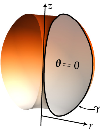
(a) The generating curve $\vectorsym{\gamma}$.

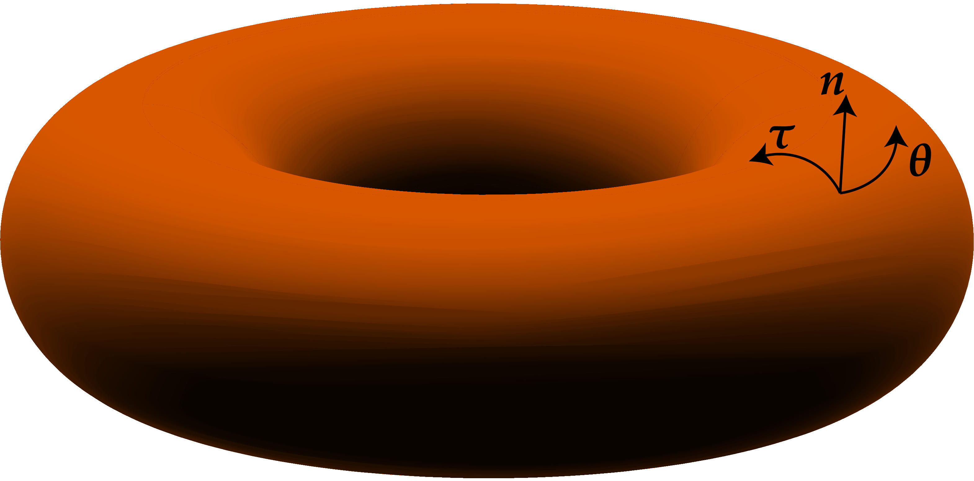
(b) A local system of coordinates along $\Gamma$.

Figure 3: Geometry of a body of revolution.

Let the smooth closed curve $\vectorsym{\gamma}:[0,L]\to\mathbb{R}^{3}$ be contained in the $\theta=0$ plane, and let points on this curve be parameterized in arclength as

$$\vectorsym{\gamma}(s)=\left(r(s),0,z(s)\right),$$ (3.3)

in cylindrical coordinates. The boundary $\Gamma$ of a body of revolution $\Omega$ is then generated by rotating $\vectorsym{\gamma}$ about the $z$-axis. A local orthonormal basis along $\Gamma$ (assuming that $\vectorsym{\gamma}$ is oriented counter-clockwise) will be denoted by $\{\vectorsym{{\tau}},{\vectorsym{{\theta}}},\vectorsym{{n}}\}$ with ${\vectorsym{{\theta}}}$ the usual cylindrical coordinate unit vector and

$$\vectorsym{{\tau}} =\frac{dr}{ds}\,\vectorsym{{r}}+\frac{dz}{ds}\,\vectorsym{{k}},$$ (3.4)

$$\vectorsym{{n}} ={\vectorsym{{\theta}}}\times\vectorsym{{\tau}}.$$

See Figure 3 for a depiction of the setup and relevant coordinate system.

Lastly, we note that along a surface of revolution of genus 1 (i.e. a toroidal surface), the harmonic vector fields discussed in Section 2 are known analytically and given by

$$\vectorsym{h}_{1}=\frac{1}{r}\vectorsym{{\tau}},\qquad\vectorsym{h}_{2}=-\frac{1}{r}{\vectorsym{{\theta}}}.$$ (3.5)

3.2 The scalar function case

Scalar-valued boundary integral equations on surfaces of revolution can be Fourier decomposed straightforwardly, as in [51, 25]. We briefly state the decomposition here, and then discuss the vector-valued case in detail.

Along the boundary $\Gamma$ of a body of revolution, a second-kind integral equation with translation invariant kernel $G$ takes the form:

$$\sigma(\vectorsym{x})+\int_{\Gamma}G(\vectorsym{x}-\vectorsym{x}^{\prime})\,\sigma(\vectorsym{x}^{\prime})\,da(\vectorsym{x}^{\prime})=f(\vectorsym{x}),$$ (3.6)

for $\vectorsym{x}\in\Gamma$ and $da(\vectorsym{x}^{\prime})=r^{\prime}\,d\theta^{\prime}\,ds^{\prime}$. Since $G$ is assumed to be translation invariant, this means that $G$, in particular, is rotationally invariant: $G(\vectorsym{x}-\vectorsym{x}^{\prime})=G(r,z,r^{\prime},z^{\prime},\theta-\theta^{\prime})$. Expanding the solution $\sigma$ and right-hand side $f$ in terms of their Fourier series in the azimuthal direction $\theta$, we have:

$$\sigma(s,\theta)=\sum_{m=-\infty}^{\infty}\sigma_{m}(s)\,e^{im\theta},\qquad f(s,\theta)=\sum_{m=-\infty}^{\infty}f_{m}(s)\,e^{im\theta},$$ (3.7)

where the Fourier coefficient functions $\sigma_{m}$ and $f_{m}$ are given by

$$\sigma_{m}(s)=\frac{1}{2\pi}\int_{-\pi}^{\pi}\sigma(s,\theta)\,e^{-im\theta}\,d\theta,\qquad f_{m}(s)=\frac{1}{2\pi}\int_{-\pi}^{\pi}f(s,\theta)\,e^{-im\theta}\,d\theta.$$ (3.8)

Substituting the Fourier representations for $\sigma$ and $f$ in (3.7) into the integral equation in (3.6), and collecting terms mode-by-mode, we have the following decoupled integral equations along the generating curve $\vectorsym{\gamma}$:

$$\sigma_{m}(s)+\int_{\gamma}\sigma_{m}(s^{\prime})\int_{-\pi}^{\pi}G(s,s^{\prime},\theta-\theta^{\prime})\,e^{-im\theta^{\prime}}\,r^{\prime}\,d\theta^{\prime}\,ds^{\prime}=f_{m}(s),\\ \implies\quad\sigma_{m}(s)+2\pi\int_{\gamma}G_{m}(s,s^{\prime})\,\sigma_{m}(s^{\prime})\,r^{\prime}\,ds^{\prime}=f_{m}(s)$$ (3.9)

for all $m$, where we denote the Fourier modes of $G$ as $G_{m}$:

$$G(r,z,r^{\prime},z^{\prime},\theta-\theta^{\prime})=\sum_{m=-\infty}^{\infty}G_{m}(r,z,r^{\prime},z^{\prime})\,e^{im(\theta-\theta^{\prime})}\\ \iff\quad G_{m}(r,z,r^{\prime},z^{\prime})=\frac{1}{2\pi}\int_{-\pi}^{\pi}G(r,z,r^{\prime},z^{\prime},\varphi)\,e^{-im\varphi}\,d\varphi.$$ (3.10)

We use the notation $G(s,s^{\prime},\theta-\theta^{\prime})=G(\vectorsym{x}-\vectorsym{x}^{\prime})$ when both $\vectorsym{x}$ and $\vectorsym{x}^{\prime}$ are located on $\Gamma$, and likewise for the Fourier modes $G_{m}$. This separation of variables procedure has reduced the problem of solving a boundary integral equation on a surface embedded in three dimensions to that of solving a sequence of boundary integral equations along the curve $\gamma$, which is embedded in two dimensions. Given an efficient method for evaluating the modal Green’s functions $G_{m}$, performing the synthesis and analysis of $\sigma$ and $f$ using the Fast Fourier Transform (FFT) [6] yields a very efficient direct solver for the original problem. The efficient evaluation of $G_{m}$, for both the Laplace and Helmholtz problems, is a long-studied problem and discussed in Section 4.2.

We now turn our attention to an analogous problem, that of Fourier decomposing a vector-valued integral equation along a surface of revolution. While the generalized Debye system in (2.18) is defined in terms of scalar-valued unknowns, its discretization requires the application of layer potential operators to vector quantities. Slightly more care is required than in the scalar case.

3.3 The vector-valued case

As in the scalar case, a second-kind vector-valued boundary integral equation with translation invariant kernel $G$ is of the form:

$$\vectorsym{u}(\vectorsym{x})+\int_{\Gamma}G(\vectorsym{x},\vectorsym{x}^{\prime})\,\vectorsym{u}(\vectorsym{x}^{\prime})\,da(\vectorsym{x}^{\prime})=\vectorsym{f}(\vectorsym{x}).$$ (3.11)

In the electromagnetic setting, both $\vectorsym{u}$ and $\bm{f}$ are typically tangential vector fields, so we address that case only. Fully three-dimensional surface vector fields are encountered in fluid dynamics and elasticity, and many of the following calculations extend directly to those problems, albeit with components lying in the direction normal to $\Gamma$ as well.

Since $\Gamma$ is a surface of revolution, the tangential vector fields in (3.11) can be written in terms of their Fourier series, component-wise, with respect to the local basis $\vectorsym{{\tau}}$, ${\vectorsym{{\theta}}}$:

$$\vectorsym{u}(s,\theta) =\sum_{m}\left(u_{\tau,m}(s)\,\vectorsym{{\tau}}+u_{\theta,m}(s)\,{\vectorsym{{\theta}}}\right)e^{im\theta},$$ (3.12)

$$\vectorsym{f}(s,\theta) =\sum_{m}\left(f_{\tau,m}(s)\,\vectorsym{{\tau}}+f_{\theta,m}(s)\,{\vectorsym{{\theta}}}\right)e^{im\theta}.$$

Assuming that $\vectorsym{f}$ is square-integrable along $\Gamma$, and that (3.11) is a Fredholm second-kind integral equation, it can be shown that the solution $\vectorsym{u}$ is also square integrable [3]. Therefore, the Fourier representations in (3.12) are complete. Since we have that $G$ is rotationally invariant, plugging the Fourier expansion for $\vectorsym{u}$ into the integral term in (3.11) we have:

$$\int_{\Gamma}G(\vectorsym{x}-\vectorsym{x}^{\prime})\,\vectorsym{u}(\vectorsym{x}^{\prime})\,da(\vectorsym{x}^{\prime})\\ =\int_{\gamma}\int_{-\pi}^{\pi}G(s,s^{\prime},\theta-\theta^{\prime})\sum_{m}\left(u_{\tau,m}(s^{\prime})\,\vectorsym{{\tau}}(s^{\prime},\theta^{\prime})+u_{\theta,m}(s^{\prime})\,{\vectorsym{{\theta}}}(\theta^{\prime})\right)e^{im\theta^{\prime}}\,r^{\prime}d\theta^{\prime}\,ds^{\prime}.$$ (3.13)

We now calculate the projection of this integral onto the $m$th Fourier mode with respect to the unit vectors $\vectorsym{{r}}(\theta)$, ${\vectorsym{{\theta}}}(\theta)$. The unit vectors $\vectorsym{{r}}(\theta^{\prime})$ and ${\vectorsym{{\theta}}}(\theta^{\prime})$ cannot be pulled outside of the integrals, however it is a direct consequence of the addition formulas in equation (3.2) that:

$$\int_{-\pi}^{\pi}G(\cdot,\theta-\theta^{\prime})\,\vectorsym{{r}}(\theta^{\prime})\,e^{im\theta^{\prime}}\,d\theta^{\prime} =e^{im\theta}\int_{-\pi}^{\pi}G(\cdot,\varphi)\,\vectorsym{{r}}(\theta-\varphi)\,e^{-im\varphi}\,d\varphi$$ (3.14)

$$=e^{im\theta}\,\vectorsym{{r}}(\theta)\int_{-\pi}^{\pi}G(\cdot,\varphi)\,\cos\varphi\,e^{-im\varphi}\,d\varphi$$

$$\qquad-e^{im\theta}\,{\vectorsym{{\theta}}}(\theta)\int_{-\pi}^{\pi}G(\cdot,\varphi)\,\sin\varphi\,e^{-im\varphi}\,d\varphi$$

$$=e^{im\theta}\left(G_{m}^{\cos}(\cdot)\,\vectorsym{{r}}(\theta)-G_{m}^{\sin}(\cdot)\,{\vectorsym{{\theta}}}(\theta)\right)$$

where

$$G_{m}^{\cos}(\cdot) =\int_{-\pi}^{\pi}G(\cdot,\varphi)\,\cos\varphi\,e^{-im\varphi}\,d\varphi,$$ (3.15)

$$G_{m}^{\sin}(\cdot) =\int_{-\pi}^{\pi}G(\cdot,\varphi)\,\sin\varphi\,e^{-im\varphi}\,d\varphi.$$

Likewise, we have that

$$\int_{-\pi}^{\pi}G(\cdot,\theta-\theta^{\prime})\,{\vectorsym{{\theta}}}(\theta^{\prime})\,e^{im\theta^{\prime}}\,d\theta^{\prime}=e^{im\theta}\left(G_{m}^{\sin}(\cdot)\,\vectorsym{{r}}(\theta)+G_{m}^{\cos}(\cdot)\,{\vectorsym{{\theta}}}(\theta)\right).$$ (3.16)

Recalling that $\vectorsym{{\tau}}=\frac{dr}{ds}\vectorsym{{r}}+\frac{dz}{ds}\vectorsym{{k}}$, the integral equation in (3.11) can be re-written mode by mode for all $m$, and component-wise as:

$$\vectorsym{{r}} : \quad u_{\tau,m}\,\frac{dr}{ds}+\int_{\gamma}\left(G^{\cos}_{m}(\cdot,s^{\prime})\,\frac{dr}{ds^{\prime}}\,u_{\tau,m}+G^{\sin}_{m}(\cdot,s^{\prime})\,u_{\theta,m}\right)\,r^{\prime}\,ds^{\prime} =\frac{dr}{ds}\,f_{\tau,m},$$ (3.17)

$${\vectorsym{{\theta}}} : u_{\theta,m}+\int_{\gamma}\left(G^{\cos}_{m}(\cdot,s^{\prime})\,u_{\theta,m}-G^{\sin}_{m}(\cdot,s^{\prime})\,u_{\tau,m}\,\frac{dr}{ds^{\prime}}\right)\,r^{\prime}\,ds^{\prime} =f_{\theta,m},$$

$$\vectorsym{{k}} : u_{\tau,m}\,\frac{dz}{ds}+\int_{\gamma}G_{m}(\cdot,s^{\prime})\,\frac{dz}{ds^{\prime}}\,u_{\tau,m}\,r^{\prime}\,ds^{\prime} =\frac{dz}{ds}\,f_{\tau,m}.$$

The previous integral equations, while decoupled with respect to Fourier mode $m$ and cylindrical coordinate vector components $\vectorsym{{r}}$, ${\vectorsym{{\theta}}}$, $\vectorsym{{k}}$, are not decoupled with respect to the components of $\vectorsym{u}$, $u_{\tau,m}$ and $u_{\theta,m}$. This is due to the action of the integral operator on the local coordinate system, $\vectorsym{{\tau}}$, ${\vectorsym{{\theta}}}$, $\vectorsym{{n}}$. Depending on the exact boundary conditions, linear combinations of the above integral equations may be taken to form an even more coupled, second-kind system (since it is obvious that one could solve for $u_{\tau,m}$ first, and then for $u_{\theta,m}$). The main point here is to demonstrate that the vector-value case is more involved than the scalar case, and that there are additional kernels that need to be evaluated: $G_{m}^{\cos}$ and $G_{m}^{\sin}$. Furthermore, the integral equations that we will actually be discretizing involve the composition of layer potential operators. This case can be handled analogously.

3.4 Surface differentials

The integral equations resulting from the generalized Debye representations make explicit use of the Hodge decomposition of tangential vector fields, and therefore require the application of surface differential operators. In this section we briefly give formulae for these operators along the axisymmetric boundary $\Gamma$: the surface gradient $\nabla_{\Gamma}$, the surface divergence $\nabla_{\Gamma}\cdot$, and the surface Laplacian $\Delta_{\Gamma}$. Furthermore, the construction of surface currents $\vectorsym{J}$ and $\vectorsym{K}$ requires the application of $\Delta_{\Gamma}^{-1}$. We provide the formula for $\Delta_{\Gamma}$ below, and then in Section 4.3 discuss a numerical method for inverting it. In order to somewhat simplify the resulting expressions, we assume that the generating curve $\gamma$ of the boundary $\Gamma$ is parameterized by arclength $s$. Similar formulae with arbitrary parameterizations or curvilinear coordinates can be found in most differential geometry or mathematical physics texts, see for example [37, 18].

Let $f(s,\theta)=g(s)\,e^{im\theta}$ be a scalar function defined on $\Gamma$ and

$$\vectorsym{F}(s,\theta)=(F_{\tau}(s)\,\vectorsym{\tau}+F_{\theta}(s)\,\vectorsym{\theta})\,e^{im\theta}$$

be a vector field tangential to $\Gamma$. We then have the following three expressions for the surface differentials:

$$\begin{gathered}\nabla_{\Gamma,m}f=\frac{\partial f}{\partial s}\,\vectorsym{\tau}+\frac{im}{r}f\,\vectorsym{\theta},\\ \nabla_{\Gamma,m}\cdot\vectorsym{F}=\frac{\partial F_{\tau}}{\partial s}+\frac{1}{r}\frac{\partial r}{\partial s}F_{\tau}+\frac{im}{r}F_{\theta},\\ \Delta_{\Gamma,m}f=\frac{\partial^{2}f}{\partial s^{2}}+\frac{1}{r}\frac{\partial r}{\partial s}\frac{\partial f}{\partial s}-\frac{m^{2}}{r^{2}}f.\end{gathered}$$ (3.18)

The on-surface quantity $\nabla\times\vectorsym{F}$, where $\nabla\times$ denotes the three-dimensional curl operator, can be computed for the tangential $\vectorsym{F}$ above by using the standard curl in cylindrical coordinates along with the relationships:

$$\vectorsym{{r}}=\frac{dr}{ds}\vectorsym{{\tau}}+\frac{dz}{ds}\vectorsym{{n}},\qquad\vectorsym{{k}}=\frac{dz}{ds}\vectorsym{{\tau}}-\frac{dr}{ds}\vectorsym{{n}}.\\$$ (3.19)

4 A high-order solver

In this section we detail the various parts of the solver, including the efficient numerical evaluation of the modal Green’s functions, application of the surface differentials, inversion of the surface Laplacian, and stable evaluation of the auxiliary boundary conditions required by the Debye formulation. The resulting linear systems, one for each Fourier mode, are then solved directly using LAPACK’s dense LU routines. This part of the computation is not a dominant one, so no large effort was made to accelerate it. First, we describe the Nyström discretization of the integral equation.

4.1 Nyström discretization

We restrict our examples in this work to integral equations along smooth boundaries $\Gamma$ of genus one. As a consequence, the generating curve $\gamma$, is represented by a smooth periodic, $\mathbb{R}^{2}$-valued function. The resulting integral equations along $\gamma$ are discretized at equispaced points, and the resulting weakly-singular quadrature is performed using hybrid Gauss-Trapezoidal quadratures [2]. These quadrature rules are designed for logarithmic singularities; while the fully three-dimensional Green’s function for the Helmholtz equation has a $1/r$ singularity, each of the modal Green’s functions only has a logarithmic singularity (as can be seen from their special function representations [8, 11]), and therefore high-order accuracy can be obtained using these rules. A thorough discussion of these quadrature rules, and Nyström discretization in general, is contained in [24], along with a comparison with other methods. Using this discretization method, a continuous integral equation of the form

$$\sigma(s)+\int_{\gamma}K(s,s^{\prime})\,\sigma(s^{\prime})\,ds^{\prime}=f(s),$$ (4.1)

is approximated by the finite dimensional system

$$\sigma_{j}+\frac{2\pi L}{N}\sum_{k\neq j}w_{jk}\,K(s_{j},s_{k})\,\sigma_{k}=f(s_{j}),\qquad\text{for }j=1,\ldots,N,$$ (4.2)

where $L$ is the length of $\gamma$, the $w_{jk}$ are the quadrature weights for the Gauss-Trapezoidal rule, and $\sigma_{j}$ is an approximation to the true solution $\sigma(s_{j})$. The discretization points are given as $s_{j}=(j-1)L/N$.

In the case of an iterated integral, as in our case, each operator is discretized separately and the resulting dense matrices are directly multiplied together. For example, the continuous integral equation

$$\sigma(s)+\int_{\gamma}K_{2}(s,s^{\prime})\int_{\gamma}K_{1}(s^{\prime},s^{\prime\prime})\,\sigma(s^{\prime\prime})\,ds^{\prime\prime}\,ds^{\prime}=f(s),$$ (4.3)

is approximated by the finite-dimensional system

$$\sigma_{j}+\frac{2\pi L}{N}\sum_{k\neq j}w_{jk}\,K_{2}(s_{j},s_{k})\,\frac{2\pi L}{N}\sum_{k^{\prime}\neq k}w_{kk^{\prime}}\,K_{1}(s_{k},s_{k^{\prime}})\,\sigma_{k}^{\prime}=f(s_{j}),\qquad\text{for }j=1,\ldots,N.$$ (4.4)

Lastly, we note that in the numerical experiments contained in Section 5 the integral equations for the generalized Debye systems are only discretized using an odd number of points along the generating curve. This avoids a spurious null-space issue arising from the use of trapezoidal-based discretization schemes for Cauchy or Hilbert-type integral operators, i.e. the null-space associated with the alternating-point trapezoidal rule [42]. Integral operators of this form arise in the generalized Debye formulation due to the presence of surface gradients and surface divergences. Furthermore, as mentioned above, the discretization of iterated Hilbert-like integral operators, as those in (2.22), requires repeated application of the Gauss-Trapezoidal quadrature rule. Since this rule is a symmetric one, each integral operator is accurately discretized, and therefore so is the composition. The analogous problem on fully 3D surfaces requires extra care as well [5].

We now turn to the evaluation of the modal Green’s functions.

4.2 Modal Green’s function evaluation

The modal separation of variables calculation for integral equations along surfaces is valid for any rotationally invariant Green’s function $G$. Here we detail the precise calculations that are necessary when $G$ is the Green’s function for the Helmholtz equation:

$$G(\vectorsym{x},\vectorsym{x}^{\prime})=\frac{e^{ik|\vectorsym{x}-\vectorsym{x}^{\prime}|}}{4\pi|\vectorsym{x}-\vectorsym{x}^{\prime}|}.$$ (4.5)

Evaluation of the so-called modal Green’s functions has received varying degrees of attention over the past several decades, ranging from brute-force integration to FFT-based methods [20, 51], as well as singularity subtraction [25], exact special function expansions [11], and contour integration [23]. While contour integration for small modes $m$ is an attractive option due to the efficiency of the resulting schemes, constructing deformations that yield accurate results for higher modes is difficult, if not intractable. Our evaluation scheme is based on the observations in [25], with some additional numerical details filled in.

Switching to cylindrical coordinates and expanding in Fourier series,

$$G(\vectorsym{x},\vectorsym{x}^{\prime})=\sum_{m=-\infty}^{\infty}G_{m}(r,z,r^{\prime},z^{\prime})\,e^{im(\theta-\theta^{\prime})},$$ (4.6)

where it is obvious that for $\vectorsym{x}\neq\vectorsym{x}^{\prime}$:

$$G_{m}(r,z,r^{\prime},z^{\prime})=\frac{1}{2\pi}\int_{-\pi}^{\pi}G(r,z,r^{\prime},z^{\prime},\varphi)\,e^{-im\varphi}\,d\varphi.$$ (4.7)

Trivially, since $G$ is an even function, it is a function of $\cos\varphi$, and therefore $G_{-m}=G_{m}$. Furthermore, in fact, in the electro-/magneto-statics cases when $\omega=0$, the Fourier modes can be calculated explicitly in terms of Legendre functions of the second kind of half-order [8, 38],

$$\frac{1}{4\pi|\vectorsym{x}-\vectorsym{x}|}=\frac{1}{4\pi^{2}\sqrt{rr^{\prime}}}\sum_{m}Q_{m-1/2}(\chi)\,e^{im(\theta-\theta^{\prime})},$$ (4.8)

where $\chi>1$ is given by

$$\chi=\frac{r^{2}+r^{\prime 2}+(z-z^{\prime})^{2}}{2rr^{\prime}}.$$ (4.9)

Here we are using notation consistent with previous discussions of these functions [8, 51]. In the general case, $\omega\neq 0$, we begin by expanding the integral representation of $G_{m}$ as

$$G_{m}(r,z,r^{\prime},z^{\prime}) =\frac{1}{2\pi}\int_{-\pi}^{\pi}\frac{e^{ik\sqrt{r^{2}+r^{\prime 2}-2rr^{\prime}\cos\varphi+(z-z^{\prime})}}}{4\pi\sqrt{r^{2}+r^{\prime 2}-2rr^{\prime}\cos\varphi+(z-z^{\prime})}}\,e^{-im\varphi}\,d\varphi$$ (4.10)

$$=\frac{1}{8\pi^{2}R_{0}}\int_{-\pi}^{\pi}\frac{e^{i\kappa\sqrt{1-\alpha\cos\varphi}}}{\sqrt{1-\alpha\cos\varphi}}\,e^{-im\varphi}\,d\varphi$$

where the parameters $\kappa$, $\alpha$, and $R_{0}$ are given by

$$\begin{gathered}\kappa=kR_{0},\qquad\alpha=2rr^{\prime}/R_{0}^{2},\\ R_{0}^{2}=r^{2}+r^{\prime 2}+(z-z^{\prime})^{2},\end{gathered}$$ (4.11)

and we use $\varphi=\theta-\theta^{\prime}$ to denote the difference in azimuthal angle. In this form, it is obvious that any numerical scheme for evaluating $G_{m}$ will depend on three parameters: $\kappa$, $\alpha$, and $m$, with $\alpha$ being the parameter which determines the growth of the integrand near $\varphi=0$ ($\alpha=1$ corresponds to the singularity in the Green’s function). Based on several numerical experiments performed in quadruple precision using the Intel Fortran compiler, and the methods developed in [25, 51], the following scheme provides near machine accuracy evaluation of the sequence $G_{-M},\ldots,G_{M}$ in roughly $\mathcal{O}(M\log M)$ time using the FFT:

For $\bm{0\leq\alpha<1/1.005\approx.995}$: These values of $\alpha$ correspond to sources and targets that are reasonably well-separated, and therefore the integrand in (4.10) is relatively smooth. For fixed $\kappa$, $\alpha$, and $R_{0}$, the integral in (4.10) can be discretized using the periodic trapezoidal rule and the kernels $G_{-M},\ldots,G_{M}$ and their gradients can be computed using an $L$-point FFT, where $L$ depends on $\kappa$ and $M$, i.e. the frequency content of the integrand. If $|\kappa|\leq 256$, a 1024-point FFT obtains near double precision accuracy in this regime. If $|\kappa|>256$, an $L$-point FFT, with $L\geq 2^{\log_{2}|\kappa|+2}$, obtains near double precision accuracy. Of course, $L$ must be chosen large enough, with $L>2M$, in order to compute $G_{-M},\ldots,G_{M}$. In practice, $M$ is usually much smaller than the value of $L$ computed using the above estimates.

For $\bm{1/1.005\leq\alpha<1}$: In this case, the source and target are relatively near to each other and the integrand in (4.10) is nearly singular. In this case, we follow the method of [25] and rewrite the integral as

$$G_{m}(r,z,r^{\prime},z^{\prime})=\frac{1}{2\pi}\int_{-\pi}^{\pi}\frac{\cos(i\kappa\sqrt{1-\alpha\cos\varphi})+i\sin(i\kappa\sqrt{1-\alpha\cos\varphi})}{4\pi R_{0}\sqrt{1-\alpha\cos\varphi}}\,e^{-im\varphi}\,d\varphi.$$

Letting

$$H^{c}(\varphi;\kappa,\alpha)=\frac{\cos(\kappa\sqrt{1-\alpha\cos\varphi})}{\sqrt{1-\alpha\cos\varphi}},\qquad H^{s}(\varphi;\kappa,\alpha)=\frac{\sin(\kappa\sqrt{1-\alpha\cos\varphi})}{\kappa\sqrt{1-\alpha\cos\varphi}},$$

we now note that $H^{s}$ is a very smooth function of $\varphi$, even as $\alpha\to 1$. Its Fourier modes can be computed using a modestly sized FFT, with size at most proportional to $\kappa$.

The Fourier modes of $H^{c}$ can be computed as the linear convolution of the Fourier modes of $\cos(\kappa\sqrt{1-\alpha\cos\varphi})$ and the Fourier modes of $1/\sqrt{1-\alpha\cos\varphi}$. The former modes can be computed with the FFT, and the latter functions are known analytically: they are proportional to $Q_{m-1/2}$, as in (4.8). This method for evaluating $G_{m}$ was introduced in [51]. See [6] for more information on computing linear convolutions with the FFT.

We will not discuss the first case, when $0\leq\alpha<1/1.005$, as the numerical evaluation is as simple as applying the FFT. However, there are some details which we will highlight concerning the more difficult case, when $1/1.005\leq\alpha<1$. In order to compute $H^{c}$ via linear convolution of $Q_{m-1/2}$ with the Fourier modes of $\cos(\kappa\sqrt{1-\alpha\cos\varphi})$, one must first evaluate the functions $Q_{m-1/2}(\chi)$. The domain of relevance for these functions is $(1,\infty)$, and they exhibit $\log$-type singularities at $\chi=1$. These functions must be computed via backward-recurrence using Miller’s algorithm, as they are the recessive solution of the pair $P_{m-1/2}$, $Q_{m-1/2}$ with respect to the index $m$ [21]. Letting $\lambda=\sqrt{2/(\chi+1)}$, the first two functions in this sequence are given explicitly in terms of elliptic integrals [38]:

$$Q_{-1/2}(\chi)=\lambda\,K(\lambda),\qquad Q_{1/2}(\chi)=\chi\lambda\,K(\lambda)-\sqrt{2(\chi+1)}\,E(\lambda),$$ (4.12)

where $K$ and $E$ are the complete elliptic integrals of the first- and second-kind, respectively (in the notation of [38]). Subsequent terms obey the three-term recurrence

$$Q_{m+1/2}(\chi)=2\chi\frac{2m}{2m+1}Q_{m-1/2}(\chi)-\frac{2m-1}{2m+1}Q_{m-3/2}(\chi).$$ (4.13)

However, for values of $\chi\approx 1$, near the singularity, an excessive number of terms is required in order to run the forward recurrence sufficiently far in Miller’s algorithm. For these values, the forward recurrence is only mildly unstable and can be used with care. Table 1 provides estimates on the number of terms that can be computed using the forward recurrence before values lose more than 2 digits in absolute precision. Using the fact that the $Q_{m-1/2}$’s form a decreasing sequence, i.e. $Q_{m+1/2}<Q_{m-1/2}$, the values in Table 1 were obtained experimentally and set to be the index $m$ at which (numerically, in double precision) $Q_{m+1/2}>Q_{m-1/2}$. This point in the sequence indicates when loss of numerical precision begins. For values of $\chi>1.005$, Miller’s algorithm only requires only a few flops per $Q_{m-1/2}$ for nearly full double-precision.

Table 1: Sizes of forward recurrences that can be used for various values of $\chi$ to compute $Q_{m-1/2}(\chi)$ before significant loss of precision is encountered (more than $10^{-13}$ in absolute precision).

$\chi$	$\max m$
$(1.0,1.00000005]$	12307
$(1.00000005,1.0000005]$	4380
$(1.0000005,1.000005]$	1438
$(1.000005,1.00005]$	503
$(1.00005,1.0005]$	163

Gradients of $G_{m}$ can be computed analytically using the integral representation, and then evaluated using the previously discussed methods. Using FFTs of the same size as when evaluating $G_{m}$ almost always provides commensurate accuracy. Some sophistication can be used when computing derivatives, as it involves products of several terms. It is efficient to compute Fourier modes for each term and then compute the overall convolution using the FFT. See [25, 51] for formulas regarding the gradients of $G_{m}$ and $Q_{m-1/2}$.

Furthermore, the additional kernels required in the vector case, $G^{\cos}_{m}$ and $G_{m}^{\sin}$, can be directly evaluated as

$$G_{m}^{\cos} =\int_{-\pi}^{\pi}G(\cdot,\varphi)\,\cos\varphi\,e^{-im\varphi}\,d\varphi$$ (4.14)

$$=\int_{-\pi}^{\pi}G(\cdot,\varphi)\,\frac{e^{i\varphi}+e^{-i\varphi}}{2}\,e^{-im\varphi}\,d\varphi$$

$$=\frac{1}{2}\left(G_{m+1}+G_{m-1}\right),$$

$$G_{m}^{\sin} =\frac{1}{2i}\left(G_{m+1}-G_{m-1}\right).$$

We now describe numerical tools related to surface differentials along $\Gamma$.

4.3 Application of differentials

Using the generalized Debye source representation requires the discretization of several surface-differential operators, namely $\nabla_{\Gamma}\cdot$, $\nabla_{\Gamma}$, and $\Delta_{\Gamma}$. Integration by parts along $\Gamma$ allow for all composition of differential and layer-potential operators to be constructed as pseudo-differential operators of (at most) order-zero by direct differentiation of the Green’s function. For example, along $\Gamma$,

$$\mathcal{S}_{0}\nabla_{\Gamma}\cdot\vectorsym{J}(\vectorsym{x}) =\int_{\Gamma}G_{0}(\vectorsym{x},\vectorsym{x}^{\prime})\,\nabla_{\Gamma}^{\prime}\cdot\vectorsym{J}(\vectorsym{x}^{\prime})\,da(\vectorsym{x}^{\prime})$$ (4.15)

$$=-\int_{\Gamma}\nabla_{\Gamma}^{\prime}G_{0}(\vectorsym{x},\vectorsym{x}^{\prime})\cdot\vectorsym{J}(\vectorsym{x}^{\prime})\,da(\vectorsym{x}^{\prime}),$$

where $\nabla_{\Gamma}^{\prime}$ denotes the surface gradient and $\nabla_{\Gamma}^{\prime}\cdot$ denotes the surface divergence with respect with respect to the variable $\vectorsym{x}^{\prime}$. Likewise,

$$\mathcal{S}_{0}\Delta_{\Gamma}\mathcal{S}_{k}\rho(\vectorsym{x}) =\mathcal{S}_{0}\nabla_{\Gamma}\cdot\nabla_{\Gamma}\mathcal{S}_{k}\rho(\vectorsym{x})$$ (4.16)

$$=-\int_{\Gamma}\nabla_{\Gamma}^{\prime}G_{0}(\vectorsym{x},\vectorsym{x}^{\prime})\cdot\int_{\Gamma}\nabla_{\Gamma}^{\prime}G_{k}(\vectorsym{x}^{\prime},\vectorsym{x}^{\prime\prime})\,\rho(\vectorsym{x}^{\prime\prime})\,da(\vectorsym{x}^{\prime\prime})\,da(\vectorsym{x}^{\prime})$$

Using these identities, and the following construction of the operator $\nabla_{\Gamma}\Delta_{\Gamma}^{-1}$, it is possible to build the discretized system matrix without any numerical differentiation, despite the presence of so many surface differential operators.

When using the generalized Debye source representation, as described in Section 2.1, to construct the surface vector fields $\vectorsym{J}$, $\vectorsym{K}$ from the sources $\rho$, $\sigma$ it is necessary to apply the inverse of the Laplace-Beltrami operator $\Delta_{\Gamma}$. On a general surface, this is rather complicated and a topic of ongoing research [27, 19, 39]. However, on a surface of revolution, the procedure is reduced to solving a series of uncoupled ODEs with periodic boundary conditions. In order to evaluate $\alpha=\Delta_{\Gamma}^{-1}f$ we instead solve the forward problem

$$\Delta_{\Gamma}\alpha =f,$$ (4.17)

$$\int_{\Gamma}\alpha\,da =0,$$

where it is assumed that $f$ is a mean-zero function. On a surface of revolution, this can be reduced to a sequence of uncoupled variable coefficient constrained ODEs, one for each mode $m$:

$$\left(\frac{\partial^{2}}{\partial s^{2}}+\frac{1}{r}\frac{\partial r}{\partial s}\frac{\partial}{\partial s}-\frac{m^{2}}{r^{2}}\right)\alpha_{m} =f_{m},$$ (4.18)

$$\int_{\gamma}\alpha_{m}\,r\,ds =0,$$

where, as before,

$$\alpha(s,\theta)=\sum_{m}\alpha_{m}(s)\,e^{im\theta},\qquad f(s,\theta)=\sum_{m}f_{m}(s)\,e^{im\theta},$$ (4.19)

and $r=r(s)$ denotes the $r$-coordinate along the generating curve $\gamma$. As mentioned before, the surface Laplacian is uniquely invertible as a map from mean-zero functions to mean-zero functions [13]. This mean-zero constraint is automatically satisfied for right-hand sides $f_{m}$ with $m\neq 0$, and the ODE portion of (4.18) is invertible. For rotationally symmetric functions $f_{0}$, the integral constraint in (4.18) must be explicitly enforced, as the ODE is not invertible (trivially, the linear differential operator has a null-space of constant functions). One option for solving this system is to discretize $\Delta_{\Gamma}$ pseudo-spectrally as in [27] and invert the resulting dense matrix. This procedure may suffer from ill-conditioning when $\gamma$ requires many discretization points. Alternatively, letting $u_{m}=d^{2}\alpha_{m}/ds^{2}$, this ODE can formally be rewritten as a second-kind integral equation with periodic boundary conditions:

$$\begin{gathered}u_{m}+\frac{1}{r}\frac{\partial r}{\partial s}\int u_{m}\,ds-\frac{m^{2}}{r^{2}}\iint u_{m}\,ds^{\prime}\,ds=f_{m},\\ u_{m}(0)=u_{m}(L),\qquad\frac{du_{m}}{ds}(0)=\frac{du_{m}}{ds}(L).\end{gathered}$$ (4.20)

Here, we denote by $\int u\,ds$ the (mean-zero) anti-derivative of $u$. The previous integral equation can be solved for $u_{m}$ by using the discrete Fourier transform (DFT) and enforcing the proper integral constraint explicitly on $u_{0}$. See [45] or [49] for a discussion of methods for solving ODEs with periodic boundary conditions.

Once $u_{m}$ (or its Fourier series) has been computed, $\alpha_{m}$ and its first derivative can be easily and stably computed in the Fourier domain by division of the mode number. Both $\alpha_{m}$ and its first derivative are needed to compute its surface gradient, as per the surface differential formulas in (3.18).

4.4 Auxiliary conditions for surfaces of nontrivial genus

The generalized Debye formulation for scattering from genus 1 (or higher) objects involves a finite set of integral constraints on field quantities in order to fix the projection of $\vectorsym{J}$, $\vectorsym{K}$ onto harmonic vector fields, as per the Hodge decomposition in (2.10). In the case of scattering from a genus 1 PEC, we enforce the additional constraints

$$\int_{C_{A}}\vectorsym{E}^{\textnormal{tot}}\cdot d\vectorsym{l}=0,\qquad\int_{C_{B}}\vectorsym{E}^{\textnormal{tot}}\cdot d\vectorsym{l}=0,$$ (4.21)

where the loops $C_{A}$ and $C_{B}$ are shown in Figure 2. These integral conditions come from the fact that along the surface of a PEC, it must be the case that $\vectorsym{n}\times\bm{{\mathcal{E}}}=\vectorsym{0}$ pointwise; in particular, this means that any line integral of the tangential components of the electric field must be zero. In the case of scattering from a penetrable object of genus 1, four additional constraints must be enforced:

$$\int_{C_{A}}\left[\vectorsym{E}^{\textnormal{tot}}\right]\cdot d\vectorsym{l} =0, \qquad\int_{C_{B}}\left[\vectorsym{E}^{\textnormal{tot}}\right]\cdot d\vectorsym{l} =0,$$ (4.22)

$$\int_{C_{A}}\left[\vectorsym{H}^{\textnormal{tot}}\right]\cdot d\vectorsym{l} =0, \qquad\int_{C_{B}}\left[\vectorsym{H}^{\textnormal{tot}}\right]\cdot d\vectorsym{l} =0.$$

We provide details for discretizing the integrals in (4.21), as the integrals in the dielectric case are identical. Along general complex surfaces embedded in 3D, the computational task of finding loops must first be performed, and then the loops must be discretized. However, given that our scattering geometry is a body of revolution, in the local coordinate system $\vectorsym{{\tau}},{\vectorsym{{\theta}}},\vectorsym{{n}}$ along $\Gamma$ these integrals can be rewritten as:

$$\int_{C_{A}}\vectorsym{E}\cdot\vectorsym{{\tau}}\,ds =-\int_{C_{A}}\vectorsym{E}^{\textnormal{in}}\cdot\vectorsym{{\tau}}\,ds,$$ (4.23)

$$\int_{C_{B}}\vectorsym{E}\cdot{\vectorsym{{\theta}}}\,d\theta =-\int_{C_{B}}\vectorsym{E}^{\textnormal{in}}\cdot{\vectorsym{{\theta}}}\,d\theta.$$

Trivially, if $\vectorsym{E}^{\textnormal{tot}}$ were decomposed into Fourier modes in the azimuthal direction, then only the $m=0$ mode would contribute to the line integrals along $C_{B}$. However, this is not the case for integrals along $C_{A}$. In this case, it is likely that all Fourier modes of $\vectorsym{E}^{\textnormal{tot}}$ (in the variable $\theta$) contribute to the line integral. This is not convenient for a separation of variables solver because it effectively couples the modal integral equations (due to the fact that the harmonic vector fields along $\Gamma$ only generate purely axisymmetric fields). These auxiliary conditions are needed to prove uniqueness results for the systems of Fredholm equations that we solve below. The uniqueness argument continues to apply if the line integral conditions on $C_{A}$ in (4.21) and (4.23) are replaced by a surface integral that effectively integrates out the contribution from all non-zero Fourier modes:

$$\int_{\Gamma}\vectorsym{E}^{\textnormal{tot}}\cdot\vectorsym{\tau}\,da=0.$$ (4.24)

In what follows this is the condition that we will use.

Consider now the integrals over a $B$-cycle. As $k\to 0$, if the incoming field $\vectorsym{E}^{\textnormal{in}}$, $\vectorsym{H}^{\textnormal{in}}$ is due to sources exterior to a ball containing $\Omega$, then the circulation of $\vectorsym{E}^{\textnormal{in}}$ along $C_{B}$ is $\mathcal{O}(k)\to 0$. Indeed, by application of Maxwell’s equations and Stokes’s Theorem,

$$\int_{C_{B}}\vectorsym{E}^{\textnormal{in}}\cdot{\vectorsym{{\theta}}}\,ds=-\int_{S_{B}}ik\,\vectorsym{H}^{\textnormal{in}}\cdot d\vectorsym{a},$$ (4.25)

where $S_{B}$ is a spanning surface (in the exterior of $\Omega$) with boundary $C_{B}$. As discussed in [14, 15], the same is true for the scattered field:

$$\int_{C_{B}}\vectorsym{E}\cdot{\vectorsym{{\theta}}}\,d\theta\sim\mathcal{O}(k).$$ (4.26)

As a result of this scaling, difficulties arise in accurately discretizing the circulation of $\vectorsym{E}$ along $C_{B}$ as both the integral and the data tend to zero. Without care, catastrophic cancellation can result in a loss of accuracy due to ill-conditioning of the system matrix.

In the case of the MFIE, this ill-conditioning can be avoided by adding a constraint on the vector potential $\vectorsym{A}$ itself (see [14]). In the generalized Debye case, however, we are using non-physical variables and need to stabilize the problem using $\vectorsym{E}$ and/or $\vectorsym{H}$ themselves. For this, following the discussion of [14], we denote by $\vectorsym{E}(k)$ the electric field generated by the Debye sources $\rho$, $\sigma$ and currents $\vectorsym{J}$, $\vectorsym{K}$ with wavenumber $k$:

$$\vectorsym{E}(k)=ik\mathcal{S}_{k}\vectorsym{J}-\nabla\mathcal{S}_{k}\rho-\nabla\times\mathcal{S}_{k}\vectorsym{K}.$$ (4.27)

Furthermore, from (4.26), we see that

$$\lim_{k\to 0}\int_{C_{B}}\vectorsym{E}(k)\cdot{\vectorsym{{\theta}}}\,d\theta=\int_{C_{B}}\vectorsym{E}(0)\cdot{\vectorsym{{\theta}}}\,d\theta=0.$$ (4.28)

Using this fact, note that for any $k>0$,

$$\frac{1}{k}\int_{C_{B}}\vectorsym{E}(k)\cdot{\vectorsym{{\theta}}}\,d\theta =\frac{1}{k}\left(\int_{C_{B}}\vectorsym{E}(k)\cdot{\vectorsym{{\theta}}}\,d\theta-\int_{C_{B}}\vectorsym{E}(0)\cdot{\vectorsym{{\theta}}}\,d\theta\right)$$ (4.29)

$$=\int_{C_{B}}\left(\frac{\vectorsym{E}(k)-\vectorsym{E}(0)}{k}\right)\cdot{\vectorsym{{\theta}}}\,d\theta$$

$$=\int_{C_{B}}\left(\frac{\vectorsym{E}(k)-\vectorsym{E}(0)}{k}\right)\cdot{\vectorsym{{\theta}}}\,d\theta$$

$$=\int_{C_{B}}\vectorsym{E}_{\text{diff}}\cdot{\vectorsym{{\theta}}}\,d\theta,$$

where

$$\vectorsym{E}_{\text{diff}}=i\mathcal{S}_{k}\vectorsym{J}-i\nabla\times\mathcal{S}_{k}\left(\nabla_{\Gamma}\Delta_{\Gamma}^{-1}\rho-\vectorsym{{n}}\times\nabla_{\Gamma}\Delta_{\Gamma}^{-1}\sigma\right)-\nabla\times\frac{1}{k}\left(\mathcal{S}_{k}-\mathcal{S}_{0}\right)\vectorsym{K}_{H}.$$ (4.30)

While catastrophic cancellation (in relative precision) occurs in computing the $B$-cycle circulation of $\vectorsym{E}$, the same circulation of $\vectorsym{E}_{\text{diff}}$ is $\mathcal{O}(1)$ and can be computed stably as long as care is taken in evaluation of the difference operator:

$$\mathcal{S}_{\text{diff}}=\frac{1}{k}\left(\mathcal{S}_{k}-\mathcal{S}_{0}\right).$$ (4.31)

For small values of $k|\vectorsym{x}-\vectorsym{x}^{\prime}|$, expanding the numerator of the Green’s function in a Taylor series and taking the first several terms achieve near machine precision. With this computation, instead of enforcing the circulation condition $\int_{C_{B}}\vectorsym{E}^{\textnormal{tot}}$ we instead enforce the identical condition:

$$\int_{C_{B}}\frac{\vectorsym{E}(k)-\vectorsym{E}(0)}{k}\cdot d\vectorsym{l} =-\frac{1}{k}\int_{C_{B}}\vectorsym{E}^{\textnormal{in}}\cdot d\vectorsym{l}$$ (4.32)

$$=\frac{1}{k}\int_{S_{B}}\nabla\times\vectorsym{E}^{\textnormal{in}}\cdot d\vectorsym{a}$$

$$=-i\int_{S_{B}}\vectorsym{H}^{\textnormal{in}}\cdot d\vectorsym{a},$$

where $S_{B}$ is the spanning surface for the cycle $C_{B}$. In the case of a body of revolution, the surface $S_{B}$ is easily discretized using the trapezoidal rule in $\theta$ and Gauss-Legendre quadrature in $r$. This provides as spectrally accurate scheme for computing the right-hand side as the incoming data is assumed to be smooth.

Next, we describe the full multi-mode direct solver for computing the full electromagnetic scattering problem.

4.5 A direct solver

Using the above numerical machinery, a full system matrix discretizing each modal integral equation can be constructed. We describe this process in detail for the PEC case. The dielectric problem is analogous but somewhat more involved. Let $N$ denote the number of discretization points along the generating curve $\gamma$ and $M/2$ denote the maximum Fourier mode required in the azimuthal direction. The surface $\Gamma$ is then sampled using an $N\times M$ tensor-product grid in $[0,L]\times[0,2\pi]$. The fully 3D incoming fields

$$\vectorsym{E}^{\textnormal{in}} =E^{\textnormal{in}}_{x}\vectorsym{{i}}+E^{\textnormal{in}}_{y}\vectorsym{{j}}+E^{\textnormal{in}}_{z}\vectorsym{{k}}$$ (4.33)

$$\vectorsym{H}^{\textnormal{in}} =H^{\textnormal{in}}_{x}\vectorsym{{i}}+H^{\textnormal{in}}_{y}\vectorsym{{j}}+H^{\textnormal{in}}_{z}\vectorsym{{k}}g$$

are sampled on this grid and converted to a cylindrical coordinate vector field:

$$\vectorsym{E}^{\textnormal{in}} =E^{\textnormal{in}}_{r}\vectorsym{{r}}+E^{\textnormal{in}}_{\theta}{\vectorsym{{\theta}}}+E^{\textnormal{in}}_{z}\vectorsym{{k}}$$ (4.34)

$$\vectorsym{H}^{\textnormal{in}} =H^{\textnormal{in}}_{r}\vectorsym{{r}}+H^{\textnormal{in}}_{\theta}{\vectorsym{{\theta}}}+H^{\textnormal{in}}_{z}\vectorsym{{k}}.$$

The Fourier series of each of these cylindrical components is computed via an FFT so that:

$$E^{\textnormal{in}}_{r}=\sum_{m=-M/2}^{M/2}E^{\textnormal{in}}_{r,m}\,e^{im\theta},\ E^{\textnormal{in}}_{\theta}=\sum_{m=-M/2}^{M/2}E^{\textnormal{in}}_{\theta,m}\,e^{im\theta},\ E^{\textnormal{in}}_{z}=\sum_{m=-M/2}^{M/2}E^{\textnormal{in}}_{z,m}\,e^{im\theta},\ {\rm etc.}$$ (4.35)

The mode-by-mode tangential projections in the local orthonormal basis, following the notation in (3.12), are then computed as:

$$E^{\textnormal{in}}_{\tau,m} =\frac{dr}{ds}E^{\textnormal{in}}_{r,m}+\frac{dz}{ds}E^{\textnormal{in}}_{z,m}, \qquad H^{\textnormal{in}}_{\tau,m} =\frac{dr}{ds}H^{\textnormal{in}}_{r,m}+\frac{dz}{ds}H^{\textnormal{in}}_{z,m},$$ (4.36)

$$E^{\textnormal{in}}_{\theta,m} =\frac{dz}{ds}E^{\textnormal{in}}_{r,m}-\frac{dr}{ds}E^{\textnormal{in}}_{z,m}, \qquad H^{\textnormal{in}}_{\theta,m} =\frac{dz}{ds}H^{\textnormal{in}}_{r,m}-\frac{dr}{ds}H^{\textnormal{in}}_{z,m}.$$

For each mode $m=-M/2,\ldots,M/2$, the projection of the data $\mathcal{S}_{0}\nabla_{\Gamma}\cdot\vectorsym{E}^{\textnormal{in}}$ onto the $m$th Fourier mode in $\theta$ is computed as:

$$\left(\mathcal{S}_{0}\nabla_{\Gamma}\cdot\vectorsym{E}^{\textnormal{in}}\right)_{m} =\left(\int_{\Gamma}G^{0}(\vectorsym{x},\vectorsym{x}^{\prime})\,\nabla_{\Gamma}\cdot\vectorsym{E}^{\textnormal{in}}(\vectorsym{x}^{\prime})\,da(\vectorsym{x}^{\prime})\right)_{m}$$ (4.37)

$$=\left(-\int_{\Gamma}\nabla_{\Gamma}^{\prime}G^{0}(\vectorsym{x},\vectorsym{x}^{\prime})\cdot\vectorsym{E}^{\textnormal{in}}(\vectorsym{x}^{\prime})\,da(\vectorsym{x}^{\prime})\right)_{m}$$

$$=-2\pi\int_{\gamma}\left(\frac{dG^{0}_{m}}{ds^{\prime}}(s,s^{\prime})E^{\textnormal{in}}_{\tau,m}(s^{\prime})-\frac{im}{r^{\prime}}G^{0}_{m}(s,s^{\prime})\,E^{\textnormal{in}}_{\theta,m}\right)r^{\prime}\,ds^{\prime},$$

where for $\vectorsym{x}$ and $\vectorsym{x}^{\prime}$ on $\Gamma$,

$$G^{0}(\vectorsym{x},\vectorsym{x}^{\prime})=\frac{1}{4\pi|\vectorsym{x}-\vectorsym{x}^{\prime}|}\qquad\text{and}\qquad G^{0}(\vectorsym{x},\vectorsym{x}^{\prime})=\sum_{m}G^{0}_{m}(s,s^{\prime})\,e^{im(\theta-\theta^{\prime})}.$$ (4.38)

The $m$th Fourier mode of the scalar data $\vectorsym{n}\cdot\vectorsym{H}^{\textnormal{in}}$ is denoted by $H^{\textnormal{in}}_{n,m}$. A sequence of decoupled integral equations on $\gamma$ can then be solved for each mode. For this, we expand the Debye sources as

$$\rho(s,\theta)=\sum_{m=-\infty}^{\infty}\rho_{m}(s)\,e^{im\theta},\qquad\sigma(s,\theta)=\sum_{m=-\infty}^{\infty}\sigma_{m}(s)\,e^{im\theta}.$$ (4.39)

For $m\neq 0$, we define $\vectorsym{J}_{m},\vectorsym{K}_{m}$ by

$$\vectorsym{J}_{m}(s) = ik\left(\nabla_{\Gamma,m}\Delta_{\Gamma,m}^{-1}\rho_{m}-\vectorsym{{n}}\times\nabla_{\Gamma,m}\Delta_{\Gamma,m}^{-1}\sigma_{m}\right)$$

$$\vectorsym{K}_{m}(s) = \vectorsym{{n}}\times\vectorsym{J}_{m}(s).$$

For $\vectorsym{J}_{0},\vectorsym{K}_{0}$, we must include the contributions of the harmonic vector fields:

$$\vectorsym{J}_{0}(s) = ik\left(\nabla_{\Gamma,0}\Delta_{\Gamma,0}^{-1}\rho_{0}-\vectorsym{{n}}\times\nabla_{\Gamma,0}\Delta_{\Gamma,0}^{-1}\sigma_{0}\right)+a_{1}\vectorsym{h}_{1}+a_{2}\vectorsym{h}_{2},$$

$$\vectorsym{K}_{0}(s) = \vectorsym{{n}}\times\vectorsym{J}_{0}(s),$$

where the basis vectors $\vectorsym{h}_{1},\vectorsym{h}_{2}$ are given by (3.5). For $m\neq 0$, we solve the Nyström discretization of the system

$$\begin{gathered}\frac{1}{4}\rho_{m}+ik\mathcal{S}_{0,m}\nabla_{\Gamma,m}\cdot\mathcal{S}_{k,m}\vectorsym{J}_{m}-\mathcal{S}_{0,m}\Delta_{\Gamma,m}\mathcal{S}_{k,m}\rho_{m}+\mathcal{S}_{0,m}\nabla_{\Gamma,m}\cdot\nabla\times\mathcal{S}_{k,m}\vectorsym{K}_{m}=\left(\mathcal{S}_{0}\nabla_{\Gamma}\cdot\vectorsym{E}^{\textnormal{in}}\right)_{m}\\ \frac{1}{2}\sigma_{m}+ik\vectorsym{n}\cdot\mathcal{S}_{k,m}\vectorsym{K}_{m}-\mathcal{S}^{\prime}_{k,m}\sigma_{m}+\vectorsym{n}\cdot\nabla\times\mathcal{S}_{k,m}\vectorsym{J}_{m}=H^{\textnormal{in}}_{n,m},\end{gathered}$$ (4.40)

for the unknowns $\rho_{m}$ and $\sigma_{m}$. The differential operators here are given in (3.18) and the integral operators $\mathcal{S}_{k,m}$ are defined by

$$\mathcal{S}_{k,m}f(s)=2\pi\int_{\gamma}G_{m}(s,s^{\prime})\,f(s^{\prime})\,r^{\prime}\,ds^{\prime},$$ (4.41)

with $G_{m}$ the Fourier modes of $G$ in (4.5). It is implied that each of the layer potential operators above has been discretized using an $N$-point Nyström scheme with hybrid Gauss-trapezoidal quadrature corrections [2].

For the $m=0$ case, we have two additional unknowns (the coefficients $a_{1},a_{2}$ of the harmonic vector fields), and we augment the system of equations (4.40), following [15], with the constraints

$$\begin{gathered}\int_{\Gamma}E_{\tau,0}\,da=-\int_{\Gamma}\vectorsym{E}^{\textnormal{in}}\cdot\vectorsym{\tau}\,da,\\ 2\pi r_{B}\frac{E_{\theta,m}(k)-E_{\theta,m}(0)}{k}=-i\int_{S_{B}}\vectorsym{H}^{\textnormal{in}}\cdot d\vectorsym{a}.\end{gathered}$$ (4.42)

Here, $r_{B}$ denotes the radius of the $B$-cycle, $C_{B}$. The functions $E_{\theta,m}(k)$ ,$E_{\theta,m}(0)$ are assumed to be evaluated at the point along the generating curve which corresponds to $C_{B}$.

5 Numerical examples

In this section, we provide several numerical examples to demonstrate the efficiency and accuracy of the electromagnetic scattering solvers described in this work. The code was implemented using a mixture of Fortran 77/90, compiled with the Intel Fortran Compiler, and linked against the Intel MKL libraries for low-level linear algebra routines. Minimal efforts were made to parallelize the system matrix assembly using OpenMP directives, but no fine-grained optimizations were made. Unless otherwise noted, examples were run on a workstation with 32 Intel Xeon Gold 6130 cores at 2.1GHz with 512GB of shared memory. Plots of 3D images were created in Paraview [1].

In each of the examples, an estimate of the resolution of the geometry is provided. This is an estimate of how accurately the parameterization of the geometry and its derivatives have been approximated in the discretization. If $r_{1},\ldots,r_{n}$ denotes a sample of the $r$-component of the geometry (in arclength), then the resolution of the $r$-component is estimated as follows. First, we compute the discrete Fourier transform of the sequence:

$$\hat{r}_{k}=\frac{1}{n}\sum_{j=-n/2}^{n/2}r_{j}\,e^{-2\pi ijk/n},\quad\text{for }k=-n/2,\ldots,n/2.$$ (5.1)

Letting $\|\hat{r}\|$ denote the $\ell^{2}$ norm of $\hat{r}$, the resolution of the sampling $r_{1},\ldots,r_{n}$ is estimated as

$$\operatorname{Res}{r}=\frac{\sqrt{\sum_{-n/2}^{-n/2+3}|\hat{r}_{k}|^{2}+\sum_{n/2-3}^{n/2}|\hat{r}_{k}|^{2}}}{\|\hat{r}\|}.$$ (5.2)

This estimate, $\operatorname{Res}r$, computes the energy located in the tail of the Fourier series of $r$. Examining the last four positive and negative terms is a robust heuristic, and other estimates could certainly be used. For each geometry, the above estimate is computed for each component of $\gamma$ and $\gamma^{\prime}$, where as before, $\gamma$ denotes the generating curve of the full surface $\Gamma$. The resolution of $\Gamma$, $\operatorname{Res}\Gamma$, is taken to be the maximum value of these four individual resolutions.

5.1 Convergence results

In our first set of examples, the accuracy of the solver is demonstrated by testing against an exact solution. Exact solutions to Maxwell’s equations in the exterior (or interior) of the object $\Omega$ can be generated by placing a small current loop in the interior (or exterior). By solving the Debye source integral equation with the corresponding boundary data, we can evaluate the field at an arbitrary point and compare with the known, exact solution. For the exact solution, we define the field due to a counter-clockwise oriented current density supported on a horizontal loop centered at $\vectorsym{c}_{0}$ with radius $r_{0}$ as:

$$\vectorsym{H}^{ex}(\vectorsym{x}) =\nabla\times\int_{0}^{2\pi}\frac{e^{ik|\vectorsym{x}-\vectorsym{c}_{0}-r_{0}\vectorsym{{r}}(\theta)|}}{|\vectorsym{x}-\vectorsym{c}_{0}-r_{0}\vectorsym{{r}}(\theta)|}\,\frac{\vectorsym{\theta}(\theta)}{2\pi r_{0}}\,d\theta,$$ (5.3)

$$\vectorsym{E}^{ex}(\vectorsym{x}) =\frac{i}{k}\nabla\times\vectorsym{H}^{ex}(\vectorsym{x}),$$

with $\vectorsym{{r}}$, $\vectorsym{\theta}$ denoting the unit vectors in cylindrical coordinates. The above fields can easily be evaluated using analytic differentiation combined with a trapezoidal discretization of the resulting integrals.

In the following tables reporting convergence results, $N$ denotes the number of discretization points used along the generating curve, $L$ denotes the number of points in the azimuthal direction, $M=NL$, $t$ denotes the solution time in seconds (not including the evaluation of the incoming field along the surface), $t_{G_{m}}$ denotes the time (in seconds) required to evaluate all the modal Green’s functions, and the error reported is the relative $\ell^{2}$ error in the computed field and the known field on a sphere, as estimated via 50 points equispaced in $\theta$ and $\varphi$:

$$Err(\vectorsym{E})=\frac{\sum_{i}\|\vectorsym{E}(\vectorsym{x}_{i})-\vectorsym{E}^{ex}(\vectorsym{x}_{i})\|^{2}}{\sum_{i}\|\vectorsym{E}^{ex}(\vectorsym{x}_{i})\|^{2}}.$$ (5.4)

Lastly, $\lambda$ denotes the wavelength of the driving field, i.e. $\lambda=2\pi/k$. The sample geometries for the perfect electric conducting case are shown in Figure LABEL:fig_testgeo. The test geometries and data for verifying the convergence of the dielectric problem are shown in Figure 4. Convergence results are reported in Tables LABEL:tab_conv_pec and 2.

The geometry used in the convergence studies for the PEC case is given by:

$$x(s,t) =\left(2+\cos t\right)\cos s$$ (5.5)

$$y(s,t) =\left(2+\cos t\right)\sin s$$

$$z(s,t) =2\,\sin t$$

for $s,t\in[0,2\pi)$. The geometry used in the convergence studies for the dielectric case is given by:

$$x(s,t) =\left(3+2.5\,\cos t\right)\cos s$$ (5.6)

$$y(s,t) =\left(3+2.5\,\cos t\right)\sin s$$

$$z(s,t) =\sin t$$

for $s,t\in[0,2\pi)$.

In the perfectly conducting examples, the error was computed on a sphere of radius 5 centered at the origin (and therefore exterior to, and enclosing the scatterer). As we can see, for the low-frequency perfectly conducting example in Table LABEL:tab_conv_pec1, the solver rapidly converges to near machine precision (up to the conditioning of the linear system). For higher frequency problems, as given in Table LABEL:tab_conv_pec2 the solver does not obtain any accuracy until the discretization is sufficiently fine to resolve the data, at which point the solver begins to converge rapidly. The time taken to construct the discretized integral equation also increases for smaller wavelengths as more Fourier modes in the azimuthal direction must be used to resolve the data. Lastly, note that the time required to evaluate the modal Green’s functions is almost negligible, and scales linearly with the number of matrix entries. Most of the time spent in the solver is in BLAS3 matrix-matrix multiplication. Similar results are obtained in the case of the dielectric solver in Table 2. In this case, the error in the exterior was computed on a sphere of radius 8 centered at the origin, and the error in the interior was computed on a sphere of radius 0.15 centered at $(0,3,0)$.

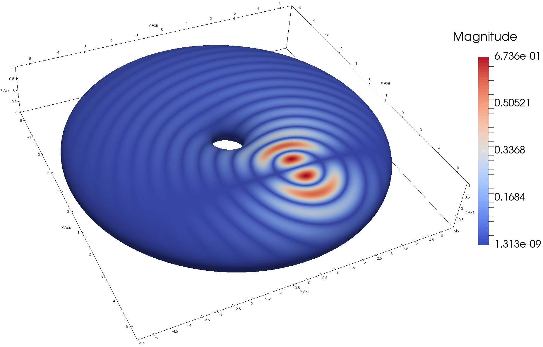
(a) Test geometry and exterior data with $\epsilon_{0}=39.48$ and $\lambda_{0}=1.0$.

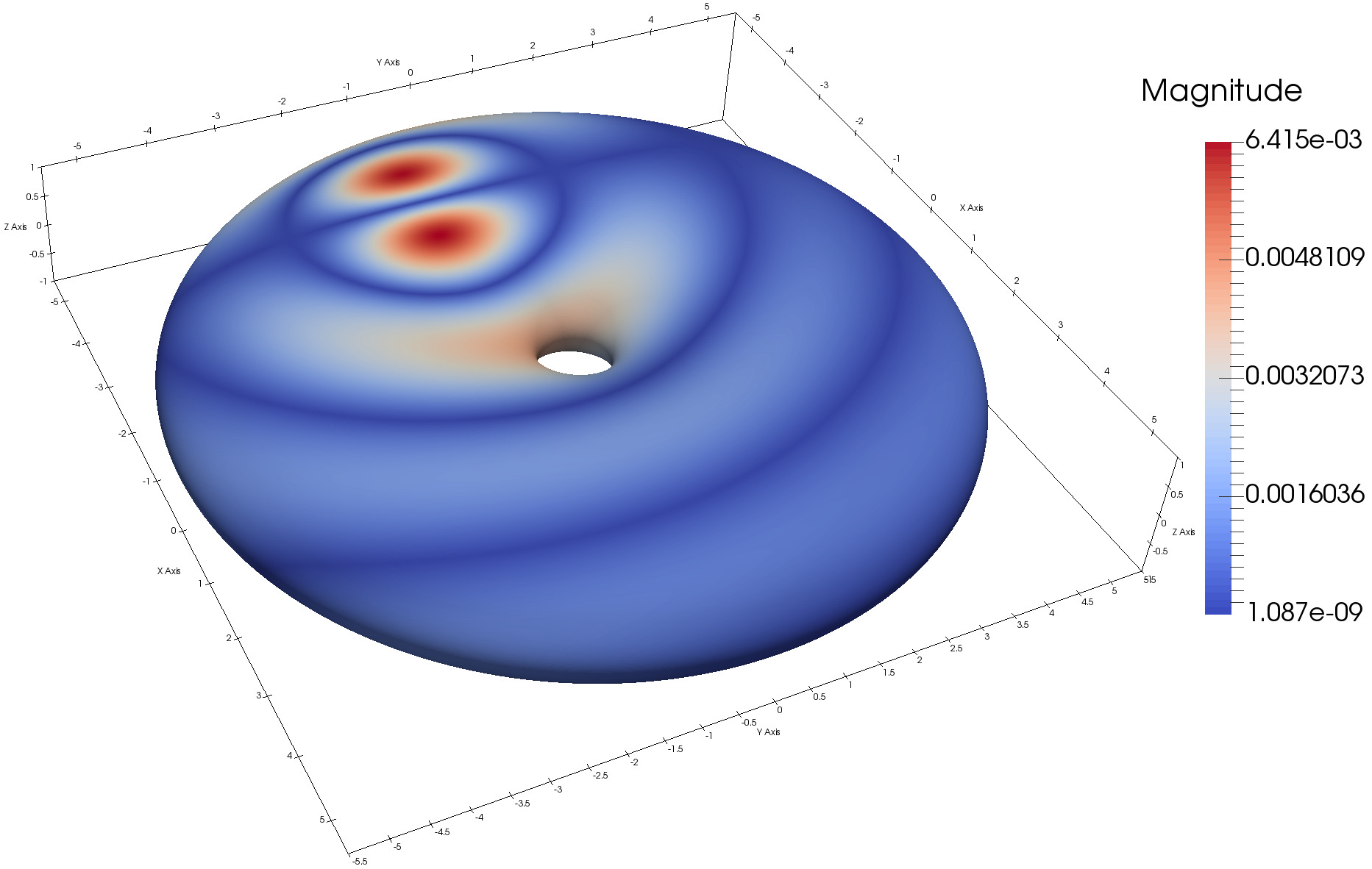
(b) Test geometry and interior data with $\epsilon_{1}=2.47$ and $\lambda_{1}=4.0$.

Figure 4: The geometry for dielectric convergence tests, a 2.5-1 torus centered at the origin. Shown is $|\operatorname{Re}\vectorsym{H}^{\textnormal{in}}|$ along the surface of the scatterer for both the interior data and exterior data. In each case, $\omega=1.0$ and $\mu=1.0$.

Table 2: Convergence results of the solver for scattering from a dielectric region. The exterior test field was generated from a current loop located at $(2.83,1.00,0.10)$ with radius $0.20$ and the interior test field was generated from a current loop located at $(-2.83,-1.00,2.55)$ with radius $0.20$. The integral equation was discretized using 8th-order hybrid Gauss-Trapezoidal quadrature rules [2]. The geometry and data are shown in Figure 4.

$N$	$L$	$NL$	$\operatorname{Res}\Gamma$	$t$	Err($\vectorsym{E}_{0}$)	Err($\vectorsym{H}_{0}$)	Err($\vectorsym{E}_{1}$)	Err($\vectorsym{H}_{1}$)
65	64	4,160	6.2E-04	0.9	7.0E-02	2.2E-02	1.4E-04	5.3E-05
129	128	16,512	1.1E-06	8.3	5.4E-06	5.2E-06	3.0E-07	1.3E-07
257	256	65,792	5.7E-12	85.7	3.6E-09	3.6E-09	2.4E-10	1.5E-09
513	512	262,656	4.1E-15	768.5	1.3E-11	1.4E-11	9.4E-12	3.5E-12

5.2 Varying the order of accuracy of the quadrature rule

We now investigate the effect of the order of accuracy of the quadrature rule on the achieved precision, while also considering some more complicated geometries. We will use the scatterers depicted in Figure 5, whose surfaces are given by

$$\left(\frac{r-r_{0}}{a}\right)^{p}+\left(\frac{z-z_{0}}{b}\right)^{p}=1.$$ (5.7)

The generating curve (i.e. a slice of the above surface for fixed $\theta$) is a super-ellipse in the $\theta z$-plane. The parameter $p$ controls the curvature at the corners, and $a$ and $b$ control the aspect ratio. Geometries such as this are notoriously hard to resolve using equispaced sampling schemes. This generating curve can be parameterized with respect to central angle relative to $(r_{0},0,z_{0})$ as:

$$\vectorsym{\gamma}(t)=\left(r_{0}+\frac{\cos t}{R(t)}\right)\vectorsym{{r}}+\left(z_{0}+\frac{\sin t}{R(t)}\right)\vectorsym{{k}},$$ (5.8)

where

$$R(t)=\left(\left(\frac{\cos t}{a}\right)^{p}+\left(\frac{\sin t}{b}\right)^{p}\right)^{1/p}$$ (5.9)

is the distance from the point $(r_{0},0,z_{0})$ to the boundary (in some $\theta$-slice). This is not an arclength parameterization. In the following calculations, we have set $p=6$, $(r_{0},0,z_{0})=(0.5,0,0)$, $a=0.25$, and the curve has been discretized (i.e. resampled) in arclength. The height parameter $b$ is varied between experiments and given in the captions.

The column labelled $\lambda$ denotes the wavelength, $\lambda=k/2\pi$. As before, the columns labelled $N$ and $L$ denote the number discretization points along the generating curve, in the azimuthal direction, respectively. The columns labelled $N/\lambda$, $L/\lambda$, and $D/\lambda$ denote the number of discretization points per wavelength along the generating curve, the number of discretization points per wavelength along the maximum circumference of the object in the azimuthal direction, and the diameter of the smallest sphere enclosing the object in wavelengths, respectively. The column labelled $q$ denotes the order of accuracy of the quadrature used [2] and $t$ indicates the solution time in seconds.

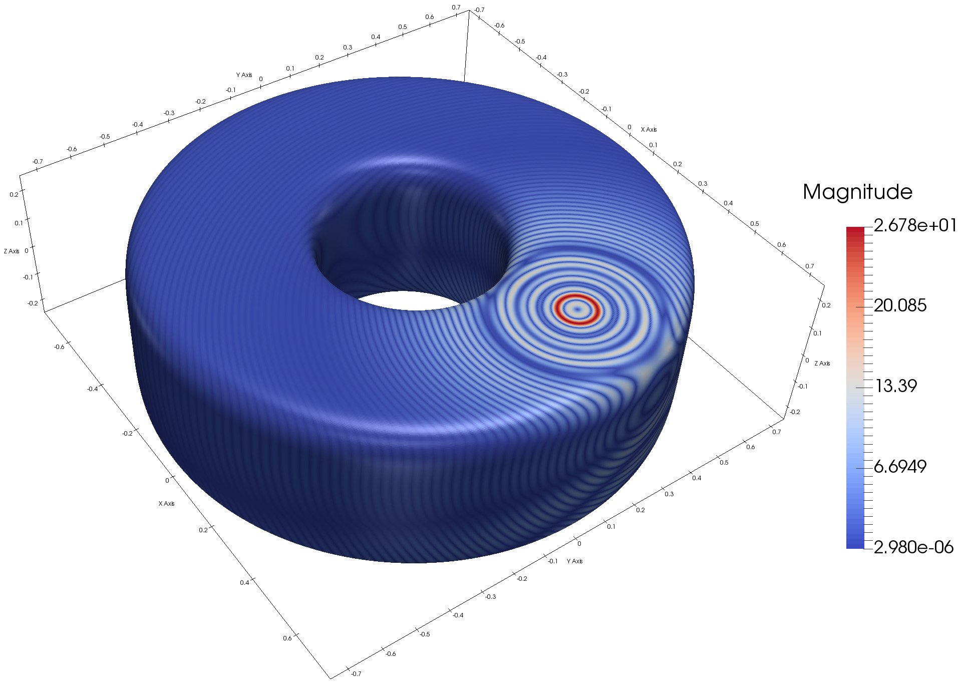
(a) Super-ellipse test geometry (a thick washer) and data $|\operatorname{Re}\vectorsym{E}^{\textnormal{in}}|$ with $b=0.25$ and $\lambda=1/32$.

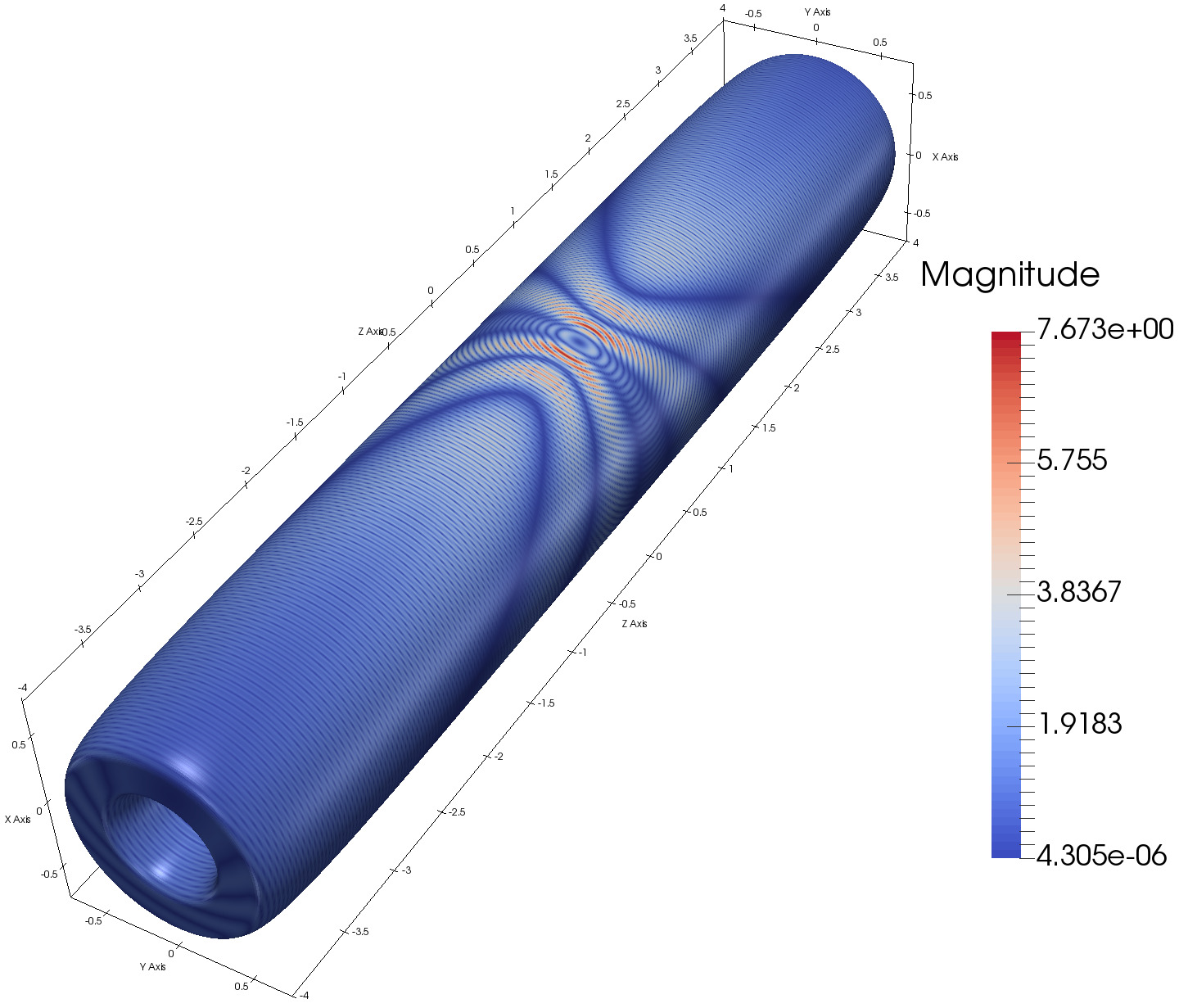
(b) Super-ellipse test geometry (a truncated pipe) and data $|\operatorname{Re}\vectorsym{E}^{\textnormal{in}}|$ with $b=4.0$ and $\lambda=0.06$.

Figure 5: The test geometries for demonstrating convergence as a function of order of the discretization.

We see in Table 3(a) similar accuracies in the solver at large wavelengths, independent of the quadrature order. However, as the wavelength is decreased and the discretization is refined (in order to maintain a constant number of points per wavelength), the 2nd order scheme ceases to converge past a few digits. This is a well-known phenomenon encountered in high frequency wave propagation problems: in order to maintain precision, the order of accuracy of the discretization must be increased as the wavelength decreases (assuming, of course, that the number of discretization points per wavelength is held constant).

Results for a similar test on an elongated super-ellipse are contained in Table 3(b). At higher frequencies, this pipe-like geometry is particularly difficult to handle, as the interior is many cubic wavelengths in size and is a nearly resonant cavity. This example illustrates the importance of discretizing such problems using high-order methods. Table 3(b) shows accuracy results for various order quadrature rules at a fixed discretization size for a relatively small wavelength. With no extra computation time, many more digits of accuracy can be obtained using a high-order discretization than a low-order one. In both examples the error in the computed solution was determined at 50 points on a sphere of radius 8 centered at the origin.

Table 3: Accuracy results of the solver for PEC scattering from the super-ellipse geometry at relatively high frequencies. The exterior test field was generated from a current loop located at $(0.47,0.17,0.10)$ with radius $0.1$. The integral equation was discretized using varying orders of hybrid Gauss-Trapezoidal quadrature rules [2]. The geometries and data are shown in Figure 5.

(a) Convergence for super-ellipse 1 in Figure 5(a), maintaining a constant number of points per wavelength along the generating curve ($N/\lambda$) and along the maximum circumference of the object in the azimuthal direction ($L/\lambda$).

$\lambda$	$N$	$N/\lambda$	$L$	$L/\lambda$	$NL$	$D/\lambda$	$\operatorname{Res}\Gamma$	$q$	$t$	Err($\vectorsym{E}$)	Err($\vectorsym{H}$)
1/2	41	11.2	100	10.6	4,100	3.0	1.2E-02	2	0.4	4.7E-03	4.8E-03
1/4	81	11.1	190	10.0	15,390	6.1	3.5E-04	2	0.6	1.4E-03	1.4E-03
1/8	151	10.3	380	10.0	57,380	12.2	1.2E-06	2	2.1	5.9E-04	5.9E-04
1/16	301	10.3	760	10.0	228,760	24.5	8.4E-12	2	10.0	4.3E-04	4.3E-04
1/32	591	10.0	1510	10.0	892,410	49.0	6.8E-15	2	68.4	4.5E-04	4.5E-04
1/2	41	11.2	100	10.6	4,100	3.0	1.2E-02	4	0.2	2.4E-03	2.6E-03
1/4	81	11.1	190	10.0	15,390	6.1	3.5E-04	4	0.6	2.3E-04	2.3E-04
1/8	151	10.3	380	10.0	57,380	12.2	1.2E-06	4	2.0	3.8E-05	3.8E-05
1/16	301	10.3	760	10.0	228,760	24.5	8.4E-12	4	10.0	1.0E-05	1.0E-05
1/32	591	10.0	1510	10.0	892,410	49.0	6.8E-15	4	67.7	1.0E-07	1.0E-07
1/2	41	11.2	100	0.6	4,100	3.0	1.2E-02	8	0.2	1.9E-03	2.1E-03
1/4	81	11.1	190	10.0	15,390	6.1	3.5E-04	8	0.6	1.9E-05	2.0E-05
1/8	151	10.3	380	10.0	57,380	12.2	1.2E-06	8	1.9	9.1E-07	9.1E-07
1/16	301	10.3	760	10.0	228,760	24.5	8.4E-12	8	10.2	4.6E-08	4.6E-08
1/32	591	10.0	1510	10.0	892,410	49.0	6.8E-15	8	67.8	3.0E-08	3.0E-08
1/2	41	11.2	100	10.6	4,100	3.0	1.2E-02	16	0.2	1.9E-03	2.0E-03
1/4	81	11.1	190	10.0	15,390	6.1	3.5E-04	16	0.7	6.2E-06	7.1E-06
1/8	151	10.3	380	10.0	57,380	12.2	1.2E-06	16	2.2	1.6E-08	1.6E-08
1/16	301	10.3	760	10.0	228,760	24.5	8.4E-12	16	10.5	4.5E-10	4.5E-10
1/32	591	10.0	1510	10.0	892,410	49.0	6.8E-15	16	68.5	3.8E-10	3.8E-10

(b) Accuracy obtained for varying quadrature orders $q$ in the discretization of the elongated super-ellipse (truncated pipe) shown given in Figure 5(b) with $\lambda=0.06$. The pipe is approximately 135$\lambda$ long, making the scattering problem rather ill-conditioned.

$\lambda$	$N$	$N/\lambda$	$L$	$L/\lambda$	$NL$	$D/\lambda$	$\operatorname{Res}\Gamma$	$q$	$t$	Err($\vectorsym{E}$)	Err($\vectorsym{H}$)
0.06	1381	5.0	395	5.0	545,495	134.7	3.2E-07	2	483.5	1.3E-02	1.3E-02
0.06	1381	5.0	395	5.0	545,495	134.7	3.2E-07	4	504.2	1.2E-03	1.2E-03
0.06	1381	5.0	395	5.0	545,495	134.7	3.2E-07	8	491.5	1.9E-04	1.9E-04
0.06	1381	5.0	395	5.0	545,495	134.7	3.2E-07	16	486.6	1.1E-06	1.1E-06

5.3 Computation of radar cross-section

With the previous high-order convergence results in mind, the canonical application of integral equation-based solvers for electromagnetic scattering phenomena is the computation of the radar cross-section (RCS) of an object. Essentially, the radar cross section characterizes the far-field scattering response of an object to an incoming electromagnetic plane-wave and is critical in inverse scattering and object recognition applications.

An incoming electromagnetic plane-wave propagating in the direction $\vectorsym{u}$ with polarization $\vectorsym{p}$ is given by

$$\vectorsym{E}^{\textnormal{in}}(\vectorsym{x}) =\vectorsym{p}\,e^{ik{\vectorsym{u}}\cdot\vectorsym{x}},$$ (5.10)

$$\vectorsym{H}^{\textnormal{in}}(\vectorsym{x}) =\vectorsym{u}\times\vectorsym{p}\,e^{ik\vectorsym{u}\cdot\vectorsym{x}},$$

where it is assumed that $\vectorsym{u}$ and $\vectorsym{p}$ are unit vectors. In order for Maxwell’s equations to be satisfied, we must have $\vectorsym{u}\cdot\vectorsym{p}=0$. The monostatic RCS (MRCS) of an object $\Omega$ degscribes the backscatter of an object in the direction of propagation opposite that of the incoming plane wave. For a body of revolution, it is standard to compute only the $\varphi$-dependence (polar angle) of the MRCS, since for fixed $\pm z$-polarizations the $\theta$-dependence is constant (due to rotational symmetry). Letting $(\rho,\varphi,\theta)$ denote the spherical coordinates with $\theta$ the azimuthal angle, if we set the direction of propagation of the incoming plane-wave to be $\vectorsym{u}=-\sin\varphi\,\vectorsym{{i}}-\cos\varphi\,\vectorsym{{k}}$, then a horizontally-polarized plane wave is given by:

$$\vectorsym{E}^{\textnormal{in}}(\vectorsym{x}) =\vectorsym{{j}}\,e^{-ik(x\sin\varphi+z\cos\varphi)},$$ (5.11)

$$\vectorsym{H}^{\textnormal{in}}(\vectorsym{x}) =(\cos\varphi\,\vectorsym{{i}}-\sin\varphi\,\vectorsym{{k}})\,e^{-ik(x\sin\varphi+z\cos\varphi)},$$

where as before, $(\vectorsym{{i}},\vectorsym{{j}},\vectorsym{{k}})$ are the unit vectors in the Cartesian coordinate system. As a function of $\varphi$, the MRCS in this setup is then approximately [28, 29]:

$$\text{MRCS}(\varphi) \approx 4\pi R^{2}\,\frac{|\vectorsym{E}(\vectorsym{x}_{R}(\varphi))|^{2}}{|\vectorsym{E}^{\textnormal{in}}(\vectorsym{x}_{R}(\varphi))|^{2}}$$ (5.12)

$$=4\pi R^{2}\,|\vectorsym{E}(\vectorsym{x}_{R}(\varphi))|^{2}$$

since $|\vectorsym{E}^{\textnormal{in}}|=1$, where $R$ is some fixed distance (set to be 10 in the subsequent experiments) from the center of the object (assumed to be the origin of the coordinate system in this example) and $\vectorsym{x}_{R}(\varphi)=R\sin\varphi\,\vectorsym{{i}}+R\cos\varphi\,\vectorsym{{k}}$. Take care to note that the observation point $\vectorsym{x}_{R}$ lies in the direction opposite the direction of propagation of the incoming plane wave. Shown in Figure 6(a) is a plot of the real-part of the induced generalized Deybe source  $\rho$ along $\Omega$, $\operatorname{Re}\rho$ (see equation (2.16)), and the real-part of the $x$-component of the total field, $\operatorname{Re}E^{\text{tot}}_{x}$, along the enclosing walls. The incoming plane wave was assumed to be propagating in the direction $(-1/\sqrt{2},0,-1/\sqrt{2})$ with polarization $(0,1,0)$. In Figure 6(b) we plot the MCRS as a function of the polar angle of incidence, $\varphi\in[0,\pi]$, for various refinements of the discretization. Following convention, we report the MRCS on a decibel scale: $10\,\log_{10}\text{MRCS}$. In these examples, we set $\lambda=0.5$ so that the pipe is approximately 16 wavelengths long. The pipe was discretized with $N=129$, $N=513$, and $N=1025$ points along the generating curve, and $L$ was set so as to maintain the same number of points per wavelength along the azimuthal direction.

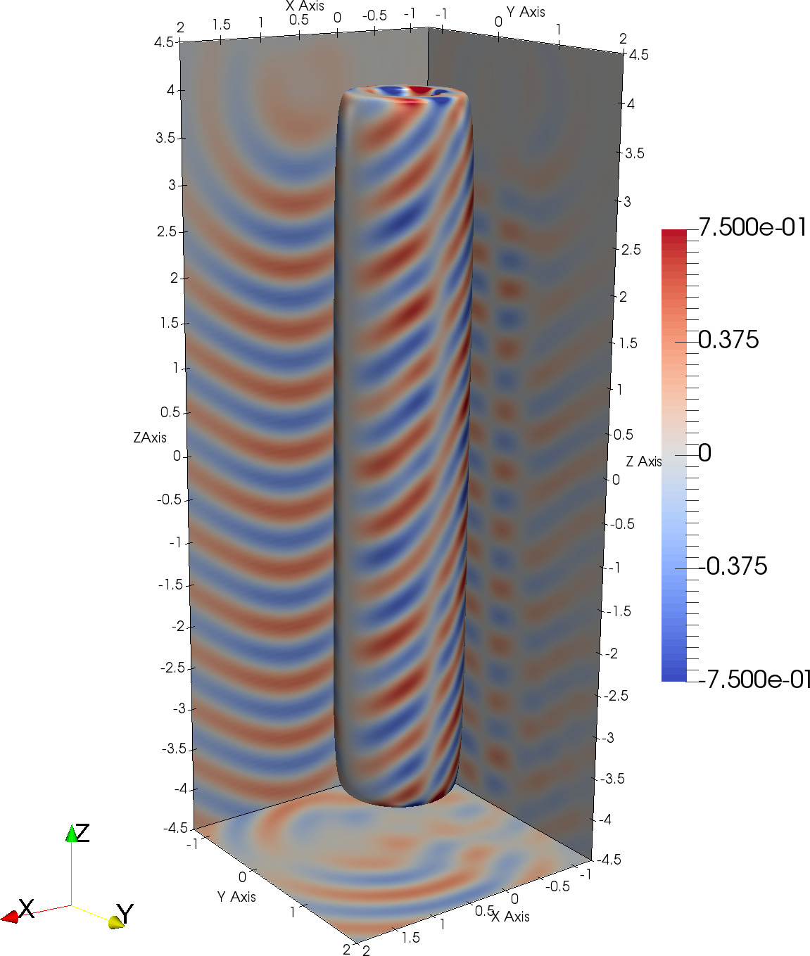
(a) The induced generalized Debye source $\rho$ and the total field on an enclosing box.

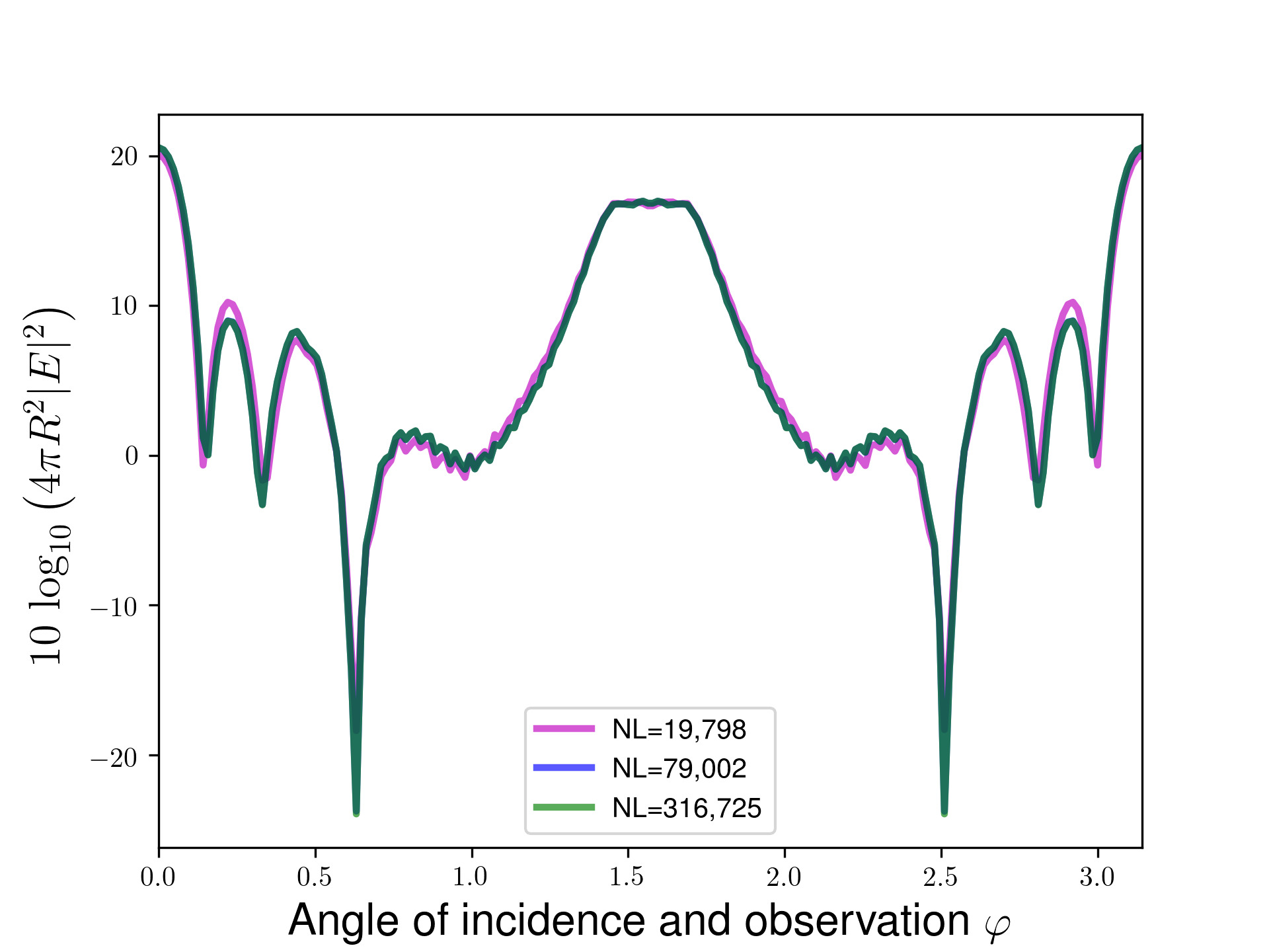
(b) The monostatic radar cross section of the pipe geometry for a horizontally polarized incoming plane wave.

Figure 6: Plots of the scattered field from an incident plane wave and the monostatic radar cross section for the pipe geometry.

These experiments correspond to true scattering problems, for which the exact solution is not known. Since the data are very regular and smooth (in fact smoother than the data in the previous examples) the accuracy can be estimated from Table 3(b). The accuracy can also be estimated by a self-convergence study, as shown in the column labeled Err(MRCS) in Table 4. This error is the relative $\ell^{2}$ error in the quantity $10\,\log_{10}MRCS$. We see that the errors are approximately commensurate with the geometry resolution, and comparable to the results in the high-frequency case in the previous subsection. Furthermore, since we are using a direct solver, the system can be set up and factored once, so that each subsequent MRCS calculation merely requires the application of the inverse to a new right hand side, greatly accelerating the calculation.

Table 4: Data for the monostatic radar cross section plot in Figure 6(b). The relative $\ell^{2}$ error is computed via a self-convergence test at 200 equispaced points in the polar angle direction at a distance of $R=10$.

$\lambda$	$N$	$N/\lambda$	$L$	$L/\lambda$	$NL$	$D/\lambda$	$\operatorname{Res}\Gamma$	Err(MRCS)
0.5	257	7.8	77	8.2	19,789	8.1	1.2E-02	1.1E-01
0.5	513	15.5	154	16.3	79,002	8.1	1.2E-03	2.6E-03
0.5	1025	31.0	309	32.8	316,725	8.1	1.4E-05

6 Conclusions

We have presented a direct solver based on the generalized Debye integral equation framework for full electromagnetic scattering from perfect electric conductors or dielectric bodies which are rotationally symmetric. Unlike most widely used formulations, our approach is invertible for all passive materials at any frequency, and immune from both dense-mesh breakdown and topological low frequency breakdown.

The scheme makes use of separation of variables in the azimuthal direction, leading to a collection of smaller, uncoupled integral equations on curves. The implementation described in this work relies on a trapezoidal-based Nyström discretization, restricting its applicability to geometries which are reasonably well-discretized using equispaced nodes in some parameterization. Alternative discretizations and quadrature rules are required for scatterers whose generating curves contain corner singularities, but the overall approach would remain the same. For large scale problems, the bulk of the computation is spent in BLAS3 routines, assembling the system matrix (due to the composition of several integral operators in the representation). These matrix assembly steps are highly parallelizable.

We are presently working on implementing solvers for the generalized Debye integral equations on more general (closed) surfaces in three dimensions.

References

- Ahrens et al. [2005] J. Ahrens, B. Geveci, and C. Law. Paraview: An end-user tool for large data visualization. In C. D. Hansen and C. R. Johnson, editors, The Visualization Handbook. Elsevier, 2005.
- Alpert [1999] B. Alpert. Hybrid Gauss-trapezoidal quadrature rules. SIAM J. Sci. Comput., 20(5):1551–1584, 1999.
- Atkinson [1997] K. E. Atkinson. The Numerical Solution of Integral Equations of the Second Kind. Cambridge University Press, New York, NY, 1997.
- Barnett and Betcke [2008] A. H. Barnett and T. Betcke. Stability and convergence of the method of fundamental solutions for Helmholtz problems on analytic domains. Journal of Computational Physics, 227(14):7003–7026, 2008.
- Bremer and Gimbutas [2013] J. Bremer and Z. Gimbutas. On the numerical evaluation of singular integrals of scattering theory. J. Comput. Phys., 251:327–343, 2013.
- Briggs and Henson [1995] W. L. Briggs and V. E. Henson. The DFT: An Owner’s Manual for the Discrete Fourier Transform. SIAM, Philadelphia, PA, 1995.
- Chew et al. [2001] W. C. Chew, E. Michielssen, J. M. Song, and J. M. Jin. Fast and Efficient Algorithms in Computational Electromagnetics. Artech House, Inc., Norwood, MA, 2001.
- Cohl and Tohline [1999] H. S. Cohl and J. E. Tohline. A compact cylindrical Green’s function expansion for the solution of potential problems. Astrophys. J., 527(1):86–101, 1999.
- Colton and Kress [1983] D. Colton and R. Kress. Integral Equation Methods in Scattering Theory. John Wiley & Sons, Inc., 1983.
- Contopanagos et al. [2002] H. Contopanagos, B. Dembart, M. Epton, J. J. Ottusch, V. Rokhlin, J. L. Visher, and S. M. Wandzura. Well-conditioned boundary integral equations for three-dimensional electromagnetic scattering. IEEE Trans. Antennas Propag., 50(12):1824–1830, 2002.
- Conway and Cohl [2010] J. T. Conway and H. S. Cohl. Exact Fourier expansion in cylindrical coordinates for the three-dimensional Helmholtz Green function. Z. Angew. Math. Phys., 61:425–442, 2010.
- Cools et al. [2009] K. Cools, F. P. Andriulli, F. Olyslager, and E. Michielssen. Nullspaces of MFIE and Calderon Preconditioned EFIE Operators Applied to Toroidal Surfaces. IEEE Trans. Antennas Propag., 57(10):3205–3215, 2009.
- Epstein and Greengard [2010] C. L. Epstein and L. Greengard. Debye sources and the numerical solution of the time harmonic Maxwell equations. Commun. Pure Appl. Math., 63(4):413–463, 2010.
- Epstein et al. [2013a] C. L. Epstein, Z. Gimbutas, L. Greengard, A. Klöckner, and M. O’Neil. A consistency condition for the vector potential in multiply-connected domains. IEEE Trans. Magn., 49(3):1072–1076, 2013a.
- Epstein et al. [2013b] C. L. Epstein, L. Greengard, and M. O’Neil. Debye sources and the numerical solution of the time harmonic Maxwell equations II. Commun. Pure. Appl. Math., 66(5):753–789, 2013b.
- Epstein et al. [2015] C. L. Epstein, L. Greengard, and M. O’Neil. Debye sources, Beltrami fields, and a complex structure on Maxwell fields. Commun. Pure. Appl. Math., 68:2237–2280, 2015.
- Fairweather and Karageorghis [1998] G. Fairweather and A. Karageorghis. The method of fundamental solutions for elliptic boundary value problems. Advances in Computational Mathematics, 9(1-2):69, 1998.
- Frankel [2011] T. Frankel. The Geometry of Physics. Cambridge University Press, New York, NY, 2011.
- Frittelli and Sgura [2016] M. Frittelli and I. Sgura. Virtual element method for the Laplace-Beltrami equation on surfaces. 2016. arXiv:1612.02369 [math.NA].
- Gedney and Mittra [1990] S. D. Gedney and R. Mittra. The use of the FFT for the efficient solution of the problem of electromagnetic scattering by a body of revolution. IEEE Trans. Antennas Propag., 38(3):313–322, 1990.
- Gil et al. [2007] A. Gil, J. Segura, and N. M. Temme. Numerical Methods for Special Functions. SIAM, Philadelphia, PA, 2007.
- Gimbutas and Greengard [2013] Z. Gimbutas and L. Greengard. Fast multi-particle scattering: A hybrid solver for the Maxwell equations in microstructured materials. J. Comput. Phys., 232(1):22–32, 2013.
- Gustafsson [2010] M. Gustafsson. Accurate and efficient evaluation of modal Green’s functions. J. Electromagnet. Wave., 24(10):1291–1301, 2010.
- Hao et al. [2014] S. Hao, A. H. Barnett, P.-G. Martinsson, and P. Young. High-order accurate Nyström discretization of integral equations with weakly singular kernels on smooth curves in the plane. Adv. Comput. Math., 40:245–272, 2014.
- Helsing and Karlsson [2014] J. Helsing and A. Karlsson. An explicit kernel-split panel-based Nyström scheme for integral equations on axially symmetric surfaces. J. Comput. Phys., 272:686–703, 2014.
- Helsing and Karlsson [2015] J. Helsing and A. Karlsson. Determination of normalized magnetic eigenfields in microwave cavities. IEEE Transactions on Microwave Theory and Techniques, 63(5):1457–1467, 2015.
- Imbert-Gerard and Greengard [2017] L.-M. Imbert-Gerard and L. Greengard. Pseudo-spectral methods for the Laplace-Beltrami equation and the Hodge decomposition on surfaces of genus one. Numer. Methods Partial. Differ. Equ., 33(3):941–955, 2017.
- Jackson [1999] J. D. Jackson. Classical Electrodynamics. Wiley, New York, NY, 3rd edition, 1999.
- Jin [2010] J.-M. Jin. Theory and Computation of Electromagnetic Fields. IEEE Press, Piscataway, NJ, 2010.
- Kapur and Long [1998] S. Kapur and D. E. Long. IES3: Efficient electrostatic and electromagnetic simulation. Comput. Sci. & Engrg., pages 60–67, 1998.
- Kirsch and Monk [1995] A. Kirsch and P. Monk. A finite element/spectral method for approximating the time-harmonic Maxwell system in . SIAM J. Appl. Math., 55(5):1324–1344, 1995.
- Kucharski [2000] A. A. Kucharski. A method of moments solution for electromagnetic scattering by inhomogeneous dielectric bodies of revolution. IEEE Trans. Antennas Propag., 48(8):1202–1210, 2000.
- Liu and Barnett [2016] Y. Liu and A. H. Barnett. Efficient numerical solution of acoustic scattering from doubly-periodic arrays of axisymmetric objects. J. Comput. Phys., 324:226–245, 2016.
- Mautz and Harrington [1979] J. R. Mautz and R. F. Harrington. Electromagnetic scattering from a homogeneous material body of revolution. Archiv Elektronik und Uebertragungstechnik, 33:71–80, 1979.
- Monk [1992] P. Monk. A finite element method for approximating the time-harmonic Maxwell equations. Numerische Mathematik, 63(1):243–261, 1992.
- Müller [1969] C. Müller. Foundations of the Mathematical Theory of Electromagnetic Waves. Springer-Verlag, Berlin, Heidelberg, 1969.
- Nedelec [2001] J.-C. Nedelec. Acoustic and Electromagnetic Equations. Springer, New York, NY, 2001.
- Olver et al. [2010] F. W. Olver, D. W. Lozier, R. F. Boisvert, and C. W. Clark. NIST Handbook of Mathematical Functions. Cambridge University Press, New York, NY, USA, 1st edition, 2010. ISBN 0521140633, 9780521140638.
- O’Neil [2018] M. O’Neil. Second-kind integral equations for the Laplace-Beltrami problem on surfaces in three dimensions. Adv. Comput. Math., 2018. To appear.
- O’Neil and Cerfon [2018] M. O’Neil and A. J. Cerfon. An integral equation-based numerical solver for Taylor states in toroidal geometries. J. Comput. Phys., 359:263–282, 2018.
- Papas [1988] C. H. Papas. Theory of Electromagnetic Wave Propagation. Dover, New York, NY, 1988.
- Sidi and Israeli [1988] A. Sidi and M. Israeli. Quadrature methods for periodic singular and weakly singular Fredholm integral equations. J. Sci. Comput., 3(2):201–231, 1988.
- Sifuentes et al. [2015] J. Sifuentes, Z. Gimbutas, and L. Greengard. Randomized methods for rank-deficient linear systems. Elec. Trans. Num. Anal., 44:177–188, 2015.
- Taskinen and Yla-Oijala [2006] M. Taskinen and P. Yla-Oijala. Current and charge integral equation formulation. IEEE Trans. Antennas Propag., 54(1):58–67, 2006.
- Trefethen [2000] L. N. Trefethen. Spectral methods in MATLAB. SIAM, Philadelphia, PA, 2000.
- Vico et al. [2013] F. Vico, Z. Gimbutas, L. Greengard, and M. Ferrando-Bataller. Overcoming low-frequency breakdown of the magnetic field integral equation. IEEE Trans. Antennas Propag., 61(3):1285–1290, 2013.
- Vico et al. [2016] F. Vico, M. Ferrando, L. Greengard, and Z. Gimbutas. The decoupled potential integral equation for time-harmonic electromagnetic scattering. Comm. Pure Appl. Math., 69:771–812, 2016.
- Viola [1995] M. S. Viola. A new electric field integral equation for heterogeneous dielectric bodies of revolution. IEEE Transactions on Microwave Theory and Techniques, 43:230–233, 1995.
- Wright et al. [2015] G. B. Wright, M. Javed, H. Montanelli, and L. N. Trefethen. Extension of Chebfun to periodic functions. SIAM J. Sci. Comput., 37:C554–C573, 2015.
- Yee [1966] K. Yee. Numerical solution of initial boundary value problems involving Maxwell’s equations in isotropic media. IEEE Trans. Antennas Propag., 14:302–307, 1966.
- Young et al. [2012] P. Young, S. Hao, and P.-G. Martinsson. A high-order Nyström discretization scheme for boundary integral equations defined on rotationally symmetric surfaces. J. Comput. Phys., 231(11):4142–4159, 2012.
- Youssef [1989] N. N. Youssef. Radar cross section of complex targets. Proc. IEEE, 77:722–734, 1989.