Pricing for Online Resource Allocation: Intervals and Paths

Abstract

We present pricing mechanisms for several online resource allocation problems which obtain tight or nearly tight approximations to social welfare. In our settings, buyers arrive online and purchase bundles of items; buyers’ values for the bundles are drawn from known distributions. This problem is closely related to the so-called prophet-inequality of Krengel and Sucheston [22] and its extensions in recent literature. Motivated by applications to cloud economics, we consider two kinds of buyer preferences. In the first, items correspond to different units of time at which a resource is available; the items are arranged in a total order and buyers desire intervals of items. The second corresponds to bandwidth allocation over a tree network; the items are edges in the network and buyers desire paths.

Because buyers’ preferences have complementarities in the settings we consider, recent constant-factor approximations via item prices do not apply, and indeed strong negative results are known. We develop static, anonymous bundle pricing mechanisms.

For the interval preferences setting, we show that static, anonymous bundle pricings achieve a sublogarithmic competitive ratio, which is optimal (within constant factors) over the class of all online allocation algorithms, truthful or not. For the path preferences setting, we obtain a nearly-tight logarithmic competitive ratio. Both of these results exhibit an exponential improvement over item pricings for these settings. Our results extend to settings where the seller has multiple copies of each item, with the competitive ratio decreasing linearly with supply. Such a gradual tradeoff between supply and the competitive ratio for welfare was previously known only for the single item prophet inequality.

1 Introduction

Consider an online resource allocation setting in which a seller offers multiple items for sale and buyers with preferences over bundles of items arrive over time. We desire an incentive-compatible mechanism for allocating items to buyers that maximizes social welfare—the total value obtained by all the buyers from the allocation. In the offline setting, this is easily achieved by the VCG mechanism. In the online context, however, we would like the mechanism to allocate items and charge payments as buyers arrive, without waiting for future arrivals. What would such a mechanism look like, and can it obtain close to the optimal social welfare?

We consider two settings for online resource allocation motivated by applications in cloud economics. In the interval preferences setting, a cloud provider has multiple copies of a single resource available to allocate over time. Customers have jobs that require renting the resource for some amount of time. If we think of each time unit as a different item, customers desire intervals of items. Different intervals, corresponding to scheduling a job at different times or renting the resource for different lengths of time, may bring different values to the customer. This model closely follows the framework described in [4]. Our second setting, the path preferences setting, models bandwidth allocation over a communication network. Each customer is a source-sink pair in the network that wishes to communicate, and assigns values to paths in the network between the source and the sink. The items are the edges in the network. We focus on the special case where the network is a tree. See [19] for further motivation behind this setting.

It is easy to observe that because of the online nature of the problem no algorithm for online resource allocation, truthful or otherwise, can obtain optimal social welfare: the competitive ratio is at least $2$ even when there is only a single item for sale and the seller knows both the order of arrival of buyers as well as their value distributions. In a remarkable result, Feldman et al. [15] showed that this gap of 2 is the worst possible over a large class of buyer preferences: a particularly simple and natural incentive-compatible mechanism, namely posted item pricing, achieves a $2$-approximation to the optimal social welfare in those settings.

Posted pricing is perhaps the most ubiquitous real-world mechanism for allocating goods to consumers. Supermarkets are a familiar example: the store determines prices for items, which may be sold individually or packaged into bundles. Customers arrive in arbitrary order and purchase the items they most desire at the advertised prices, unless they’re sold out. Many other domains have a similar sequential posted pricing format, from airfares to online retail to concert tickets. Feldman et al.’s results apply to settings where buyers’ values over bundles of items are fractionally subadditive, a.k.a. XOS. In these settings, the seller determines a price for each item based on his knowledge of the buyers’ value distributions. These prices are anonymous and static, meaning that the same prices are offered to each customer and remain unchanged until supply runs out.

However, the settings we consider exhibit complementarity in buyers’ values: buyers may require certain minimal bundles of items to satisfy their requirements; anything less brings them zero value. For these settings, Feldman et al. [15] show that anonymous item pricings cannot achieve a competitive ratio better than linear in the degree of complementarity (that is, the size of the minimal desired bundle of items). See Footnote 3 for an example. Is a better competitive ratio possible? Can it be achieved through a truthful mechanism as simple as static, anonymous item pricings?

We show that near-optimal competitive ratios can be achieved for the interval and path preferences settings via a static, anonymous bundle pricing mechanism.

Our mechanism is a posted bundle pricing: the seller partitions items into bundles, and prices each bundle based on his knowledge of the distribution of buyers’ preferences. Customers arrive in arbitrary order and purchase the bundles they most desire at the advertised prices, unless they’re sold out. As in Feldman et al.’s work, our bundle pricings are static and anonymous.

We now elaborate on our results and techniques.

1.1 Our results

Recall that in the interval preferences setting, items are arranged in a total order and buyers desire intervals of items. We assume that each buyer’s value function is drawn independently from some arbitrary but known distribution over possible value vectors. The seller’s computational problem is essentially a stochastic online interval packing. Let $L$ denote the length of the longest interval that may be desired by some buyer. Feldman et al. [15] show that no item pricing can achieve a $o(L)$ competitive ratio in this setting. Im and Wang [18] previously showed that in fact no online algorithm can achieve a competitive ratio of $o\left(\frac{\log L}{\log\log L}\right)$. Our first main result matches this lower bound to within constant factors.

Theorem 1.1.

For the interval preferences setting, there exists a static, anonymous bundle pricing with competitive ratio $O\left(\frac{\log L}{\log\log L}\right)$ for social welfare.

The interval preferences setting was studied recently by Chawla et al. [11], who also designed a static item pricing mechanism for the problem. Chawla et al. showed that when the item supply is large, specifically, when the seller has $\tilde{\Omega}(L^{6}/\varepsilon^{3})$ copies of each item for some $\varepsilon>0$, static anonymous item pricings achieve a $1-\varepsilon$ approximation to social welfare. Chawla et al.’s result suggests that there is a tradeoff between item supply and the performance of posted pricings in this setting. Our second main result maps out this tradeoff exactly (to within constant factors) for bundle pricing. We show that the approximation factor decreases inversely with item supply, and is a constant when supply is $\Omega(\log L)$. In other words, to achieve a constant approximation via bundle pricing, we require an exponentially smaller bound on the item supply relative to that required by Chawla et al. for a $1-\varepsilon$ approximation. Furthermore, this tradeoff is tight to within constant factors.

Theorem 1.2.

For the interval preferences setting, if every item has at least $B>0$ copies available, then a static, anonymous bundle pricing achieves a competitive ratio of

$$O\left(\frac{1}{B}\frac{\log L}{\log\log L-\log B}\right)$$

when $B<\log L$, and $O(1)$ otherwise.

Theorem 1.3.

For the interval preferences setting, if every item has at least $B>0$ copies available, no online algorithm can obtain a competitive ratio of $o\left(\frac{1}{B}\frac{\log L}{\log\log L}\right)$ for social welfare.

We then turn to the path preferences setting, which appears to be considerably harder than the special case of interval preferences. In this setting buyers are single-minded in that they desire a particular path, although their value for this path is unknown to the seller. As before let $L$ denote the length of the longest bundle/path that any buyer desires. We first observe that no online algorithm can achieve a subpolynomial in $L$ competitive ratio for this setting (see Theorem 4.3). We therefore explore competitive ratios as functions of $H$, the ratio of the maximum possible value to the minimum possible non-zero value. In terms of $H$, the construction of Im and Wang [18] provides a lower bound of $\Omega(\log H/\log\log H)$ on the competitive ratio of any online algorithm. We nearly match this lower bound:

Theorem 1.4.

For the path preferences setting, there exists a static, anonymous bundle pricing with competitive ratio $O\left(\log H\right)$ for social welfare.

As for the interval preferences setting, we obtain a linear tradeoff between item supply and the performance of bundle pricing for the path preferences setting.

Theorem 1.5.

For the path preferences setting, if every edge has at least $B>0$ copies available, then a static, anonymous bundle pricing achieves a competitive ratio of $O\left(\frac{1}{B}\log H\right)$ for welfare.

Theorems 1.1 and 1.2 for the interval preferences setting are proved in Section 3. Section 4 presents the lower bounds—Theorems 1.3 and 4.3. Our main results for the path preferences setting, Theorem 1.4 and Theorem 1.5, are proved in Section 5. Some of our results extend with the same competitive ratios to settings with non-decreasing marginal production costs instead of a fixed supply; this setting is discussed in Section 6. Any proofs skipped in the main body of the paper can be found in Section 7.

All of our theorems are constructive but require an explicit description of the buyers’ value distributions. The pricings guaranteed above can be constructed in time polynomial in the sum over the buyers of the sizes of the supports of their value distributions.

1.2 Related work and our techniques

Competitive ratios for welfare in online settings are known as prophet inequalities following the work of Krengel and Sucheston [22] and Samuel-Cahn [25] on the special case of allocating a single item. Most arguments for prophet inequalities follow a standard approach, introduced by Kleinberg and Weinberg [21] and further developed by Feldman et al. [15], of setting “balanced” prices or thresholds for each buyer: informally, prices should be low enough that buyers can afford their optimal allocations, and at the same time high enough so that allocating items non-optimally recovers as revenue a good fraction of the optimal welfare that is “blocked” by that allocation. Given such balanced prices, we can then account for the social welfare of the online allocation in two components—the seller’s share of the welfare, namely his revenue, and the buyers’ share of the welfare, namely their utility. On the one hand, the prices of any items/bundles sold by the mechanism contribute to the seller’s revenue. On the other hand, any item/bundle that goes unsold in the online allocation contributes to the buyers’ utility: the buyer who receives it in the optimal allocation forgoes it in the online allocation for another one with even higher utility. The argument asserts that in either case good social welfare is achieved.

When buyers have values with complements and an item pricing is used this argument breaks down. In particular, it may be the case that a bundle allocated by the optimal solution goes unsold because only one of the items in the bundle is sold out. The loss of the buyer’s utility in this case may not be adequately covered by the revenue generated by the sold subset of items. We therefore consider pricing bundles of items.

Recently Duetting et al. [14] developed a framework for obtaining balanced prices via a sort of extension theorem. They showed that if one can define prices achieving a somewhat stronger balance condition in the full-information setting, where the seller knows the buyers’ value functions exactly, then a good approximation through posted prices can be obtained in the Bayesian setting as well. A significant benefit of using this approach is that it suffices to focus on the full-information setting, and the designer need no longer worry about the value distribution.

In the full-information setting, even with arbitrary values over bundles of items, it is easy to construct a static, anonymous bundle pricing that achieves a $2$-approximation for welfare, as demonstrated, for example, by Cohen-Addad et al. [12]. Unfortunately, these prices do not satisfy the strong balance condition of Duetting et al. In fact we do not know of any distribution-independent way of defining bundle prices in the full information setting that satisfy the balance condition of Duetting et al. with approximation factors matching the ones we achieve. Furthermore, while a main goal of our work is to establish a tradeoff between supply and competitive ratio for welfare, the framework of Duetting et al. does not seem to lend itself to such a tradeoff.

The crux of our argument for both of our settings lies in constructing a distribution-dependent partition of items into bundles, and pricing (subsets of) these bundles. For the interval preferences setting we construct a partition for which there exists an allocation of bundles to buyers such that each buyer receives at most one bundle and a good fraction of the social welfare is achieved. Given such a bundling, we are essentially left with a “unit-demand” setting for which a prophet inequality can be constructed using the techniques described above. We call such an allocation a unit allocation. The main technical depth of this result lies in constructing such a bundling.

In fact, it is straightforward to construct a bundling that leads to an $O(\log L)$ competitive ratio: pick a random power of $2$ between $1$ and $L$; partition items into intervals of that length starting with a random offset; and construct an optimal allocation that allocates entire bundles in the constructed partition. However, our improved $O(\log L/\log\log L)$ approximation requires much more care in partitioning items into bundles of many different sizes, and requires the partitioning to be done in a distribution-dependent manner.

As mentioned earlier, the path preferences setting generalizes interval preferences, but appears to be much harder. In particular, we don’t know how to obtain a constant competitive ratio even when all desired paths are of equal length. We show, however, that if all buyers have equal values and all edges have equal capacity, it becomes possible to identify up to two most contentious edges on every path, and the problem behaves like one where every buyer desires only two items. For this special case, it becomes possible to construct a pricing using techniques from [15]. Unfortunately, this argument falls apart when different items have different multiplicity. In order to deal with multiplicities, we present a different kind of partitioning of items into bundles or layers and a constrained allocation that we call a layered allocation, such that each layer behaves like a unit-capacity setting. These ideas altogether lead to an $O(\log H)$ competitive ratio.

As mentioned previously, our approach lends itself to achieving tradeoffs between item supply and competitive ratio. On the one hand, when different items are available to different extents, we need to be careful in constructing a partition into bundles and in some places this complicates our arguments. On the other hand, large supply allows us some flexibility in partitioning the instance into multiple smaller instances, leading to improved competitive ratios. The key to enabling this partitioning is a composability property of our analysis: suppose we have multiple disjoint instances of items and buyers, for each of which in isolation our argument provides a good welfare guarantee; then running these instances together and allowing buyers to purchase bundles from any instance provides at least half the sum of the individual welfares. In the path preferences setting, obtaining this composability crucially requires buyers to be single-minded.

Discussion and open questions.

Two implications of our results seem worthy of further study. First, for the settings we consider as well as those studied previously, posted pricings perform nearly as well as arbitrary online algorithms, truthful or not. Can this be formalized into a meta-theorem that holds for broader contexts? Second, a modest increase in supply brings about significant improvements in competitive ratio for the settings we study. However, once the competitive ratio hits a certain constant factor, our techniques do not provide any further improvement. Can this tradeoff be extended all the way to a $1+\epsilon$ competitive ratio?

Another natural open problem is to extend our guarantees for the path preferences setting to general graphs. This appears challenging. Our arguments rely on a fractional relaxation of the optimal allocation. General graphs exhibit an integrality gap that is polynomial in the size of the graph even when all buyers are single-minded, have the same values (0 or 1 with some probability), and have identical path lengths; this integrality gap is driven by the combinatorial structure exhibited by paths in graphs. Indeed this setting appears to be as hard as the most general setting with no constraints on buyers’ values. It may nevertheless be possible to obtain a non-trivial competitive ratio relative to a different relaxation of the offline optimum.

Other related work.

Sequential pricing mechanisms (SPMs) were first studied for the problem of revenue maximization, where computing the optimal mechanism is a computationally hard problem and no simple characterizations of optimal mechanisms are known. A series of works (e.g., [8, 5, 9, 10, 3, 24, 7, 6]) showed that in settings where buyers have subadditive values, SPMs achieve constant-factor approximations to revenue. In most interesting settings, good approximations to revenue necessarily require non-anonymous pricings. As a result, techniques in this literature are quite different from those for welfare. [16] gives (non-truthful) online algorithms which obtain constant-factor approximations in our settings when supply is unit-capacity, buyers are single-minded, and all values are identical. There is also a long line of work on welfare-maximizing mechanisms with buyers arriving online in the worst case setting where the seller has no prior information about buyers’ values [23, 17, 13, 1, 2, 11]. The worst case setting generally exhibits very different techniques and results relative to the Bayesian setting we study.

2 Model and definitions

We consider a setting with $n$ buyers and a set of items $T$. We index buyers by $i$ and items by $t$ (or $e$ for edges). Buyer $i$’s valuation function is denoted $v_{i}:2^{T}\rightarrow\Re^{+}$, with $v_{i}(\emptyset)=0$. Our setting is Bayesian: $v_{i}$ is drawn from a distribution $F_{i}$ that is independent of other buyers and known to the seller. We emphasize that values may be correlated across bundles, but not across buyers. Let $B_{t}$ denote the number of copies available, a.k.a. supply or capacity, for item $t$. Let $B=\min_{t}B_{t}$. The unit-capacity setting is a special case where $B=1$. An allocation is an assignment of bundles of items to buyers such that no item is allocated more than its number of copies available. Our goal is to maximize the buyers’ total welfare—that is, the sum over values each buyer derives from his allocated bundle.

Jobs.

We now describe assumptions and notational shortcuts for buyers’ value functions that hold without loss of generality and simplify exposition. First, we assume that values are monotone: for all $i$ and $v_{i}$, and all bundles $S\subset S^{\prime}\subseteq T$, $v_{i}(S)\leq v_{i}(S^{\prime})$. Second, we assume that each buyer’s value distribution is a discrete distribution with finite support. In other words, each buyer $i$ can only have finitely many possible valuation functions: with probability ${q_{v_{i}}}$, buyer $i$’s values are given by the known function $v_{i}$.

Third, we think of a buyer $i$ with value function $v_{i}$ as being a collection of “jobs” represented by tuples $(i,v_{i},S)$, one for each bundle $S$ of items desired by the buyer. Informally, each job is a potential (minimal) allocation to a buyer with a given value. Let $J_{v_{i}}=\{(i,v_{i},S)\}$ denote the set of all such jobs for a buyer $i$ with value function $v_{i}$; let $U$ denote the union of these sets over all possible buyers and value functions. When a buyer $i$ with value $v_{i}$ arrives, we interpret this event as the simultaneous arrival of all of the jobs in $J_{v_{i}}$. If the buyer is allocated the bundle $S$, we say that job $(i,v_{i},S)$ is allocated. In what follows, it will be convenient to consider jobs as fundamental entities. We therefore identify a job $(i,v_{i},S)$ by the single index $j$. Then ${I_{j}}$ is the corresponding bundle of items, $v_{j}$ is $v_{i}(I_{j})$, and ${q_{j}}$ is ${q_{v_{i}}}$.

Interval and path preferences.

In the interval preferences setting, the set $T$ of items is totally ordered, and buyers assign values to intervals of items. In particular, for any bundle $S$ of items, $v_{i}(S)=\max_{\text{intervals }I\subseteq S}\,v_{i}(I)$ where $I$ ranges over all contiguous intervals contained in $T$. Accordingly, jobs as defined above also correspond to intervals. In the path preferences setting, $T$ corresponds to the set of edges in a given tree. Each buyer $i$ has a fixed and known path, denoted $P_{i}$, and a scalar (random) value $v_{i}$, with $v_{i}(S)=v_{i}$ for $S\supset P_{i}$ and $0$ otherwise. Accordingly, buyers are single-minded and each instantiated value function of a buyer is associated with a single job.

Bundle pricings.

The mechanisms we study are static and anonymous bundle pricings. Let $\mathbf{p}$ denote such a pricing function. For the interval preferences setting, we partition the multiset of items into disjoint intervals and price each interval in the partition. For the path preferences setting, we partition items into disjoint “layers” and construct a different pricing function for each layer, which assigns a price to every path contained in that layer. Observe that different copies of an item end up in different bundles/layers, and may therefore be priced differently. Buyers arrive in adversarial order. When buyer $i$ arrives, he selects a subset of remaining unsold bundles to maximize his value for the items contained in the subset minus the total payment as specified by the pricing $\mathbf{p}$.

Let Opt denote the hindsight/offline optimal expected social welfare, and ${\textsc{SW}}(\mathbf{p})$ denote the expected social welfare obtained by the static, anonymous bundle pricing $\mathbf{p}$.

A fractional relaxation.

A fractional allocation $x$ assigns an ${x_{j}}$-fraction of each item in ${I_{j}}$ to job $j$. A fractional allocation is feasible if it satisfies the supply and demand constraints of the integral problem: no item may be allocated more than $B_{t}$ times and no buyer obtains additional value for more than one bundle. Let ${\mathcal{F}}$ denote the polytope defined by constraints (1)–(3) below.

$$\hfill\sum_{j:{I_{j}}\ni t}{x_{j}} \leq B_{t}\quad\forall t$$ (supply) (1)

$$\sum_{j\in J_{v_{i}}}{x_{j}} \leq{q_{v_{i}}}\quad\forall v_{i}$$ (demand) (2)

$$x \geq 0$$ (3)

For any $x$, ${\textsc{FracVal}}(x)$ is the total fractional value in $x$ (without regard for feasibility), and ${\textsc{FracWt}}(x)$ is the total fractional weight of $x$:

$${\textsc{FracVal}}(x)=\sum_{j}v_{j}x_{j}\quad\text{and}\quad{\textsc{FracWt}}(x)=\sum_{j}x_{j}.$$

For a subset $A$ of jobs, we use $x_{A}$ (and sometimes $(x,A)$) to denote the fractional allocation confined to set $A$ and zeroed out everywhere else. That is, $(x_{A})_{j}=x_{j}$ for $j\in A$ and $(x_{A})_{j}=0$ for $j\not\in A$.

$${\textsc{FracVal}}(x_{A})=\sum_{j\in A}v_{j}x_{j}\quad\text{and}\quad{\textsc{FracWt}}(x_{A})=\sum_{j\in A}x_{j}.$$

Fractional allocations provide an upper bound on the optimal welfare; see Section 7 for the proof of a more general statement (Lemma 6.1). Here ${\textsc{FracOpt}}:=\max_{x\in{\mathcal{F}}}{\textsc{FracVal}}(x)$.

Lemma 2.1.

${\textsc{FracOpt}}\geq{\textsc{Opt}}$.

3 Bundle Pricing for Interval Preferences

In this section we present our main results, Theorems 1.1 and 1.2, for the interval preferences setting. We begin by defining a special kind of fractional allocations that we call fractional unit allocations. These have properties that guarantee the existence of a bundle-pricing mechanism which obtains a good fraction of the welfare of the fractional allocation. The intent is to decompose the fractional allocation across disjoint bundles such that the fractional value assigned to each bundle can be recovered by pricing that bundle individually. Section 3.1 presents a definition of unit allocations and their connection to pricing.

The remaining technical content of this section then focuses on designing fractional unit allocations. We begin with the special case of unit-capacities in Section 3.2, where we show the existence of an $O(\log L/\log\log L)$-approximate fractional unit allocation. In Section 3.3 we extend our analysis to the general case of arbitrary multiplicities, proving Theorem 1.1. Finally, in Section 3.4 we show that if the capacity for every item is large enough, specifically at least $B$, then the approximation ratio decreases by a factor of $\Theta(B)$ (Theorem 1.2).

3.1 Fractional unit allocations

Definition 3.1.

A fractional allocation $x$ is a fractional unit allocation if there exists a partition of the multiset of items (where item $t$ has multiplicity $B_{t}$) into bundles $\{T_{1},T_{2},T_{3},\cdots\}$, and a corresponding partition of jobs $j\in U$ with $x_{j}>0$ into sets $\{A_{1},A_{2},A_{3},\cdots\}$, such that:

• For all $j\in U$ with $x_{j}>0$, there is exactly one index $k$ with $j\in A_{k}$.

• For all $k$ and $j\in A_{k}$, $I_{j}\subseteq T_{k}$.

• For all $k$, we have ${\textsc{FracWt}}(x_{A_{k}})\leq 1$.

A note on the terminology: we call fractional allocations satisfying the above definition unit allocations because once the partition of items is specified, each job can be assigned at most one bundle in the partition and each bundle can be fractionally assigned to at most one job.

We note that given any fractional unit allocation $x$, for any instantiation of values, it is possible to define a pricing function over the bundles $T_{k}$ that is $(1,1)$-balanced with respect to $x$ within the framework of [14]. This is because fractional unit allocations behave essentially like feasible allocations for unit-demand buyers. For completeness we present a simpler first-principles argument based on the techniques of Feldman et al. [15] showing that such a pricing obtains at least half the value of the fractional unit allocation. The proof is deferred to Section 7.

Lemma 3.1.

For any feasible fractional unit allocation $x$, there exists a static, anonymous bundle pricing $\mathbf{p}$ such that

$${\textsc{SW}}(\mathbf{p})\geq\frac{1}{2}{\textsc{FracVal}}(x).$$

3.2 The unit capacity setting

The main claim of this section is that for any feasible fractional allocation $x$ there exists a fractional unit allocation $x^{\prime}$ such that ${\textsc{FracVal}}(x)\leq O(\beta){\textsc{FracVal}}(x^{\prime})$ where $\beta$ is defined such that $\beta\log\beta=\log L$. Then, if $x$ is the optimal fractional allocation for the given instance, we can apply Lemma 3.1 to the allocation $x^{\prime}$ to obtain a pricing that gives an $O(\beta)$ approximation. Observe that $\beta=O\big{(}\frac{\log L}{\log\log L}\big{)}$, so we get the desired approximation factor. A formal statement of this claim is given at the end of this subsection.

Before we prove the claim, let us discuss the intuition behind our analysis. One approach for producing a fractional unit allocation is to find an appropriate partition of items into disjoint intervals $\{T_{1},T_{2},\cdots\}$, and remove from $x$ all jobs that do not fit neatly into one of the intervals. We can then rescale the fractional allocations of jobs within each interval $T_{i}$, so that their total fractional weight is $1$. The challenge in carrying out this approach is that if the intervals $T_{i}$ are too short, then they leave out too much value in the form of long jobs. On the other hand, if they are too long, then we may require a large renormalizing factor for the weight, again reducing the value significantly.

To account for these losses in a principled manner we consider a suite of nested partitions, one at each length scale, of which there are $\log L$ in number. We then place a job of length $\ell$ in the interval that contains it (if one exists) at length scale $\sim 2\ell$. The intervals over all of the length scales together capture much of the fractional value of the allocation $x$. Furthermore, the fractional weight within each interval can be bounded by a constant. At this point, any single partition gives us a fractional unit allocation. However, since the number of length scales is $\log L$, picking a single one of these unit allocations only gives an $O(\log L)$ approximation in the worst case. In order to do better, we argue that there are two possibilities: either (1) it is the case that many intervals have a much larger than average contribution to total weight, in which case grouping these together provides a good unit allocation; or, (2) it is the case that most intervals have low total weight, so that we can put together multiple length scales to obtain a unit allocation without incurring a large renormalization factor for weight.

We now proceed to prove the claim. The proof consists of modifying $x$ to obtain $x^{\prime}$ through a series of refining steps. Steps 1 and 2 define the suite of partitions and placement of jobs into intervals as discussed above. Step 3 provides a criterion for distinguishing between the cases (1) and (2) above. Step 4 then provides an analysis of case (1), and Step 5 an analysis of case (2).

Step 1: Filtering low value jobs

We first filter out jobs that do not contribute enough to the solution $x$ depending on when they are scheduled. Accordingly, we define:

• For each job $j$, the value density of $j$ is $\rho_{j}=v_{j}/|I_{j}|$.

• For each item $t$, the fractional value at $t$ is $\textsc{val}_{t}(x)=\sum_{j:I_{j}\ni t}\rho_{j}x_{j}$. Note ${\textsc{FracVal}}(x)=\sum_{t}\textsc{val}_{t}(x)$. We drop the argument $x$ when it is clear from the context.

• For any set of items $I$ (that may or may not be an interval), define $\textsc{val}\left(I\right)=\sum_{t\in I}\textsc{val}_{t}$.

In this step, we remove from consideration jobs with fractional value less than half the total fractional value of their interval. In particular, let $U_{1}=\{j:v_{j}\geq\frac{1}{2}\textsc{val}\left({I_{j}}\right)\}$. The following lemma shows that we do not lose too much value in doing so.

Lemma 3.2.

For any fractional allocation $x$ and the set of jobs $U_{1}$ as defined above, we have

$${\textsc{FracVal}}(x_{U_{1}})\geq\frac{1}{2}{\textsc{FracVal}}(x).$$

The proof of Lemma 3.2 is a simple counting argument and we defer it to Section 7.

Step 2: Bucketing

In the rest of the argument, we will group jobs according to both their value and the length of their interval. Let $\ell\in\{1,\cdots,\lceil\log L\rceil+1\}$ denote a length scale, and let $a\in\{1,\cdots,\lceil\log v_{\max}\rceil\}$ denote a value scale. We will further partition jobs of similar length across non-overlapping intervals. Accordingly, let ${t_{0}}$ be an offset picked u.a.r. from $[2^{{\ell_{\max}}}]$ where ${\ell_{\max}}=\lceil\log L\rceil+1$. The partition corresponding to length scale $\ell$ then consists of length-$2^{\ell}$ intervals $\{{\mathbbm{I}}_{\ell,k}\}_{k\in\mathbb{Z}}$ where

$${\mathbbm{I}}_{\ell,k}:=[{t_{0}}+k2^{\ell}+1,{t_{0}}+(k+1)2^{\ell}].$$

See Figure 1.

We are now ready to define job groups formally. Group $G_{\ell,k,a}$ consists of every job $j$ of length between $2^{\ell-2}$ and $2^{\ell-1}$ and value between $2^{a-1}$ and $2^{a}$ whose interval lies within the $k$th interval at length scale $\ell$: $I_{j}\subseteq{\mathbbm{I}}_{\ell,k}$. We say that the jobs in $G_{\ell,k,a}$ are assigned to interval ${\mathbbm{I}}_{\ell,k}$.

$$G_{\ell,k,a}:=\{j:\lceil\log|I_{j}|\rceil=\ell-1\quad\mathord{\leavevmode\hbox{\raise 2.0pt\hbox{\set@color\resizebox{}{}{{\leavevmode\hbox{\set@color{$\bigwedge$}}}}}}}\quad\lceil\log v_{j}\rceil=a\quad\mathord{\leavevmode\hbox{\raise 2.0pt\hbox{\set@color\resizebox{}{}{{\leavevmode\hbox{\set@color{$\bigwedge$}}}}}}}\quad I_{j}\subseteq{\mathbbm{I}}_{\ell,k}\}$$

$G_{\ell,k}$ denotes all the jobs “assigned” to ${\mathbbm{I}}_{\ell,k}$: $G_{\ell,k}=\bigcup_{a}G_{\ell,k,a}$.

Observe that our choice of the offset ${t_{0}}$ may cause us to drop some jobs, in particular those that do not fit neatly into one of the intervals in the partition corresponding to the relevant length scale. Let $U_{2}=\bigcup_{\ell,k,a}G_{\ell,k,a}$. The next lemma bounds the loss in value at this step.

Lemma 3.3.

For any fractional allocation $x$ and with $U_{1}$ and $U_{2}$ defined as above, ${\textsc{FracVal}}(x_{U_{2}})\geq\frac{1}{2}{\textsc{FracVal}}(x_{U_{1}})$.

Proof.

Recall that ${t_{0}}$ is chosen u.a.r. from $2^{\ell_{\max}}$. Moreover, the length of any job $j$ is at most half the length of the intervals at the scale at which $j$ is considered for bucketing. Therefore, $j$ survives with probability at least $1/2$. ∎

Figure 1: Bucketing jobs by length as in Step 2. Jobs $j_{1}$ and $j_{2}$ have length scale $2^{\ell_{\max}}$ (i.e., lengths between $2^{{\ell_{\max}}-2}$, exclusive, and $2^{{\ell_{\max}}-1}$, inclusive) and will therefore be assigned to bucket ${\mathbbm{I}}_{{\ell_{\max}},0}$. Job $j_{3}$, however, will be dropped; it has length scale ${\ell_{\max}}-2$, but does not fit entirely within any bucket at that scale.

Step 3: Classification into heavy-weight and light-weight sets of jobs

We first discuss the intuition behind Steps 3 and 4. Consider a single group $G_{\ell,k,a}$. Let us assume briefly, for simplicity, that all jobs in this group have the same value $v$. Recall that all of the jobs $j\in G_{\ell,k,a}$ by virtue of being in $U_{1}$ satisfy the property that $\textsc{val}\left({I_{j}}\right)\leq 2v_{j}=2v$. Furthermore, since every job $j\in G_{\ell,k,a}$ is of size at least $2^{\ell-2}$ whereas the interval covered by $G_{\ell,k,a}$, namely ${\mathbbm{I}}_{\ell,k}$, is of size $2^{\ell}$, the total fractional value of ${\mathbbm{I}}_{\ell,k}$ is comparable to $v$. Therefore, as long as the jobs in the group $G_{\ell,k,a}$ have sufficient total fractional weight, this group of jobs alone would recover (a constant fraction of) the fractional value of the interval ${\mathbbm{I}}_{\ell,k}$. In other words, we could then immediately throw away jobs in other groups (corresponding to other length or value scales) that overlap with this interval. Step 3 filters out such “heavy-weight” groups of jobs and in Step 4 we argue that these groups form a good unit allocation. Intervals that do not have any length scales with heavy-weight groups of jobs are relegated to Step 5.

We now present the details of this argument. First, for every group $G_{\ell,k,a}$, we break the group up into contiguous components. Observe, in particular, that the set of items covered by jobs in $G_{\ell,k,a}$, namely $\bigcup_{j\in G_{\ell,k,a}}{I_{j}}$, may not be an interval itself but is composed of at most three disjoint intervals because each contiguous component has length at least a quarter of $|{\mathbbm{I}}_{\ell,k}|$. Consider each of the at most three corresponding sets of overlapping jobs. We will use $G_{\ell,k,a}^{(i)}$ for $i\in\{1,2,3\}$ to denote these sets. For any such set $G$ of overlapping jobs, let ${\mathbbm{I}}_{G}=\bigcup_{j\in G}{I_{j}}$ denote the interval of items it covers.

Next, we classify these sets of jobs into heavy-weight or light-weight. In the following definition, we hide the arguments $\ell,k,a,i$ to simplify notation.

$${\mathcal{H}}:=\{G:{\textsc{FracWt}}(x_{G})\geq 1/6\beta\}\quad\quad{\mathcal{L}}:=\{G:{\textsc{FracWt}}(x_{G})<1/6\beta\}$$

The following fact is immediate:

Fact 3.4.

$\sum_{G\in{\mathcal{H}}}{\textsc{FracVal}}(x_{G})+\sum_{G\in{\mathcal{L}}}{\textsc{FracVal}}(x_{G})\geq{\textsc{FracVal}}(x_{U_{2}})$.

We will now proceed to construct two fractional unit allocations, one of which extracts the value of the heavy-weight sets (see Step 4), and the other extracts the value of the light-weight sets (see Step 5).

Step 4: Extracting the value of heavy-weight intervals

Consider any heavy-weight set $G\in{\mathcal{H}}$ (with the arguments $\ell$, $a$, etc. being implicit). The following lemma is implicit in the discussion above and follows from the observations that (1) all jobs in $G$ are high-value jobs (that is, they belong to $U_{1}$); (2) they have roughly the same value (within a factor of $2$); (3) the interval ${\mathbbm{I}}_{G}$ can be covered by at most $6$ such jobs; and (4) the total weight of $G$, ${\textsc{FracWt}}(x_{G})$, is at most $1/6\beta$ by the definition of heavy-weight sets.

Lemma 3.5.

For all $j\in G$, $v_{j}\geq\frac{1}{12}\textsc{val}\left({\mathbbm{I}}_{G}\right)$, and therefore ${\textsc{FracVal}}(x_{G})\geq\frac{1}{72\beta}\textsc{val}\left({\mathbbm{I}}_{G}\right)$.

There are two remaining issues in going from the allocation $x_{\bigcup_{\mathcal{H}}G}$ to a unit-allocation. First, the intervals $\{{\mathbbm{I}}_{G}\}_{G\in{\mathcal{H}}}$ overlap, and second, the fractional weight of $G$ can be larger than $1$. The second issue can be dealt with by rescaling $x$ by an appropriate factor. To deal with the first, we state the following simple lemma without proof.

Lemma 3.6.

For any given collection $\mathcal{C}$ of intervals, one can efficiently construct two sets $S_{1},S_{2}\subseteq\mathcal{C}$ such that

• $S_{1}$ (and likewise $S_{2}$) is composed of disjoint intervals; that is, $I\cap I^{\prime}=\emptyset$ for all $I\neq I^{\prime}\in S_{1}$.

• Together they cover the entire collection $\mathcal{C}$; that is, $\bigcup_{I\in S_{1}\cup S_{2}}I=\bigcup_{I\in\mathcal{C}}I$.

We can now put these lemmas together to construct a unit allocation that covers the fractional value of heavy-weight intervals.

Lemma 3.7.

There exists a fractional unit allocation $\tilde{x}_{\mathcal{H}}$ such that

$$\sum_{G\in{\mathcal{H}}}{\textsc{FracVal}}(x_{G})\leq O(\beta){\textsc{FracVal}}(\tilde{x}_{\mathcal{H}}).$$

Proof.

Apply Lemma 3.6 to the collection $\{{\mathbbm{I}}_{G}\}_{G\in{\mathcal{H}}}$ to obtain sets $S_{1}$ and $S_{2}$. We think of $S_{1}$ and $S_{2}$ as sets of groups in ${\mathcal{H}}$. Assume without loss of generality that $S_{1}$ has larger fractional value than $S_{2}$. Let $\tilde{x}_{\mathcal{H}}$ be the fractional allocation $x_{\bigcup_{G\in S_{1}}G}$ scaled down by a factor of $4$. Then we have:

$${\textsc{FracVal}}(\tilde{x}_{\mathcal{H}})=\frac{1}{4}{\textsc{FracVal}}(x,\cup_{G\in S_{1}}G) \geq\frac{1}{O(\beta)}\sum_{G\in S_{1}}\textsc{val}\left({\mathbbm{I}}_{G}\right)$$

$$\geq\frac{1}{O(\beta)}\textsc{val}\left(\cup_{G\in{\mathcal{H}}}{\mathbbm{I}}_{G}\right)\geq\frac{1}{O(\beta)}\sum_{G\in{\mathcal{H}}}{\textsc{FracVal}}(x_{G}).$$

Here the first inequality follows from applying Lemma 3.5 to every $G\in S_{1}$, and the fact that intervals in $S_{1}$ are disjoint. The second inequality follows by recalling that the intervals in $S_{1}$ and $S_{2}$ together cover the collection$\{{\mathbbm{I}}_{G}\}_{G\in{\mathcal{H}}}$, and so, $\textsc{val}\left(\cup_{G\in S_{1}}{\mathbbm{I}}_{G}\right)\geq\frac{1}{2}\textsc{val}\left(\cup_{G\in{\mathcal{H}}}{\mathbbm{I}}_{G}\right)$.

It remains to show that $\tilde{x}_{\mathcal{H}}$ is a unit allocation. To see this, consider the partition of jobs into groups $G$ in $S_{1}$. The corresponding collection of intervals $\{{\mathbbm{I}}_{G}\}_{G\in S_{1}}$ forms a partition of the items by virtue of the fact that the intervals corresponding to groups in $S_{1}$ are disjoint. It remains to argue that ${\textsc{FracWt}}(\tilde{x}_{\mathcal{H}},G)\leq 1$, that is, ${\textsc{FracWt}}(x_{G})\leq 4$ for all $G\in{\mathcal{H}}$.

To prove this claim, observe that since each job in $G$ has length at least a quarter of the length of ${\mathbbm{I}}_{G}$, we can find up to four items in ${\mathbbm{I}}_{G}$ such that each job in $G$ contains at least one of the four items in its interval. Since $x$ is a feasible fractional allocation, the total weight of all jobs containing any one of those items is at most $1$, and therefore the total weight of jobs in $G$ altogether is at most $4$. ∎

Step 5: Extracting the value of light-weight intervals

We now consider the light-weight groups $G_{\ell,k,a}^{(i)}$. As discussed at the beginning of this section, in order to obtain a good approximation from these sets, we must construct a unit allocation out of jobs at multiple length scales.

Define ${\tilde{G}}_{\ell,k,a}=\bigcup\{G_{\ell,k,a}^{(i)}\in{\mathcal{L}}\}$ to be the set of all jobs in ${\mathbbm{I}}_{\ell,k}$ with value scale $a$ that belong to light-weight groups. Let ${\tilde{G}}_{\ell,k}=\bigcup_{a}{\tilde{G}}_{\ell,k,a}$ denote all light-weight jobs assigned to ${\mathbbm{I}}_{\ell,k}$. Since each individual group $G_{\ell,k,a}^{(i)}$ in ${\mathcal{L}}$ has total weight at most $1/6\beta$, we have that ${\textsc{FracWt}}({\tilde{G}}_{\ell,k,a})\leq 1/2\beta$. In order to obtain a partition of jobs and items, we would now like to associate a single set of jobs with each partition ${\mathbbm{I}}_{\ell,k}$ that is simultaneously high value and low weight. Unfortunately, the set ${\tilde{G}}_{\ell,k}$ may have very large total weight since it combines together many low weight sets. We use the fact that the values of jobs in these low weight sets increase geometrically to argue that it is possible to extract a subset of jobs from ${\tilde{G}}_{\ell,k}$ that is both light-weight (i.e. has total weight at most $1/\beta$) and captures a large fraction of the total value in ${\tilde{G}}_{\ell,k}$.

Lemma 3.8.

For each interval ${\mathbbm{I}}_{\ell,k}$, there exists a set of jobs $S_{\ell,k}\subseteq{\tilde{G}}_{\ell,k}$ such that

1. ${\textsc{FracWt}}(x,S_{\ell,k})\leq\frac{1}{\beta}$ and

2. ${\textsc{FracVal}}(x,S_{\ell,k})\geq\frac{1}{6}{\textsc{FracVal}}(x,{\tilde{G}}_{\ell,k})$.

We defer the proof of Lemma 3.8 to Section 7. The remainder of our analysis then hinges on the fact that if we consider the partition into intervals at some length scale $\ell$, namely $\{{\mathbbm{I}}_{\ell,k}\}_{k\in\mathbb{Z}}$, and consider for every interval in this partition the set of all jobs in this interval at the $\log\beta$ length scales below $\ell$, the total fractional weight of these jobs is at most $1$. We therefore obtain a unit allocation while capturing the fractional value in $\log\beta$ consecutive scales.

Lemma 3.9.

There exists a fractional unit allocation $\tilde{x}_{\mathcal{L}}$ such that

$$\sum_{G\in{\mathcal{L}}}{\textsc{FracVal}}(x_{G})\leq O\left(\frac{\log L}{\log\beta}\right){\textsc{FracVal}}(\tilde{x}_{\mathcal{L}}).$$

We defer the proof of Lemma 3.9 to Section 7.

Putting everything together

Combining Lemmas 3.2 and 3.3, Fact 3.4, and Lemmas 3.7 and 3.9, we get that the better of the two unit allocations $\tilde{x}_{\mathcal{L}}$ and $\tilde{x}_{\mathcal{H}}$ provides an $O(\beta)$ approximation to the total fractional value of $x$, where we used the fact that $\log L/\log\beta=\beta$.

Theorem 3.10.

For every fractional allocation $x$ for the unit-capacity setting, there exists a fractional unit allocation $x^{\prime}$ such that

$${\textsc{FracVal}}(x)\leq O(\log L/\log\log L){\textsc{FracVal}}(x^{\prime}).$$

3.3 Extension to arbitrary capacities

We will now give a reduction from the setting with arbitrary item multiplicities to the unit-capacity case discussed in the previous section. Once again we start with an arbitrary fractional allocation $x$ and construct a unit allocation $x^{\prime}$ with large fractional value. The main idea behind the reduction is to first partition the fractional allocation $x$ into “layers”. Layer $r$ corresponds to the $r$th copy of each item (if it exists). Each job is assigned to one layer, with its fractional allocation appropriately scaled down, in such a manner that the layers together capture much of the fractional value of $x$. We then apply Theorem 3.10 to each layer separately, obtaining unit allocations for each layer. The union of these unit allocations immediately gives us a unit allocation overall.

Theorem 3.11.

For every feasible fractional allocation $x$ in the interval preferences setting with arbitrary capacities, there exists a fractional unit allocation $x^{\prime}$, such that

$${\textsc{FracVal}}(x)\leq O(\log L/\log\log L){\textsc{FracVal}}(x^{\prime}).$$

Proof.

We begin by defining layers. Recall that $B_{t}$ denotes the number of copies of item $t$ that are available. We assume without loss of generality that $B_{t}=\lceil\sum_{j:t\in{I_{j}}}x_{j}\rceil$ for all $t$ (and otherwise redefine $B_{t}$ to be the latter quantity). Let ${B_{\max}}=\max_{t}B_{t}$. Then we define the $r$th layer for $r\in[{B_{\max}}]$ as $Y_{r}:=\{t\in T:B_{t}\geq r\}$.

We will now construct a fractional allocation ${\tilde{x}^{(r)}}$ for each layer $Y_{r}$ with the properties that (i) for each $r$, ${\tilde{x}^{(r)}}$ is feasible with respect to the set of items in $Y_{r}$, and (ii) $\sum_{r}{\textsc{FracVal}}({\tilde{x}^{(r)}})\geq\frac{1}{4}{\textsc{FracVal}}(x)$.

We proceed via induction over ${B_{\max}}$. For the base case, suppose that ${B_{\max}}\leq 4$. Then we define ${\tilde{x}^{(1)}}=\frac{1}{4}x$ and ${\tilde{x}^{(r)}}=0$ for all $r>1$. Observe that both the properties (i) and (ii) are satisfied by this definition. For the inductive step, we pick a set $S$ of jobs as given by the following lemma (proved in Section 7).

Lemma 3.12.

For any feasible fractional allocation $x$ in the interval preferences setting with arbitrary capacities, one can efficiently construct a set $S$ of jobs such that the total fractional weight of $x_{S}$ at any item $t$ is at least $\min\{1,B_{t}\}$ and at most $4$. Formally, for all items $t$, $\min\{1,B_{t}\}\leq\sum_{j\in S:t\in{I_{j}}}x_{j}<4$.

Having constructed such a set $S$, we set ${\tilde{x}^{(1)}}=\frac{1}{4}x_{S}$, and recursively construct allocations for the remaining layers using $x-x_{S}$. Observe that $\frac{1}{4}x_{S}$ is feasible for $Y_{1}$ by the definition of $S$. Furthermore, by removing jobs in $S$ from $x$, we reduce ${B_{\max}}$ by at least $1$, and therefore, we can apply the inductive hypothesis to construct allocations for the remaining layers. This provides us with (i) and (ii) as desired above.

Finally, for each layer $Y_{r}$, we apply Theorem 3.10 to the allocation ${\tilde{x}^{(r)}}$ to obtain a fractional unit allocation ${x^{\prime(r)}}$ for that layer. Then, the allocation $x^{\prime}=\sum_{r}{x^{\prime(r)}}$ is a fractional unit allocation with ${\textsc{FracVal}}(x)\leq O(\beta){\textsc{FracVal}}(x)$. ∎

Combining Theorem 3.11 with Lemmas 2.1 and 3.1 immediately implies Theorem 1.1, which we state here for completeness.

Theorem 1.1.

For the interval preferences setting, there exists a static, anonymous bundle pricing with competitive ratio $O\left(\frac{\log L}{\log\log L}\right)$ for social welfare.

3.4 The large markets setting

In this section we consider the setting where every item is available in large supply. Specifically, let $B:=\min_{t}B_{t}$. We show that as $B$ increases, the approximation ratio achieved by bundle pricing gradually decreases.

Theorem 1.2.

For the interval preferences setting, if every item has at least $B>0$ copies available, then a static, anonymous bundle pricing achieves a competitive ratio of

$$O\left(\frac{1}{B}\frac{\log L}{\log\log L-\log B}\right)$$

when $B<\log L$, and $O(1)$ otherwise.

Proof.

Let $k=\frac{1}{2}\min\{B,\log L\}$ and $\alpha=L^{1/k}$. We will partition both the item supply and the jobs into multiple instances, such that on the one hand, the fractional solution confined to jobs within an instance will be feasible for the item supply in that instance; on the other hand, within each instance job lengths will differ by a factor of at most $\alpha$. Then, applying Theorem 3.11 will give us a fractional unit allocation for every instance with a factor of $\Omega\big{(}\frac{\log\log\alpha}{\log\alpha}\big{)}$ loss in social welfare. Applying Lemma 3.1 to the union of these unit allocations then implies the theorem.

Let $x^{*}$ be the optimal fractional allocation. Divide all jobs into $k$ groups $U_{1},\cdots,U_{k}$ according to length: $U_{i}$ contains all jobs of length between $\alpha^{i-1}$ and $\alpha^{i}$. Let $x_{i}$ denote the allocation $x^{*}$ confined to the set $U_{i}$ scaled by $1/2$, that is, $x_{i}=\frac{1}{2}x^{*}_{U_{i}}$. We now specify the supply for instance $i$. Let

$$B_{it}=\left\lceil\frac{1}{2}\sum_{j\in U_{i}:t\in I_{j}}x^{*}_{j}\right\rceil$$

Note that no item is over-provisioned (although some supply may be wasted) :

$$\sum_{i=1}^{k}B_{it}\leq\sum_{i=1}^{k}\left(1+\frac{1}{2}\sum_{j\in U_{i}:t\in I_{j}}x^{*}_{j}\right)\leq k+\frac{1}{2}B_{t}\leq B_{t}.$$

Note also that $x_{i}$ is feasible for the supply $\{B_{it}\}$.

Applying Theorem 3.11 and Lemma 3.1 to the instances defined above then implies an approximation factor of $O\Big{(}\frac{\log\alpha}{\log\log\alpha}\Big{)}$, which is $O\Big{(}\frac{1}{B}\frac{\log L}{\log\log L-\log B}\Big{)}$ for $B<\log L$, and $O(1)$ otherwise. ∎

4 Lower Bounds

We now turn to lower bounds. In this section, we ignore incentive constraints and bound the social welfare that can be achieved by any online algorithm for the online resource allocation problem. We consider the case of interval preferences in Section 4.1 and path preferences in Section 4.2.

4.1 Lower bound for interval preferences

We focus on the special case where every buyer is single minded. That is, for all $i$ and $v_{i}\sim F_{i}$, there exists an interval $I$ and a scalar $v$ such that $v_{i}(I^{\prime})=v$ for all $I^{\prime}\supseteq I$ and $0$ otherwise. This setting is also called online interval scheduling. A lower bound for the unit-capacity version of this problem was previously developed by Im and Wang [18]. Although Im and Wang’s focus was on the secretary-problem version (i.e. with random arrival order and adversarial values rather than worst-case arrival order and stochastic values), their lower bound construction uses jobs drawn independently from a fixed distribution, and it thus provides a lower bound for the Bayesian adversarial order setting as well. We restate Im and Wang’s result; our proof of Theorem 1.3 builds upon this result.

Lemma 4.1.

(Restated from Theorem 1.3 in [18]) For the unit-capacity setting of the online interval scheduling problem, every randomized online algorithm has a competitive ratio of $\Omega\left(\frac{\log L}{\log\log L}\right)$.

Theorem 1.3.

For the online interval scheduling problem, every randomized online algorithm has approximation ratio $\Omega\left(\frac{\log L}{B\log\log L}\right)$, where $B=\min_{t}B_{t}$.

Proof.

We argue that if there exists an online algorithm with competitive ratio $\alpha=o\left(\frac{\log L}{B\log\log L}\right)$ for the setting with minimum capacity $B$, then we can construct an online algorithm for the unit-capacity setting with competitive ratio $O(B\alpha)=o\left(\frac{\log L}{\log\log L}\right)$, contradicting Lemma 4.1 above.

Our main tool is the following lemma which shows that, for any set of intervals, if the intervals arrive in arbitrary order, there exists an online algorithm that colors them (i.e. such that no two overlapping intervals have the same color) using not many more colors than optimal.

Lemma 4.2.

(Restated from Theorem 5 in [20]) For any set of intervals $U$ such that every point belongs to at most $B$ intervals in $U$, there exists an online coloring algorithm $\mathscr{B}$ utilizing at most $3B-2$ colors.

Suppose that for some $B>1$ there exists an online algorithm $\mathscr{A}$ for markets of size $B$ with competitive ratio $\alpha=o\big{(}\frac{\log L}{B\log\log L}\big{)}$. Consider the following algorithm $\mathscr{A}^{\prime}$ for the unit-capacity setting. Let $c$ be an integer chosen u.a.r. from $[3B-2]$. As each buyer $i$ arrives, if $\mathscr{A}$ accepts $i$, then input $I_{i}$ to $\mathscr{B}$; if $\mathscr{B}$ assigns color $c$ to $I_{i}$, then accept $i$.

By Lemma 4.2, the expected value of intervals with color $c$ is a $\frac{1}{3B-2}$-fraction of the social welfare obtained by $\mathscr{A}$. Thus the approximation ratio of $\mathscr{A}^{\prime}$ for the unit-capacity setting is $(3B-2)\alpha=o\big{(}\frac{\log L}{\log\log L}\big{)}$, which contradicts Lemma 4.1. ∎

4.2 Lower bound for path preferences

In this section, we show that for the “online path scheduling” problem on trees no online algorithm can achieve subpolynomial approximation with respect to $L$, the length of the longest possible path in the instance.

Theorem 4.3.

There exists an instance of the path preferences setting, where every buyer desires a path of length between $1$ and $L$, for which every randomized online algorithm has competitive ratio $\Omega\left(\sqrt{\frac{L}{\log L}}\right)$ for social welfare.

Proof.

Consider a complete binary tree with height $L$ and capacity $1$ on every edge in the tree. We will define an instance with a unique buyer for every (node, leaf) pair in the tree where the leaf belongs to the subtree rooted at the node. Formally, define the level of edges bottom-up: for example, the leaf edges (i.e. edges adjacent to a leaf node) have level 0, and the edges adjacent to root have level $L-1$. There are $n_{\ell}=2^{L-\ell}$ edges at level $\ell$, and each of these edges has $2^{\ell}$ leaves in its subtree. For every level $\ell$, every edge $e$ at level $\ell$, and every leaf edge $e^{\prime}$ in the subtree rooted at $e$, our instance contains a unique buyer that arrives independently with probability $\frac{1}{2^{\ell}}$ and has value $v_{\ell}=2^{\ell}$. We say that the buyer is at level $\ell$. Note that there are exactly $2^{L}$ distinct buyers at each level $\ell$, and therefore $L2^{L}$ buyers in all.

Let us now compute the offline optimal welfare Opt for this instance. We claim ${\textsc{Opt}}=\Omega(L2^{L})$. Consider a greedy allocation that admits buyers in order from the highest to the lowest level: every buyer whose path is still available when considered gets allocated with probability $1/2$. Note that when a level $\ell$ path beginning with edge $e$ is considered, it can be allocated if and only if $e$ is not allocated to previous buyers. We now make two observations. First, the expected number of buyers at level $\ell^{\prime}>\ell$ whose paths contain $e$ and that arrive is at most $\sum_{\ell^{\prime}>\ell}2^{\ell}/2^{\ell^{\prime}}<1$. So, the probability that an edge $e$ is allocated prior to considering buyers at its level is at most $1/2$. Second, if prior to considering level $\ell$ buyers, edge $e$ is available, then the probability that it gets allocated to a level $\ell$ buyer is at least $1-(1-\frac{1}{2^{\ell+1}})^{2^{\ell}}\geq 1-\frac{1}{\sqrt{\textrm{e}}}$. Therefore, the total contribution of level $\ell$ buyers to the social welfare is at least $\frac{1}{2}\left(1-\frac{1}{\sqrt{\textrm{e}}}\right)n_{\ell}v_{\ell}=\Omega(2^{L})$. This proves our claim.

Next we prove via a charging argument that the welfare of any online algorithm is bounded by $O(2^{L}\sqrt{L\log L})$. Assume that buyers arrive in order from lowest level to highest level. Construct a grid with height $L$ and width $2^{L}$ as follows. Each edge at level $\ell$ corresponds to a size $1\times 2^{\ell}$ rectangle in the grid at the same level; see Figure 2. With each leaf edge, we also associate the entire column above its cell in the grid with the edge. So each cell in the grid is indexed by a level and a column corresponding to a leaf edge. As buyers arrive and the online algorithm makes allocation decisions, we mark cells in the grid to indicate availability. Initially all cells are unmarked. Whenever the online algorithm allocates a path to a buyer at level $\ell$ with first edge $e$, we mark all cells in the $1\times 2^{\ell}$ rectangle corresponding to edge $e$, as well as all cells above this rectangle. Now suppose that a buyer at level $\ell$ arrives whose path begins with edge $e$ and ends at leaf edge $e^{\prime}$. If the cell corresponding to column $e^{\prime}$ and level $\ell$ in the grid is already marked, this means the buyer cannot be legally allocated because a buyer starting at some other edge on the path from $e$ to $e^{\prime}$ was previously allocated. Let $m(e)$ be the number of unmarked cells in the rectangle corresponding to $e$ when buyers beginning with $e$ start to arrive. If the online algorithm allocates to a buyer with starting edge $e$, the total number of cells that get marked at this iteration is exactly $(L-\ell)m(e)$.

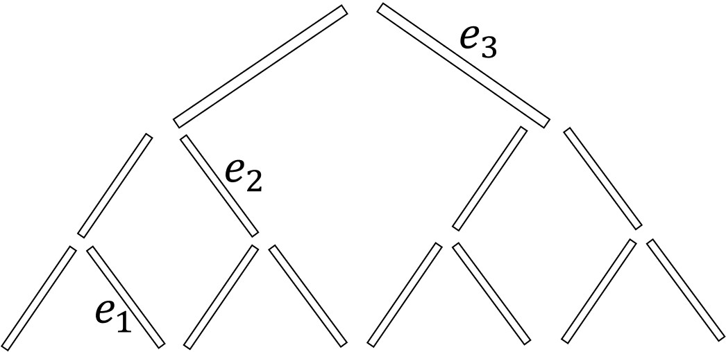
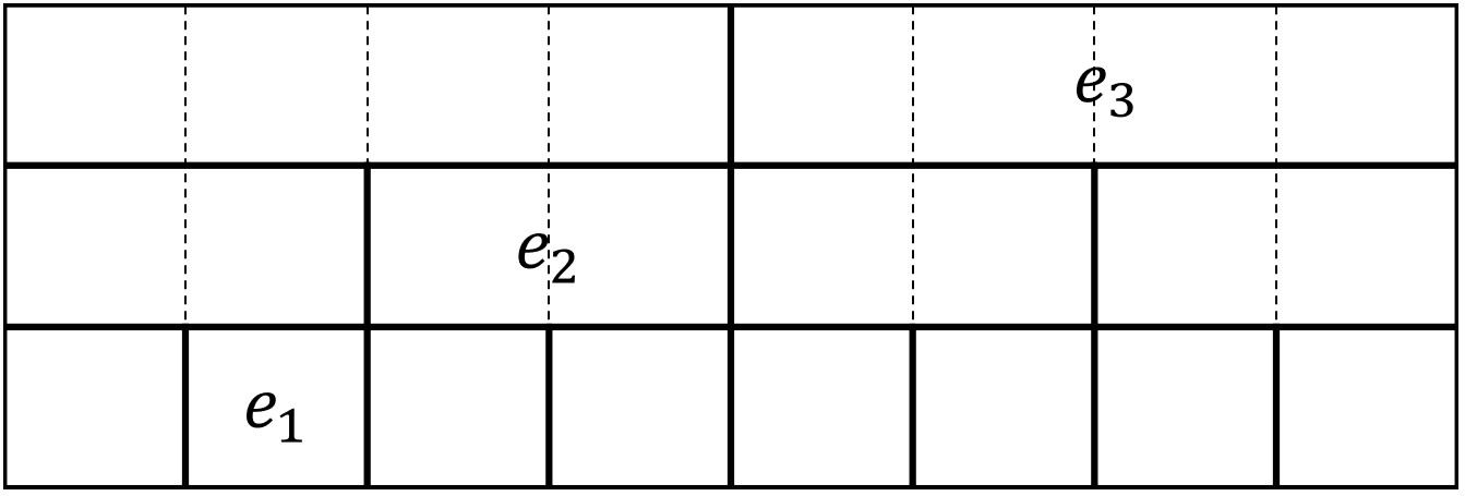
(a)

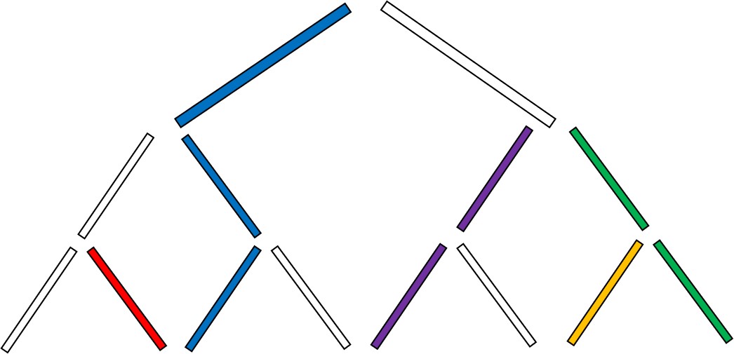
(b)

Figure 2: (a) An example of a binary tree and its corresponding grid; (b) Jobs arrive bottom-up and get allocated. The grid shows the cells marked by each job.

Say an edge $e$ at level $\ell$ is “good” if when the buyers beginning with $e$ start to arrive, we have $(L-\ell)m(e)\geq 2^{\ell}\sqrt{L/\log L}$. For any buyer beginning with a good edge that is allocated by the algorithm, it marks a rectangle in the grid with area $(L-\ell)m(e)\geq\sqrt{L/\log L}\cdot v_{\ell}$, i.e $\sqrt{L/\log L}$ times the value of the buyer. Since the total area of the grid is $L2^{L}$, the total value of buyers with good edges allocated in the algorithm is at most $\frac{1}{\sqrt{L/\log L}}L2^{L}=2^{L}\sqrt{L\log L}$.

Now consider the welfare contributed by buyers at bad edges. At any such bad edge $e$ at level $\ell$, at most $m(e)$ buyers beginning with $e$ can get allocated; the expected number of such buyers that arrive is at most $\frac{m(e)}{2^{\ell}}<\frac{\sqrt{L/\log L}}{L-\ell}$. Thus their total welfare contribution is at most

$$\sum_{\ell=0}^{L-1}n_{\ell}v_{\ell}\cdot\frac{\sqrt{L/\log L}}{L-\ell}=2^{L}\sqrt{L/\log L}\sum_{\ell=0}^{L-1}\frac{1}{L-\ell}=O(2^{L}\sqrt{L\log L}).$$

Summing up the total welfare contribution from buyers at good and bad edges gives us a bound of $O(2^{L}\sqrt{L\log L})$ on the total welfare obtained by any online algorithm. ∎

5 Bundle Pricings for Path Preferences

We now turn to the path preferences setting. Recall that here the items correspond to edges in a fixed tree. Each buyer $i$ desires a path $P_{i}\subset T$. Our techniques for this setting are similar to those in Section 3 — we construct a partition of the items into layers, construct a corresponding fractional allocation that respects this layer structure in that every buyer is allocated items from at most two layers, and no layer has too much fractional weight. We show in Section 5.2 that such a good fractional layered allocation always exists. In Section 5.3 we show that a layered allocation guarantees a good bundle pricing. In Section 5.4 we present the corresponding “large markets” result, namely that the competitive ratio decreases linearly with capacity.

5.1 Fractional layered allocations

As in the case of fractional unit allocations that we defined for the interval preferences setting, we would like to construct a partition of items into bundles and a corresponding allocation of jobs such that each job fits cleanly into one bundle, no bundle contains too much fractional weight, and no item belongs to more bundles than its multiplicity. Unfortunately, it turns out that due to the rich combinatorial structure among paths in trees, such an allocation cannot be constructed without losing too much value in the worst case.

To overcome this issue, we simplify the combinatorial structure by orienting the underlying tree with an arbitrary root and breaking each path into two “monotone” components. Formally, for an arbitrary rooting of the underlying tree, define the depth of an edge $t\in T$, denoted $d(t)$, to be the number of edges on the shortest path from the root to this edge, including $t$ itself. For a job $j$ with corresponding path $P_{j}$, define the peak of $j$’s desired path to be the edge(s) closest to the root: ${\Lambda_{j}}=\operatorname{arg\,min}_{t\in{I_{j}}}\{d(t)\}$. Let ${{j}^{1}}$ and ${{j}^{2}}$ denote the two subpaths of ${I_{j}}$ that begin at one of the peak edges in ${\Lambda_{j}}$ and consist of all subsequent edges in ${I_{j}}$ with increasing depth; we call these the arms of the job. Let $P_{{{j}^{1}}}$ and $P_{{{j}^{1}}}$ denote the corresponding subpaths. Note that one of these arms may be empty; in that case, we take ${{j}^{2}}$ to be the empty arm.

Definition 5.1.

A fractional allocation $x$ is a fractional layered allocation if there exists a partition of the multiset of items (where item $t$ has multiplicity $B_{t}$) into bundles $\{T_{1},T_{2},T_{3},\cdots\}$, and a corresponding partition of the arms with non-zero weight under $x$, $\cup_{j\in U:x_{j}>0}\{{{j}^{1}},{{j}^{2}}\}$, into sets $\{A_{1},A_{2},A_{3},\cdots\}$, such that:

• For all $j\in U$ with $x_{j}>0$, there is exactly one index $k$ with ${{j}^{1}}\subset A_{k}$ and, if ${{j}^{2}}$ is not empty, exactly one index $k^{\prime}$ with ${{j}^{2}}\in A_{k^{\prime}}$.

• For all $k$ and ${{j}^{a}}\in A_{k}$, $P_{{{j}^{a}}}\subseteq T_{k}$.

• For all $k$ and $t\in T_{k}$, we have ${\textsc{FracWt}}(x,\{j:{{j}^{a}}\in A_{k}\text{ and }P_{{{j}^{a}}}\ni t\})\leq 1$.

Observe that there are two main differences between the layered allocations defined above and fractional unit allocations as defined in Section 3.1. First, layered allocations partition arms into layers rather than entire jobs, so a job can end up in two different layers. Second, and more importantly, a layer can have very large total weight. All we guarantee is that the weight of any single edge in a layer will be bounded by $1$. As such, the pricing we construct is allowed to allocate multiple subpaths of a single layer to different buyers in sequence.

5.2 Layering a tree

We now show that good fractional layered allocations always exist. For a fractional allocation $x$, let $v_{\max}(x)=\max_{j:{x_{j}}>0}v_{j}$ and $v_{\min}(x)=\min_{j:{x_{j}}>0}v_{j}$.

Lemma 5.1.

For every feasible fractional allocation $x$, one can efficiently construct a feasible layered fractional allocation $\tilde{y}$ such that

$${\textsc{FracVal}}(x)\leq O\left(\frac{v_{\max}(x)}{v_{\min}(x)}\right){\textsc{FracVal}}(\tilde{y}).$$

Before we proceed we need more notation. For a subset of jobs (or arms) $J$, let $E_{J}$ denote the set of edges collectively desired by those jobs: $E_{J}=\cup_{j\in J}P_{j}$. For an edge $t$, let $\textsc{w}_{t}(x):={\textsc{FracWt}}(x,\{j:P_{j}\ni t\})$ denote the total fractional weight of jobs (or arms) whose paths contain $t$. Likewise, let $\textsc{w}_{t}(x_{A})$ or $\textsc{w}_{t}(x,A)$ denote the fractional weight on $t$ from jobs (or arms) in set $A$.

We construct the layering recursively. Informally, given a fractional allocation $x$, we find a set of jobs $J$ such that the fractional demand on any item desired by a job in $J$ is a constant. That is, for all $t\in E_{J}$, $\textsc{w}_{t}(x,J)\leq c$. We scale the fractional allocation of jobs in $J$ by $1/c$, and take this scaled allocation along with the set $E_{J}$ to be the first layer. We thus obtain a feasible layer, and lose a factor of at most $c$ in fractional value.

However, in order to apply this step recursively and arrive at a feasible layered allocation, we need the remaining fractional solution to be feasible for the items remaining after reducing the capacity of every item in $E_{J}$ by one. Therefore, we need the fractional weight on every edge in $E_{J}$ to decrease by at least 1 (or else to zero) after removing $J$. It may not be possible to find a set $J$ which satisfies both this and the constant-demand condition described above. Instead, we find a set $D$ such that jobs in $J$ and $D$ together account for one unit of demand on every edge in $E_{J}$, and then we drop $D$. Because we drop jobs in $D$ rather than assigning them to a layer, we do not need to ensure that the fractional weight on edges in $E_{D}$ decreases by any particular amount. We pick a set $D$ with small fractional weight relative to that of $J$, so that we can charge its lost fractional value to $J$.

Finally, although we have informally described the argument in terms of jobs, in our formal argument we consider sets of arms. This introduces an extra complication: when we drop the set $D$ of arms, we must also drop their sibling arms. We show that we can do this without losing more than another constant factor in fractional value.

We formalize the recursive step in the following lemma; the proof is deferred to Section 7.

Lemma 5.2.

Given a set $U$ of jobs and a non-zero fractional allocation $y$, there exist sets of arms $J\neq\emptyset$ and $D$ such that

1. $J\cap D=\emptyset$;

2. $J\cap D^{\prime}=\emptyset$, where $D^{\prime}=\{{{j}^{a}}:j^{a^{\prime}}\in D,a\neq a^{\prime}\}$;

3. for all $t\in E_{J}$, $\textsc{w}_{t}(y,J\cup D)\geq\min\{1,\textsc{w}_{t}(y)\}$;

4. for all $t\in E_{J}$, $\textsc{w}_{t}(y,J)\leq 7$; and

5. ${\textsc{FracWt}}(y_{J})\geq 2{\textsc{FracWt}}(y_{D})$.

Furthermore, $J$ and $D$ can be found efficiently.

Proof of Lemma 5.1. Let $E$ denote the multiset of edges, with the given multiplicities, in the given tree. Given a set of arms $U$ and a feasible fractional allocation $x$, we apply Lemma 5.2 to generate the sets of arms $J$ and $D$. Let $D^{\prime}$ be the set of “sibling” arms of arms in $D$. Recall that $E_{J}$ is the set of edges contained in the paths desired by $j\in J$. Let $E^{\prime}=E\setminus E_{J}$, and $x^{\prime}=x-x_{J}-x_{D}-x_{D^{\prime}}$.

First, we observe that $x^{\prime}$ is feasible for the multiset $E^{\prime}$ of edges. This is because on the one hand, the multiplicity of each edge $t$ in $E_{J}$ decreases by 1. On the other hand, $\textsc{w}_{t}(x)-\textsc{w}_{t}(x^{\prime})\geq\textsc{w}_{t}(x,J\cup D)\geq\min\{1,\textsc{w}_{t}(x)\}$ by property iii. in Lemma 5.2. So, either the fractional weight on $t$ decreases by $1$, or it is equal to $0$.

We set $T_{1}=E_{J}$, $\tilde{A}_{1}=J$, $D_{1}=D$, and $D^{\prime}_{1}=D^{\prime}$, and construct the remaining partition of edges and arms by applying Lemma 5.2 recursively to allocation $x^{\prime}$. Observe that our rescursive applications may discard in the form of the sets $D^{\prime}_{k}$ some arms that have previously been included in the sets $\tilde{A}_{k^{\prime}}$ for $k^{\prime}<k$. Define $A_{k}=\tilde{A}_{k}\setminus(\cup_{k^{\prime}}D^{\prime}_{k^{\prime}})$. We then define $\tilde{y}_{j}=x_{j}/7$ for jobs $j$ with arms in $\cup_{k}A_{k}$, and $0$ otherwise. It is now easy to see that $\tilde{y}$ is a fractional layered allocation, where the third property follows from property iv. in Lemma 5.2.

It remains to prove that the fractional value of $\tilde{y}$ is large enough. Property v. in Lemma 5.2 tells us that ${\textsc{FracWt}}(x,\tilde{A}_{k})\geq{\textsc{FracWt}}(x,D_{k}\cup D^{\prime}_{k})$. Summing over $k$ and removing the contribution of $D^{\prime}_{k}$ from each side, we get

$${\textsc{FracWt}}(x,\cup_{k}A_{k})\geq{\textsc{FracWt}}(x,\cup_{k}D_{k})\geq\frac{1}{2}{\textsc{FracWt}}(x,\cup_{k}(D_{k}\cup D^{\prime}_{k})),$$

which implies ${\textsc{FracWt}}(x,\cup_{k}A_{k})\geq\frac{1}{3}{\textsc{FracWt}}(x)$, or ${\textsc{FracWt}}(\tilde{y})\geq\frac{1}{21}{\textsc{FracWt}}(x)$.

Finally, since the values of all jobs with positive weight under $x$ lie in the range $[v_{\min}(x),v_{\max}(x)]$, we get that ${\textsc{FracVal}}(\tilde{y})\geq\Omega\left(\frac{v_{\min}(x)}{v_{\max}(x)}\right){\textsc{FracVal}}(x)$. ∎

5.3 From layered allocations to bundle pricings

In this section we will demonstrate the existence of a good bundle pricing given any fractional layered allocation:

Lemma 5.3.

Given a feasible fractional layered allocation $y$, there exists a bundle pricing $\mathbf{p}$ such that

$${\textsc{FracVal}}(y)\leq O\left(\frac{v_{\max}(y)}{v_{\min}(y)}\right){\textsc{SW}}(\mathbf{p}).$$

To develop intuition for our approach consider the special case where every edge in the tree has capacity $1$ (that is, the layered allocation has a single layer), and every job has equal value. We claim that essentially the most contentious edges in a job’s path are its peak edges – those closest to the root. In particular, if a job gets “blocked” by another admitted job on one or more of its peak edges, then we should try to recover its lost value in the form of revenue from the blocking edge. What if a job gets blocked on a non-peak edge? We can then charge the lost value of this job to the value of the blocking job—it is easy to observe that any such blocking job is charged at most once in this manner. In effect, every job has up to two important edges, namely its peak edges, that determine whether and to what extent the job will contribute to the solution’s revenue or its utility. Upon focusing on these two edges, then, the instance behaves like one where every desired bundle has size $2$ and we can construct a bundle pricing that achieves a competitive ratio of $O(1)$. In order to convert this argument into a proof we need to deal with several complications: jobs have different values; different arms of a job may be allocated at different layers in the fractional layered allocation; etc.

Proof.

We start by introducing some notation. Given the fractional layered allocation $y$, let $\{T_{1},T_{2},\cdots\}$ be the partition of items/edges into layers, and $\{A_{1},A_{2},\cdots\}$ be the corresponding partition of arms. Henceforth we will think of the different copies of an edge as distinct items, and when we refer to some edge/item $e$ it will be understood that this edge corresponds to some particular set $T_{k}$. For a $j\in U$ with $y_{j}>0$, and for the index $k$ such that ${{j}^{a}}\in A_{k}$, we will redefine $P_{{{j}^{a}}}$ (and likewise, $P_{j}$) as the subset of edges of $T_{k}$ that correspond to this arm. Accordingly, we also redefine the peak edges, ${\Lambda_{j}}$, of a job $j$ with $y_{j}>0$ as the copies of its peak edges that belong to $T_{k}$ corresponding to ${{j}^{a}}\in A_{k}$. Note that we may assume without loss of generality (via rescaling, e.g.) that $v_{\min}(y)=1$.

We are now ready to define our pricing:

• For any layer $k$, edge $e\in T_{k}$, and job $j$ such that ${{j}^{a}}\in A_{k}$, define the contribution of $j$ to $e$’s price as $\gamma_{ej}=\frac{1}{4}y_{j}v_{j}\mathbbm{1}[e\in{\Lambda_{j}}]$. For all other pairs $(j,e)$, set $\gamma_{ej}=0$.

• For any $k$ and edge $e\in T_{k}$, define the price of $e$ as $\hat{p}_{e}=\sum_{j}\gamma_{ej}$.

• For any $k$ and a bundle $B\subset T_{k}$ that corresponds to a “monotone” path, define the price of the bundle as $p_{B}=\max(1,\sum_{e\in B}\hat{p}_{e})$. All other bundles are priced at infinity.

Our mechanism offers the static, anonymous bundle prices $\mathbf{p}$ as defined above. Now consider any instantiation of job arrivals. We consider three events related to job $j$:

• $\mathcal{E}^{1}_{j}$ occurs if, at the time of $j$’s arrival, all edges in ${\Lambda_{j}}$ are unsold;

• $\mathcal{E}^{2}_{j}$ occurs if, after all jobs have arrived, at least one of the edges in ${\Lambda_{j}}$ is sold;

• $G_{j}$ occurs when either of the above holds: $G_{j}={\mathcal{E}}^{1}_{j}\cup{\mathcal{E}}^{2}_{j}$.

We now make the following two claims. The first bounds the contribution to the welfare of the pricing from “good” jobs for which event $G_{j}$ occurs. The second bounds the loss from the “bad” jobs. Here ${\textsc{Util}}(\mathbf{p})$ denotes the total buyer utility generated by the pricing $\mathbf{p}$ and ${\textsc{Rev}}(\mathbf{p})$ denotes the total revenue generated.

Claim 1.

$${\textsc{Util}}(\mathbf{p})+4\;{\textsc{Rev}}(\mathbf{p})+{\textsc{SW}}(\mathbf{p})\geq\sum_{j}y_{j}v_{j}\textrm{\bf Pr}\!\left[G_{j}\right]-\frac{1}{2}{\textsc{FracVal}}(y).$$ (4)

Claim 2.

$$2v_{\max}(y){\textsc{SW}}(\mathbf{p})\geq\sum_{j}y_{j}v_{j}\textrm{\bf Pr}\!\left[\mkern 1.5mu\overline{\mkern-1.5muG_{j}\mkern-1.5mu}\mkern 1.5mu\right].$$ (5)

Given the two claims, adding Equations (4) and (5), and using the fact that ${\textsc{SW}}(\mathbf{p})={\textsc{Util}}(\mathbf{p})+{\textsc{Rev}}(\mathbf{p})$, we have

$$(2v_{\max}(y)+5)\;{\textsc{SW}}(\mathbf{p}) \geq\sum_{j}y_{j}v_{j}-\frac{1}{2}{\textsc{FracVal}}(y)=\frac{1}{2}{\textsc{FracVal}}(y)$$

The theorem follows. It remains to prove the claims.

Proof of Claim 1. For a job $j$ with $y_{j}>0$, let $p(j)=\sum_{e\in P_{j}}\hat{p}_{e}$ denote the price of the “intended” bundle for $j$. We first write the utility of the pricing $\mathbf{p}$:

$${\textsc{Util}}(\mathbf{p}) \geq\sum_{j}y_{j}\textrm{\bf Pr}\!\left[\mathcal{E}^{1}_{j}\right]\big{(}v_{j}-\max\{1,p(j)\}\big{)}$$

$$=\sum_{j}y_{j}\textrm{\bf Pr}\!\left[\mathcal{E}^{1}_{j}\right]\big{(}v_{j}-p(j)\big{)}-\sum_{j}y_{j}\textrm{\bf Pr}\!\left[\mathcal{E}^{1}_{j}\right]\big{(}1-p(j)\big{)}^{+}$$

$$=\sum_{j}v_{j}y_{j}\textrm{\bf Pr}\!\left[\mathcal{E}^{1}_{j}\right]-\sum_{j}\big{(}y_{j}\textrm{\bf Pr}\!\left[\mathcal{E}^{1}_{j}\right]\sum_{e\in P_{j}}\hat{p}_{e}\big{)}-\sum_{j}y_{j}\textrm{\bf Pr}\!\left[\mathcal{E}^{1}_{j}\right]\big{(}1-p(j)\big{)}^{+}$$ (6)

where the inequality follows because each job is a profit-maximizer and, when not blocked, will pay the sum of the prices (or 1) if this is less than its value.

We bound the three terms in (6) separately, beginning with the third. Note that job $j$ always purchases some bundle containing its path when it arrives, if event $\mathcal{E}^{1}_{j}$ occurs. Therefore, since $(1-p(j))^{+}\leq 1$ and the single-minded buyer’s value for any bundle containing his path is least 1,

$$\sum_{j}y_{j}\textrm{\bf Pr}\!\left[A_{j}\right]\big{(}1-p(j)\big{)}^{+}\leq{\textsc{SW}}(\mathbf{p}).$$ (7)

For the second term, we have:

$$\sum_{j}\left(y_{j}\textrm{\bf Pr}\!\left[\mathcal{E}^{1}_{j}\right]\sum_{e\in P_{j}}\hat{p}_{e}\right)\leq\sum_{e}\left(\hat{p}_{e}\sum_{j:e\in P_{j}}y_{j}\right) \leq\sum_{e}\hat{p}_{e}$$

$$=\sum_{e,j}\gamma_{e,j}=\sum_{j}\sum_{e\in{\Lambda_{j}}}\frac{1}{4}y_{j}v_{j}\leq\frac{1}{2}{\textsc{FracVal}}(y)$$ (8)

where the second inequality follows from the definition of fractional layered allocations.

We now bound the first term in (6). For edge $e$, let $\mathcal{E}^{2}_{e}$ denote that, after all jobs have arrived, edge $e$ is sold. Recall that $G_{j}=\mathcal{E}^{1}_{j}\cup\mathcal{E}^{2}_{j}=\mathcal{E}^{1}_{j}\cup(\cup_{e\in{\Lambda_{j}}}\mathcal{E}^{2}_{e})$. Therefore,

$$v_{j}y_{j}\mathbbm{1}[G_{j}] \leq v_{j}y_{j}\mathbbm{1}[\mathcal{E}^{1}_{j}]+\sum_{e\in{\Lambda_{j}}}v_{j}y_{j}\mathbbm{1}[\mathcal{E}^{2}_{e}]$$

$$=v_{j}y_{j}\mathbbm{1}[\mathcal{E}^{1}_{j}]+\sum_{e}4\gamma_{ej}\mathbbm{1}[\mathcal{E}^{2}_{e}]$$

Summing over all $$j$$,

$$\sum_{j}v_{j}y_{j}\mathbbm{1}[G_{j}] \leq\sum_{j}v_{j}y_{j}\mathbbm{1}[\mathcal{E}^{1}_{j}]+4\sum_{e}\mathbbm{1}[\mathcal{E}^{2}_{e}]\sum_{j}\gamma_{ej}$$

$$=\sum_{j}v_{j}y_{j}\mathbbm{1}[\mathcal{E}^{1}_{j}]+4\sum_{e}\mathbbm{1}[\mathcal{E}^{2}_{e}]\hat{p}_{e}$$

$$\leq\sum_{j}v_{j}y_{j}\mathbbm{1}[\mathcal{E}^{1}_{j}]+4{\textsc{Rev}}(\mathbf{p})$$ (9)

The claim now follows by putting together Equations (6), (7), (8), and (9). ∎

Proof of Claim 2. Fix a particular instantiation of jobs and consider a job $j$ for which $G_{j}$ does not occur. Then $j$ is blocked at the time of its arrival on some non-peak edge in $P_{j}$. Let $e$ be the edge closest to the root among all such blocking edges. Then, $e$ is a peak edge for the job $j^{\prime}$ that is allocated this edge. We charge the quantity $v_{j}q_{j}$ to $j^{\prime}$.

Now observe that all of the jobs $j$ that are charged to some job $j^{\prime}$ along edge $e\in T_{k}$ contain the parent edge of $e$, call it $e^{\prime}$, in their arm ${{j}^{a}}\in A_{k}$. Then we can use the fact that ${\textsc{FracWt}}(y,\{j:{{j}^{a}}\in A_{k}\text{ and }P_{{{j}^{a}}}\ni e^{\prime}\})\leq 1$ from the definition of fractional layered allocations to assert that the total weight of such jobs is at most $1$. In other words, the total charge on $j^{\prime}$ is at most

$$\sum_{j:j\text{ charges }j^{\prime}}v_{j}q_{j}\leq v_{\max}(y)\sum_{j:j\text{ charges }j^{\prime}}q_{j}\leq 2v_{\max}(y)\leq 2v_{\max}(y)v_{j^{\prime}}$$

where the factor of $2$ arises from the fact that $j^{\prime}$ could be charged along both of its peak edges, and the last inequality follows by recalling that $v_{j^{\prime}}\geq v_{\min}(y)=1$ for any job $j^{\prime}$ allocated by the pricing.

The claim now follows by summing the above inequality over jobs $j^{\prime}$ allocated by the pricing, and taking expectations of both sides over possible instantiations. ∎ This completes the proof of the lemma. ∎

Armed with this lemma, we can now complete the proof of Theorem 1.4. Start with the optimal fractional allocation $y$, and partition all jobs into $\log H$ value classes, where each class contains jobs with values within a factor of $2$ of each other. One of these classes, call it $C$, contributes more than a $\log H$ fraction to the fractional value of $y$. Then, applying Lemma 5.3 to the allocation $y_{C}$ gives us the following theorem.

Theorem 1.4.

For the path preferences setting, there exists a static, anonymous bundle pricing with competitive ratio $O\left(\log H\right)$ for social welfare.

5.4 The large capacity setting

In this section we consider the setting where every edge is available in large supply. Recall that we define $B:=\min_{t}B_{t}$. We show that as $B$ increases, the approximation ratio achieved by bundle pricing gradually decreases.

Theorem 1.5.

For the path preferences setting, if every edge has at least $B>0$ copies available, then a static, anonymous bundle pricing achieves a competitive ratio of $O\left(\frac{1}{B}\log H\right)$ for social welfare.

Proof.

Let $k=\frac{1}{2}B$ and $\alpha=H^{1/k}$. The proof technique is basically identical to that of Theorem 1.2, where we partition both the item supply and the jobs into $k$ instances, such that on the one hand, the fractional solution confined to jobs within an instance will be feasible for the item supply in that instance; on the other hand, within each instance job values will differ by a factor of at most $\alpha$. Then, applying Theorem 1.4 will give us a static, anonymous pricing for every instance individually with a factor of $\Omega\big{(}\frac{1}{\log\alpha}\big{)}$ loss in social welfare. Now consider running these instances in parallel, with each buyer allowed to purchase bundles from any of the instances. The utility-revenue analysis in Lemma 5.3 continues to apply, providing the same guarantees on welfare. However, we may double count some part of the welfare: suppose a buyer $j$ is “assigned” by the layered allocation to one instance, but purchases a bundle in another instance; then we may account for both his contribution to utility for the first instance as well as his contribution to revenue for the second instance. This double counting only costs us a factor of $2$ in the overall welfare, and we obtain an $O(\log\alpha)=O\left(\frac{1}{B}\log H\right)$ approximation. ∎

6 Convex Production Costs with Interval Preferences

In this section we show that our results for interval preferences, in particular Theorems 1.1 and 1.2, generalize to the setting where the seller can obtain additional copies of each item at increasing marginal costs. In particular, we assume the seller incurs cost $c_{ti}$ when allocating the $i$th copy of item $t$, and $c_{ti}\geq c_{ti^{\prime}}$ for $i>i^{\prime}$. Note that this generalizes the fixed-capacity setting by taking $c_{ti}=0$ for $i\leq B_{t}$ and $\infty$ otherwise. We begin by revisiting our definition of fractional allocations and associated notation, which we defined for fixed-capacity settings in Section 2.

In this setting, a fractional allocation $x$ no longer need satisfy an explicit supply constraint, but the fractional value achieved by $x$ is different, since the costs of supply must be taken into account. We begin by introducing notation for the cost of a given fractional allocation. For any fractional allocation $x$, denote by $b_{t}(x)=\sum_{j:{I_{j}}\ni t}x_{j}$ the (fractional) number of copies of item $t$ allocated in $x$. Let $b_{tr}(x)$ be the fraction of copy $r$ of item $t$ sold:

$$b_{tr}(x)=\begin{cases}1&r\leq b_{t}(x)\\ b_{t}(x)-\lfloor b_{t}(x)\rfloor&r=\lfloor b_{t}(x)\rfloor+1\\ 0&r>\lfloor b_{t}(x)\rfloor+1.\end{cases}$$

For simplicity we use $b_{t}$ to denote $b_{t}(x)$ and $b_{tr}$ to denote $b_{tr}(x)$ in later analysis. Observe that the total cost for all copies of item $t$ in $x$ is $\sum_{r}b_{tr}c_{tr}$. Then the fractional value achieved by $x$ is

$${\textsc{FracVal}}(x,\vec{c})=\sum_{j}v_{j}x_{j}-\sum_{t,r}b_{tr}c_{tr}.$$

As in the fixed-capacity setting, we bound the optimal welfare by the optimal fractional welfare; define

$${\textsc{FracOpt}}:=\max_{x}{\textsc{FracVal}}(x,\vec{c}),$$

where $x$ ranges over $x\geq 0$ satisfying the demand constraint (Equation 2). We defer our proof of Lemma 6.1 to Section 7.

Lemma 6.1.

${\textsc{FracOpt}}_{\vec{c}}\geq{\textsc{Opt}}_{\vec{c}}$.

We now show that our analysis (theorems in Section 3 along with Lemma 3.1) extends to the setting with convex production costs as well. We begin by updating our definition of fractional unit allocations. Recall that unit allocations implicitly define a partition of items into bundles and associate each job with at most one bundle. When items have production costs, the value of a fractional unit allocation depends on which copy of each item belongs to any particular bundle in the partition. This association of copies to bundles is not necessarily unique. So we extend the definition of unit allocations to make the partitioning of items into bundles explicit.

Definition 6.1.

A fractional unit allocation with costs is a pair $(x,\tau)$, where $x$ is a demand-feasible fractional allocation and $\tau=\{\tau_{1},\tau_{2},\tau_{3},\cdots\}$ is a partition of the multiset of items $\{(t,r)\}_{t\in T,r\in\mathbb{Z}^{+}}$, if there exists a partition of jobs $j\in U$ with $x_{j}>0$ into sets $\{A_{1},A_{2},A_{3},\cdots\}$, such that:

• For all $k$, the set of items contained in $\tau_{k}$, $T_{k}=\{t:(t,r)\in\tau_{k}\}$, forms an interval.

• For all $j\in U$ with $x_{j}>0$, there is exactly one index $k$ with $j\in A_{k}$.

• For all $k$ and $j\in A_{k}$, $I_{j}\subseteq T_{k}$.

• For all $k$, we have ${\textsc{FracWt}}(x_{A_{k}})\leq 1$.

The fractional value of $(x,\tau)$ is defined as:

$${\textsc{FracVal}}(x,\tau,\vec{c})=\sum_{j}v_{j}x_{j}-\sum_{k}\sum_{(t,r)\in\tau_{k}}\sum_{j\in A_{k}:t\in I_{j}}c_{tr}x_{j}.$$

We can now state a counterpart to Lemma 3.1, with the proof deferred to Section 7.

Lemma 6.2.

For any cost vector $\vec{c}$ and a fractional unit allocation with costs, $(x,\tau)$, there exists an anonymous bundle pricing $\mathbf{p}$ such that

$${\textsc{SW}}(\mathbf{p})\geq\frac{1}{2}{\textsc{FracVal}}(x,\tau,\vec{c}).$$

We emphasize that the pricing returned by the above lemma is not necessarily static. For each bundle $\tau_{k}$ in the unit allocation $(x,\tau)$, our pricing associates a price with each interval $I\subseteq T_{k}$. Prices for different such subsets $I$ can be different and depend on the costs of the respective items. When one of the intervals in $\tau_{k}$ is bought, the seller removes from the menu all other intervals corresponding to $\tau_{k}$. Moreover, different copies of the same bundle can have different prices, because they cost different amounts to the seller. We leave open the question of obtaining a static bundle pricing with a good approximation factor for this setting.

Next we state and prove a counterpart of Theorem 3.11: given any fractional allocation $x$ we can construct a fractional unit allocation that captures an $O(\log L/\log\log L)$ fraction of the value of $x$. The proof is essentially a reduction to the fixed-capacity setting. We first partition the allocation $x$ into “layers” as in the proof of Theorem 3.11. The fractional weight for every item in the allocation for any single layer is at most 1. In this case, it becomes possible to apply the unit-capacity theorem (Theorem 3.10) to construct a partition of items in that layer and a corresponding unit allocation. Putting these layer-by-layer unit-allocations together gives us an overall fractional unit allocation.

Lemma 6.3.

For all non-decreasing costs $\vec{c}$ and every fractional allocation $x$, there exists a fractional unit allocation $(x^{\prime},\tau)$ such that

$${\textsc{FracVal}}(x,\vec{c})\leq O(\log L/\log\log L){\textsc{FracVal}}(x^{\prime},\tau,\vec{c}).$$

Lemmas 6.1, 6.2 and 6.3 together imply the following upper bound for the costs setting.

Theorem 6.4.

For the interval preferences setting with increasing marginal costs on items, there exists an anonymous bundle pricing $\mathbf{p}$ such that

$${\textsc{Opt}}\leq O\left(\frac{\log L}{\log\log L}\right){\textsc{SW}}(\mathbf{p}).$$

The lower bound of $\Omega\left(\frac{\log L}{\log\log L}\right)$ also extends to the setting with costs, as the unit-capacity setting is a special case.

7 Deferred proofs

7.1 Proof of Lemma 3.1

Lemma 3.1.

For any feasible fractional unit allocation $x$, there exists a static, anonymous bundle pricing $\mathbf{p}$ such that

$${\textsc{SW}}(\mathbf{p})\geq\frac{1}{2}{\textsc{FracVal}}(x).$$

Proof.

Observe that we can write the social welfare of any $\mathbf{p}$ as the sum of the expected revenue of the seller and the total expected utility obtained by the buyers:

$${\textsc{SW}}(p)={\textsc{Rev}}(p)+{\textsc{Util}}(p).$$

Let $\{T_{k}\}$ and $\{A_{k}\}$ be the partition of the items and jobs respectively corresponding to the unit allocation $x$. For each bundle $T_{k}$, let $W_{k}={\textsc{FracWt}}(x_{A_{k}})$, and set price ${p_{k}}=\frac{1}{2W_{k}}{\textsc{FracVal}}(x_{A_{k}})$. For this setting of prices, we will bound the revenue and utility terms separately, and show that their sum is at least $\frac{1}{2}{\textsc{FracVal}}(x)=\frac{1}{2}\sum_{k}{\textsc{FracVal}}(x_{A_{k}})$.

For any realization of the buyers’ values and arrival order, let $Z_{k}$ indicate whether bundle $k$ is purchased by any buyer at these prices. The revenue term is then

$${\textsc{Rev}}(p) =\sum_{k}\Pr[Z_{k}=1]{p_{k}}$$

$$\geq\frac{1}{2}\sum_{k}\Pr[Z_{k}=1]{\textsc{FracVal}}(x_{A_{k}}).$$ (10)

The inequality follows from the fact that $W_{k}\leq 1$ by the definition of unit allocations.

For the utility, note that buyer $i$ with value $v_{i}$ will purchase an available bundle maximizing her utility. Define $k_{j}$ to be the index $k$ such that $j\in A_{k}$. The buyer’s utility is at least

$$u_{i}(v_{i}) \geq\textrm{\bf E}_{Z}\!\left[\max_{j\in J_{v_{i}}}\mathbbm{1}\{Z_{k_{j}}=0\}\big{(}v_{i}({I_{j}})-p_{k_{j}}\big{)}^{+}\right]$$

$$\geq\frac{1}{{q_{v_{i}}}}\sum_{j\in J_{v_{i}}}\Pr[Z_{k_{j}}=0]{x_{j}}(v_{j}-p_{k_{j}})^{+}.$$ (11)

The second inequality follows from (2).

Summing over all buyers and all valuations, we have

$${\textsc{Util}}(p) \geq\sum_{i,v_{i}}{q_{v_{i}}}u_{i}(v_{i})$$

$$\geq\sum_{i,v_{i}}\sum_{j\in J_{v_{i}}}\Pr[Z_{k_{j}}=0]{x_{j}}(v_{j}-p_{k_{j}})^{+}$$

$$\geq\sum_{k}\Pr[Z_{k}=0]\sum_{j\in A_{k}}{x_{j}}(v_{j}-{p_{k}})$$

$$\geq\sum_{k}\Pr[Z_{k}=0]\Big{(}{\textsc{FracVal}}(x_{A_{k}})-W_{k}{p_{k}}\Big{)}$$

$$\geq\sum_{k}\Pr[Z_{k}=0]\Big{(}{\textsc{FracVal}}(x_{A_{k}})-\frac{1}{2}{\textsc{FracVal}}(x_{A_{k}})\Big{)}$$

$$=\frac{1}{2}\sum_{k}\Pr[Z_{k}=0]{\textsc{FracVal}}(x_{A_{k}})$$ (12)

The result now follows by summing (10) and (12). ∎

7.2 Proof of Lemma 3.2

Lemma 3.2.

For any fractional allocation $x$, there exists a set of jobs $U_{1}$ as defined in Section 3.2 such that ${\textsc{FracVal}}(x_{U_{1}})\geq\frac{1}{2}{\textsc{FracVal}}(x)$.

Proof.

We bound the total fractional value of jobs left out of $U_{1}$:

$$\sum_{j\not\in U_{1}}v_{j}x_{j} <\sum_{j\not\in U_{1}}\left(\frac{1}{2}\sum_{t\in I_{j}}\textsc{val}_{t}\right)x_{j}$$

$$=\frac{1}{2}\sum_{j\not\in U_{1}}x_{j}\left(\sum_{t\in I_{j}}\sum_{j^{\prime}:I_{j^{\prime}}\ni t}\rho_{j^{\prime}}x_{j^{\prime}}\right)$$

$$=\frac{1}{2}\sum_{t}\left(\sum_{\begin{subarray}{c}j\not\in U_{1}\\ I_{j}\ni t\end{subarray}}x_{j}\right)\sum_{j^{\prime}:I_{j^{\prime}}\ni t}\rho_{j^{\prime}}x_{j^{\prime}}$$

$$\leq\frac{1}{2}\sum_{t}\sum_{j:I_{j}\ni t}\rho_{j}x_{j}=\frac{1}{2}{\textsc{FracVal}}(x).$$

∎

7.3 Proof of Lemma 3.8

Lemma 3.8.

For each interval ${\mathbbm{I}}_{\ell,k}$, there exists a set of jobs $S_{\ell,k}\subseteq{\tilde{G}}_{\ell,k}$ such that

1. ${\textsc{FracWt}}(x,S_{\ell,k})\leq\frac{1}{\beta}$ and

2. ${\textsc{FracVal}}(x,S_{\ell,k})\geq\frac{1}{6}{\textsc{FracVal}}(x,{\tilde{G}}_{\ell,k})$.

Proof.

Since all jobs in ${\tilde{G}}_{\ell,k,a}$ have value between $2^{a-1}$ and $2^{a}$, we have

$$2^{a-1}{\textsc{FracWt}}(x,{\tilde{G}}_{\ell,k,a})\leq{\textsc{FracVal}}(x,{\tilde{G}}_{\ell,k,a})\leq 2^{a}{\textsc{FracWt}}(x,{\tilde{G}}_{\ell,k,a}).$$

For every $u\in\{1,\cdots,\lceil\log v_{\max}\rceil\}$, define $S_{u}=\sum_{a\leq u}2^{a}{\textsc{FracWt}}(x,{\tilde{G}}_{\ell,k,a})$. Then $S_{\lceil\log v_{\max}\rceil}$ is an upperbound of ${\textsc{FracVal}}(x,{\tilde{G}}_{\ell,k})$. Let $m$ be such that $S_{m}\leq\frac{1}{3}S_{\lceil\log v_{\max}\rceil}$ and $S_{m+1}>\frac{1}{3}S_{\lceil\log v_{\max}\rceil}$. Consider the following two cases.

Case 1. If $S_{m+1}-S_{m}=2^{m+1}{\textsc{FracWt}}(x,{\tilde{G}}_{\ell,k,m+1})>\frac{1}{3}S_{\lceil\log v_{\max}\rceil}$, then

$${\textsc{FracVal}}(x,{\tilde{G}}_{\ell,k,m+1}) \geq 2^{m}{\textsc{FracWt}}(x,{\tilde{G}}_{\ell,k,m+1})$$

$$>\frac{1}{6}S_{\lceil\log v_{\max}\rceil}$$

$$\geq\frac{1}{6}{\textsc{FracVal}}(x,{\tilde{G}}_{\ell,k}).$$

Since ${\textsc{FracWt}}(x,{\tilde{G}}_{\ell,k,m+1})\leq\frac{1}{2\beta}<\frac{1}{\beta}$, setting $S_{\ell,k}={\tilde{G}}_{\ell,k,m+1}$ satisfies both conditions of the lemma.

Case 2. If $S_{m+1}-S_{m}\leq\frac{1}{3}S_{\lceil\log v_{\max}\rceil}$, then $S_{m+1}\leq\frac{2}{3}S_{\lceil\log v_{\max}\rceil}$, and

$$\sum_{a>m+1}{\textsc{FracVal}}(x,{\tilde{G}}_{\ell,k,a}) \geq\frac{1}{2}(S_{\lceil\log v_{\max}\rceil}-S_{m+1})$$

$$\geq\frac{1}{6}S_{\lceil\log v_{\max}\rceil}$$

$$\geq\frac{1}{6}{\textsc{FracVal}}(x,{\tilde{G}}_{\ell,k}).$$

Meanwhile, note that $\sum_{a>m+1}2^{a}{\textsc{FracWt}}(x,{\tilde{G}}_{\ell,k,a})<\frac{2}{3}S_{\lceil\log v_{\max}\rceil}<2S_{m+1}.$ Then

$$\sum_{a>m+1}{\textsc{FracWt}}(x,{\tilde{G}}_{\ell,k,a}) \leq\frac{1}{2^{m+2}}\sum_{a>m+1}2^{a}{\textsc{FracWt}}(x,{\tilde{G}}_{\ell,k,a})$$

$$<\frac{1}{2^{m+2}}\cdot 2S_{m+1}$$

$$=\frac{1}{2^{u+1}}\sum_{a\leq m+1}2^{a}{\textsc{FracWt}}(x,{\tilde{G}}_{\ell,k,a})$$

$$\leq\frac{1}{2^{u+1}}\sum_{a\leq m+1}2^{a}\frac{1}{2\beta}<\frac{1}{\beta}.$$

Thus setting $S_{\ell,k}=\bigcup_{a>m+1}{\tilde{G}}_{\ell,k,a}$ satisfies both conditions of the lemma. ∎

7.4 Proof of Lemma 3.9

Lemma 3.9.

There exists a fractional unit allocation $\tilde{x}_{\mathcal{L}}$ such that

$$\sum_{G\in{\mathcal{L}}}{\textsc{FracVal}}(x_{G})\leq O\left(\frac{\log L}{\log\beta}\right){\textsc{FracVal}}(\tilde{x}_{\mathcal{L}}).$$

Proof.

Fix any length scale $\ell$ and consider the partition of items into intervals ${\mathbbm{I}}_{\ell,k}$. We will construct a fractional unit allocation corresponding to this partition. We first associated with the interval ${\mathbbm{I}}_{\ell,k}$ the set of all jobs contained inside this interval that have length scale between $\ell-\log\beta+1$ and $\ell$. Formally, we define

$$H_{\ell,k}=\bigcup_{\begin{subarray}{c}\ell^{\prime},k^{\prime}:{\mathbbm{I}}_{\ell^{\prime},k^{\prime}}\subseteq{\mathbbm{I}}_{\ell,k}\\ \ell^{\prime}\in(\ell-\log\beta,\ell]\end{subarray}}S_{\ell^{\prime},k^{\prime}},$$

where $S_{\ell^{\prime},k^{\prime}}$ is defined in Lemma 3.8. See Figure 3 for a graphical illustration of $H_{\ell,k}$. Let $H_{\ell}=\cup_{k}H_{\ell,k}$ denote the set of all jobs that belong to the partition given by $\{H_{\ell,k}\}$.

Figure 3: Intervals associated with $H_{\ell,k}$ in Lemma 3.9. There are $\beta-1$ intervals in the block, and from each interval ${\mathbbm{I}}_{\ell^{\prime},k^{\prime}}\subseteq{\mathbbm{I}}_{\ell,k}$ we pick a set of jobs $S_{\ell^{\prime},k^{\prime}}$ with fractional weight at most $1/\beta$.

We now claim that $x_{H_{\ell}}$ is a fractional unit allocation. To see this, observe that for each $(\ell,k)$ there are exactly $2^{\log\beta}-1<\beta$ pairs $(\ell^{\prime},k^{\prime})$ with ${\mathbbm{I}}_{\ell^{\prime},k^{\prime}}\subseteq{\mathbbm{I}}_{\ell,k}$ and $\ell^{\prime}\in(\ell-\log\beta,\ell]$. $H_{\ell,k}$ is therefore a union of at most $\beta$ groups $S_{\ell^{\prime},k^{\prime}}$. Lemma 3.8 now implies that ${\textsc{FracWt}}(x,H_{\ell,k})\leq\beta\frac{1}{\beta}=1$.

Lemma 3.8 also implies that the total fractional value captured by $x_{H_{\ell}}$ is a constant fraction of the total value of all light weight groups at length scales in $(\ell-\log\beta,\ell]$:

$${\textsc{FracVal}}(x,H_{\ell})=\sum_{k}{\textsc{FracVal}}(x,H_{\ell,k}) =\sum_{k}\sum_{\ell^{\prime}\in(\ell-\log\beta,\ell]}{\textsc{FracVal}}(x,S_{\ell^{\prime},k})$$

$$\geq\frac{1}{6}\sum_{k}\sum_{\ell^{\prime}\in(\ell-\log\beta,\ell]}{\textsc{FracVal}}(x,{\tilde{G}}_{\ell^{\prime},k})$$

$$=\frac{1}{6}\sum_{\begin{subarray}{c}G\in{\mathcal{L}};\\ G\text{ at length scale }\ell^{\prime}\in(\ell-\log\beta,\ell]\end{subarray}}{\textsc{FracVal}}(x_{G})$$

Now consider the $\lceil{\ell_{\max}}/\log\beta\rceil$ length scales in $\{1,\cdots,{\ell_{\max}}\}$ that are multiples of $\log\beta$. By our argument above, the fractional allocations $x_{H_{\ell}}$ corresponding to such length scales together capture a sixth of all of the fractional value in ${\mathcal{L}}$. Therefore, there exists some $\ell$ such that

$${\textsc{FracVal}}(x,H_{\ell})\geq\Omega\left(\frac{\log\beta}{{\ell_{\max}}}\right)\sum_{G\in{\mathcal{L}}}{\textsc{FracVal}}(x_{G}).$$

The corresponding unit allocation $x_{H_{\ell}}$ satisfies the requirements of the lemma. ∎

7.5 Proof of Lemma 3.12

Lemma 3.12.

For any feasible fractional allocation $x$ in the interval preferences setting with arbitrary capacities, one can efficiently construct a set $S$ of jobs such that the total fractional weight of $x_{S}$ at any item $t$ is at least $\min\{1,B_{t}\}$ and at most $4$. Formally, for all items $t$, $\min\{1,B_{t}\}\leq\sum_{j\in S:t\in{I_{j}}}x_{j}<4$.

Proof.

We build up the set $S$ greedily as follows. On each iteration, starting from the earliest item $t$ which is not fully covered, we add the job whose interval contains $t$ and ends the latest. More formally, let $S_{0}=\emptyset$. For any set $S$, let $(x,S)|_{t}:=\sum_{j\in S:{I_{j}}\ni t}x_{j}$. On iteration $i$, find $t_{i}=\min\{t:(x,S_{i-1})|_{t}<\min(1,B_{t})\}$. Find $j_{i}=\operatorname{arg\,max}\{t\in{I_{j}}:j\not\in S_{i-1},t_{i}\in{I_{j}}\}$, and set $S_{i}=S_{i-1}\cup\{j_{i}\}$. Let $S=S_{i^{*}}$, where $i^{*}$ is the last iteration.

By construction, $\min\{1,B_{t}\}\leq\sum_{j\in S:t\in{I_{j}}}x_{j}$ for all $t$. Suppose, by way of contradiction, that there exists $t^{\prime}$ such that $\sum_{j\in S:t^{\prime}\in{I_{j}}}x_{j}\geq 4$. Let $\{j_{1},j_{2},\cdots\}\subseteq S$ be all jobs in $S$ containing $t^{\prime}$, indexed in the order in which they were added to $S$. Let $a$ be such that $1\leq\sum_{i=1}^{a}x_{j_{i}}<2$, and let $U_{<}=\{j_{1},\cdots,j_{a}\}$. Similarly, sort the jobs such that they are indexed in order by decreasing end time; let $b$ be such that $1\leq\sum_{i=1}^{b}x_{j_{i}}<2$, and let $U_{>}=\{j_{1},\cdots,j_{b}\}$. Note that $\sum_{j\in U_{<}\cup U_{>}}x_{j}<4$, so there exists a job $j^{\prime}$ which is not in either $U_{<}$ or $U_{>}$. This job was added to $S$ after all jobs in $U_{<}$ were added, and it ends before all jobs in $U_{>}$. Let $i^{\prime}$ be the iteration on which $j^{\prime}$ was added to $S$; we will show there is no item $t_{i^{\prime}}$ for which the algorithm would have added $j^{\prime}$.

Observe that, because the algorithm covers items starting with the earliest uncovered item first, at every iteration $i$ the set of covered items (i.e., the set $\{t:(x,S_{i-1})|_{t}\geq\min(1,B_{t})\}$) is a prefix of $T$, the set of all items. Therefore, by the time the algorithm has added $U_{<}$ to $S$, all items up to and including $t^{\prime}$ have been covered. So $t_{i^{\prime}}$ cannot come before or be equal to $t^{\prime}$. But all jobs in $U_{>}$ contain item $t^{\prime}$, and therefore must have been added to $S$ before job $j^{\prime}$ because they end later. So item $t_{i^{\prime}}$ cannot come after $t^{\prime}$. Therefore job $j^{\prime}$ cannot have been added to $S$. ∎

7.6 Proof of Lemma 5.2

Lemma 5.2.

Given a set $U$ of jobs and a non-zero fractional allocation $y$, there exist sets of arms $J\neq\emptyset$ and $D$ such that

1. $J\cap D=\emptyset$;

2. $J\cap D^{\prime}=\emptyset$, where $D^{\prime}=\{{{j}^{a}}:j^{a^{\prime}}\in D,a\neq a^{\prime}\}$;

3. for all $t\in E_{J}$, $\textsc{w}_{t}(y,J\cup D)\geq\min\{1,\textsc{w}_{t}(y)\}$;

4. for all $t\in E_{J}$, $\textsc{w}_{t}(y,J)\leq 7$; and

5. ${\textsc{FracWt}}(y_{J})\geq 2{\textsc{FracWt}}(y_{D})$.

Furthermore, $J$ and $D$ can be found efficiently.

Proof.

If $\textsc{w}_{t}(y)\leq 6$ for all $t\in T$, then set $J=U$ and $D=\emptyset$. This satisfies the conditions. So assume that there exists $t$ such that $\textsc{w}_{t}(y)>6$. Pick such a $t$ with maximal depth $d(t)$. Thus, for all $t^{\prime}$ in the subtree below $t$, $\textsc{w}_{t^{\prime}}(y)\leq 6$.

Suppose there is a set of arms $S$ which begin at or above $t$ and terminate at $t$ such that $\textsc{w}_{t}(y,S)>3$. Define the depth of an arm to be the depth of the highest edge in its desired interval, so that arms with low depth desire intervals beginning higher in the tree. Then let ${{j_{1}}^{a}},{{j_{2}}^{a}},\cdots,{{j_{k}}^{a}},\cdots,{{j_{\ell}}^{a}}$ be a subset of $S$ sorted in decreasing order by depth such that

$$\sum_{i=1}^{\ell-1}y_{{{j_{i}}^{a}}}<3\leq\sum_{i=1}^{\ell}y_{{{j_{i}}^{a}}}$$

and

$$\sum_{i=k+1}^{\ell}y_{{{j_{i}}^{a}}}<1\leq\sum_{i=k}^{\ell}y_{{{j_{i}}^{a}}}.$$

Then let $J=\{{{j_{1}}^{a}},\cdots,{{j_{k}}^{a}}\}$ and $D=\{{{j_{k+1}}^{a}},\cdots,{{j_{\ell}}^{a}}\}$. Because we are considering arms which terminate at $t$, ${I_{{{j_{i}}^{a}}}}\subseteq{I_{{{j_{i+1}}^{a}}}}$ for all $i\in[\ell-1]$. In particular, $\textsc{w}_{e}(y,J\cup D)\geq\sum_{i=k}^{\ell}y_{{{j_{i}}^{a}}}\geq 1$ for all $e\in T_{J}$. Observe that ${\textsc{FracWt}}(y_{J})\geq 2{\textsc{FracWt}}(y_{D})$. This satisfies the conditions of the lemma.

Suppose there is no set $S$ of arms terminating at $t$ such that $\textsc{w}_{t}(y,S)>3$. Then there must exist a set of arms including $t$ but terminating below $t$ with total weight at least $3$. Let $t_{1},\cdots,t_{d}$ be the $d$ edges below $t$. Let $S_{i}$ be the set of arms that contain both $t$ and $t_{i}$, and $T_{i}$ be the set of arms containing only edges within the subtree planted at $t_{i}$. Because $\textsc{w}_{t_{i}}(y,S_{i})\leq 6$ for all $i$ by our choice of $t$, we can find $m$ such that $3\leq\sum_{i=1}^{m}\textsc{w}_{t}(y,S_{i})<9$. Let $S=\bigcup_{i=1}^{m}S_{i}$. Let $c=\textsc{w}_{t}(y,S)$, so $3\leq c<9$. Let ${{j_{1}}^{a}},\cdots,{{j_{k}}^{a}},\cdots,{{j_{\ell}}^{a}}$ be the arms in $S$ sorted in decreasing order by depth, as before, where

$$2\sum_{i=k+1}^{\ell}y_{{{j_{i}}^{a}}}\leq\sum_{i=1}^{k}y_{{{j_{i}}^{a}}}\leq 7$$

and

$$\sum_{i=k}^{\ell}y_{{{j_{i}}^{a}}}\geq 1.$$

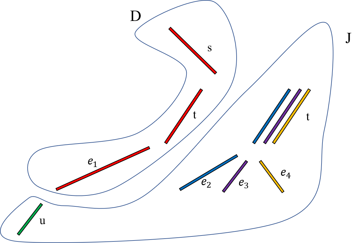
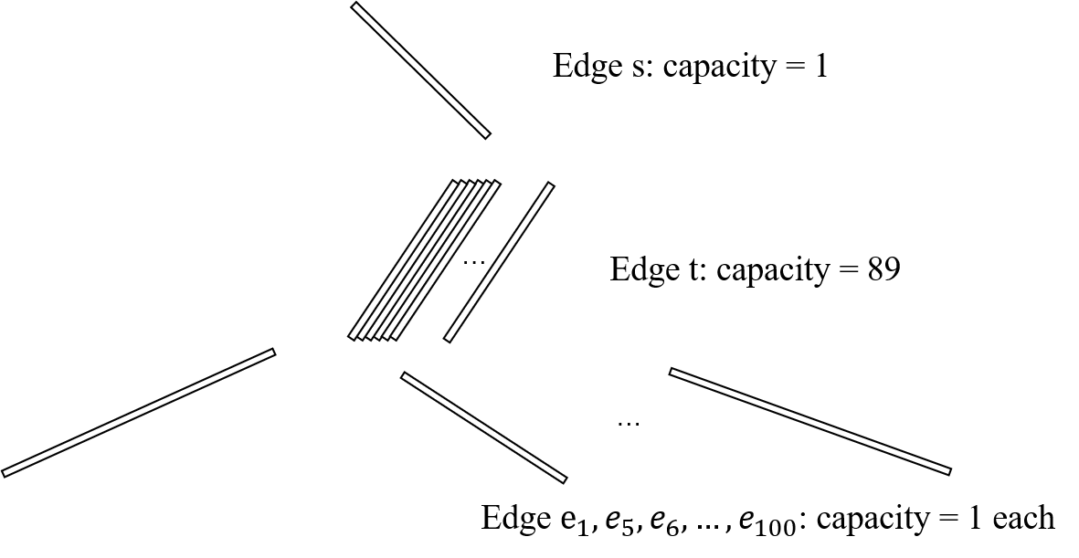
Figure 4: An example for one step of layering algorithm. (Left figure:) At the beginning of the layering step, there are 101 jobs: $(s-t-e_{1})$, $(t-e_{2})$, $(t-e_{3})$, $\cdots$, $(t-e_{100})$, $(u)$. Each job has value 1 and allocation 0.9. The capacity of edge t is 90, while the capacity of other edges are 1. (Middle figure:) In the first step of the layering process, job $(s-t-e_{1})$ is in set $D$, jobs $(t-e_{2})$, $(t-e_{3})$, $(t-e_{3})$ and $(u)$ are in set $J$. The job in set $D$ is deleted, while the jobs in set $J$ have their weight scaled down and allocated to one layer. (Right figure:) The capacity of edges after the first step of layering procedure. The capacity of edges that have positive weight in set $J$ are decreased by 1.

Then set $J=\{{{j_{i}}^{a}}:i=1,\cdots,k\}\cup T_{1}\cup\cdots\cup T_{m}$ and $D=\{{{j_{i}}^{a}}:i=k+1,\cdots,\ell\}$. For each edge $e\in T_{J}$, $\textsc{w}_{t}(y,J)\leq 7$. The same as in previous case for each edge $e$ that is not below $t$, $\textsc{w}_{e}(y,J\cup D)\geq\sum_{i=k}^{\ell}y_{{{j_{i}}^{a}}}\geq 1$; for each edge $e$ below $t$ in $T_{J}$, $\textsc{w}_{e}(y,J\cup D)=\textsc{w}_{t}(y)$. ${\textsc{FracWt}}(y_{J})\geq\sum_{i=1}^{k}y_{{{j_{i}}^{a}}}\geq 2\sum_{i=k+1}^{\ell}y_{{{j_{i}}^{a}}}={\textsc{FracWt}}(y_{D})$. Thus every condition of the lemma is satisfied. ∎

7.7 Proof of Lemma 6.1

Lemma 6.1.

${\textsc{FracOpt}}_{\vec{c}}\geq{\textsc{Opt}}_{\vec{c}}$.

Proof.

Let $x^{*}_{j}$ be the probability that job $j$ is allocated in optimal offline allocation, where the randomness is over all possible realizations of the values. Then $x^{*}$ is a fractional allocation of jobs. Let $d_{tr}$ be the probability that the $r$th copy of item $t$ is allocated in offline optimal allocation. Then $0\leq d_{tr}\leq 1$, $b_{t}(x^{*})=\sum_{r}d_{tr}$,

$${\textsc{Opt}}_{\vec{c}}=\sum_{j}v_{j}x^{*}_{j}-\sum_{t,r}d_{tr}c_{tr}.$$

To prove the lemma, it suffices to show that ${\textsc{FracVal}}(x^{*},\vec{c})\geq{\textsc{Opt}}_{\vec{c}}$, which is equivalent to proving $\sum_{t,r}b_{tr}c_{tr}\leq\sum_{t,r}d_{tr}c_{tr}$. This is true since for every $t$ and $k$, $\sum_{r\geq k}d_{tr}\geq\sum_{r\geq k}b_{tr}$, and

$$\sum_{r\geq 1}d_{tr}c_{tr} = c_{t1}\sum_{r\geq 1}d_{tr}+(c_{t2}-c_{t1})\sum_{r\geq 2}d_{tr}+(c_{t3}-c_{t2})\sum_{r\geq 3}d_{tr}+\cdots$$

$$\geq c_{t1}\sum_{r\geq 1}b_{tr}+(c_{t2}-c_{t1})\sum_{r\geq 2}b_{tr}+(c_{t3}-c_{t2})\sum_{r\geq 3}b_{tr}+\cdots=\sum_{r\geq 1}b_{tr}c_{tr}.$$

∎

7.8 Proof of Lemma 6.2

Lemma 6.2.

For any cost vector $\vec{c}$ and a fractional unit allocation with costs, $(x,\tau)$, there exists an anonymous bundle pricing $\mathbf{p}$ such that

$${\textsc{SW}}(\mathbf{p})\geq\frac{1}{2}{\textsc{FracVal}}(x,\tau,\vec{c}).$$

Proof.

We will give a reduction to the fixed-capacity setting without costs and apply Lemma 3.1. Recall that in a fractional unit allocation with costs, each job $j$ with $x_{j}>0$ is explicitly associated with a particular bundle, and each bundle is explicitly associated with a particular copy of each item contained in the bundle. Thus, the allocation defines a unique charging of the total cost to individual jobs. We construct a pricing instance in the fixed-capacity setting by subtracting from each job’s value the cost of serving it. That is, for every job $j$ in the instance with costs, we construct a job $j^{\prime}$ in the instance without costs with value

$$v_{j^{\prime}}=v_{j}-\sum_{t\in I,(t,r)\in\tau_{k}}c_{tr},$$

where $k$ is such that $j\in A_{k}$ (i.e., the fractional unit allocation with costs assigns job $j$ to bundle $k$). Thus the two instances have identical fractional values, i.e. ${\textsc{FracVal}}^{\prime}(x)={\textsc{FracVal}}(x,\tau,\vec{c})$. By Lemma 3.1, there exists a static, anonymous bundle pricing $\mathbf{p}^{\prime}$ such that

$${\textsc{SW}}^{\prime}(\mathbf{p}^{\prime})\geq\frac{1}{2}{\textsc{FracVal}}^{\prime}(x),$$

and each set $\tau_{k}$ is assigned a price $p^{\prime}_{k}$. We use this bundle pricing to associate the following prices $\mathbf{p}$ to the original instance with costs. For each bundle $\tau_{k}$, for each interval $I\subseteq T_{k}$, set price

$$p_{\tau_{k},I}=p^{\prime}_{k}+\sum_{t\in I,(t,r)\in\tau_{k}}c_{tr}.$$

We refer to the price $p^{\prime}_{k}$ as the base price for bundle $\tau_{k}$, and the sum over costs as the surcharge for interval $I$.

Our menu lists a price for every subinterval of every bundle, covering every copy of every item. However, the mechanism sells at most one interval per bundle: when a buyer selects her preferred interval, the mechanism removes all intervals corresponding to the same bundle from the menu. Thus, our menu is adaptive (prices of unsold intervals change in response to demand for other intervals), though it remains anonymous.

We now claim that the social welfare generated by pricing $\mathbf{p}$ in the instance with costs is precisely equal to the social welfare generated by pricing $\mathbf{p}^{\prime}$ for the new fixed-capacity instance. We prove this pointwise by coupling the buyers’ values and arrival order in the two settings, and then by induction over the number of buyers that have already arrived. Our inductive hypothesis is that at any point of time, the set of bundles available in the new instance is exactly the same as the set of unsold bundles in the original instance. By the way we construct buyers’ values in the new instance, buyers’ preferences over bundles in the two instances are exactly coupled. Thus, the buyers’ total utility is the same in each instance. Furthermore, the revenue generated by the base price of each bundle is equal to the revenue generated in the fixed-capacity instance, and the surcharge covers the production costs.

This concludes the proof of the lemma. ∎

7.9 Proof of Lemma 6.3

Lemma 6.3.

For all non-decreasing costs $\vec{c}$ and every fractional allocation $x$, there exists a fractional unit allocation $(x^{\prime},\tau)$ such that

$${\textsc{FracVal}}(x,\vec{c})\leq O(\log L/\log\log L){\textsc{FracVal}}(x^{\prime},\tau,\vec{c}).$$

Proof.

We partition the multiset of items as well as the fractional allocation $x$ into layers using the procedure described in the proof of Theorem 3.11 in Section 3.3. Let $Y_{r}$ denote the $r$th layer and $x^{(r)}$ denote the unscaled fractional allocation associated with layer $r$, so that $\sum_{r}x^{(r)}=x$. Let $S^{(r)}$ denote the set of jobs associated with $x^{(r)}$, so that $x^{(r)}=x_{S^{(r)}}$. Observe that by the manner in which we create layers, the sets $S^{(r)}$ partition the set of all jobs.

Let $b^{\prime}_{tr}=\sum_{j\in S^{(r)}:{I_{j}}\ni t}x_{j}=\sum_{j:{I_{j}}\ni t}x^{(r)}_{j}$ be the total fractional weight of jobs containing item $t$ in level $r$. Let $\hat{r}_{t}$ be the maximum layer index $r$ such that $b^{\prime}_{tr}>0$. By the nature of the layering process, every layer below $\hat{r}_{t}$ is “filled”: $1\leq b^{\prime}_{tr}<4$ for every $r<\hat{r}_{t}$. Then $\sum_{r\geq 1}b^{\prime}_{tr}=\sum_{r\geq 1}b_{tr}=b_{t}$, and $\sum_{r\geq k}b^{\prime}_{tr}\leq\sum_{r\geq k}b_{tr}$ for every $k>1$, where the latter inequality follows by recalling that $b_{tr}\leq 1$ and $b^{\prime}_{tr}\geq 1$ for all $r$. If we associate cost $c_{tr}$ with item $t$ in all jobs assigned to layer $r$, then the total cost of item $t$ is

$$\sum_{r\geq 1}b^{\prime}_{tr}c_{tr} = c_{t1}\sum_{r\geq 1}b^{\prime}_{tr}+(c_{t2}-c_{t1})\sum_{r\geq 2}b^{\prime}_{tr}+(c_{t3}-c_{t2})\sum_{r\geq 3}b^{\prime}_{tr}+\cdots$$

$$\leq c_{t1}\sum_{r\geq 1}b_{tr}+(c_{t2}-c_{t1})\sum_{r\geq 2}b_{tr}+(c_{t3}-c_{t2})\sum_{r\geq 3}b_{tr}+\cdots=\sum_{r\geq 1}b_{tr}c_{tr},$$

with the last term being exactly the cost of item $t$ in fractional allocation $x$.

Now consider the fractional allocation ${\tilde{x}^{(r)}}$ for each layer $Y_{r}$, defined as ${\tilde{x}^{(r)}}=x^{(r)}/4$. This is a supply feasible allocation of items in layer $Y_{r}$. Furthermore, summing over all layers, the sum of jobs’ valuations under this suite of allocations is exactly a quarter of that under $x$, whereas the cost is exactly a quarter of the cost $\sum_{r\geq 1}b^{\prime}_{tr}c_{tr}$ defined above for the unscaled allocations $x^{(r)}$. We therefore conclude that

$$\sum_{r}{\textsc{FracVal}}({\tilde{x}^{(r)}})=\frac{1}{4}\sum_{r}\left(\sum_{j\in S^{(r)}}v_{j}x_{j}-b^{\prime}_{tr}c_{tr}\right)\geq\frac{1}{4}{\textsc{FracVal}}(x).$$

We will now convert each ${\tilde{x}^{(r)}}$ into a unit allocation corresponding to layer $Y_{r}$ by reducing it to an appropriate unit-capacity setting without costs. Observe that we can write

$$\sum_{r}{\textsc{FracVal}}({\tilde{x}^{(r)}})=\frac{1}{4}\sum_{r}\left(\sum_{j\in S^{(r)}}v_{j}x_{j}-b^{\prime}_{tr}c_{tr}\right)=\frac{1}{4}\sum_{j\in S^{(r)}}\Big{(}v_{j}-\sum_{t\in I_{j}}c_{tr}\Big{)}x_{j}.$$

Define a unit-capacity setting over the set of items $Y_{r}$, where the value of a job $j$ is given by $v^{\prime}_{j}=v_{j}-\sum_{t\in I_{j}}c_{tr}$. The allocation ${\tilde{x}^{(r)}}$ is demand-feasible for this setting. We can therefore apply Theorem 3.10 to obtain a unit allocation ${x^{\prime(r)}}$ for this setting with the property that ${\textsc{FracVal}}({\tilde{x}^{(r)}})\leq O(\log L/\log\log L){\textsc{FracVal}}({x^{\prime(r)}})$. Let $\{T_{1r},T_{2r},\cdots\}$ denote the partition of items in $Y_{r}$ corresponding to this unit allocation. Set $\tau_{kr}=\{(t,r):t\in T_{kr}\}$. Then the pair $(\sum_{r}{x^{\prime(r)}},\{\tau_{k,r}\})$ forms a unit allocation for our original setting that obtains the claimed welfare bound. ∎

References

- Azar and Khaitsin [2011] Yossi Azar and Ety Khaitsin. Prompt mechanism for ad placement over time. In International Symposium on Algorithmic Game Theory, pages 19–30. Springer, 2011.
- Azar et al. [2015] Yossi Azar, Inna Kalp-Shaltiel, Brendan Lucier, Ishai Menache, Joseph Seffi Naor, and Jonathan Yaniv. Truthful online scheduling with commitments. In Proceedings of the Sixteenth ACM Conference on Economics and Computation, pages 715–732. ACM, 2015.
- Babaioff et al. [2014] Moshe Babaioff, Nicole Immorlica, Brendan. Lucier, and S.Matthew Weinberg. A simple and approximately optimal mechanism for an additive buyer. In Foundations of Computer Science (FOCS), 2014 IEEE 55th Annual Symposium on, pages 21–30, Oct 2014.
- Babaioff et al. [2017] Moshe Babaioff, Yishay Mansour, Noam Nisan, Gali Noti, Carlo Curino, Nar Ganapathy, Ishai Menache, Omer Reingold, Moshe Tennenholtz, and Erez Timnat. Era: A framework for economic resource allocation for the cloud. arXiv preprint arXiv:1702.07311, 2017.
- Blumrosen and Holenstein [2008] L. Blumrosen and T. Holenstein. Posted prices vs. negotiations: an asymptotic analysis. In Proc. 10th ACM Conf. on Electronic Commerce, 2008.
- Cai and Zhao [2017] Yang Cai and Mingfei Zhao. Simple mechanisms for subadditive buyers via duality. In Proceedings of the 49th Annual ACM SIGACT Symposium on Theory of Computing, STOC 2017, pages 170–183, 2017.
- Chawla and Miller [2016] Shuchi Chawla and J. Benjamin Miller. Mechanism design for subadditive agents via an ex ante relaxation. In Proceedings of the 2016 ACM Conference on Economics and Computation, EC ’16, pages 579–596, 2016.
- Chawla et al. [2007] Shuchi Chawla, Jason Hartline, and Robert Kleinberg. Algorithmic pricing via virtual valuations. In Proc. 9th ACM Conf. on Electronic Commerce, pages 243–251, 2007.
- Chawla et al. [2010a] Shuchi Chawla, Jason D. Hartline, David L. Malec, and Balasubramanian Sivan. Multi-parameter mechanism design and sequential posted pricing. In STOC, pages 311–320, 2010a.
- Chawla et al. [2010b] Shuchi Chawla, David Malec, and Balasubramanian Sivan. The power of randomness in Bayesian optimal mechanism design. In Proc. 12th ACM Conf. on Electronic Commerce, 2010b.
- Chawla et al. [2017] Shuchi Chawla, Nikhil R. Devanur, Alexander E. Holroyd, Anna R. Karlin, James B. Martin, and Balasubramanian Sivan. Stability of service under time-of-use pricing. In Proceedings of the 49th Annual ACM SIGACT Symposium on Theory of Computing, STOC 2017, pages 184–197, 2017.
- Cohen-Addad et al. [2016] Vincent Cohen-Addad, Alon Eden, Michal Feldman, and Amos Fiat. The invisible hand of dynamic market pricing. In Proceedings of the 2016 ACM Conference on Economics and Computation, EC ’16, pages 383–400, 2016.
- Cole et al. [2008] Richard Cole, Shahar Dobzinski, and Lisa Fleischer. Prompt mechanisms for online auctions. In International Symposium on Algorithmic Game Theory, pages 170–181. Springer, 2008.
- Duetting et al. [2017] Paul Duetting, Michal Feldman, Thomas Kesselheim, and Brendan Lucier. Prophet inequalities made easy: Stochastic optimization by pricing non-stochastic inputs. 2017 IEEE 58th Annual Symposium on Foundations of Computer Science (FOCS), pages 540–551, 2017.
- Feldman et al. [2015] Michal Feldman, Nick Gravin, and Brendan Lucier. Combinatorial auctions via posted prices. In Proceedings of the Twenty-Sixth Annual ACM-SIAM Symposium on Discrete Algorithms, pages 123–135, 2015.
- Göbel et al. [2014] Oliver Göbel, Martin Hoefer, Thomas Kesselheim, Thomas Schleiden, and Berthold Vöcking. Online independent set beyond the worst-case: Secretaries, prophets, and periods. In Javier Esparza, Pierre Fraigniaud, Thore Husfeldt, and Elias Koutsoupias, editors, Automata, Languages, and Programming, pages 508–519, Berlin, Heidelberg, 2014. Springer Berlin Heidelberg. ISBN 978-3-662-43951-7.
- Hajiaghayi et al. [2005] Mohammad T. Hajiaghayi, Robert D. Kleinberg, Mohammad Mahdian, and David C. Parkes. Online auctions with re-usable goods. In Proceedings of the 6th ACM conference on Electronic commerce, pages 165–174. ACM, 2005.
- Im and Wang [2011] Sungjin Im and Yajun Wang. Secretary problems: Laminar matroid and interval scheduling. In Proceedings of the twenty-second annual ACM-SIAM symposium on Discrete Algorithms, pages 1265–1274. SIAM, 2011.
- Jalaparti et al. [2016] Virajith Jalaparti, Ivan Bliznets, Srikanth Kandula, Brendan Lucier, and Ishai Menache. Dynamic pricing and traffic engineering for timely inter-datacenter transfers. In Proceedings of the 2016 ACM SIGCOMM Conference, SIGCOMM ’16, pages 73–86, 2016.
- Kierstead and Trotter [1981] Henry A Kierstead and William T Trotter. An extremal problem in recursive combinatorics. Congressus Numerantium, 33(143-153):98, 1981.
- Kleinberg and Weinberg [2012] Robert Kleinberg and S. Matthew Weinberg. Matroid prophet inequalities. In Proceedings of the 44th Symposium on Theory of Computing Conference, STOC 2012, New York, NY, USA, May 19 - 22, 2012, pages 123–136, 2012.
- Krengel and Sucheston [1978] Ulrich Krengel and Louis Sucheston. On semiamarts, amarts, and processes with finite value. Adv. in Prob. Related Topics, 4:197–266, 1978.
- Lavi and Nisan [2015] Ron Lavi and Noam Nisan. Online ascending auctions for gradually expiring items. Journal of Economic Theory, 156:45–76, 2015.
- Rubinstein and Weinberg [2015] Aviad Rubinstein and S. Matthew Weinberg. Simple mechanisms for a subadditive buyer and applications to revenue monotonicity. In Proceedings of the Sixteenth ACM Conference on Economics and Computation, EC ’15, pages 377–394, 2015.
- Samuel-Cahn [1984] Ester Samuel-Cahn. Comparison of threshold stop rules and maximum for independent nonnegative random variables. The Annals of Probability, 12(4):1213–1216, 1984. ISSN 00911798. URL http://www.jstor.org/stable/2243359.